Fast Strassen-based Parallel Multiplication
Abstract
Matrix multiplication appears as intermediate operation during the solution of a wide set of problems. In this paper, we propose a new cache-oblivious algorithm for the multiplication. Our algorithm, ATA, calls classical Strassen’s algorithm as sub-routine, decreasing the computational cost of the conventional multiplication to . It works for generic rectangular matrices and exploits the peculiar symmetry of the resulting product matrix for sparing memory. We used the MPI paradigm to implement ATA in parallel, and we tested its performances on a small subset of nodes of the Galileo cluster. Experiments highlight good scalability and speed-up, also thanks to minimal number of exchanged messages in the designed communication system. Parallel overhead and inherently sequential time fraction are negligible in the tested configurations.
1 Introduction
Matrix multiplication is probably the main pillar of linear algebra. It is a fundamental operation in many problems of mathematics, physics, engineering, and computer science. The algorithmic aspects of matrix multiplication have been extensively explored, as well as its parallelization. Many approaches have been used over the years. In particular distributed computing and high-performance computing have been taken into considerations with the aim of optimizing performance and obtaining more and more efficient parallel algorithms and implementations.
Matrix is a particular matrix multiplication involved in several applications. In Strang’s book [23], the product is extensively used for its many useful properties. In fact, matrix is symmetric and positive-definite. Product appears as intermediate operation in many situations. For example, it appears in the projection matrix , and in the equations , known as the normal equations. Furthermore, it is used in the least square problem, in the Gram-Schmidt orthogonalization process, in the Singular Value Decomposition, and has many other applications (see, e.g., [23]).
In this work, we propose a new parallel algorithm to compute the product . Our algorithm is based on the Strassen’s strategy for the fast matrix multiplication. Strassen’s algorithm [24] is the most used fast algorithm for matrix multiplication. In fact, Strassen broke the operation count for executing the product among two matrices, reorganizing the recursive matrix multiplication algorithm, that is replacing a multiplication step with 18 cheaper matrix additions. This substitution implies asymptotically fewer multiplications and additions, and provides an algorithm executing operations. Winograd’s variant improves Strassen’s complexity by a constant factor replacing one matrix multiplication with 15 matrix additions.
Since our algorithm exploits the characteristics of the resulting product matrix, it results to be faster than other parallel matrix multiplication algorithms, such as those based on classical multiplication, and those based on Strassen-like matrix multiplications. We study the performance of our algorithm by performing a set of tests on matrices of size and 104. The MPI paradigm has been used to develop the parallel implementation, and realize tests running on a multiprocessor system.
The paper is organized as follows. Section 2 illustrates the related work. Section 3 describes the proposed algorithm in its sequential version, whilst Section 4 gives the description of the parallel algorithm, as well as details on the parallel implementation. In Section 5 considerations on the communication costs are provided. Section 6 illustrates the results of the experimental phase, obtained using several performance assessment parameters, and discuss their behaviour. Finally, Section 7 summarizes the characteristics of the proposed algorithm and outlines the ideas for future work.
2 Related work
Since Strassen’s algorithm proposal, many fast matrix multiplication algorithms were designed and improved the asymptotic complexity (see, e.g., [11, 22, 25] for recent algorithm). Unfortunately, often improvements come at the cost of very large hidden constants. Since for small matrices, Strassen’s algorithm has a significant overhead, several authors have designed hybrid algorithms, deploying Strassen’s multiplication in conjunction with conventional matrix multiplication, see, e.g., [5, 6, 13, 15, 4].
In [8], Authors extend Strassen’s algorithm to deal with rectangular and arbitrary-size matrices. They consider the performance effects of Strassen’s directly applied to rectangular matrices or, after a cache-oblivious problem division, to (almost) square matrices, thus exploiting data locality. They also exploit the state-of-the-art adaptive software packages ATLAS and hand tuned packages such as GotoBLAS. Besides, they show that choosing a suitable combination of Strassen’s with ATLAS/GotoBLAS, their approach achieves up to 30%-22% speed-up versus ATLAS/GotoBLAS alone on modern high-performance single processors.
Numerous parallel algorithms for Strassen’s Matrix Multiplication have been proposed. In [19], Luo and Drake explored Strassen-based parallel algorithms that use the communication patterns known for classical matrix multiplication. They considered using a classical 2D parallel algorithm and using Strassen locally. They also considered using Strassen at the highest level and performing a classical parallel algorithm for each sub-problem generated, where the size of the sub-problems depends on the number of Strassen steps taken. Further, the communication costs for the two approaches is also analyzed. In [12], the above approach is improved using a more efficient parallel matrix multiplication algorithm and running on a more communication-efficient machine. They obtained better performance results compared to a purely classical algorithm for up to three levels of Strassen’s recursion. In [17], Strassen’s algorithm is implemented on a shared-memory machine. The trade-off between available parallelism and total memory footprint is found by differentiating between partial and complete evaluation of the algorithm. The Authors show that by using partial steps before using complete steps, the memory footprint is reduced by a factor of compared to using all complete steps. Other parallel approaches [9, 14, 21] have used more complex parallel schemes and communication patterns, but consider at most two steps of Strassen and obtain modest performance improvements over classical algorithms.
In [2], a parallel algorithm based on Strassen’s fast matrix multiplication, Communication-Avoiding Parallel Strassen (CAPS), is described. Authors present the computational and communication cost analyses of the algorithm, and show that it matches the communication lower bounds described in [3].
In this work, we consider a particular matrix multiplication, that is the multiplication between and , where may have any size and shape. We exploit the recursive Strassen’s algorithm, that is recursively applied to conceivably rectangular matrices, exploiting the idea described in [8].
To the best of our knowledge, this is the first parallel algorithm specifically thought for computing the product .
3 Algorithm for
In this section, we describe the recursive algorithm for the matrix multiplication , denoted as ATA algorithm.
The algorithm works for general rectangular matrices. At each recursive step, the matrix is divided in four sub-matrices as:
If we define: , , , , then, for the four sub-matrices composing we have:
| (1) | |||
Also the product matrix can in turn be divided into four sub-matrices. The four components of are obtained using the four components of the matrices and for executing the product. Thus, consists of the following four sub-matrices:
| (2) | |||
Both and components of matrix consist of two addends that are, in their turn, the left hand product of a matrix by its transpose, that is a product of type . Hence, four recursive calls are employed to compute the sub-products and to obtain , and and to obtain .
Since for any matrix the product is symmetric, at each recursive step only the lower triangular part of the product matrix is stored. This allows to spare almost half of the memory occupation with respect to a full matrix representation, that is entries versus the usual . For this reason, the term is not returned by the algorithm (being ). As for component , in order to compute and , we implemented the generalized Strassen’s algorithm for non-square matrices presented in [8], denoted as HASA. Finally, matrices and are transposed using the cache oblivious algorithm for matrix transposition shown in [18].
In Algorithm 1 the pseudo-code of the ATA algorithm is provided. The base-case occurs as the number of rows or of columns of the current sub-matrix is less than or equal to 32. This size has been chosen taking into account several considerations, including experimental tests and observations highlighted in [10] on the cost difference between performing an arithmetic operation and loading/storing operations. In that case, the multiplication is performed using a non-recursive algorithm for matrix multiplication. The initialization of , , and , , is performed as described above.
Input:
Output: Lower triangular part of
As anticipated, we implemented the pseudocode shown in [8] for matrix multiplications and , and we used the same notation; we refer to such procedure as to HASA (originally standing for Hybrid ATLAS/GotoBLAS–Strassen algorithm), keeping the same name used in [8] for a matter of reference and convenience, although we do not use ATLAS and GotoBLAS packages.
3.1 Computational cost
Strassen’s algorithm is a cache oblivious algorithm to compute the product of two matrices and it was first described in [24]. It achieves to perform a matrix multiplication using 7 multiplications instead of 8. By recursion, the general matrix multiplication is performed using multiplications. In Algorithm 1, there are four recursive calls to ATA on basically halved dimensions, and two calls to HASA. Thus we can derive the general recursive function:
| (3) |
Using the Master Theorem (see, e.g., [7]), it holds that the number of multiplications performed by ATA is upper-bounded by .
4 Parallel implementation
The recursive sequential Algorithm 1 has been implemented in parallel for a multiprocessor system using MPI (Message Passing Interface). MPI is a message-passing library specification that provides a powerful, efficient and portable way to write parallel algorithms, [20].
The parallelization idea consists in executing the recursive calls to ATA and to HASA (lines 7 to 12 in the sequential Algorithm 1) in a concurrent fashion. A parallel multiprocessor implementation has been developed for both ATA and HASA algorithms. We shall refer to these parallel routines as to ATA-P and HASA-P, where denotes the number of available processors. Depending on the value of , a certain number of parallel levels can be executed. A parallel level is a parallel execution of ATA-P and of HASA-P, where at least two processors share out the recursive calls. Each parallel execution of ATA-P requires at most six processes, one for each of the four calls to ATA-P and the two calls to HASA-P. Instead, each parallel execution of HASA-P requires at most seven processes, since HASA implements the Strassen’s algorithm and executed seven recursive calls. When the maximum number of parallel levels is reached, processes execute sequentially ATA or HASA, depending on the task that has been assigned to them.
During the parallel phase all processes work independently from one another and do not need to interact nor to exchange data. Communication is resumed at the end of the sequential phase that is executed at the bottom of the recursive tree, when the output arguments of the recursive calls are collected and arranged to form the product matrix on each parallel level. In the following subsections, we describe in detail how ATA-P and HASA-P have been implemented and the structures created in order to manage cooperation between processes. We shall also explain how the communication system was implemented.
4.1 ATA-P insights
In the previous section, we introduced the notion of parallel levels; the number of parallel levels is the maximum number of parallel executions of ATA-P and HASA-P where at least two processes are responsible for the recursive calls.
We shall classify parallel levels as either complete or incomplete. A parallel level is complete when six processes are assigned to each call to ATA-P and seven processes are assigned to each call to HASA-P. On the contrary, a parallel level is incomplete when the number of processes to which recursive calls are assigned in a recursive step of ATA-P or HASA-P is less than six and seven, respectively.
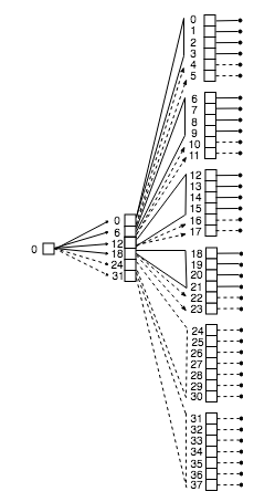
Every time ATA-P is called recursively in a complete parallel level, four processes will call ATA-P on the four sub-matrices of defined in Equation (3), whilst the other two processes will execute HASA-P to compute the two rectangular products that are required to obtain (see equation (2)). In a complete parallel level, HASA-P execution implies that seven processes execute HASA-P, each on its own sub-data. A representation of how processes are distributed in ATA-P is depicted in Figure 1, that shows the tree structure of the processes organization for two complete parallel levels.
The structure described above, according to which ATA-P or HASA-P are called, can be used to derive the function , that we use to calculate the number of processes needed to accomplish complete parallel levels of ATA-P. In particular it holds that:
| (4) | |||
Given the number of available processors , the maximum number of executable complete parallel levels is:
| (5) |
If the number of available processes is equal to , for some , then no more processes are available and therefore all active processes will continue their task sequentially.
The alternative case occurs when . This corresponds to the scenario where no more complete parallel levels can be executed, yet some computational resources are still available. In this case the remaining processes are distributed in order to lighten the workloads of those processes involved in the complete parallel levels. When this event occurs, an incomplete parallel level is set between the -th complete parallel level and the sequential calls.
When an incomplete parallel level can be performed, processes are distributed according to the following idea. To spread the processes as evenly as possible, the value is calculated as follows:
| (6) |
Then, of the still available processes are paired to each process involved in the last complete parallel level. If , there are other processes to distribute. The distribution is realized following a hierarchical chart that exploits a classification of already active processes, based on the heaviness of the task they have to work on. First, we can observe that HASA-P is computationally more expensive than ATA-P, since it involves seven recursive calls instead of six. Hence HASA-P has the highest priority. The second factor used to establish process priority is represented by the size of the sub-problem assigned to a call. In fact, if and are not a power of 2, after a certain number of recursive calls, it holds that and . Therefore, the size of the data of some processes may be higher.
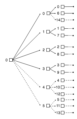
Hence, processes may be ordered depending on the call (HASA-P or ATA-P) first, and on the size of the sub-problem as second parameter. In summary, the last processes are paired, in a orderly way, to: (1) processes that are in charge of HASA-P calls, (2) processes that work on larger sub-problems. An example of how processes are distributed in a incomplete parallel level is depicted in Figure 2, for . In this case, and lefties. The value of resulting from equation (6) is 1, hence each of the processes can be paired to one of the lefties processes. As for the further remaining three processes, two are paired associated to processes performing HASA (namely, one is associated to the process having father with rank 4 and one is associated to the process having father with rank 5), whereas the third process must be associated to one of the process with higher sub-data size, that in this case is only .
4.2 Implementation details
The parallel algorithm has been implemented using MPI for running on a multiprocessor system (see Section 6). Once the MPI environment is initialized, every process gets its own identifying rank through the MPI function MPI_rank. In addition to the input arguments given to Algorithm 1 in the sequential version, a parallel recursive call to ATA-P also reads:
- •
the index of the level it is working on;
- •
the maximum number of complete parallel levels;
- •
father the rank of the father of the process that is serving the current call;
- •
lefties the number of processes beyond the ones needed to accomplish complete parallel levels.
The argument father is the rank of the process that has called ATA-P, tracing the tree of the recursive calls (see Figure 1).
We assume that . When the function is first launched, the identifier of the generated parallel level is 1, and the father is process 0. At each parallel level of ATA-P, the sub-problems are divided among processes depending on their task. Initially, for each parallel recursive call, an array of size 6 called is defined in the following way. In the level , the -th element of is defined as = father + , for , while the 6-th element is defined as = father + , where . Afterwards, recursive calls to complete parallel levels are assigned to processes with rank in [) if , and to process with rank [, ) otherwise, for working on different sub-problems. Notice that process is . Similarly, in each parallel level of HASA-P, the array of size 7 is defined in such a way that the -th element of is = father + , where again . It is easy to understand why the numbering is constructed in this way by looking at the tree shown in Figure 1.
The pseudocode of a simplified version of ATA-P is reported in Algorithm 2. This version of the algorithm is simplified in the sense that we assume that is taken equal to , for some , and this implies that only complete parallel levels are executed. Since the input argument lefties is necessary only when an incomplete parallel level can be performed, it is omitted in Algorithm 2, (in fact, in this case lefties is equal to 0, being ). This simplification can be removed simply by adding the management of the set of lefties processes that we have when and that is described in Section 4.1.
4.3 Communication between processes
In the following sections 4.3.1 and 4.3.2, we shall describe how communication between processes was developed. For both functions ATA-P and HASA-P, we combined communicators and point-to-point communication. Communicators group together processes that may be organized in different topology within the communicator they belong to. Point-to-point communication allows two specific processes to share data.
Input:
Output: Lower triangular part of
4.3.1 Communication in ATA-P
In this section we describe how communication is carried out in ATA-P complete parallel levels. In each complete parallel level, the six processes generated by the call to ATA-P are responsible for the four recursive calls to ATA-P and for the two calls to HASA-P, and are now identified by rank (where is the array defined as in the previous section). Recall that, for each call, is the father of itself and of the remaining elements of . Tasks are divided in the following way:
runs ATA-P on ;
runs ATA-P on ;
runs ATA-P on ;
runs ATA-P on ;
runs HASA-P on (, ;
runs HASA-P on (, .
Each of the three pairs of processes (,), (, ), and (, ) is responsible for computing the two addend of the three sub-matrices of (see equation (2)). Four communicators are created at this stage. Three communicators link together the addends of each of the three sub-matrices , and . To this end, an MPI reduction performing a matrix sum is executed within each of such communicators. As a result, processes , and have , and respectively. The fourth communicator, that we call Current World, collects together all processors in . Current World is used to handle MPI barriers to synchronize processes, guaranteeing safe communication. By convention, the root of communication is the process with the lowest rank in the current communicator. Blocking Send and Receive functions are employed to transfer and from and , respectively, to processor , which is now in charge of defining and returning . Communication is represented thoroughly in Figure 3.

4.3.2 Communication in HASA-P
Here below we show how we implemented the communication system in a HASA-P complete parallel level. In each complete parallel level, the seven processes with rank are responsible for the seven recursive calls to HASA-P.
In particular if HASA is run on matrices and , to obtain their product , the workload is distributed among processes as follows:
runs HASA on (, ;
runs HASA on (, ;
runs HASA on (, ;
runs HASA on (,
runs HASA on (, ;
runs HASA on (, ;
runs HASA on (, .
When processes complete their work, the product matrix is obtained calculating its four blocks as follows:
;
.
Similarly to how was done for ATA-P, four communicators (one for each block of ) are created at this stage. Processes computing a term that appears in more than one block of (namely, all terms but and ) belong to two communicators. A MPI reduction allows to store , in the root of each communicator. Once all MPI reductions are completed, all data is sent to using Send/Receive functions. is responsible for recovering and returning . Similarly to what described for ATA-P, synchronization among processes is achieved by creating a Current World communicator that includes all processes , . Communicators are represented in Figure 4.

5 Communication model and cost
Our communication model is similar to the one used in [2]. We consider latency and bandwidth costs, denoted as and , respectively. Latency cost is the communicated message count while bandwidth cost is expressed in terms of communicated word count. Message and word counts are computed along the critical path introduced in [26]. If is the time spent for communicating a message and is the time for communicating a word, then the total communication cost is given by:
The number of messages that are exchanged between processes depends on how many complete parallel levels of processes can be layered, (see equation (5)). Notice that it holds ; this is because of the number of nodes of the ideal tree that processes are distributed on (see Figure 1 for an example); more precisely, we may observe that for all it holds that .
In a ATA-P communication step, three MPI reductions occurs simultaneously. Afterwards, two messages are sent to the root of the Current World communicator (see Figures 3 B) and C)). In a HASA-P communication step, four MPI reductions are performed at the same time, and three messages are sent to the Current World root. Since HASA-P is recalled on levels, it holds that , that is in general. Hence, we can observe that the achieved latency is lower than the one reached in [2] for generic multiplication, but communication suffers from high bandwidth cost (). Insights on this fact are given in Section 6.3.2.
6 Performance evaluation
In this section we describe the results of experimental tests carried out in order to assess ATA-P. We implemented ATA-P using MPI and tested it on a cluster of Intel processors. Performances are analyzed using different number of processors and several features for parallel algorithms were investigated.
6.1 Experimental setup
Performances have been tested on a small subset of nodes of the Galileo cluster, installed in CINECA (Bologna, Italy), [1]. It is an IBM NeXtScale, Linux Infiniband Cluster consisting of 360 nodes 2 x 18-cores Intel Xeon E5-2697 v4 (Broadwell) processors (2.30 GHz), and 15 nodes 2 x 8-cores Intel Haswell (2.40 Ghz ) processors endowed with 2 nVidia K80 GPUs.
6.2 Experimental results
We studied the performances of ATA-P in terms of execution time, speed-up, efficiency and Karp-Flatt metric. For tests, we considered randomly generated square matrices of size and . Tests have been carried out for the following values of activated processes . The cases correspond to a parallel execution with complete parallel levels, whereas the remaining values of generate incomplete parallel levels.
Execution times for matrix size and are depicted in Figure 5. For , the execution time is obtained running the sequential implementation of ATA. From Figure 5, we can observe that for values of that do not correspond to the activation of complete parallel levels there is a degradation in the trend of the execution time. On the contrary when the number of processes allows to generate complete parallel levels, the execution time improves. This aspect is also observable in Figure 6, where we show the speed-up values. We can observe that for matrices of size the speed-up maximum value is , and is obtained for , see Figure 6. The trend of the execution times shown in Figure 5 is strictly decreasing, highlighting the good scalability of the approach.
The efficiency is computed as the ratio between the speed-up and the number of processes , and ranges from 0.66 (obtained for ) to 0.26 (obtained for ), as reported in Figure 7. As expected, efficiency has a decreasing trend, except for , where it grows. A first observation about this fact is the following: for , exactly 2 complete parallel levels can be performed, while for it holds that and the remaining 12 processes are paired to the processes in order to create an incomplete parallel level. Therefore, some portions of executed code are not shared in the two cases arising from having and . Further comments on this phenomenon are in Section 6.3.2.
Finally, in Figure 8, the Karp-Flatt metric values, giving the experimentally determined serial fraction, are reported. The Karp-Flatt metric was first introduced in [16] and depicts the fraction of time spent by a parallel program to perform serial code, . It is defined as follows:
| (7) |
where is the speed-up and is the number of processes. As we can see in Figure 8, values of are small and decreasing, meaning that there is no significant parallel overhead and that the portion of serial code that is executed is very low.
6.3 Discussion of performance results
The performance assessment parameters show that ATA is scalable and highlight high speed-up and negligible portions of executed serial code. Efficiency has a frequently observed decreasing trend that is due to intrinsic parallel overhead when the number of processes grows. In this section we make two key observations that may be taken into account for improving the performances of ATA-P.
6.3.1 Process redistribution
As we described in Section 4, every time ATA-P and HASA-P are called recursively, in each complete parallel level one process is responsible for one recursive call, either to ATA-P or to HASA-P. Nevertheless, the computational cost of HASA-P is higher than the one of ATA-P. This results in a idle time for those processes performing ATA-P that worsen efficiency. As a matter of fact, the peak of efficiency for (see Figure 7) is rather due to a low efficiency for and , that are the two configurations that report the highest time difference between processes executing ATA-P and those performing HASA-P. A strategy to overcome this issue can be to distribute processes so that more processes are responsible for HASA-P calls, at the expenses of more workload for those performing ATA-P.
6.3.2 Data redistribution
In Section 5 we discussed the expression for latency and bandwidth of ATA-P. We noticed that the number of sent messages is small, but that the maximum size of sent messages is independent from . Because of the low latency, this does not introduce a very appreciable delay when the number of processes is low, but it may introduce non negligible overhead for a very high number of processes. In the configurations that we investigated, the maximum percentage of time spent for communication ranges between 0.14% (, maximum time spent for communication is 0.08s) and 0.46% (, maximum time spent for communication is 0.16s) of the total parallel execution time. A possible solution to high bandwidth is to divide matrix size such that all processes work on the same amount of data and avoiding intermediate communication between processors.
7 Conclusions and future work
We have defined a cache-oblivious recursive algorithm for the matrix multiplication, ATA, that is an operation that has applications in several problems in geometry, linear algebra, statistics, etc. The number of multiplications performed on matrices of size is upper-bounded by , in the face of products for conventional multiplication algorithm; this is achieved because ATA includes recursive calls to generalized Strassen’s algorithm for rectangular matrix multiplications. The algorithm was implemented in parallel using MPI and tested on a cluster. MPI communication facilities were used to perform smart communication in each parallel execution of ATA. Latency is low and the performances were assessed in terms of several performance evaluation indices, highlighting good scalability, low parallel overhead and negligible fraction of inherently sequential code. We detected possible improvements for the enhancement of parallel performances consisting in a different balance for task distribution among processes, and a more equally spread load of data among processors. We plan to find a trade-off between the two proposed improvements. Also, we believe that existing performance evaluation indices penalize the test results of systems where the execution time of employed processors do not overlap perfectly: first and foremost, conventional efficiency does not take into account the amount of time during which not all processors are actively working; yet processes performing faster operations may use idle time for fulfilling additional tasks if the algorithm is integrated in a more complex system. We believe that a more accurate formulation for efficiency and speed-up may be useful to assess more truthfully systems like the one that we introduced.
Acknowledgements
This work has been partially supported by MIUR grant Excellence Departments 2018-2022, assigned to the Computer Science Department of Sapienza University of Rome. The experimental part has been run on the Galileo cluster, located in Cineca, thanks to Class C ISCRA Project n. HP10CCM8RG.
References
- [1] UG3.3: GALILEO UserGuide. https://wiki.u-gov.it/confluence/display/SCAIUS/UG3.3\%3A+GALILEO+UserGuide, 2018. [Online; accessed 11-January-2019].
- [2] G. Ballard, J. Demmel, O. Holtz, B. Lipshitz, and O. Schwartz. Communication-optimal parallel algorithm for Strassen’s matrix multiplication. In Proc. of the 24 Annual Symposium on Parallelism in Algorithms and Architectures, SPAA’12, pages 193–204. ACM, 2012.
- [3] G. Ballard, J. Demmel, O. Holtz, and O. Schwartz. Graph expansion and communication costs of fast matrix multiplication. In Proc. of the 23 Annual Symposium on Parallelism in Algorithms and Architectures, SPAA’11, pages 1–12. ACM, 2011.
- [4] A.R. Benson and G. Ballard. A framework for practical parallel fast matrix multiplication. In Proc. 20th ACM SIGPLAN Symposium on Principles and Practice of Parallel Programming. PPoPP’15, pages 42–53, 2015.
- [5] R.P. Brent. Algorithms for matrix multiplication, 1970.
- [6] R.P. Brent. Error analysis of algorithms for matrix multiplication and triangular decomposition using Winograd’s identity. Numerische Mathematik, 16:145–156, 1970.
- [7] T.H. Cormen, C.E. Leiserson, R.L. Rivest, and C. Stein. Introduction to Algorithms, Third Ed. MIT Press, 2009.
- [8] P. D’Alberto and A. Nicolau. Adaptive strassen’s matrix multiplication. In Proc. 21st Int. Conf. on Supercomputing, pages 284–292. ACM, 2007.
- [9] F. Desprez and F. Suter. Impact of mixed-parallelism on parallel implementations of the Strassen and Winograd matrix multiplication algorithms. Concurr. Comput.: Pract. Exper., 16(8):771–797, 2004.
- [10] C.C. Douglas, M. Heroux, Gordon G. Slishman, and R.M. Smith. Gemmmw: A portable level 3 BLAS Winograd variant of Strassen’s matrix-matrix multiply algorithm. Journal of Computational Physics, 110(1):1–10, 1994.
- [11] F. Le Gall. Powers of tensors and fast matrix multiplication. In Proc. 39th Int. Symposium on Symbolic and Algebraic Computation, page 296–303, 2014.
- [12] B. Grayson, A. Shah, and R. van de Geijn. A high performance parallel Strassen implementation. Parallel Processing Letters, 6:3–12, 1995.
- [13] N.J. Higham. Exploiting fast matrix multiplication within the level 3 BLAS. ACM Trans. Math. Softw., 16(4):352–368, 1990.
- [14] S. Hunold, T. Rauber, and G. Runger. Combining building blocks for parallel multi–level matrix multiplication. Parallel Computing, 34:411–426, 2008.
- [15] S. Huss-Lederman, E.M. Jacobson, A. Tsao, T. Turnbull, and J.R. Johnson. Implementation of Strassen’s algorithm for matrix multiplication. In Proc. ACM/IEEE Conf. on Supercomputing, 1996.
- [16] A.H. Karp and H.P. Flatt. Measuring parallel processor performance. Communications of the ACM, 33(5):539–543, 1990.
- [17] B. Kumar, C.-H. Huang, R. Johnson, and P. Sadayappan. A tensor product formulation of Strassen’s matrix multiplication algorithm with memory reduction. In Proc. Seventh International Parallel Processing Symposium, pages 582–588, 1993.
- [18] P. Kumar. Cache oblivious algorithms. In Algorithms for Memory Hierarchies, pages 193–212. Springer, 2003.
- [19] Q. Luo and J. Drake. A scalable parallel Strassen’s matrix multiplication algorithm for distributed-memory computers. In Proc. ACM Symposium on Applied Computing, SAC’95, pages 221–226, 1995.
- [20] F. Nielsen. Introduction to MPI: The Message Passing Interface. In Introduction to HPC with MPI for Data Science, pages 21–62. Springer, 2016.
- [21] F. Song, J. Dongarra, and S. Moore. Experiments with Strassen’s algorithm: From sequential to parallel. In Proc. Parallel and Distributed Computing and Systems, (PDCS), 2006.
- [22] A.J. Stothers. On the complexity of matrix multiplication. Journal of Complexity, 19:43–60, 2003.
- [23] G. Strang. Linear Algebra and Its Applications, Fourth Ed. Thomson Brooks/Cole, 2006.
- [24] V. Strassen. Gaussian elimination is not optimal. Numerische mathematik, 13(4):354–356, 1969.
- [25] V.V. Williams. Multiplying matrices faster than Coppersmith-Winograd. In Proc. Forty-fourth Annual ACM Symposium on Theory of Computing, page 887–898, 2012.
- [26] C-Q Yang and Barton P Miller. Critical path analysis for the execution of parallel and distributed programs. In The 8th Int. Conf. on Distributed Computing Systems, pages 366–373. IEEE, 1988.