Simultaneous Sensing Error Recovery and Tomographic Inversion Using an Optimization-based Approach
Abstract
Tomography can be used to reveal internal properties of a 3D object using any penetrating wave. Advanced tomographic imaging techniques, however, are vulnerable to both systematic and random errors associated with the experimental conditions, which are often beyond the capabilities of the state-of-the-art reconstruction techniques such as regularizations. Because they can lead to reduced spatial resolution and even misinterpretation of the underlying sample structures, these errors present a fundamental obstacle to full realization of the capabilities of next-generation physical imaging. In this work, we develop efficient and explicit recovery schemes of the most common experimental error: movement of the center of rotation during the experiment. We formulate new physical models to capture the experimental setup, and we devise new mathematical optimization formulations for reliable inversion of complex samples. We demonstrate and validate the efficacy of our approach on synthetic data under known perturbations of the center of rotation.
keywords
Tomographic reconstruction, Sensing error, Self-calibration, Nonlinear optimizationAMS
68Q25, 68R10, 68U051 Introduction
Tomographic imaging has had a revolutionary impact on medicine, physics, and chemistry. Even so, the problem of reconstructing an image from tomographic data remains challenging in many interesting cases, such as when the amount of available data is limited and/or the problem is ill posed (in the sense that canonical metrics used to assess the discrepancy between a reconstruction and the measured data generally possess many local minima). This ill posedness makes reconstructions susceptible to experimental errors, in particular, to errors stemming from mismatches between the experimental configuration and the assumptions of the measurement process. Recovering such errors is crucial for realizing the gains from improvements in measurement and experimental hardware, such as the improved resolution promised by brighter, more coherent next-generation light sources. Sample drift [28] and beam drift [36] are two fundamental sources of error. These errors can often arise from the drift of the center of rotation (CoR) of the imaging stage during data acquisition [2], which is the focus of this work.
In computerized tomography, the object or sample being imaged is placed on a stage and irradiated with parallel beams of x-rays. As the rays pass through the object, they are partially absorbed according to the object’s composition. Radiation that passes through the object unabsorbed is collected by a detector, producing an x-ray “shadow” or “projection” of the object. By rotating the object and repeating the process, one obtains projections of the object as illuminated from several different directions. One then uses these projections to reconstruct an image of the object and its interior [22].
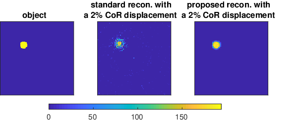
Imperfections in the experimental apparatus can cause the CoR of the imaging stage to vary slightly over the course of this process. When this happens, the projections from different angles will not be properly aligned relative to one another, and failing to account for this misalignment during reconstruction may result in a smeared image (loss of resolution) or, worse, an image that is completely incorrect. Moreover, even a small error in the CoR can yield a large error in the reconstruction, as is illustrated by the experiment of Fig. 1. The image on the left shows the object—a small, solid circle—and the image in the middle shows the result of a standard tomographic reconstruction without addressing the CoR shift from a sequence of measurements in which the CoR is perturbed by a 2% displacement relative to the size of the object domain. The reconstructed image obtained by not correcting for this perturbation looks very different from the true object. We also demonstrate the reconstruction of the approach we propose in this paper on the right side, which almost perfectly resembles the true object.
In the past, it has been possible largely to ignore errors like these, as the drifts have been small compared with the widths of the beams used to illuminate the object. With demand for increasingly finer resolutions leading from higher-quality light sources with narrower beams, however, these errors can no longer be ignored. Potential approaches to this problem include the incorporation of prior knowledge into the reconstruction process using Bayesian frameworks [17, 33, 34] and the use of regularizers to promote sparsity or smoothness of the reconstruction [14, 10, 23, 30, 20]. One can also collect additional data (beyond x-ray projections) that is less sensitive to experimental errors and use this data to help with the reconstruction [7]. Unfortunately, the improvement in tomographic hardware has been so great that these generic approaches, which apply more widely to problems other than CoR drift recovery, are not likely to be sufficient. In the case of CoR drift, we show (in Sec. 5) that standard regularization approaches fail even when the regularization parameter value is chosen in an ideal way.
Much research effort has been devoted to tackling the CoR recovery problem. For example, a typical approach to recovering a single, unknown CoR is to use a pair of projections that are reflections of one another to estimate a detector offset that can be used to shift the projections into the correct positions [40, 27]. This approach is highly sensitive to the accuracy of the mirrored alignment, and its use of such a small number of projections to perform the correction makes it susceptible to noise and other effects of limited data, potentially resulting in a low-contrast recovery. Moreover, mirrored pairs of projections are not always available in practice. Azvedo et al. [2] proposed a method to estimate the CoR based on the preservation of photon counts passing across the sample, which requires almost perfect measurement. The most common technique is to compute cross correlations between projections acquired from successive rotations [11, 1, 18]; however, this approach is limited to simple and relatively homogeneous samples, since there is no good way to rank one feature as “more important” than another when two projections contain very distinguishable features. A similar approach involves manual alignment of the projections using a known “hotspot” in the object as a reference. This process can be labor-intensive and cannot be used if a hotspot cannot be identified. Recently, a new technique known as iterative reprojection has been introduced in which one recovers projection alignments and reconstructs the image simultaneously using an iterative procedure [35, 19, 39, 13]. The basic idea is to alternate between a few iterations of projection alignment and a few iterations of reconstruction until a “forward model” of the experimental setup and an “inverse model” of the reconstruction process are consistent with one another. This approach can yield better accuracy, especially for noisy, limited data.
One deficiency of the iterative reprojection methods that have emerged thus far is that the update of the projection alignment and the update of the reconstruction are not fully coupled. As a result, some mismatch remains between the alignment of the projections and the experimental configuration assumed by the reconstruction process. In this work, we propose to address this problem using a novel joint inversion framework based on optimization in which we explicitly model and recover for CoR drift. Our proposed model is flexible, making no assumptions about when and where the drift happens. Our new approach is easier to automate than existing approaches and can be more robust in the context of poor data quality and limited prior knowledge of the object being imaged.
In Sec. 2, we describe our mathematical forward models of the CoR drift error in the experiment and show how to embed these models into the reconstruction scheme. In Sec. 3, we describe our simultaneous reconstruction approach for recovering the object and the experimental error, including the formulation of the objective function. In Sec. 4, we describe the algorithm for solving the resulting optimization problem and its complexity. In Sec. 5, we present some numerical illustrations comparing the performance of our simultaneous inversion method with that of existing approaches using a few synthetic examples. In Sec. 6, we summarize the proposed method and discuss a few directions for future research.
For simplicity, we confine ourselves to reconstructing 2D images, although our methods work just as well in 3D.
2 Mathematical Model
In this section, we describe our model for the tomographic imaging process. For further details on tomography, we refer the reader to [21].
2.1 Radon Transform
The fundamental mathematical tool in tomography is the Radon transform [32], defined for a compactly supported function by
| (2.1) |
where is the Dirac delta function. Throughout this article, we consider the restricted domain given by and , and we assume, as will always be the case in practice, that is well-enough behaved that the integral makes sense. The Radon transform of a function is frequently called its sinogram.
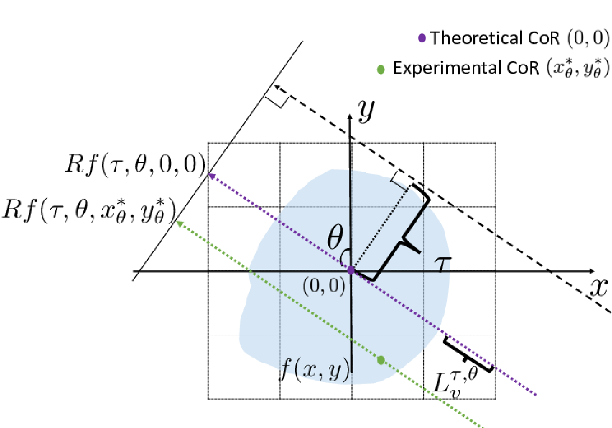
The projections that are measured in the tomographic x-ray imaging process are values of the Radon transform of the object’s attenuation coefficient , a function that describes the propensity of the object to absorb x-rays at each point in the object’s support. The angle encodes the direction from which the beams approach the object; and given that direction, encodes the position of the beam. If the CoR shifts from the origin to , as the imaging stage rotates through the angle , the projections we measure come not from (2.1) but from the CoR-shifted Radon transform
| (2.2) |
For a derivation of this equation, see Appendix B. As illustrated in Fig. 2, is the integral of along the purple line perpendicular to the direction determined by the angle and at a distance from the origin. Alternatively, the purple line is obtained by rotating from its previous position, which overlays with the -axis, degrees with respect to CoR . However, if the CoR is shifted from , denoted by the purple dot, to the green dot, we obtain a different projection as .
To recover for the difference in CoR, we need a way to convert (2.2) back into (2.1). This is easy: we have
| (2.3) |
where
| (2.4) |
The simple relationship (2.3)–(2.4) forms the basis for our algorithm. We rotate the imaging stage through an angle with the intent of measuring , but we instead measure due to drift of the CoR. The identity (2.3) shows that all we need to do is translate (in ) the Radon transform that we measured by an amount , which is related to the true CoR by (2.4). As we later show, given sufficient data, we can estimate the drift-induced using an optimization procedure.
2.2 Discrete Tomography
In practice, we cannot recover the desired object property (e.g., attenuation coefficient) at all points in space. Instead, we discretize the space (containing the compact object) being imaged into pixels and vectorize it to an array . Let be the value of the object property we intend to recover on the pixel , and let denote the discretized image. Given parameters and , we calculate a discrete Radon transform of via
where is the length of the intersection of the beam described by and with the pixel , see Fig. 2. It is this relationship that we must invert to reconstruct our image: knowing , we wish to find for each pixel .
In addition to needing to consider the image discretely, we must also “discretize the beams”: we have access only to for a limited number of values of and . The values of we use are fixed and equally spaced and are identical for each . We denote the collection of values of (sometimes called “beamlets”) by and the collection of values of by ; accordingly, is the number of beamlets, and is the number of angles. In reality, the resolution of is decided by the energy level of the radiation source and by the detector resolution [3].
Thus, for each angle , our measurement apparatus ideally produces a set of samples of , equally spaced in , which we take as values of . Because of the drift in the CoR, however, our samples are actually from instead. We can account for this drift by recomputing the to be consistent with the change in CoR, but we wish to avoid doing so because calculating these values (potentially many times) is expensive. Instead, we calculate them once, assuming that the CoR is at the origin, and recover for the change in CoR by translating the projections.
2.3 Aligning the Projections
In principle, translating in the variable by is an easy task—the answer is just —but since we have access only to samples of at , we cannot do this. Since the samples come from equally spaced points, a natural idea is to effect the translation by using the discrete Fourier transform, which is mathematically equivalent to forming a trigonometric interpolant to through the points and translating the interpolant. This approach works, but the images recovered in this way in practice are contaminated with ringing artifacts [4, pp. 209]. To fix this problem, we apply a low-pass filter—a normalized Gaussian filter with standard deviation —to damp the high-order Fourier coefficients.
An alternative way to understand the translation process is as follows. Translating , viewed as a function of only, by is equivalent to convolving with a Dirac delta function centered at : , where . We regularize by replacing it with a Gaussian,
| (2.5) |
and instead compute the convolution , which we do by sampling and on the same equally spaced grid and using the discrete Fourier transform.
How should one choose the hyperparameter ? Let be our approximation to 11 1 As in the preceding paragraph, the in in this definition is understood to be the CoR-shifted Radon transform. Our notation emphasizes our hope that . obtained from the discrete Fourier transform. By the error analysis presented in Appendix C, if the (attenuation coefficient of the) object being imaged is twice continuously differentiable, then
| (2.6) |
The second term on the right-hand side of (2.6) represents the error incurred in our Gaussian regularization of the delta function, while the third term represents the discretization error due to the limited number of measurements. A trade-off between the two exists: a narrower Gaussian (smaller ) implies a more faithful translation, but it requires more measurements (greater ) to approximate accurately.
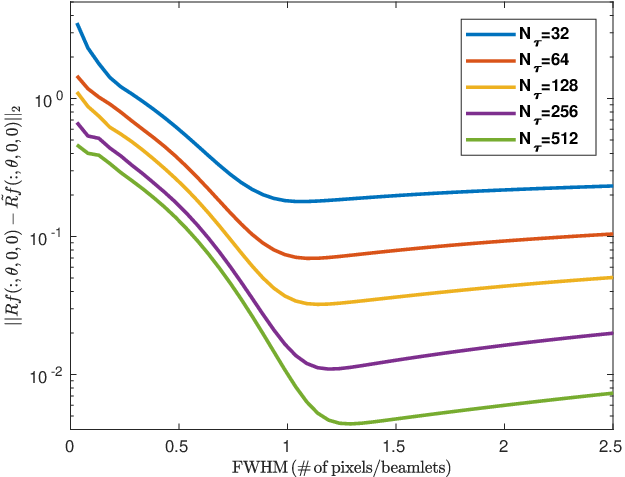
We choose to have the full width at half maximum (FWHM) of the Gaussian regularizer to cover one unit of beamlet width. Since the FWHM for a Gaussian with variance is given by , this means that we choose . Observe that this choice is supported by Fig. 3, which displays the approximation error in Eqn. (2.6) in the simulated beam data from Fig. 4. For the values of considered, the choice is roughly the point at which the second error term in (2.6) takes over from the first.
2.4 Numerical Illustration


To illustrate the effects of the approximation (2.6) in the context of a complete image, we perform a simulation using a standard MRI test image. We simulate beam data from a variety of angles, assuming that as the object rotates, it does so about a CoR where and represent two different angles; in other words, there is only one CoR drift in the beginning of the experiment. The results are displayed in Fig. 4a, where , , and equally spaced in . The leftmost panel shows the test image; the red dot marks the CoR . The second panel shows the sinogram obtained from this data. The third panel shows the sinogram that we would have obtained in the absence of the drift in CoR. The fourth panel shows the sinogram that we obtain after performing the recovering translations using the approach outlined in the preceding subsection. The drift-free and drift-recovered sinograms are in excellent agreement, even in the presence of the errors described by (2.6).
In Fig. 4b, we repeat the experiment of Fig. 4a except that the CoR changes each time the object is rotated instead of just once at the beginning of the experiment; in other words, . The trail of red dots in the leftmost panel shows how the CoR drifts across the image as the data is acquired. The drift-free and drift-recovered sinograms are again in excellent agreement. From a practical perspective, the additional “jitter” due to the multiple shifts of CoR—readily apparent in the measured sinogram—complicates the alignment process significantly. Nevertheless, the algorithm we propose next is able to handle multiple shifts.
3 Optimization-Based Reconstruction Algorithm
In the experiments of Sec. 2.4, we assumed exact knowledge of the CoR and the corresponding translation parameter . In practice, we must estimate these parameters from the data. As described in Sec. 1, the best techniques used to date generally do this iteratively by alternating between using the current parameters to reconstruct the image and using the reconstruction to update the parameters. Instead, we propose to estimate the parameters and reconstruct the image concurrently.
The most straightforward approach would be to try to estimate and and obtain from these estimates using (2.4); we refer to this as the explicit approach, since we try to find the CoR explicitly. Alternatively, we can skip the estimation of and and try to solve for directly; we call this the implicit approach. One major difference between the explicit and implicit approaches is the different dimension of unknown variables. In general, each corresponds to a pair of , which results in number of CoRs to be recovered. If one knows which angles have the CoR drifts, however, the number of pairs can be reduced to the exact number of drifts.
To exploit the correlations between and , we formulate the reconstruction problem as simultaneously recovering the CoR and recovering the object. Therefore, the final explicit reconstruction problem is
| (3.7) |
where , , is due to the physical nature of mass, is the measurement data, is the translated sinogram by (2.4), and is determined based on the standard 2D Radon mapping with an implied CoR of .
As a side note, tomographic reconstruction without CoR error recovery is typically formulated as
| (3.8) |
which is equivalent to Eq. (3.7) for
The first-order derivative of the objective function (3.7) is
| (3.9) |
In (3.9), and are
and
respectively, where is the Hadamard product, and is the row of . A major difference compared with the single CoR-shift case is the increased computational cost. Instead of having only two extra parameters, this case has extra parameters.
For now, we have been focusing on explicitly recovering the coordinates of the CoRs . Alternatively, we can reformulate the optimization problem as finding the optimal shifts for each angle, which results in the implicit problem
| (3.10) |
where and . The derivative of the objective function in (3.10) is similar to (3.9) but simpler, so we will not describe it here. In the case of multiple CoR shifts, the advantage of this formulation is the reduced number of extra parameters by a factor of 2. Notice that given a fixed CoR, the Radon transform has the property that different transformations (e.g., translation or rotation) of an object will result in different sinograms; see Appendix A. These properties suggest that any pair of transformed object and its corresponding sinogram is an optimal solution of the reconstruction. Therefore, the proposed optimization problem, either explicit or implicit, will not have a unique solution. In other words, if two objects are related by equal (up to translations and rotations), then the two objects, together with their corresponding sinograms, are equivalent from the perspective of the optimization problems in (3.7) and (3.10).
4 Optimization Complexity and Computational Expense
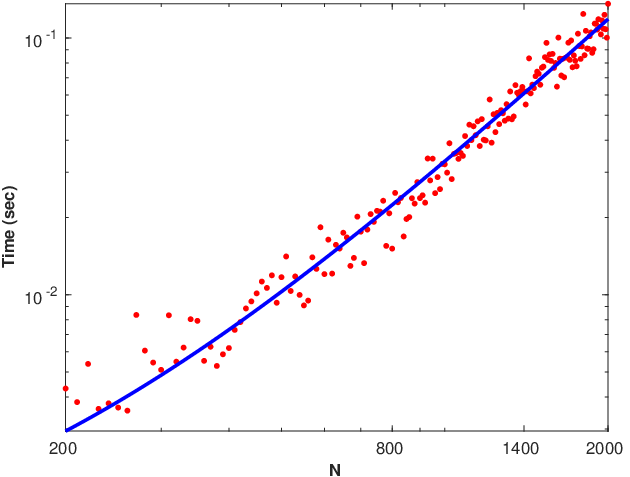
Since the complexity of Eq. (2.4) is negligible, we analyze only the computational complexity of the implicit approach (3.10). The calculation of Eq. (3.10) requires about flops given the relationship , and it includes 1 misfit calculation and 3 FFTs required in operator . Figure 5 shows a log-log plot of the computational time of one (function, gradient) evaluation for increased number of , given . With a model fit to the time result, the time complexity is on the order of which is consistent with our analytical approximation considering in general.
The optimization solver we use in the numerical experiments is an inexact truncated-Newton (TN) method [29] with a preconditioned conjugate gradient (PPCG) [31, pp. 460] subproblem solver to compute the search direction. The result, summarized in Alg. 1, is a large-scale optimization solver with memory efficiency well suited for the high computational complexity required by the resulting nonlinear, nonconvex optimization problem.
In our implementation, we do not form the Hessian ; instead, we approximate the Hessian-vector product required in PPCG by taking finite differences with values. An estimation of the complexity of TN is provided as follows. Each outer iteration needs the following computations with respect to the number of unknown parameters:
- •
1 infinity-norm calculation, 1 vector addition, and 2 (function, gradient) evaluations
- •
a number of PPCG iterations, with cost per inner iteration given by
- –
1 (function, gradient) evaluation,
- –
4 inner products, and
- –
5 “vector+constantvector” operations
- –
In our experience, on average, 5 PPCG iterations are required per outer TN iteration. The overall cost of one TN iteration for solving (3.10) amounts to floating-point operations, plus 7 (function, gradient) evaluations, whose complexity is .
5 Numerical Results
In this section, we examine the performance of the algorithm for both the explicit and implicit cases. The primary goal of our tests is to measure the performance of how well we recover the CoR shift with respect to different initializations, different objects, and different levels of noise in the data. All numerical experiments are performed on a platform with 32 GB of RAM and two Intel E5430 Xeon CPUs. Throughout all the numerical tests, we fix the experimental setup for all the tests as , , and ; that is, the object size is pixels, and the tomographic data is measured by collecting 30 projections over a full rotation of radians. We also choose the stopping criteria of TN to be .
As indicated in Sec. 3, our proposed optimization problem does not have a unique solution in the sense that the reconstructed object can be a translated or rotated version of the ground truth. Therefore, the error metric we use to measure the reconstruction quality cannot be simply the mean squared error. To resemble the human visual system, we utilize the structural similarity (SSIM) metric from [37] to quantify the reconstruction quality. Given two images and of the same dimension, the SSIM index is a measure of the similarity between and and is defined by
where and are small, positive constants; and are the mean and variance, respectively, of ; and are the mean and variance, respectively, of ; and is the covariance of and . Notice that for nonnegative and , . The closer the value of is to , the greater is the similarity between and .
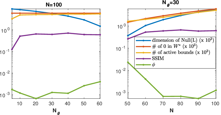
We emphasize that in this work our focus is on the development of a joint framework to account for general CoR shifts. To isolate the contributions of our proposed approach to the reconstruction performance, we do not consider any additional regularization technique in this work. Additionally, the nonnegative constraint on serves as a soft regularizer, which means we do not need to add a regularizer and can instead show the benefit of our approach by itself [8, 5]. As suggested by Fig. 6, where we test the performance of TN on various settings for the traditional tomography problem (3.8), we observe that as long as the dimension of Null() is close to the number of zeros of the object, the reconstruction quality is stable and satisfactory based on SSIM and the objective value of problem (3.8). Since the object domain always has a zero support to account for the field of view during the rotation, the dimension of Null() typically is proportional to the number of zeros in , and this explains the satisfactory reconstruction result from seemingly underdetermined system.
5.1 Analysis of Initialization
In this section, we test the sensitivity of the proposed algorithm to the initialization of .
We first consider the case of a single CoR shift that happens at the beginning of the experiment on a standard Shepp-Logan phantom object. The CoR is denoted by the red dot on top of the ground truth in Fig. 7 (far left). The upper left panel of Fig. 7 shows the standard reconstruction without considering the shift of the CoR, and we observe that it is far from the ground truth. We also include reconstructions obtained by adding standard regularizers. In particular, we consider - and -regularizers [25, 15] on the variable , respectively given by
| (5.11) |
and
| (5.12) |
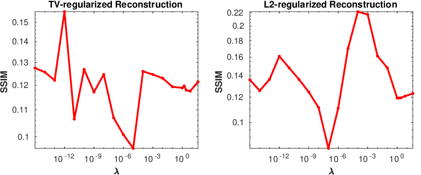
where is the Laplacian operator, denotes the spatial gradient, and is the regularizer parameter that balances the misfit term and regularization term. One approach to choose would be the L-curve method [16]. Instead, however, we choose to be the value that gives the best reconstruction as measured by the SSIM index (see Fig. 8). This is an idealistic choice of that is impractical. The results given in the upper middle and upper right panels demonstrate this assertion and show that standard regularization techniques are not able to improve the reconstruction quality in the presence of even a single CoR shift. Since even an optimal performs poorly for CoR recovery, for the rest of our experiments we do not report results from regularization techniques.
We also compare our reconstruction result with the most popular approach for the case of a single CoR drift [27]. The basic idea is to utilize the fact that when the CoR is the origin, the projection at angle should be a reflection of the projection at angle . Therefore, the CoR shift can be estimated by aligning these two projections. In our case, as is often the case in practice, exactly reflecting directions are not available; instead, we choose the pair of angles and from the available 30 projections. We align these two projections by cross-correlation [40] and use the estimated CoR shift to translate the collected sinogram. The reconstruction from the shifted sinogram is reported in the lower left panel. We also report the reconstruction using the true CoR in the lower right panel. The lower middle panel shows the reconstruction obtained by the proposed explicit approach, which clearly resembles the ground truth the best.

The next test is to optimize the explicit problem (3.7) and the implicit problem (3.10) in order to recover and , respectively. Given an initial as the center, left top corner (NW), left bottom corner (SW), right top corner (NE), and right bottom corner (SE) of the object domain, respectively, and initialization , the performance is shown in Fig. 9. In this test, the explicit approach consistently recovers objects that are better compared with the implicit approach, which struggles for certain initializations. This observation is also reflected in the objective value and the reconstruction quality. In addition, the explicit approach takes fewer iterations to converge to smaller objective values compared with the implicit approach. The explicit approach also provides relatively better reconstruction quality as measured by SSIM index.

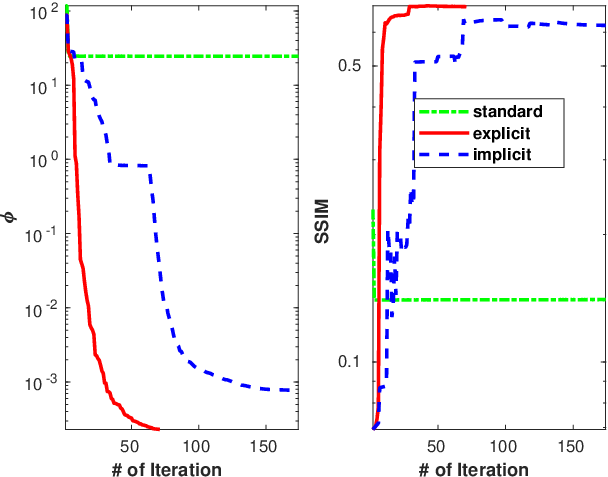
In Fig. 10, we also show the iterative progress of the optimization problems (3.8), (3.7), and (3.10) respectively for the single CoR-shift case. The left graph shows the progress of the objective value for the three approaches. Standard tomographic reconstruction, which refers to reconstruction without error recovery, converges much more slowly than the other two with a much higher objective value, while the explicit approach reduces the objective value even further than the implicit approach because of the reduced number of variables. The right graph compares the progress of the SSIM index for the three approaches, which is somewhat consistent with the function value reduction. We observe that the explicit approach provides the best reconstruction quality in terms of SSIM compared with the other two approaches, while the standard approach performs the worst because it does not attempt to recover for the error in CoR.

The next test concerns solving the reconstruction problem with multiple CoR shifts in the sense that every rotation has its own CoR. This problem setting is illustrated in Fig. 12, where the ground truth is again the Shepp-Logan phantom and the trajectory of the dynamic CoR is denoted by connected red dots. The second panel shows the reconstruction without CoR recovery, and the third panel shows the reconstruction with error recovery. Again, we tested the performance of the explicit and the implicit algorithm; the results are shown in Fig. 13. This time we observe that the reconstruction quality of the implicit approach is comparable to the explicit approach but is more sensitive to the initialization. In the multiple CoR-shifts case, however, the convergence of the implicit approach is faster because of its reduced number of variables compared with explicit approach. Again, the performance difference between the explicit and implicit approaches is reflected in the objective value and the corresponding SSIM index. More importantly, as shown in Fig. 11, both approaches are able to remove the jitters introduced by multiple CoR shifts and return a clean sinogram. The consistency between the objective value and SSIM index suggests that, in the case of limited knowledge about the object, the objective value can be reliable to judge the reconstruction quality of different local minima.
We note that as long as the shift parameters are initialized to zero, the performance is relatively stable and less susceptible to the initialization of the object. The reason is that choosing the initial shift as zeros is equivalent to providing the initialization of the object as the reconstruction without error recovery, which is closer to the true solution than the reconstruction from a randomly perturbed sinogram. Therefore, choosing zeros for the initial shifting parameters performs better, and this initialization will be our choice for the rest of the tests.


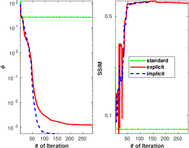
Similar to the single CoR case, we compare the iterative progress provided by the standard reconstruction, the explicit approach, and the implicit approach for the multiple CoR-shifts case; the results are shown in Fig. 14. As expected, the standard approach converges rapidly to a local minimum that has a high objective value. More importantly, the implicit approach provides a better objective value than does the explicit approach. The reconstruction quality (right panel of Fig. 14) shows comparable performance between the explicit and the implicit approaches.
5.2 Noisy Data
In practice, the experimental data is known to be corrupted by noise. In this section, we test the performance of our proposed approach for contaminated data with respect to different levels of (mean zero) Gaussian noise. We start the test for the single CoR shift case as shown in Fig. 15, where the ground truth in this case is the standard MRI image. Similarly, the second and the third panels show the reconstructions without and with error recovery, respectively.
In this case, we compare the performance of the explicit and implicit approaches with the state-of-the-art alignment approach [13] provided by TomoPy 1.1.3 [12], a widely used tomographic data processing and image reconstruction library. The algorithm proposed in [13] is an iterative method that alternates between the alignment of the sinogram and the reconstruction of the object. The alignment step minimizes the misfit between the current sinogram and the newly simulated sinogram based on the current reconstruction. In Fig. 16, we illustrate the reconstruction results returned by the three methods as we increase the noise level in the experimental data; the columns represent an increase in the noise level from 4% to 22%. We observe that the explicit and implicit approaches are comparable with each other. However, the SSIM index for both approaches suggests that the implicit approach provides better reconstruction quality. This observation can be explained by the fact that although the explicit approach can provide a higher contrast image, its ability to remove noise outside of the sample region is not as good as that of the implicit approach. Overall, the performance of our proposed approaches outperforms the alternating algorithm [13] provided by TomoPy.
The last study is to test the performance of our proposed approach for recovering the multiple CoR shifts, as illustrated in Fig. 17. As measured by SSIM, the implicit approach clearly outperforms the other two approaches while the reconstructions of the alternating alignment do not approach the ground truth at all. In Fig. 18, we illustrate the reconstruction results returned by the three methods respectively as we increase the noise level in the same way as the single CoR shift case illustrated earlier. Again, the explicit and implicit approaches are able to provide a reasonable reconstruction, and the implicit approach in this case is able to provide a better reconstruction for the noisier case. Similarly to the single CoR shift case, the performance of our proposed approaches outperforms that of the alternating algorithm dramatically. Therefore, in the case of limited knowledge of the CoR shifts with noisy measurement data, the implicit approach works the best.


6 Conclusions
In this work, we propose a simultaneous inversion framework to address a common yet challenging experimental error in tomographic reconstruction, namely, a shift of the center of rotation. We also derive an analytical model to describe the general center-of-rotation shifts and how the sinograms with and without such shifts relate to each other. We derive an analytical model for the reconstruction framework to recover the center-of-rotation shifts together with the reconstruction of the object. The resulting optimization framework can be tuned to explicitly or implicitly reveal the true CoR locations. It is solved by a derivative-based optimization solver such as a truncated Newton algorithm.
Our numerical results show that when limited and noisy experimental data is available, significant improvements of the reconstruction quality can be achieved by performing the proposed simultaneous inversion. We compare our new approach with a state-of-the-art error reconstruction technique implemented in TomoPy and standard reconstruction techniques with a regularizer approach. For both comparisons, we observe superior results obtained by our approach. Given prior knowledge of how center-of-rotation shifts happen, explicit and implicit approaches can be chosen to maximize the performance, based on their different computational complexities. In particular, the implicit approach shows a stronger capability in more general scenarios such as noisy data.
Discussion: The simultaneous inversion we propose in this work is flexible and does not require extensive knowledge about the experimental system or the object. Even for the single CoR shift, the proposed approach does not require that the sample be completely contained in the field of view or that no nonlinear effects such as diffraction or refraction occur. It can be naturally extended to partially address more complicated experimental error such as per-scan drift. In parallel-beam tomography, the trajectories of the penetrating x-rays result in tomographic projections that form a stack of parallel 2D slices. Traditionally, 3D objects are recovered by reconstructing each slice independently [38]. Therefore, the extension of the proposed approach to a full 3D reconstruction is trivial in parallel-beam tomography. Alternatively, since each 2D slice shares the same CoR, the proposed approach can also be extended to a direct 3D reconstruction without adding an extra degree of freedom. One aspect we can further explore is to incorporate prior knowledge about the experimental system, such as the continuous dynamic of the center-of-rotation movement, into the joint framework as a regularizer on the error parameters. Overall, the challenge we are facing is the increased computational complexity. One way to mitigate this difficulty is to consider a parallel implementation that could be invoked inside a truncated-Newton solver or at the level of processing blocks of experimental data (e.g., per angle). A multigrid approach [24] could also benefit the computational performance.
Acknowledgments
We are grateful to Stefan Vogt, Si Chen, Doga Gursoy, and Francesco De Carlo for introducing us to this problem and for valuable discussions in the preparation of this paper. This material was based upon work supported by the U.S. Department of Energy, Office of Science, under contract DE-AC02-06CH11357.
Appendix A Properties of Radon Transform
We briefly describe a few properties of the Radon transform that explain the equivalence of reconstruction via translation and rotation.
Symmetry: .
Translation: Let . Then
where .
Rotation:
Let where is the polar coordinates of . Then,
Appendix B Derivation of the CoR-Shifted Radon Transform
Here, we present a brief derivation of (2.2). Assume, without loss of generality, that the beam apparatus is initially positioned to measure the Radon transform along the direction corresponding to . By Fig. 2, this amounts to integrating the function representing our object along the vertical lines , . To measure along the direction corresponding to a general angle , we rotate the beam apparatus counterclockwise by .22 2 As described earlier, in the actual experimental setup we rotate the object, not the beam; from a mathematical point of view, it does not matter which we rotate. If the center of rotation is , the line (beam) rotates to the line
By definition, is the integral of along . An easy calculation shows that, ignoring sign, this line is a distance
from the origin. From the geometry of the rotation process we see that the line perpendicular to is inclined at an angle above the (positive) horizontal axis. Hence,
from which (2.2) follows immediately upon substituting in for .
Appendix C Error Analysis for the Projection Alignment Process
In this section, we consider the error in the approximation described in Sec. 2.3. Recall that incorporates both the Gaussian regularization of the Dirac delta and the discretization of the convolution integral using the discrete Fourier transform.
Moving to a more abstract setting, the question is fundamentally one of assessing the error in the approximation , where is some compactly supported function on and where we evaluate the right-hand side by discretizing the convolution integral in a particular way. We lose no generality in assuming that , so we can actually analyze , where we use the shorthand . Since we wish to measure the error with respect to the uniform norm, we need only to consider the error at a single point . We lose no generality in assuming that point is , so we are led to the problem of understanding the error in
| (C.13) |
again, under a specific discretization of the integral on the right-hand side, which in particular includes truncating the domain of the Gaussian .
Thus, we assume that for some , and we define
which is with its support truncated to . Our goal is to understand the error in the approximation to obtained by using the -point (composite) trapezoid rule to discretize the integral in (C.13) on the interval , where :
where is odd33 3 We make this choice solely for notational convenience. Everything we do applies for even as well. and , . (This is mathematically equivalent to evaluating the convolution at one of the points using the discrete Fourier transform.) In particular, we want to know how depends on and .
comprises three sources of error. The first is the regularization error that we incur because :
The second is the truncation error that comes from our limiting the support of the Gaussian:
The third is the discretization error due to our quadrature rule:
We have
| (C.14) |
We will bound by bounding each of the terms on the right-hand side of (C.14) in turn.
Assume that is twice continuously differentiable. Then, Taylor’s theorem (with Lagrange’s form of the remainder) enables us to write
for , where is some function that satisfies for and for . From symmetry of , it thus follows that
and hence we have
| (C.15) |
for the regularization error.
The truncation error is even easier to handle. We have
and so
| (C.16) |
by one of the many available bounds for the complementary error function [6].
The discretization error is trickier. Because is discontinuous on , we cannot apply most standard results, since these results assume continuity of the integrand. Instead, we appeal to the following result from [9], which bounds the error in the trapezoid rule approximation to the integral of a function of bounded variation.
Proposition 1 ([9, Theorem 2.1]).
If is of bounded variation, then
where is the total variation of over .
This result immediately yields a bound of on the error in the composite trapezoid rule, where is the spacing between the grid points.
Because is twice continuously differentiable, it is of bounded variation, and so is . Hence, their product is of bounded variation as well. Moreover, we have
(The norms and total variations are taken over .) Since
and
it follows that
The grid spacing in our trapezoid rule approximation is . It follows that
| (C.17) |
References
- [1] Fernando Amat, Daniel Castaño-Diez, Albert Lawrence, Farshid Moussavi, Hanspeter Winkler, and Mark Horowitz, Alignment of cryo-electron tomography datasets, in Methods in Enzymology, vol. 482, Elsevier, 2010, pp. 343–367.
- [2] Stephen G Azevedo, Daniel J Schneberk, J Patrick Fitch, and Harry E Martz, Calculation of the rotational centers in computed tomography sinograms, IEEE Transactions on Nuclear Science, 37 (1990), pp. 1525–1540.
- [3] Ulrich Bonse and Frank Busch, X-ray computed microtomography (CT) using synchrotron radiation (SR), Progress in Biophysics and Molecular Biology, 65 (1996), pp. 133–169.
- [4] Ronald Newbold Bracewell, The Fourier Transform and its Applications, vol. 31999, McGraw-Hill New York, 1986.
- [5] Alfred M Bruckstein, Michael Elad, and Michael Zibulevsky, On the uniqueness of nonnegative sparse solutions to underdetermined systems of equations, IEEE Transactions on Information Theory, 54 (2008), pp. 4813–4820.
- [6] Seok-Ho Chang, Pamela C Cosman, and Laurence B Milstein, Chernoff-type bounds for the Gaussian error function, IEEE Transactions on Communications, 59 (2011), pp. 2939–2944.
- [7] Zichao Di, Sven Leyffer, and Stefan M Wild, Optimization-based approach for joint x-ray fluorescence and transmission tomographic inversion, SIAM Journal on Imaging Sciences, 9 (2016), pp. 1–23.
- [8] David L Donoho and Jared Tanner, Sparse nonnegative solution of underdetermined linear equations by linear programming, Proceedings of the National Academy of Sciences, 102 (2005), pp. 9446–9451.
- [9] SS Dragomir, On the trapezoid formula for mappings of bounded variation and applications, Kragujevac Journal of Mathematics, 23 (2001), pp. 25–36.
- [10] Didier A Girard, Optimal regularized reconstruction in computerized tomography, SIAM Journal on Scientific and Statistical Computing, 8 (1987), pp. 934–950.
- [11] R Guckenberger, Determination of a common origin in the micrographs of tilt series in three-dimensional electron microscopy, Ultramicroscopy, 9 (1982), pp. 167–173.
- [12] Doga Gürsoy, Francesco De Carlo, Xianghui Xiao, and Chris Jacobsen, TomoPy: a framework for the analysis of synchrotron tomographic data, Journal of Synchrotron Radiation, 21 (2014), pp. 1188–1193.
- [13] Doğa Gürsoy, Young P Hong, Kuan He, Karl Hujsak, Seunghwan Yoo, Si Chen, Yue Li, Mingyuan Ge, Lisa M Miller, Yong S Chu, et al., Rapid alignment of nanotomography data using joint iterative reconstruction and reprojection, Scientific Reports, 7 (2017), p. 11818.
- [14] Keijo Hamalainen, Aki Kallonen, Ville Kolehmainen, Matti Lassas, Kati Niinimaki, and Samuli Siltanen, Sparse tomography, SIAM Journal on Scientific Computing, 35 (2013), pp. B644–B665.
- [15] Per Christian Hansen and Jakob Heide Jørgensen, Total variation and tomographic imaging from projections, in 36th Conference of the Dutch-Flemish Numerical Analysis Communities, 2011.
- [16] Per Christian Hansen and Dianne Prost O’Leary, The use of the L-curve in the regularization of discrete ill-posed problems, SIAM Journal on Scientific Computing, 14 (1993), pp. 1487–1503.
- [17] Kenneth M Hanson and George W Wecksung, Bayesian approach to limited-angle reconstruction in computed tomography, Journal of the Optical Society of America, 73 (1983), pp. 1501–1509.
- [18] Misa Hayashida, Shinya Terauchi, and Toshiyuki Fujimoto, Automatic coarse-alignment for TEM tilt series of rod-shaped specimens collected with a full angular range, Micron, 41 (2010), pp. 540–545.
- [19] L Houben and M Bar Sadan, Refinement procedure for the image alignment in high-resolution electron tomography, Ultramicroscopy, 111 (2011), pp. 1512–1520.
- [20] Jiang Hsieh, Brian Nett, Zhou Yu, Ken Sauer, Jean-Baptiste Thibault, and Charles A Bouman, Recent advances in CT image reconstruction, Current Radiology Reports, 1 (2013), pp. 39–51.
- [21] Avinash C. Kak and Malcolm Slaney, Principles of Computerized Tomographic Imaging, IEEE Press, 1988.
- [22] Willi A Kalender, X-ray computed tomography, Physics in Medicine & Biology, 51 (2006), p. R29.
- [23] Matti Lassas and Samuli Siltanen, Can one use total variation prior for edge-preserving Bayesian inversion?, Inverse Problems, 20 (2004), p. 1537.
- [24] Robert Michael Lewis and Stephen G Nash, Model problems for the multigrid optimization of systems governed by differential equations, SIAM Journal on Scientific Computing, 26 (2005), pp. 1811–1837.
- [25] Ying Li, Jing Qin, Yue-Loong Hsin, Stanley Osher, and Wentai Liu, s-SMOOTH: sparsity and smoothness enhanced EEG brain tomography, Frontiers in Neuroscience, 10 (2016), p. 543.
- [26] Chih-Jen Lin and Jorge J Moré, Newton’s method for large bound-constrained optimization problems, SIAM Journal on Optimization, 9 (1999), pp. 1100–1127.
- [27] Yang Min, Gao Haidong, Li Xingdong, Meng Fanyong, and Wei Dongbo, A new method to determine the center of rotation shift in 2D-CT scanning system using image cross correlation, NDT & E International, 46 (2012), pp. 48–54.
- [28] Michael J Mlodzianoski, John M Schreiner, Steven P Callahan, Katarina Smolková, Andrea Dlasková, Jitka Šantorová, Petr Ježek, and Joerg Bewersdorf, Sample drift correction in 3D fluorescence photoactivation localization microscopy, Optics Express, 19 (2011), pp. 15009–15019.
- [29] Stephen G. Nash, A survey of truncated-Newton methods, Journal of Computational and Applied Mathematics, 124 (2000), pp. 45–59.
- [30] Kati Niinimaki, Matti Lassas, Keijo Hamalainen, Aki Kallonen, Ville Kolehmainen, Esa Niemi, and Samuli Siltanen, Multiresolution parameter choice method for total variation regularized tomography, SIAM Journal on Imaging Sciences, 9 (2016), pp. 938–974.
- [31] Jorge Nocedal and Stephen J Wright, Numerical Optimization, Springer, second ed., 2006.
- [32] Johann Radon, On the determination of functions from their integral values along certain manifolds, IEEE Transactions on Medical Imaging, 5 (1986), pp. 170–176.
- [33] Ken Sauer, J Sachs, and C Klifa, Bayesian estimation of 3-D objects from few radiographs, IEEE Transactions on Nuclear Science, 41 (1994), pp. 1780–1790.
- [34] Alessio Spantini, Antti Solonen, Tiangang Cui, James Martin, Luis Tenorio, and Youssef Marzouk, Optimal low-rank approximations of Bayesian linear inverse problems, SIAM Journal on Scientific Computing, 37 (2015), pp. A2451–A2487.
- [35] Sachihiko Tomonaga, Misuzu Baba, and Norio Baba, Alternative automatic alignment method for specimen tilt-series images based on back-projected volume data cross-correlations, Microscopy, 63 (2014), pp. 279–294.
- [36] Ashish Tripathi, Ian McNulty, and Oleg G Shpyrko, Ptychographic overlap constraint errors and the limits of their numerical recovery using conjugate gradient descent methods, Optics Express, 22 (2014), pp. 1452–1466.
- [37] Zhou Wang, Alan C Bovik, Hamid R Sheikh, and Eero P Simoncelli, Image quality assessment: from error visibility to structural similarity, IEEE Transactions on Image Processing, 13 (2004), pp. 600–612.
- [38] Steve Webb, From the Watching of Shadows: the Origins of Radiological Tomography, CRC Press, 1990.
- [39] Hanspeter Winkler and Kenneth A Taylor, Accurate marker-free alignment with simultaneous geometry determination and reconstruction of tilt series in electron tomography, Ultramicroscopy, 106 (2006), pp. 240–254.
- [40] Barbara Zitova and Jan Flusser, Image registration methods: a survey, Image and Vision Computing, 21 (2003), pp. 977–1000.