A User-Centric Cooperative Scheme for UAV Assisted Wireless Networks in Malfunction Areas
Abstract
A promising application of unmanned aerial vehicles (UAVs) to the future communication networks is to address emergency communications. This paper considers such a scenario where a UAV is employed to a malfunction area (modeled as a circular disc) in which all ground base stations (BSs) break down. The ground BSs outside the malfunction area are modelled as a homogeneous Poisson point process (HPPP). Particularly, a user-centric cooperative scheme is proposed to serve the UEs in the malfunction area. According to the user equipment’s (UE’s) connections to the UAV and the nearest ground BS, the malfunction area is divided into three regions, namely the UAV region, the cooperation region and the nearest ground BS region, in which the UEs are served by the UAV only, both the UAV and the nearest ground BS, and the nearest ground BS, respectively. The region size of each type can be adjusted by a cooperation parameter . Through rigorous derivations, an expression for the coverage probability achieved by the UE in the malfunction area is obtained. In order to provide a fair comparison, the normalized spectral efficiency (NSE) which is defined by taking both system throughput and the number of serving BSs into consideration, is used as a criterion for the performance evaluation. Numerical results are presented to verify the accuracy of the analytical results and also to demonstrate the superior performance of the proposed scheme.
Index Terms:
Stochastic geometry (SG), unmanned aerial vehicle (UAV), cooperative communication, coverage probability, emergence communication.I Introduction
Recently, with a significant improvement of drone technologies, such as increased payload capacity, prolonged flight endurance, etc, the application of unmanned aerial vehicles (UAVs) has attracted extensive attentions in both academia and industry [1, 2]. One promising application is the use of UAV as flying base stations (BSs), which aims to boost the capabilities of the existing terrestrial cellular networks [3, 4, 5, 6]. One key feature of UAVs is their agility and mobility. For example, UAVs can be deployed in a very short time with a fairly low cost compared to the deployment of traditional terrestrial BSs. Moreover, UAVs have the ability to intelligently adjust their positions in real-time to efficiently provide large coverage and improve quality of certain links. Another feature which makes UAVs appealing is the higher opportunity to provide line-of-sight (LoS) links, which can potentially provide more reliable links for certain users and hence provide better quality of service (QoS), compared to traditional terrestrial BSs . Due to the above advantages, UAVs can be applied to various particular scenarios for future communication networks. One application scenario is to address temporary events such as concerts and sporting events, where excessive connectivity and rate requirements are demanded by a large number of audience. Besides, in some unexpected scenarios such as disasters and emergency accidents, terrestrial networks may be broken down due to equipment damage or power failure, UAVs can play an important role to help to reconstruct communication quickly and efficiently [7, 8, 9]. Other potential application scenarios include Internet of Things (IoT) [10], public safety networks [11], mobile edge computing [12] etc.
I-A Related works and Motivation
To realize the application and reap the benefit of UAVs in future communication networks, researchers have done great efforts to address various technical challenges including but not limited to channel modeling, deployment problems, trajectory design, resource management and performance analysis, as illustrated in the following.
Air-to-ground channel modeling is an important part of the existing work on UAV technologies. In [13], simulation and measurement results for path loss, delay spread and fading in air-to-ground channels were presented. It has been shown in [14] and [15] that the characteristics of the air-to-ground channel are dependent on the height of the aerial BSs, because of path loss and shadowing. In [16] and [17], the authors studied the impact of environment parameters on air-ground channel path loss and then proposed an elevation angle dependent function to characterize the probabilities of LoS and NLoS links between a low altitude platform and a ground device. The second important research direction of UAV is to solve optimization problems which are relevant to UAV parameters, such as deployment [10], cellular network planing with UAVs [18], trajectory optimization [19, 20] and resource management [21].
Another important research direction, which is complementary to the above two kinds of work, is to carry out the system-level performance evaluation by utilizing tools from stochastic geometry [22]. This kind of work usually aims to evaluate the impact of main design parameters on the system performance and reveal the hidden tradeoffs when designing UAV assisted networks [23, 24, 25, 26, 27, 28, 29]. For example, the authors in [23] studied the downlink coverage and rate performance of a single UAV that co-exists with a device-to-device (D2D) communication network. The authors in [24] used 3D Poisson point process (PPP) to analyze the performance of a network composed by UAVs and underlaid conventional cellular networks. In [26], the authors studied the performance achieved by ground users served by multiple UAVs in a finite area, by using the binomial Poisson process (BPP) model. Later, the authors in [28] extended the work in[26] by taking PPP modeled ground BSs into consideration. In [27], the authors provided an analytical framework to analyze the performance of UAV assisted cellular networks with clustered user equipments (UEs).
Different from the existing work in the literature for performance analysis, the authors in [29] considered a scenario where a UAV hovers over the center of a malfunction area (modeled as a circular disc) to provide service to the UEs within the disc. Specifically, all ground BSs within the malfunction area break down, while those outside ground BSs work well and can be modeled as points of a PPP removing the circular malfunction area. It is important to point out that the work in [29] requires an assumption that all UEs in the malfunction area are served by the UAV, which is not practical for UEs locate in the middle and edge areas of the malfunction area. Intuitively, it is better to serve a UE in the edge area by a ground BS outside the malfunction area instead of the UAV in order to avoid strong path loss. Besides, a UE locates in the middle area is better to be cooperatively served by the UAV and a ground BS, because the UE is relatively far from both the UAV and ground BSs. The above observations reveal the importance of introducing cooperative transmission schemes for the considered scenario, which motivates the work in this paper.
I-B Contributions
The main contributions of this paper are listed as follows.
- •
By considering the same system model as used in [29], this paper proposes a novel user-centric cooperative transmission scheme. In the proposed scheme, a UE chooses to be served by the UAV only, the nearest ground BS only, or both the UAV and the nearest ground BS, depending on the relationship between the average received power from the UAV and the nearest ground BS. Hence there are three kind of UEs. The proportion of each kind of UEs in the malfunction area can be tuned by a cooperation parameter , ranging from zero to one. The significance of the proposed scheme is that it not only improves the coverage performance achieved by the UE compared to the scheme in [29], but also takes the number of serving BSs into consideration.
- •
It is necessary to point out that the proposed scheme in this paper is inspired by the work in [30], where a tunable cooperation scheme was proposed for a PPP based cellular network. However, the scenario considered in [30] is different from the one in this paper, which complicates the design of the transmission scheme. For example, in this paper, the probabilistic LoS/NLoS propagation model is used to characterize the air-to-ground channel which is different from traditional ground-to-ground channels. Since the propagation features of an LoS link and an NLoS link are different, the corresponding transmission strategies also become different. Thus this paper uses the average received power as the measure, instead of the distance as used in [30], to decide which transmission strategy should be used.
- •
Coverage probability achieved by a random UE in the malfunction area is used as one of the metrics to evaluate the performance of the proposed scheme. There are two main difficulties to evaluate the coverage probability, which makes the analytical development challenging. The first is to derive the distribution for the distance from the UE to the nearest ground BS. The derivation here is not as easy as that in typical 2D PPP based models, due to the constraint that the ground BSs reside outside the malfunction area. The second is to obtain the Laplace transform of the aggregated interference from the ground BSs which are farther than the nearest ground BS, and the corresponding derivatives of the Laplace transform. The difficulty here is that, the Laplace transform which is to derive is dependent on the relationship between the distance to the origin, the distance to the nearest ground BS and the radius of the circular malfunction area, which significantly complicates the geometric manipulation. Normalized spectral efficiency is also used as a metric to evaluate the performance, which takes both the system throughput and the number of serving the BSs into consideration.
- •
Analytical results are verified by computer simulations. To get insight into the proposed scheme, the impact of system parameters, such as UAV altitude, cooperation parameter and ground BS density etc, is discussed. Two benchmark schemes are considered to facilitate comparison. One is the scheme used in [29], where the UE in the malfunction area is served by the UAV only. The other is the case where there’s no UAV deployed in the area and the UE is only served by the nearest ground BS outside the area. The provided comparison results demonstrate the superiority of the proposed scheme over the above two benchmarks.
The rest of this paper is organized as follows. Section II illustrates the considered system model and presents the transmission scheme. Section III develops the analysis for the coverage probability achieved by a UE. Section IV provides numerical results to demonstrate the performance of the proposed scheme and also verify the accuracy of the developed analytical results. Section V concludes the paper. Finally, appendixes collect the proofs of the obtained analytical results.
II System Model
II-A Location description
Consider a downlink cellular network, where the ground BSs are randomly distributed in the plane. Particularly, the locations of the ground BSs are modeled as a PPP, which is denoted by with intensity . There is an isolated region which is modeled as a disc with radius . Without loss of generality, the center of the disc is set at the origin. It is assumed that, because of natural disaster or regional power failure, all the ground BSs in disc break down and are disabled to serve. The locations of the remaining ground base stations outside disc are denoted by , forming a new point process , where .
As in [29], a UAV is employed to address the emergency, which hovers at altitude at the center of disc . This paper focuses on the performance of the UEs in the malfunction area . Particularly, consider a UE, as shown in Fig. 1, the horizontal distance between the UAV to the UE is denoted by . Without loss of generality, the coordination of the UE is denoted by . The distance between the -th ground base station to the UE is denoted by , i.e., . Note that, the ground BSs are ordered according to their distances to the UE, i.e., ().

II-B Channel model
Note that, there are two kinds of channels in the considered scenario. The first is the channel between the UAV and the UE, namely the air-to-ground channel. The second is the channel between a ground BS and the UE, namely the ground-to-ground channel.
To model the air-to-ground channel, the following two observations are worth being noticed. On the one hand, note that an appealing feature of deploying UAV the increased possibility of serving a UE through an LoS link, which experiences lower propagation attenuation than an NLoS link. On the other hand, it is usually inevitable that the link between the UAV and the UE is an NLoS link, due to the blockage effect caused by building, trees, etc. To take the above two observations into consideration, this paper adopts a commonly used model originally proposed in [17], where the air-to-ground channel can either be an LoS link or be an NLoS link. The probabilities of an LoS and an NLoS link are denoted by and and are given by
| (1) | ||||
where is the elevation angle from the UE to the UAV, B and C are constant parameters determined by the environment. As can be seen in (1), with a larger elevation angle, the link is more likely to be an LoS link.
Furthermore, the air-to-ground channel gain is modeled as
| (2) |
where , denotes an LoS link and denotes an NLoS link, is the small scale fading channel gain and obeys Nakagami-m fading with parameter , and is the large scale path loss exponent. Particularly, Rayleigh fading is assumed for NLoS links, i.e., .
The ground-to-ground channel between the -th ground BS and the UE is modeled as an NLoS link. The channel gain is , where is the small scale Rayleigh fading and is the large scale path loss exponent.
II-C Transmission Scheme
This paper proposes a user-centric cooperative scheme, which means that the UE in disc can be served either by the UAV only, the nearest ground BS only, or both the UAV and the nearest ground BS, depending on the user’s connections to the UAV and the nearest ground BS. Thus, there are three types of UEs in disc , denoted by (nearest ground BS only), (both the UAV and the nearest ground BS) and (UAV only).

Mathematically, the UE belongs to which type is determined as follows:
| (3) |
Note that, the parameter () is termed the cooperation indication parameter, which determines the cooperation level between the UAV and the nearest BS. For example, when , all the UEs in disc belong to , which means that the UEs are served cooperatively by the UAV and the nearest ground BS; when , a UE may possibly belong to or , and there is no UE belonging to . As shown in Fig. 2, the cooperation region decreases with . Another observation from Fig. 2 is that, the region of is much smaller when the air-to-ground links are NLoS, which reveals the importance of the application of the proposed scheme.
This paper only considers the interference-limited scenario, where the noise are omitted compared to the aggregated interference.
When the , the UE is served by the nearest ground BS only and the SIR to decode the UE’s message is given by
| (4) |
When the , the UE is served by both the UAV and the nearest ground BS. Particularly, this paper considers distributed transmit beamforming at the UAV and the nearest BS. Consequently, the SIR to decode the UE’s message is given by
| (5) |
When the , the UE is served by the UAV only, the SIR to decode the UE’s message is given by
| (6) |
III Performance Analysis
In this section, we will use the coverage probability as the criterion to evaluate the performance of the proposed scheme. The coverage probability is defined as the probability of the event that the SIR is higher than a threshold . The NSE will also be given to reveal the trade off between the system throughput and the number of serving BSs. To evaluate the coverage probability and NSE achieved by the UE, it is necessary to first obtain the following preliminary results.
III-A Distance distribution of the nearest ground BS
The distribution of the distance from a typical UE to its nearest BS in a standard HPPP model can be easily obtained and briefly represented [22]. However, it is much more complicate in the considered scenario in this paper. The main difficulty in our considered scenario is caused by the constraint that the ground BSs should locate outside disc . Through rigorous derivations , the following lemma is obtained.
Lemma 1.
The conditional pdf of given is given by:
| (7) |
and the conditional CDF of given is given by:
| (8) |
where
| (9) | ||||
and
| (10) |
and .
Proof:
Please refer to Appendix A. ∎
III-B Laplace transform of the interference
Define , which is the aggregated interference from the ground BSs farther than the nearest ground BS. This subsection will focus on calculating the Laplace transform of , when and are are assumed to be fixed. There are conditions need to be considered which complicate the calculation. One is that the distance from the UE to each interfering ground BS which contributes to should be larger than the distance from the UE to the nearest ground BS, i.e, . The other is that each interfering ground BS should locate outside disc . By noting that the calculation will be different for the two cases: i) , ii) , the following two lemmas are obtained.
Lemma 2.
Define the conditional Laplace transform of when and are fixed as , then is given by:
| (11) |
where can be expressed as the following two cases:
- •
when ,
(12) - •
when ,
(13)
where is the upper incomplete beta function given by , , , denotes the parameter for Chebyshev-Gauss quadrature, and .
Proof:
Please refer to Appendix B. ∎
Lemma 3.
The -th () derivative of the Laplace transform can be calculated recursively as follows:
| (14) |
where is the -th () derivative of , which can be evaluated as follows:
- •
when ,
(15) - •
when ,
(16)
Proof:
Please refer to Appendix B. ∎
III-C Area fraction and coverage probabilities
An interesting problem is that what fraction of users in disc are served by different transmission strategies. To answer this question, the following proposition which provides the expected area of , and in disc is first highlighted as follows.
Proposition 1.
The expected area of , and in disc can be expressed respectively as follows:
| (17) |
| (18) |
| (19) |
where and , .
Proof:
Please refer to Appendix C. ∎With Proposition 1, the area fraction can be defined as:
| (20) |
which is the expected area of normalized by the area of disc . Note that, the area fraction is affected by many parameters, such as , , etc. Unfortunately, the impact of these parameters cannot be captured straightforwardly due to the complex expression of . Even so, with the help of the proof as shown in Appendix C, some insights are obtained as highlighted in the following corollaries.
Corollary 1.
With , and increase with , while decreases with .
Corollary 2.
With , increases with and decreases with .
Remark 1.
The impact of and on is difficult to be obtained. For example, when increases, it can be seen from (1) that the probability increases while shows the opposite trend. Besides, both and increase with H. Thus, it is not easy to evaluate the impact of when considering all these factors. The impact of and will evaluated by using numerical results.
With the help of Lemma and Lemma , we have the following three lemmas which characterize the conditional coverage probability given and achieved by the UE, when the UE belongs to , and , respectively.
Lemma 4.
When , the conditional coverage probability achieved by the UE given and can be expressed as follows:
| (21) |
Proof:
Please refer to Appendix D. ∎
Consider a special case when there’s no UAV employed in disc to address the emergency and the UEs in disc are only served by the nearest BS outside the disc. In this case, the performance of the UE can be easily obtained from the proof of Proposition 4, which is highlighted as follows.
Corollary 3.
When there is no UAV and the UE is only served by the nearest BS, the conditional coverage probability achieved by the UE given and can be expressed as follows:
| (22) |
Lemma 5.
When , the conditional coverage probability achieved by the UE given and can be expressed as follows:
| (23) |
where , , , , , and
| (24) |
Proof:
Please refer to Appendix D. ∎
Lemma 6.
When , the conditional coverage probability achieved by the UE given and can be expressed as follows:
| (25) |
where , is the -th derivative of the Laplace transform for , which is given by:
| (26) |
and
| (27) |
Proof:
Please refer to Appendix D. ∎
Based on Lemma and Lemmas -, by taking expectation with respect to , the conditional probability given can be obtained as shown in the following theorem.
Theorem 1.
The conditional coverage probability achieved by the UE given can be calculated as follows:
| (28) |
where is the conditional probability given for the event that the UE belongs to and the QoS is satisfied, can be expressed as follows:
| (29) | ||||
III-D Normalized spectral efficiency
For the sake of the system throughput, it is better to let all UEs reside in . However, this is at the expense of occupying more BSs (both the UAV and the nearest ground BS is occupied), compared to serving UEs by the UAV only or the nearest ground BS only. In order to consider the trade-off between the system throughput and the number of serving BSs, the normalized spectral efficiency (NSE) of the malfunction area is used in this paper which is defined as follows:
| (30) |
where is the probability of the event that the UE belongs to and the rate is guaranteed and is given by , and is the number of BSs used in the transmission scheme for UEs in , i.e., , , and .
IV Numerical Results
In this section, numerical results are presented to demonstrate the performance of the proposed scheme and also verify the developed analytical results. Unless stated otherwise, the parameters are set as follows: , , m, m, , , .


Fig. 3(a) and Fig. 3(b) show how the area fraction of , and varies with the UAV altitude and the malfunction area , respectively. In both the figures, simulation results perfectly match the theoretic results based in (20), which verifies the developed analytical results. From both Fig. 3(a) and Fig. 3(b), it is observed that and with are smaller than that with . In the contrary, shows the opposite trend. These observations are consistent with the conclusion as highlighted in Corollary 1. Fig. 3(a) shows that: when varies from to m, a) and first decrease with and then increase; b) first increases with and then decreases. Fig. 3(b) shows that: when varies from to m, a) first slightly decreases with and then increases; b) decreases with ; c) first increases with and then decreases.

Fig. 4 shows the coverage probabilities achieved by a UE which locates at a fixed distance from the origin in the proposed scheme. The analytical results are based on Theorem 1. The simulation results are obtained by using Monte Carlo simulations. Specifically, we do independent drops of points in a large circular simulation area with radius km, for each point shown in Fig. 4. It is shown in Fig. 4 that the simulation results perfectly match the theoretical results, which verifies the accuracy of the developed analysis.

Fig. 5 shows the coverage probabilities versus UAV altitude , achieved by UEs with different locations. Note that, the UAV altitude has dual effects on the air-to-ground channel. On the one side, as increases, the elevation angle from the UE to the UAV also increases. As a result, the probability for an LoS link is enlarged, which has a positive effect on the propagation gain. On the other hand, as increases, the distance from the UE to the UAV also increases, which has a negative effect on the propagation gain due to large scale path losses. Furthermore, it is obvious that also affects the transmission strategy for the UE.
Interestingly, as shown in Fig. 5, the UAV altitude has a different impact on coverage probabilities for different UE locations. For example, when the UE locates at the origin, i.e., m, the coverage probability decreases with . The reason for this phenomenon is that when , the elevation angle from the UE to the UAV is constantly degrees and will not change with . Thus has no effect on the probability of an LoS link and only impact the large-scale path loss.
When m, m, and m, the coverage probability first increases with , then decreases, and finally maintains at a pretty low level. Because in at low altitude, increasing results in a rapid increase in LoS probability, which will dramatically improve the air-to-ground link. While at high altitude, the link from the UE to the UAV is almost sure to be an LoS link and only affects the distance as well as the transmission strategy for the UE.
When the UE locates at the edge of the circular, i.e., m, the impact of can be neglected. For the reason that the UE is almost sure to be served by the nearest ground BS and the interference from the UAV is fairly small due to the large distance.
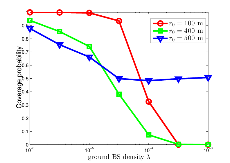
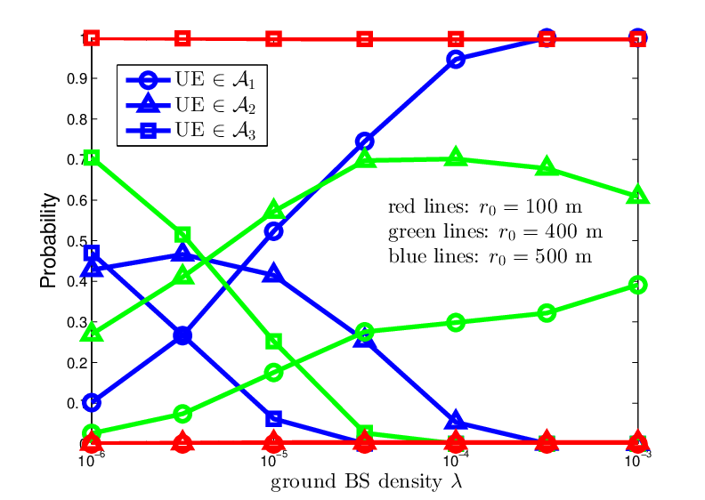
Fig. 6 studies the impact of the ground BS density on the performance of the proposed scheme. Fig. 6(a) shows the coverage probability versus for UEs with different locations, and Fig. 6(b) shows the probabilities of the events that the UE belongs to , and . As shown in the figure, when m, the UE is almost always served by the UAV only, thus the coverage probability deceases with due to the increased interference from ground BSs. It can also be seen from Fig. 6, when m, the coverage probability first decreases with and then maintains at about 0.5. This can be explained as follows. As shown in Fig. 6(b), at low , the UE belongs to and with high probability, in this case, the increasing interference from other ground BSs dominates the impact. While at high , the UE is only served by the nearest ground BS due to the very small distance. In this case, on the one hand, increasing results in decreasing the distance from the UE to the nearest ground BS which is positive to the coverage. On the other hand, increasing also results in increasing the interference from other ground BSs which is negative to the coverage. Consequently, the above two kinds of effect cancel each other and hence the coverage probability stays at a steady level.


Fig. 7 studies the impact of the cooperation parameter on the performance achieved by the proposed cooperative scheme and the benchmark scheme in [29] where UEs in the considered scenario are served by the mounted UAV only. From Fig. 7, we have the following observations. When m, the cooperation parameter has no effect on the coverage probability of the proposed scheme. Because the UE is almost sure to be served by the UAV only as shown in Fig. 7(b). This also explains the fact that the proposed scheme has the same performance as the benchmark scheme as shown in Fig. 7(a). When m and m, the coverage probabilities decrease with . For example, with m, decreases from to . This can be explained from Fig. 7(b) that as increases, the probability of the event that the UE belongs to decreases. As a result, it is more likely that the UE is served by the UAV only or the nearest ground BS only. It can also be seen from the figure that the proposed cooperative scheme always outperforms the benchmark scheme in terms of the coverage probability, even when which means the UE can only be served by a UAV or a nearest ground BS. This is because BS association is carried out when which is ignored in the benchmark scheme.


Fig. 8 shows the comparison between the proposed cooperative scheme and two benchmarks. In the benchmark scheme termed “UAV only”, the UE is served by the UAV, while in the scheme termed “ground BS only”, it is assumed that there is no UAV employed in the malfunction area and the UE is served by the nearest ground BS only. Fig. 8(a) shows the coverage probabilities versus the UE location . It is shown that when is small, the proposed scheme achieves similar performances compared to the “UAV only” scheme. While as increases, the proposed scheme outperforms the “UAV only” scheme. This can be explained as follows. When is small, the proposed scheme assigns the UE to with high probability, due to the very small distance to the UAV and the high probability of an LoS link. However, as increases, the channel between the UAV and the UE becomes weaker, after realizing this change, the proposed scheme automatically switches the transmission strategy according to expression (3) by assigning the UE to or , in order to provide better service compared to the “UAV only” scheme. It is also observed in Fig. 8(a) that the proposed scheme significantly outperforms the “ground BS only” scheme for most of . However, when approaches to , i.e., the UE locates at the edge of the malfunction area, the “ground BS only” achieves similar performance compared to the proposed scheme. Fig. 8(b) shows the NSE versus the radius of the circular malfunction area . From Fig. 8(b), is is shown that the proposed scheme outperforms the “UAV only” and the “ground BS only” scheme in terms of NSE. It is also observed that as increases, the NSEs achieved by the proposed scheme for different are the same.
V Conclusions
In this paper, a user-centric cooperative scheme has been proposed for a UAV assisted malfunction area which is surrounded by PPP modeled ground BSs. The probabilistic LoS/NLoS channel model has been taken into consideration to model the air-to-ground channels. Average received power has been used as a criterion to determine which transmission strategy should be applied to serve the UE, i.e., the UAV only, the nearest ground BS only, or both of them. A parameter has been introduced to tune the cooperation level of the proposed scheme. Analytical framework has been developed to evaluate the performance by developing the expressions for the coverage probability and NSE, which has been verified by computer simulations. Extensive numerical results have been presented to demonstrate the impact of different parameters on the performance achieved the proposed scheme. It has been shown that the proposed scheme has superior performance over the “UAV only” scheme in [29] and the “ground BS only” scheme.
Although the superiority of the proposed scheme has been demonstrated in this paper, there are still some important topics for future research about the application of UAVs to the considered malfunction area. For example, whether moving UAVs can provide better performance to such a scenario is still unknown. Besides, as the size of the malfunction area increases, it is not enough to utilize only one UAV in the malfunction area and it is necessary to deploy multiple UAVs.
Appendix A Proof for Lemma 1


Note that, since there’s no BS in disc , the value range of has to satisfy . To obtain the conditional pdf of , we need to first calculate the conditional CDF of , which is given by:
| (31) | ||||
where the last step follows from the fact that the BSs are HPPP distributed outside disc . Denote the disc centered at the UE with radius by , then in (31) is the area of the region which can be represented by .
- 1.
When , to calculate , we need to first calculate and . With the help of Fig. 9, it is obtained that can be expressed as follows:
(32) where . It is worth pointing out that, when changes, the value range of is .
Similarly, can be expressed as follows:
(33) where , and when changes, the value range of is also .
Then can be expressed as
(34) - 2.
When , can be easily obtained as follows:
(35)
Until now, we have obtained the conditional CDF of . By taking the derivative of , the conditional pdf of given can be obtained and the proof for Lemma 1 is complete.
Appendix B Proof for Lemma 2 and Lemma 3
B-A Proof for Lemma 2
The Laplace transform of can be calculated as follows:
| (36) | ||||
where the last step follows from the fact that the small scale fading gains are independently exponential variables with parameter .
By applying the probability generating functional (PGFL) of the HPPP, can be further expressed as follows:
| (37) |
where denotes the integration region which can be determined by both and . Note that, can be written as
| (38) |
where means that the distance from the UE to the interfering BS should be larger than that of the nearest BS, and means that the interfering BS should locate outside disc D.
Define
| (39) |
then the remaining task is to evaluate . By treating as the origin and changing to polar coordinates, can be expressed as follows:
| (40) |
where can be easily derived from and can be expressed as:
| (41) |
where is the length of as shown in Fig. 10, which can be easily obtained by the law of cosine. It is worth pointing out that the counterpart of the constraint in (22) is in (19).

According to the relevant relationship of and , the calculation of can be divided into the following two cases.
- 1.
Case I: . In this case, the integration region can be divided into two parts and , i.e., , as shown in Fig. 10. Mathematically, , and . Then can be evaluated as follows:
(42) where (a) follows from the step by using , and (b) follows from the application of Chebyshev-Gauss approximation.
- 2.
Case II: . In this case, as shown in Fig. 11, the integration region degrades to the following format . Then can be evaluated by following the similar steps as in Case I and the following expression for in Case II is obtained:
(43)

Now the proof for Lemma 2 is complete.
B-B Proof for Lemma 3
From the proof for Lemma 2, we know that can be expressed by the following integration:
| (44) |
Then exchanging the order of the derivative and integration, the -th derivative can be expressed as follows:
| (45) |
By dividing the calculation into the two cases as in the proof for Lemma 2 and following the similar steps as in (42) and (43), the expressions in (15) and (16) are obtained and the proof for Lemma 3 is complete.
Appendix C
C-A Proof for Proposition 1
can be evaluated as follows:
| (46) | ||||
where in (a), is a random variable which indicate whether the link from the UE to the UAV is an LoS or an NLoS link, and the probability of s is defined in (1), (b) follows by changing the order of the expectation and integration and then changing to polar coordinates, (c) and (d) follow by taking expectation with respect to and in sequence.
By following the same method, the expression for and can be obtained and the proof is complete.
C-B Proof for Corollary 1
Here, only the proof for the conclusion that increases with is provided. The other two conclusions can be proved by following similar steps.
To prove increasing with is equivalent to prove that increases with . Note that, when , , which has no contribution to . Thus it is necessary to rewrite the integration constraint in (17) as follows:
| (47) |
where when , otherwise is the root of the equation: . Note that it is easy to prove that the root always exists in .
Now in (47), the integral function is always positive and hence is an increasing function with . In this cases, it can be concluded that increases with , since increasing with . Further by noting that, for any , , the proof for increasing with is complete.
C-C Proof for Corollary 2
We only prove that increases with where the case that decreases with can be proved similarly.
Appendix D Proof for Lemmas -
- 1.
When , the conditional coverage probability can be calculated as follows:
(48) where (a) follows from the fact that is Rayleigh distributed and (b) follows from the fact that and are independent random variables. Finally, note that is a normalized Gamma distribution with parameter . Therefor, by applying the Laplace transform of given in Lemma 1, Lemma 4 is proved.
- 2.
When , the conditional coverage probability can be expressed as follows:
(49) To calculate , we need to obtain the CDF for . Note that, , it is easily obtained that
(50) Similarly, we have
(51) Then the Laplace transform for can be expressed as follows:
(52) where the last step follows from partial fraction decomposition. By taking the inverse Laplace transform, the CCDF for can be obtained as follows:
(53) Now the coverage probability can be expressed as follows:
(54) By further noting that , Lemma 5 is proved.
- 3.
When , the conditional coverage probability can be calculated as follows:
(55) where and the last step follows from that . By further noting that , Lemma 6 is proved.
References
- [1] K. P. Valavanis and G. J. Vachtsevanos, Handbook of unmanned aerial vehicles. Springer Publishing Company, Incorporated, 2014.
- [2] M. Asadpour, B. Van den Bergh, D. Giustiniano, K. A. Hummel, S. Pollin, and B. Plattner, “Micro aerial vehicle networks: An experimental analysis of challenges and opportunities,” IEEE Commun. Mag., vol. 52, no. 7, pp. 141–149, Jul. 2014.
- [3] Y. Zeng, R. Zhang, and T. J. Lim, “Wireless communications with unmanned aerial vehicles: opportunities and challenges,” IEEE Commun. Mag., vol. 54, no. 5, pp. 36–42, May 2016.
- [4] Z. Xiao, P. Xia, and X.-G. Xia, “Enabling UAV cellular with millimeter-wave communication: Potentials and approaches,” IEEE Commun. Mag., vol. 54, no. 5, pp. 66–73, May 2016.
- [5] H. Menouar, I. Guvenc, K. Akkaya, A. S. Uluagac, A. Kadri, and A. Tuncer, “UAV-enabled intelligent transportation systems for the smart city: Applications and challenges,” IEEE Commun. Mag., vol. 55, no. 3, pp. 22–28, Mar. 2017.
- [6] Y. Chen, N. Zhao, Z. Ding, and M.-S. Alouini, “Multiple UAVs as relays: Multi-hop single link versus multiple dual-hop links,” IEEE Trans. Wireless Commun., vol. 17, no. 9, pp. 6348–6359, Sep. 2018.
- [7] A. Merwaday, A. Tuncer, A. Kumbhar, and I. Guvenc, “Improved throughput coverage in natural disasters: Unmanned aerial base stations for public-safety communications,” IEEE Veh. Technol. Mag., vol. 11, no. 4, pp. 53–60, Dec. 2016.
- [8] S. Kandeepan, K. Gomez, L. Reynaud, and T. Rasheed, “Aerial-terrestrial communications: terrestrial cooperation and energy-efficient transmissions to aerial base stations,” IEEE Trans. Aerosp. Electron. Syst., vol. 50, no. 4, pp. 2715–2735, Oct. 2014.
- [9] S. Chandrasekharan, K. Gomez, A. Al-Hourani, S. Kandeepan, T. Rasheed, L. Goratti, L. Reynaud, D. Grace, I. Bucaille, T. Wirth et al., “Designing and implementing future aerial communication networks,” IEEE Commun. Mag., vol. 54, no. 5, pp. 26–34, May 2016.
- [10] M. Mozaffari, W. Saad, M. Bennis, and M. Debbah, “Mobile unmanned aerial vehicles (UAVs) for energy-efficient internet of things communications,” IEEE Trans. Wireless Commun., vol. 16, no. 11, pp. 7574–7589, Nov. 2017.
- [11] A. Merwaday and I. Guvenc, “UAV assisted heterogeneous networks for public safety communications,” in Proc. IEEE Wireless Commun. Networking Conf. Workshop (WCNCW). IEEE, Mar. 2015, pp. 329–334.
- [12] S. Jeong, O. Simeone, and J. Kang, “Mobile edge computing via a UAV-mounted cloudlet: Optimization of bit allocation and path planning,” IEEE Trans. Veh. Technol., vol. 67, no. 3, pp. 2049–2063, Mar. 2018.
- [13] D. W. Matolak and R. Sun, “Unmanned aircraft systems: Air-ground channel characterization for future applications,” IEEE Veh. Technol. Mag., vol. 10, no. 2, p. 79, Jun. 2015.
- [14] Q. Feng, J. McGeehan, E. K. Tameh, and A. R. Nix, “Path loss models for air-to-ground radio channels in urban environments,” in Proc. IEEE Veh. Technol. Conf. (VTC), Melbourne, Vic, Australia, May 2006, pp. 2901–2905.
- [15] J. Holis and P. Pechac, “Elevation dependent shadowing model for mobile communications via high altitude platforms in built-up areas,” IEEE Trans. Antennas Propagat., vol. 56, no. 4, pp. 1078–1084, Apr. 2008.
- [16] A. Al-Hourani, S. Kandeepan, and A. Jamalipour, “Modeling air-to-ground path loss for low altitude platforms in urban environments,” in Proc. IEEE Global Telecommun. Conf. (GLOBECOM), Austin, TX, USA, Dec. 2014, pp. 2898–2904.
- [17] A. Al-Hourani, S. Kandeepan, and S. Lardner, “Optimal LAP altitude for maximum coverage,” IEEE Wireless Commun. Lett., vol. 3, no. 6, pp. 569–572, Dec. 2014.
- [18] V. Sharma, M. Bennis, and R. Kumar, “UAV-assisted heterogeneous networks for capacity enhancement,” IEEE Commun. Lett., vol. 20, no. 6, pp. 1207–1210, Jun. 2016.
- [19] J. Xu, Y. Zeng, and R. Zhang, “UAV-enabled wireless power transfer: Trajectory design and energy optimization,” IEEE Trans. Wireless Commun., vol. 17, no. 8, pp. 5092–5106, Aug. 2018.
- [20] X. Pang, Z. Li, X. Chen, Y. Cao, N. Zhao, Y. Chen, and Z. Ding, “UAV-Aided NOMA Networks with Optimization of Trajectory and Precoding,” in Proc. WCSP 2018, Hangzhou, China, Oct. 2018, pp. 1–6.
- [21] J. Lyu, Y. Zeng, and R. Zhang, “Cyclical multiple access in UAV-aided communications: A throughput-delay tradeoff,” IEEE Wireless Commun. Lett., vol. 5, no. 6, pp. 600–603, Aug. 2016.
- [22] M. Haenggi, Stochastic Geometry for Wireless Networks. Cambridge, U.K.: Cambridge Univ. Press, 2012.
- [23] M. Mozaffari, W. Saad, M. Bennis, and M. Debbah, “Unmanned aerial vehicle with underlaid device-to-device communications: Performance and tradeoffs,” IEEE Trans. Wireless Commun., vol. 15, no. 6, pp. 3949–3963, Jun. 2016.
- [24] C. Zhang and W. Zhang, “Spectrum sharing for drone networks,” IEEE J. Select. Areas Commun., vol. 35, no. 1, pp. 136–144, Jan. 2017.
- [25] J. Ye, C. Zhang, H. Lei, G. Pan, and Z. Ding, “Secure UAV-to-UAV Systems with Spatially Random UAVs,” IEEE Wireless Commun. Lett., to be published.
- [26] V. V. Chetlur and H. S. Dhillon, “Downlink coverage analysis for a finite 3-D wireless network of unmanned aerial vehicles,” IEEE Trans. Commun., vol. 65, no. 10, pp. 4543–4558, Oct. 2017.
- [27] E. Turgut and M. C. Gursoy, “Downlink Analysis in Unmanned Aerial Vehicle (UAV) Assisted Cellular Networks with Clustered Users,” IEEE Access, vol. 6, pp. 36 313–36 324, May 2018.
- [28] X. Wang, H. Zhang, Y. Tian, and V. C. Leung, “Modeling and Analysis of Aerial Base Station Assisted Cellular Networks in Finite Areas under LoS and NLoS Propagation,” IEEE Trans. Wireless Commun., vol. 17, no. 10, pp. 6985–7000, Oct. 2018.
- [29] X. Wang, H. Zhang, and V. C. Leung, “Modeling and performance analysis of UAV-assisted cellular networks in isolated regions,” in Proc. IEEE Int. Conf. Commun Workshop (ICC Workshop), Kansas City, MO, USA, May 2018, pp. 1–6.
- [30] K. Feng and M. Haenggi, “A tunable base station cooperation scheme for poisson cellular networks,” in Proc. Conf. Inf. Sci. Syst. (CISS), Princeton, NJ, USA, Mar. 2018, pp. 1–6.