Average-case complexity of a branch-and-bound algorithm for min dominating set

Tom Denat, Ararat Harutyunyan, Vangelis Th. Paschos
Université Paris-Dauphine, PSL* Research University, CNRS UMR 7243, LAMSADE, Paris 75016, France
{tom.denat,ararat.harutyunyan,vangelis.paschos}@lamsade.dauphine.fr

Abstract

The average-case complexity of a branch-and-bound algorithms for min dominating set problem in random graphs in the $\mathcal{G}(n,p)$ model is studied. We identify phase transitions between subexponential and exponential average-case complexities, depending on the growth of the probability $p$ with respect to the number $n$ of nodes.

1 Introduction

Given a graph $G=(V,E)$ of order $n$ , a dominating set $S\subseteq V$ is a subset of $V$ such that any $v_{i}\in V$ is either included in $S$ or connected to a vertex of $S$ by an edge of $E$ . The min dominating set problem consists of finding a minimum-size dominating in $G$ . min dominating set is a very well-known NP-hard problem completely equivalent (from both complexity and polynomial approximation points of view) to min set cover problem.

Dealing with the exact solution of min dominating set, besides the obvious $O(2^{n})$ algorithm which considers the power set of $V$ and chooses the smallest one that also forms a dominating set, several moderately exponential algorithms have been proposed mainly during the last fifteen years. To the best of our knowledge, the fastest one is the $O(1.4969^{n})$ algorithm due to [7].

The main purpose of this paper is the study of the average case complexity of branch-and-bound algorithms for the min dominating set problem in random graphs in the $\mathcal{G}(n,p)$ model. This model represents graphs on $n$ vertices where each of the possible $\binom{n}{2}$ edges appears independently with probability $p$ . For an extensive treatment of random graphs, we refer the reader to the monograph [3].

Even though branch-and-bound is one of the best known and most widely used techniques for exactly solving NP-hard problems, there has been little systematic study of its complexity, worst- or average case. Also, even though mathematical tools for average case analysis of algorithms have existed for decades [6] and have much advanced in sophistication [5], we do not know of many results on the average case complexity of exact algorithms for NP-hard problems. The only works known to us are the ones of [2] where the authors study the complexity of a “pruning the search-tree algorithm" for max independent set (the worst-case complexity of this algorithm is $O(1.3803^{n})$ , [8]) under the $\mathcal{G}(n,p)$ model, the one of [1], where the same algorithm is studied under the $\mathcal{G}(n,m)$ model and, finally, the one in [4] where the average-case complexity of a branch-and-bound algorithm for max independent set is studied under the $\mathcal{G}(n,p)$ model.

In what follows, in Section 2 we specify the branch-and-bound algorithm the complexity of which is then analysed in Section 3. Finally, in Section 4 we study the complexity of simple exhaustive search algorithm which, starting from the whole vertex-set $V$ of the input graph, produces a minimum dominating set by considering all the subsets of $V$ and finally returns the smallest one that is a dominating set.

2 The branch-and-bound algorithm

Let $G=(V,E)$ be a graph; set $n=|V|$ and fix an order $v_{1},v_{2},\ldots,v_{n}$ on $V$ . The type of branch-and-bound algorithms for min dominating set studied here works by building a branch-and-bound binary tree, nodes of which are associated with a vector $\vec{x}\in\{0,1\}^{n}$ and a depth $\delta$ in the binary tree. Obviously, $x_{i}=1$ means that vertex $v_{i}$ has been taken in the solution under construction and $x_{i}=0$ means that $v_{i}$ has not been taken. For a tree-node at level $\delta$ only vertices $v_{1},v_{2},\ldots,v_{\delta}$ have been explored, i.e., only $x_{1},x_{2},\ldots,x_{\delta}$ have been assigned definite values. At this point the values for $x_{\delta+1},\ldots,x_{n}$ are, for the moment, equal to 1. We remark that the superset of a dominating set is also a dominating set.

The root of the branch-and-bound tree $T$ corresponds to the trivial dominating set including all the vertices ( $\vec{x}=(1,1,...,1)$ ) at the depth 0 and is initially visited. The left child $(\vec{x},\delta)_{l}=(\vec{x},\delta+1)$ of a node $n_{i}=(\vec{x},\delta)$ at level $\delta$ of $T$ , has exactly the same vector $\vec{x}$ as $n_{i}$ but with the value of $x_{\delta+1}=1$ now determined, i.e., the partial solution represented by $n_{i}$ is extended by putting $v_{\delta+1}$ in the solution under construction. The right child $(\vec{x},\delta)_{r}$ of $(\vec{x},\delta)$ corresponds to changing the partial solution represented by $n_{i}$ by putting $x_{\delta+1}=0$ .

At each new step of the algorithm a new node will be explored. In order to be explorable a node $(\vec{x},\delta)$ must correspond to a dominating set in $G$ and be either the left or the right child of an already visited node.

Therefore, at each step of the algorithm, the nodes can be divided in four categories:

1.

the already visited nodes which correspond to dominating sets (feasible solutions);
2.

the nodes that correspond to vertex-sets that are not dominating sets in $G$ (the infeasible solutions);
3.

the explorable solutions which correspond to dominating sets in $G$ and are either the left or the right child of an already visited node;
4.

the currently “hidden” feasible solutions which correspond to dominating sets in $G$ but are not the left nor the right child of an already visited node.

For a node at level $\delta$ with vector $\vec{x}$ , we define its score $u(\vec{x},\delta)$ as the number of vertices that currently must be included in the solution. Formally:

u\left(\vec{x},\delta\right)=\left|\vec{x}\right|-n+\delta

where $|\vec{x}|=\sum_{i=1,2,\ldots n}x_{i}$ . Score $u(\vec{x},\delta)$ can be seen as an optimistic prediction of the value of the optimal solution since it implies that no other vertex will be added to the feasible solution corresponding to the node at hand.

The choice of the next node to be explored among the explorable nodes (solutions) is made by minimizing a score $u(\vec{x},\delta)$ , named potential in what follows, associated with each node of the branch-and-bound tree.

The explorable solutions corresponding to tree-nodes of depth $n$ constitute feasible dominating sets for the whole $G$ . It is easy to see that the leftmost among them corresponds to a minimum dominating set of $G$ .

Refer to caption — Figure 1: Illustration of the branch-and-bound algorithm for the minimum dominating set problem. The instance $G$ appears on the upper left corner of the figure. In the branch-and-bound tree, the nodes representing feasible solutions are coloured in deep blue. The green number above each node represents the score function $u(\vec{x})$ .

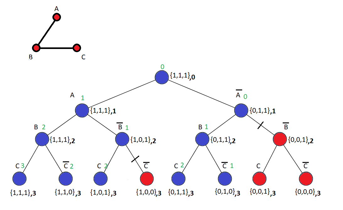
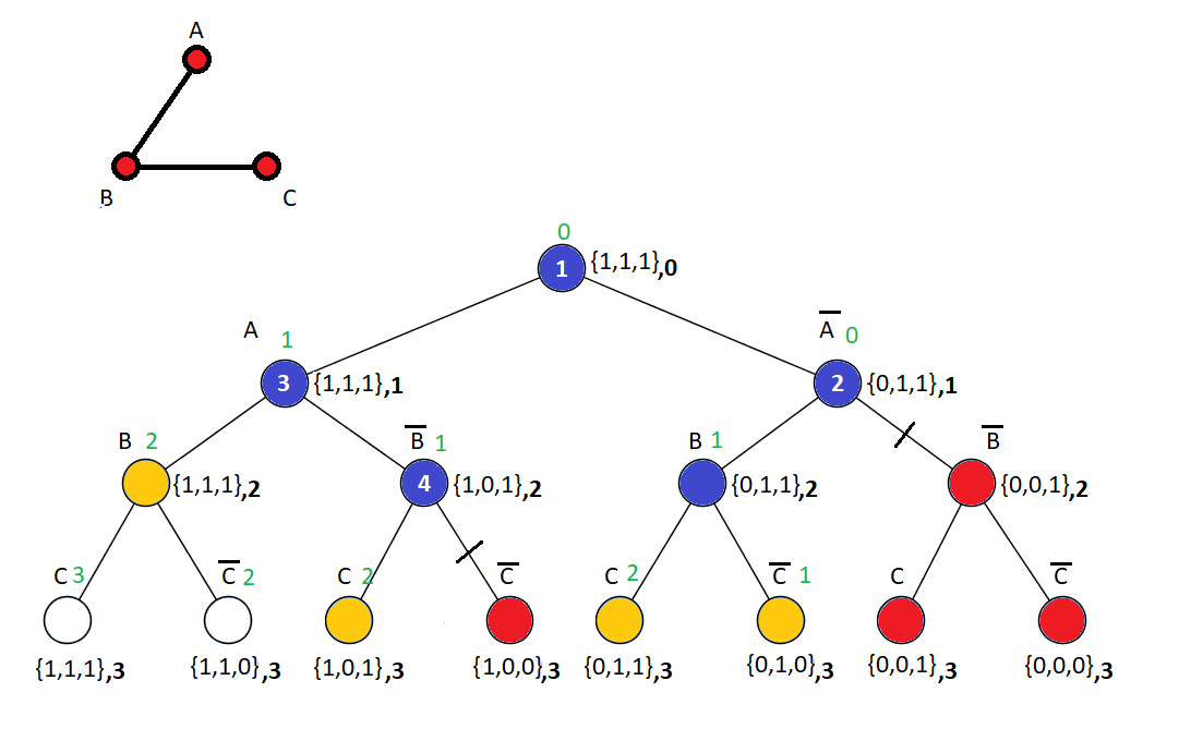
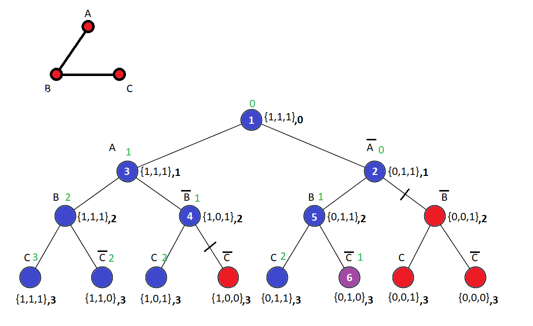
As an example, on figure 1 the graph $G$ contains three vertices $A$ , $B$ and $C$ . Therefore, the branch-and-bound tree contains 3 levels. The branch and bound algorithm starts by exploring the root $\{1,1,1\},0$ . Now, the explorable nodes are $\{1,1,1\},1$ and $\{0,1,1\},1$ with respective potentials $1$ and $0$ . Therefore, the node $\{0,1,1\},1$ is explored next. Then, the two explorable nodes are $\{1,1,1\},1$ and $\{0,1,1\},2$ , both with potential $1$ . The next node to be explored is chosen randomly. Assume that the next explored node is $\{1,1,1\},1$ and so on. Finally, the complete solution $\{0,1,0\},3$ is found. As its depth is 3, this solution $\{B\}$ is the minimum dominating set.

In what follows, we denote by $\mathbb{T}(n,p)$ the average complexity of branch-and-bound in a binomial random graph $G=(V,E)$ with parameters $(n,p)$ , that is, the total number of leaves expansions, and by $\mathbb{E}[\#S(G)]$ the expectation of the number of dominating sets in a binomial random graph $G$ .

3 Analysis of the branch-and-bound algorithm

Notice first that any child $xb$ of a node $x$ of the branch and bound tree, where $b\in\{0,1\}$ , has $u(xb)\geqslant u(x)$ .

So, let $x$ be the first leaf at the $n$ th level — that is with $|x|=n$ — expanded by the algorithm; obviously $u(x)=|S_{x}|$ . Any leaf that has not been expanded yet must have a bound that is at least $|S_{x}|$ (otherwise they would have been handled before). Since all other unexpanded leaves have bounds no smaller than $|S_{x}|$ , $S_{x}$ must be a minimum dominating set, and the algorithm terminates.

It follows that, during the running of the algorithm, a leaf $x$ is expanded only if $u(x)\leqslant|S^{*}|$ , where $S^{*}$ is the minimum dominating set. Thus, the expanded leaves $x$ with $|x|=i$ are dominating subsets $S\subseteq\{1,\ldots,i\}$ satisfying $n-|S|\leqslant|S^{*}|$ . We can therefore write:

$\displaystyle\mathbb{T}$	$\displaystyle\leqslant$	$\displaystyle\sum\limits_{i=0}^{n}\sum\limits_{S\subseteq\{1,2,\ldots,i\}}\mathbb{P}\left((\text{$S$ is a dominating set})\cap\left(n-\|S\|\leqslant\left\|S^{*}\right\|\right)\right)\Rightarrow$
$\displaystyle\Rightarrow\mathbb{T}$	$\displaystyle\leqslant$	$\displaystyle\sum\limits_{i=0}^{n}\sum\limits_{S\subseteq\{1,2,\ldots,i\}}\mathbb{P}\left(\text{$S$ is a dominating set}\right)\;\;\wedge\;\;\mathbb{T}\leqslant\sum\limits_{i=0}^{n}\sum\limits_{S\subseteq\{1,2,\ldots,i\}}\mathbb{P}\left(n-\|S\|\leqslant\left\|S^{*}\right\|\right)$	(1)
	$\displaystyle\leqslant$	$\displaystyle n\cdot\max_{1\leqslant k\leqslant n}\binom{n}{k}\Pr[\gamma>n-k]$	(1)

Thus, we need to upper-bound the quantity $M:=\binom{n}{k}\Pr[\gamma>n-k]$ for all $1\leqslant k\leqslant n$ .

3.1 Upper bounds

The following theorem provides upper bounds for the complexity of the branch-and-bound algorithm presented in Section 2 for random graphs in the $\mathcal{G}(n,p)$ model.

Theorem 1.

The following two facts hold:

(a)

If $pn\to\infty$ , then the branch-and-bound algorithm takes subexponential time.
(b)

If $pn=c$ , where $c\geqslant 20$ is a constant, then the branch-and-bound algorithm takes time $(2-\epsilon)^{n}$ , where $\epsilon\geqslant 0.01$ is some constant.

Proof.

We first focus on the case where $p$ is fixed. We show that in this case, $M$ is subexponential. We use the fact that $\gamma(G)\leqslant\alpha(G)$ for every graph $G$ , where $\alpha(G)$ denotes the stability number of graph $G$ (indeed, a maximal independent set is a dominating set) and the union bound.

We recall that $1-x\leqslant e^{-x}$ for all values of $x$ ( this follows from the fact that $1-x$ is the tangent line of $e^{-x}$ at $x=0$ ). We remark that $\alpha(G)>x$ for some $x$ , implies that one of the $\binom{n}{x}$ subsets of vertices of size $x$ induces an independent set in $G$ . Thus:

M\leqslant\binom{n}{k}\Pr[\alpha>n-k]\leqslant\binom{n}{k}\binom{n}{n-k}(1-p)^{\binom{n-k}{2}}\leqslant\left(\binom{n}{n-k}\right)^{2}e^{\nicefrac{{-p(n-k)(n-k-1)}}{{2}}}=\binom{n}{x}^{2}e^{-\nicefrac{{px(x-1)}}{{2}}}

where $x=n-k$ . We consider $x$ as a function of $n$ , setting $x:=f(n)$ . If $f(n)=o(n)$ , then $\binom{n}{x}^{2}<(\nicefrac{{en}}{{x}})^{2x}$ is clearly subexponential. Thus, we may assume $f(n)=\Theta(n)$ . Quantity $M$ clearly satisfies:

M\leqslant\left(\left(\frac{en}{x}\right)^{2}e^{\nicefrac{{-p(x-1)}}{{2}}}\right)^{x}

Since $f(n)=\Theta(n)$ and $p$ is fixed, clearly, $(\nicefrac{{en}}{{x}})^{2}e^{\nicefrac{{-p(x-1)}}{{2}}}<1$ for $n$ sufficiently large. In fact, with a slightly more careful analysis, we can obtain that $M$ is subexponential in the regime $pn\to\infty$ . Indeed, we may suppose as before that $x=\Theta(n)$ and now it follows that $(\nicefrac{{en}}{{x}})^{2}$ is bounded by a constant and since $p=\omega(1)$ we have that $e^{-\nicefrac{{p(x-1)}}{{2}}}\to 0$ , as $n\to\infty$ . Therefore, $(\nicefrac{{en}}{{x}})^{2}e^{-\nicefrac{{p(x-1)}}{{2}}}<1$ for $n$ sufficiently large and the claim follows.

It remains to consider the case (b), where $p=\nicefrac{{c}}{{n}}$ , where $c\geqslant 20$ is some absolute constant. As before, we consider the quantity $\binom{n}{x}^{2}e^{\nicefrac{{-px(x-1)}}{{2}}}$ . We may assume as before that $x=\Omega(n)$ , i.e. $\lim_{x\to\infty}\nicefrac{{x}}{{n}}=\epsilon$ , for some $\epsilon>0$ . Indeed, otherwise the time is subexponential. Thus, we need to show that $\binom{n}{\epsilon n}^{2}(1-p)^{\nicefrac{{\epsilon^{2}n^{2}}}{{2}}}$ is bounded for any $\epsilon>0$ . We use the fact that $\binom{n}{\epsilon n}=2^{(1+o(1))H(\epsilon)n}$ , where $H(\epsilon)$ is the binary entropy function. Thus,

\binom{n}{\epsilon n}^{2}(1-p)^{\nicefrac{{\epsilon^{2}n^{2}}}{{2}}}\leqslant\left(\left[\left(\epsilon^{-\epsilon}(1-\epsilon)^{-(1-\epsilon)}\right)^{(1+o(1))}\right]^{2}e^{-c\nicefrac{{\epsilon^{2}}}{{2}}}\right)^{n}

We remark that $(\epsilon^{-\epsilon}(1-\epsilon)^{-(1-\epsilon)})$ is increasing on the interval $(0,\nicefrac{{1}}{{2}})$ and decreasing on $(\nicefrac{{1}}{{2}},1)$ , with its maximum at $\epsilon=\nicefrac{{1}}{{2}}$ , since $H(\epsilon)$ is the logarithm of this function. Thus, there is some constant $\epsilon_{0}<\nicefrac{{1}}{{2}}$ such that, for all $\epsilon\leqslant\epsilon_{0}$ , $(\epsilon^{-\epsilon}(1-\epsilon)^{-(1-\epsilon)})<\sqrt{2}$ . It is easy to check that we can take $\epsilon_{0}=\nicefrac{{1}}{{10}}$ . Thus, we may assume that $\epsilon>\nicefrac{{1}}{{10}}$ . Since $c\geqslant 20$ , it suffices to show that:

\left[\left(\epsilon^{-\epsilon}(1-\epsilon)^{-(1-\epsilon)}\right)^{(1+o(1))}\right]^{2}e^{-10\epsilon^{2}}<2

for all $\epsilon\in[\nicefrac{{1}}{{10}},\nicefrac{{1}}{{2}}]$ . Since the first of the two products is increasing and the second is decreasing with $\epsilon$ , we will have to dominate each separately. To this end, we refine the intervals of $\epsilon$ . First consider the interval $\epsilon\in[\nicefrac{{1}}{{10}},\nicefrac{{1}}{{8}}]$ . To bound our product, it is sufficient to substitute $\nicefrac{{1}}{{8}}$ in the first term and $\nicefrac{{1}}{{10}}$ in the second. By doing this, we obtain that the product is less than, say, 1.99. It is easily verified that we can repeat this argument on the following intervals, thus finishing the theorem. In each case, we obtain a bound of less than 1.99. The precise bounds are given below, where $f(\epsilon):=[(\epsilon^{-\epsilon}(1-\epsilon)^{-(1-\epsilon)})^{(1+o(1))}]^{2}e^{-10\epsilon^{2}}$ :

•

$\epsilon\in[1/8,1/7];f(\epsilon)<1.943$ ;
•

$\epsilon\in[1/7,0.15];f(\epsilon)<1.9$ ;
•

$\epsilon\in[0.15,0.17];f(\epsilon)<1.988$ ;
•

$\epsilon\in[0.17,0.19];f(\epsilon)<1.981$ ;
•

$\epsilon\in[0.19,0.21];f(\epsilon)<1.95$ ;
•

$\epsilon\in[0.21,0.25];f(\epsilon)<1.982$ ;
•

$\epsilon\in[0.25,0.35];f(\epsilon)<1.955$ ;
•

$\epsilon\in[0.35,0.5];f(\epsilon)<1.2$ .

The proof of the theorem is now completed. ∎

3.2 Lower bounds

The following result shows that the upper bound on complexity of the algorithm given by Item (b) of Theorem 1 cannot be drastically improved in order that a subexponential bound is taken.

Theorem 2.

Let $p=\nicefrac{{c}}{{n}}$ , where $c$ is a positive fixed constant. Then, the branch-and-bound algorithm takes at least $(\nicefrac{{1}}{{\epsilon}})^{\epsilon n}$ time for $G(n,p)$ , where $\epsilon:=\max\{0.99,1-(\nicefrac{{1}}{{10c}})\}$

Proof.

It is sufficient to show that:

\binom{n}{\epsilon n}\Pr[\gamma>n-\epsilon n]=\Omega\left(\left(\frac{1}{\epsilon}\right)^{\epsilon n}\right)

for $n$ sufficiently large.

We will prove that $\Pr[\gamma\leqslant n-\epsilon n]$ is arbitrarily small. This is clearly sufficient. Let $A$ be the event that a fixed set $S$ of size $n-\epsilon n$ is a dominating set. Then, $\Pr[\gamma\leqslant n-\epsilon n]\leqslant\binom{n}{n-\epsilon n}\Pr[A]<2^{n}\Pr[A]$ . We use the fact that $1-x\geqslant e^{-2x}$ for all $x\in(0,\nicefrac{{1}}{{2}})$ ; this can be seen, for example, by noticing that $e^{-2x}$ is a convex function and that $1-x=e^{-2x}$ has two solutions at $x=0$ and at some $x\in(0.5,1)$ . Now, $\Pr[A]=\left(1-(1-p)^{n-\epsilon n}\right)^{\epsilon n}\leqslant(1-e^{-2c(1-\epsilon)})^{\epsilon n}$ . Thus:

\Pr[\gamma\leqslant n-\epsilon n]\leqslant\left(2\left(1-e^{-2c(1-\epsilon)}\right)^{\epsilon}\right)^{n}

Now, if $c<10$ , then $(1-e^{-2c(1-\epsilon)})^{\epsilon}<(1-e^{-\nicefrac{{1}}{{5}}})^{0.99}<1/2$ . Similarly, if $c\geqslant 10$ , then $(1-e^{-2c(1-\epsilon)})^{\epsilon}<(1-e^{-\nicefrac{{1}}{{5}}})^{1-\nicefrac{{1}}{{10c}}}<1/2$ . Thus, $\Pr[\gamma\leqslant n-\epsilon n]<\delta^{n}$ , for some $\delta<1$ .

It follows that:

\binom{n}{\epsilon n}\Pr[\gamma>n-\epsilon n]=\Omega\left(\left(\frac{1}{\epsilon}\right)^{\epsilon n}\right)

as required. ∎

4 Analysis of the simple exhaustive search algorithm

We conclude the paper by studying in this section a simple exhaustive search algorithm which, starting from the whole vertex-set $V$ of the input graph produces a minimum dominating set by considering all the subsets of $V$ and finally returns the smallest one that is a dominating set. In the remaining part of this section, we prove the following proposition.

Proposition 1.

Consider a random $(n,p)$ -binomial graph $G$ . Then the following hold:

1.

if $p$ is smaller than $\nicefrac{{1}}{{n}}$ , then the complexity of the exhaustive search algorithm is subexponential;
2.

if $p=\nicefrac{{c}}{{n}}$ , for some constant $c>1$ , then:

$\mathbb{T}(n,p)\leqslant\max\left\{1.99^{n},\left(2\left(1-e^{-2c}\right)^{1/3}\right)^{n}\right\}$

Proof.

We first prove item 1. Consider a random $(n,p)$ -binomial graph $G$ . Recall that by definition of the $(n,p)$ -binomial random model, the probability that a set of which $k$ vertices are excluded is a dominating set of $G$ is equal to $(1-(1-p)^{n-k})^{k}$ ; henceforth:

\mathbb{E}[\#S(G)]=\sum_{k=0}^{n}{n\choose k}\left(1-(1-p)^{n-k}\right)^{k}\leqslant n\cdot\max\limits_{k\leqslant n}\left\{{n\choose k}(1-(1-p)^{n-k})^{k}\right\}

(3)

The number of dominating sets in the sub-graph induced by the $\alpha$ first fixed vertices is strictly greater than the number of dominating sets induced in the $\alpha-1$ first such vertices (since the $\alpha$ -th vertex is a dominating set by itself); so, using (3):

\mathbb{T}(n,p)\leqslant n\cdot\mathbb{E}[\#S(G)]\leqslant n\sum_{k=0}^{n}{n\choose k}\left(1-(1-p)^{n-k}\right)^{k}\leqslant n^{2}\cdot\max\limits_{k\leqslant n}\left\{{n\choose k}(1-(1-p)^{n-k})^{k}\right\}

(4)

Obviously, the more the edges in the graph the more likely is that a sub-graph is a dominating set and therefore the probability that a sub-graph is a dominating set increases with $p$ and decreases with $q=1-p$ . Let us consider the case $p=\nicefrac{{j}}{{n}}$ . We will thereafter consider that $k\sim in$ with $0<i<1$ . Indeed, when $k<in,\forall i>0$ (resp. $k>in,\forall i<1$ ) then ${n\choose k}$ is at most subexponential. Hence, the probability for a graph of size $n-k$ to be a dominating set is:

\left(1-\left(1-\frac{j}{n}\right)^{(1-i)n}\right)^{in}

which when $n$ tends to infinity tends to $(1-e^{j(i-1)})^{in}$ .

Using (4), discussion just above leads to:

\mathbb{T}(n,p)\leqslant n^{2}\cdot\max\limits_{0\leqslant i\leqslant 1}\left\{{n\choose in}(1-e^{j(i-1)})^{in}\right\}\leqslant n^{2}\cdot\max\limits_{0\leqslant i\leqslant 1}\left\{\frac{e^{in}}{i^{in}}(1-e^{j(i-1)})^{in}\right\}

(5)

Let $f(x)=(\nicefrac{{e^{x}}}{{x^{x}}})(1-e^{j(x-1)})^{x}$ . Then:

f^{\prime}(x)=-e^{x}\left(\frac{1}{x}\right)^{x}\left(1-e^{j(x-1)}\right)^{x-1}\left(\left(e^{j(x-1)}-1\right)\left(\log\left(1-e^{j(x-1)}\right)-\log(x)\right)\right)

which gives: $f^{\prime}(x)=0\Leftrightarrow 1-e^{j(x-1)}=x\Leftrightarrow x=1-(\nicefrac{{W(j)}}{{j}})$ . So:

\max\limits_{0\leqslant x\leqslant 1}f(x)=f\left(1-\frac{W(j)}{j}\right)=e^{1-\frac{W(j)}{j}}

where $W(\cdot)$ denotes the Lambert’s function defined by $x=W(x)e^{W(x)}$ . Let $g_{+}(j)=e^{1-(\nicefrac{{W(j)}}{{j}})}$ . Then, using (5), we get: $\mathbb{T}(n,p)\leqslant n^{2}\cdot g_{+}(j)^{n}$ .

Note that $g_{+}(0)=1$ and $\lim_{x\to\infty}g_{+}(x)=e$ . Then:

\mathbb{T}(n,p)\geqslant\max\limits_{0\leqslant i\leqslant 1}\left\{{n\choose in}(1-e^{j(i-1)})^{in}\right\}\geqslant\max\limits_{0\leqslant i\leqslant 1}\left\{\frac{1}{(i)^{in}}(1-e^{j(i-1)})^{in}\right\}\geqslant\exp\left(\frac{1}{e}-\left(\frac{W\left(je^{-j-1+\frac{j}{e}}\right)}{j}\right)\right)^{n}=g_{-}^{n}(x)

Observe that $\lim_{x\to\infty}g_{-}(x)=e^{\nicefrac{{1}}{{e}}}\simeq 1.44$ .

Given that the complexity of the exhaustive search algorithm is increasing with $p$ , discussion above concludes that it is subexponential if and only if $p$ is smaller than $\nicefrac{{1}}{{n}}$ and the proof of item 1 is now complete.

We now prove item 2. Here, we can clearly suppose $n/3<k<2n/3$ ; otherwise $\binom{n}{k}\leqslant 1.99^{n}$ and we are done. Using the fact that $1-x\geqslant e^{-2x}$ for $x\in(0,0.5)$ , one can deduce:

	$\displaystyle\mathbb{T}(n,p)$	$\displaystyle\leqslant$	$\displaystyle 2^{n}n^{2}\max\limits_{\nicefrac{{n}}{{3}}\leqslant k\leqslant\nicefrac{{2n}}{{3}}}\left\{{n\choose k}\left(1-(1-p)^{n-k}\right)^{k}\right\}$
		$\displaystyle\leqslant$	$\displaystyle 2^{n}n^{2}\left(1-\left(1-\frac{c}{n}\right)^{\nicefrac{{2n}}{{3}}}\right)^{\nicefrac{{n}}{{3}}}\;\;\leqslant\;\;2^{n}n^{2}\left(1-e^{-\nicefrac{{4c}}{{3}}}\right)^{\nicefrac{{n}}{{3}}}\;\;\leqslant\;\;n^{2}\left(2\left(1-e^{-\nicefrac{{4c}}{{3}}}\right)^{\nicefrac{{1}}{{3}}}\right)^{n}$

and the result for item 2 follows immediately. ∎

5 Conclusion

We have studied in this paper the average-case complexity of a branch-and-bound algorithm for min dominating set in random graphs under the $\mathcal{G}(n,p)$ model. It has been proved that this complexity is: (a) subexpontial when $p=\nicefrac{{f(n)}}{{n}}$ , for any function $f\rightarrow\infty$ with $n$ ; (b) exponential when $p=\nicefrac{{c}}{{n}}$ . For the latter case it was proved that the smaller the constant $c$ the closer to $2^{n}$ average case complexity of the algorithm. Then the complexity of a naive exhaustive search algorithm has been studied. Here, for $p$ smaller than $\nicefrac{{1}}{{n}}$ the algorithm is subexponential, while for $p\geqslant\nicefrac{{c}}{{n}}$ , $c>1$ , its complexity becomes exponential, tending, for very large values of $c$ , to $2^{n}$ .

References

[1] C. Banderier, H. Hwang, V. Ravelomanana, and V. Zacharovas. Average case analysis of NP-complete problems: maximum independent set and exhaustive search algorithms. International Meeting on Probabilistic, Combinatorial, and Asymptotic Methods in the Analysis of Algorithms, AofA09, 2009.
[2] C. Banderier, H. Hwang, V. Ravelomanana, and V. Zacharovas. Analysis of an exhaustive search algorithm in random graphs and the $n^{c\log n}$ -asymptotics. SIAM J. Disc. Math., 28(1):342–371, 2014.
[3] B. Bollobás. Random graphs. Academic Press, London, 1985.
[4] N. Bourgeois, R. Catellier, T. Denat, and V. Th. Paschos. Average-case complexity of a branch-and-bound algorithm for maximum independent set, under the $mathcal\{G\}(n,p)$ random model. CoRR, abs/1505.04969, 2015.
[5] Ph. Flajolet and R. Sedgewick. Analytic combinatorics. Cambridge University Press, 2008.
[6] D. E. Knuth. The art of computer programming: fundamental algorithms, volume 1. Addison-Wesley, Reading MA, 1969.
[7] J. M.M. van Rooij and H. L. Bodlaender. Exact algorithms for dominating set. Discrete Appl. Math., 159(17):2147–2164, 2011.
[8] G. J. Woeginger. Exact algorithms for NP-hard problems: a survey. In M. Juenger, G. Reinelt, and G. Rinaldi, editors, Combinatorial Optimization - Eureka! You shrink!, volume 2570 of Lecture Notes in Computer Science, pages 185–207. Springer-Verlag, 2003.