Singularity Free Direct Calculation of
Spontaneous Mass GenerationPreprint: KANAZAWA-18-08

Owing to its outstanding feature that it is the central issue of the elementary particle physics, dynamical chiral symmetry breaking phenomena have been widely studied using various methods. The standard method to discuss the spontaneous mass generation is to formulate a coupled system of self-consistent equations and find its non-trivial solution. However, those equations are no more than the necessary condition and it is needed to examine solutions to select correct one by using another means, e.g., by referring to the free energy of each solution. Even if it is done, it is still not completely clear whether the minimal free energy solution ensures the physically correct answer.

The method of setting up self-consistent equations for some infinite summation is based on the observation that the whole (T) resides in the whole as a part P. There must be a function $f$ that the whole is calculated by using the part,

$$T=f(P).$$

(1)

Then we have a self-consistent equation,

$$T=f(T),$$

(2)

and try to find solutions of this equation. Usually there are many solutions and we must proceed to pick up the physically correct one, supposing it is there anyway.

In contrast to the self-consistent equation method, we propose another method of iteration. We define a series of parts $P^{(n)}$, numbered by $n$, so that it has a feature:

$$\lim_{n\rightarrow\infty}P^{(n)}=T.$$

(3)

If we find an iterative relation,

$$P^{(n+1)}=F(P^{(n)}),$$

(4)

then the whole $T$ is given by a result after infinite iterations with the proper initial condition $P^{(0)}$. In this article, we set up this type of iterative method to calculate the spontaneous mass generation. As for the simplest toy example, see the Appendix A where the sum of geometric series is treated in this line of thought, which gives a clear view of our strategy.

Using the iterative method we can evaluate directly the spontaneously generated mass. This is absolutely non-trivial, since the spontaneous mass generation is nothing but the spontaneous symmetry breakdown of the chiral symmetry and it is an issue of phase transition. Phase transition of system is characterized by appearance of singularity and normally we have to make bypasses or deep consideration to evaluate physical quantities related to the phase transitionSSB.

The only escape is that if we can regularize the system a la finite volume (finite number of degrees of freedom), then there is no singularity, nothing unphysical, in any stage of regularization. We take the infinite volume limit at the last of calculation, which finally generates singularities in physical quantities and through such singularities, we obtain physically correct results, like the spontaneously generated mass.

Actually, our method described in this article can be regarded as a sort of this type of regularization realizing singularity free direct calculation. The part $P^{(n)}$ is a regularized quantity where $n$ represents the regularization parameter. Moreover our $P^{(n)}$ has a good physical feature that it assures the positivity of fluctuation at any $n$, which is easily lost in other approximation methods treating the spontaneous symmetry breakdown.

In Section 2, we set up the iterative summing up method of the all relevant diagrams to give the dynamical mass in the Nambu–Jona-Lasinio model. In Section 3, we show the spontaneous mass generation mechanism in this method and the results give the correct physical mass. In Section 4, we apply the iterative method to calculate various physical functions. As for the Legendre effective potential, we obtain the convex function automatically. In Section 5, we extend out method to the finite density system, where the 1st order phase transition is expected to occur. We find that our iteration fails to select the proper physical mass for some special regions of parameters. In Section 6, we treat the gauge theory and construct the similar iterative method to sum up all ladder type diagrams, which works well to give the spontaneously generated mass.

In this section, we adopt the Nambu–Jona-Lasinio (NJL) modelnambu and give a new iterative method that directly sums up an infinite number of diagrams of the standard perturbation theory in the bubble tree ($1/N$ leading) approximation. Using this method, we demonstrate that the physically correct result is automatically obtained with the precise critical coupling constant.

The NJL model has four-fermi interactions among the massless fermions respecting the chiral invariance. We add the bare mass $m_{0}\bar{\psi}\psi$ (explicitly breaking the chiral symmetry) to the Lagrangian to make the standard perturbation theory work properly,

$${\mathcal{L}}_{\rm{NJL}}=\bar{\psi}i{\vtop{\halign{#\cr\hfil/\hfil\crcr$\partial$\crcr}}}\psi+\frac{G}{2N}\left[\left({\bar{\psi}\psi}\right)^{2}+\left(\bar{\psi}i\gamma_{5}\psi\right)^{2}\right]-m_{0}\bar{\psi}\psi,$$

(5)

where $N$ is the number of fermion flavors. This model is not renormalizable and we set the ultraviolet cutoff $\Lambda$. The critical coupling constant for the spontaneous mass generation is $G=4\pi^{2}$ and we also use the rescaled coupling constant $g=G/(4\pi^{2})$.

We consider $1/N$ leading contribution to the mass. Diagrammatically it is a sum of infinite diagrams called tree (Fig.1), where considering the fermion-antifermion pair as a single meson, the tree diagrams are defined by those without any meson loops, or in other words we regard a series of loops as a fat propagator. Usual method is to set up a self-consistent equation satisfied by this infinite sum of diagrams.

Above the critical coupling constant, there actually exists a non-trivial solution which does not vanish after zero bare mass limit. However, it is unclear that how the finite mass should come out of the infinite sum of the diagrams while each diagram certainly vanishes at the zero bare mass limit. Now, we set up a method to directly sum up the infinite number of diagrams and show how the finite mass come out without any ambiguity nor singularity.

In the tree type diagrams drawn in Fig.1, we can easily find the whole sum resides as a part of the set. The part surrounded by a line is equivalent to the whole sum. This observation leads to the well-known self-consistent equation given by the original Nambu–Jona-Lasinio paper.

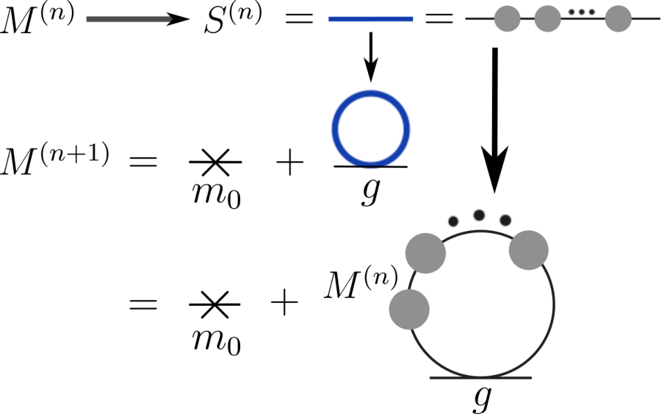
Now we set up the iterative method to sum up all tree diagrams. First of all, we classify diagrams in the tree according to the node length of each diagram. Node length of a diagram is defined by the maximum number of loops in a continuous route from the mass external line towards the edge loop, or maximum number of nodes of fat propagator legs in the diagram. Fig.2 shows the counting rule of node length and classification of diagrams.

Here we define $M^{(n)}$ as a sum of diagrams whose node length is no greater than $n$. Then we find the iteration transformation to evaluate $M^{(n+1)}$ by using $M^{(n)}$, which is shown in Fig.3. Note that the qualitative structure of this iteration transformation resembles much to that defined for the sum of geometric series (Appendix A). At every iteration, we make $n+1$ node diagram using $n$ node diagram by looping the corresponding propagator and finally add the $0$-node term $m_{0}$ which is not contained in the loop diagram.

The transformation function $F$,

$$M^{(n+1)}=F\left(M^{(n)}\right),$$

(6)

is given by the one loop integral as follows:

$$\begin{split}F(M)&=m_{0}+4\pi^{2}g\int\frac{d^{4}p}{(2\pi)^{4}}{\rm tr}\left[\frac{i}{{\vtop{\halign{#\cr\hfil/\hfil\crcr$p$\crcr}}}-M}\right]\\ &\hskip-20.0pt\scalebox{0.80}{$\xrightarrow{\text{Wick rotation}}$}~m_{0}+16\pi^{2}gM\int\frac{d^{4}p_{\rm E}}{(2\pi)^{4}}\frac{1}{{p_{\rm E}}^{2}+M^{2}}\\ &=m_{0}+16\pi^{2}gM\int d\Omega\int_{0}^{\Lambda}\frac{d|p_{\rm E}|}{(2\pi)^{4}}\frac{|p_{\rm E}|^{3}}{|p_{\rm E}|^{2}+M^{2}}\\ &=m_{0}+gM\left(1-M^{2}\log\left(1+M^{-2}\right)\right).\end{split}$$

(7)

Here all the variables are rescaled to be dimensionless taking the ultraviolet cutoff $\Lambda$ as the mass unit.

In conclusion, the total sum of the tree diagrams is obtained by $M^{(\infty)}$, that is, through infinitely many times of transformation by the same $F$.

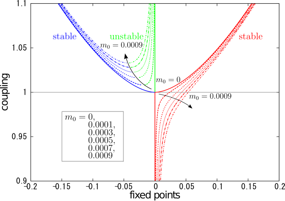
Iterative transformation here is best understood by a graphical method where the transformation function $y=F(x)$ and a straight line $y=x$ are drawn as shown in Fig.4. Each iteration process can be drawn on this figure by a successive moves of point. In any case the iterative transformation finally reaches a stable fixed point. Fixed points are crossing points between $y=F(x)$ and $y=x$, and position of fixed points are shown in Fig.5.

In the weak coupling region ($g=0.7$) shown in the upper diagram in Fig.4, there is only one fixed point near the origin and it is stable. The iteration should start with the initial condition $M^{(0)}=m_{0}$ and it approaches to the fixed point.

When the coupling constant becomes strong, there occurs pair creation of fixed points, one is stable and the other is unstable, which is seen in Fig.5 where move of fixed point positions are plotted for various $m_{0}$.

Then there are two stable fixed points each of which has its attractive region, territory. We must be careful about the initial starting point of iteration, $m_{0}$, that is, the essential question is in which territory does it start.

In all figures, we use positive $m_{0}$, then the initial point exists in the territory of the right-hand side stable fixed point, as seen in lower diagram in Fig.4. To prove this we investigate neighborhood of the origin, where the transformation function takes the following form,

$$F(x)\simeq m_{0}+kx,\ \ k>1.$$

(8)

Then the fixed point near the origin $x^{\star}_{0}$ is obtained as

$$x^{\star}\simeq m_{0}+kx^{\star}\longrightarrow x^{\star}\simeq\frac{m_{0}}{1-k},$$

(9)

that is, $x^{\star}_{0}$ is negative. Therefore, for all region of the coupling constant, the physical result is controlled by the right most stable fixed point in Fig.5.

Note that the critical coupling constant is defined for $m_{0}=0$. The criticality corresponds to the case that the gradient of iteration transformation function $F$ at the origin equals to unity. When it is larger than unity, there appears three fixed points and one at the origin becomes unstable. The gradient is quickly evaluated as

$$F^{\prime}(0)=g,$$

(10)

and therefore the critical coupling constant is obtained as

$$g_{\rm c}=1.$$

(11)

Let’s see some features of mass generation with respect to the node length $n$ in Fig.6. In the weak coupling case (upper diagram), the dynamical mass is generated rather quickly at low $n$ and becomes constant, which should be called the perturbative characteristics. By decreasing the bare mass the final mass goes to zero.

In the strong coupling case (lower diagram), the generation of the dynamical mass depends strongly on the bare mass, and it is mainly generated at some narrow range of node length. Decreasing the bare mass, the region of mass generating node length becomes large, but the output mass is almost constant, which means the spontaneous mass generation.

It is also seen that the shape of generation curves look the same form, just displacement in the node length space. These features are readily understandable by the iterative nature of our calculation well seen in the lower diagram in Fig.4. The move of iterated points is characterized from the unstable fixed point to the stable fixed point. When taking smaller bare mass, the starting point is nearer to the unstable fixed point and thus the growing up is delayed, thus larger node length region is important. The quick growing region is the mid of the two fixed points, and this assures the iteration behavior of mass growing is quite similar independent of $m_{0}$, just the translation in the node length space.

In Fig.7, we plot iterative development of mass as a function of $m_{0}$. The upper diagram is below critical and vanishing bare mass limit of $M$ is always vanishing.

The mid diagram is just on critical, and we see the appearance of infinite slope at the origin. The slope of $M$ with respect to $m_{0}$ is nothing but the susceptibility of the chiral condensate. Therefore, the susceptibility becomes divergent at $n\rightarrow\infty$, which is the characteristics of the 2nd order phase transition.

The lower diagram is super critical. Here vanishing bare mass limit of $M$ is vanishing also, for any finite $n$. This implies that for any finite node length $n$, the spontaneous mass generation does not occur. Of course, this is also well understandable if we imagine the iteration procedure in Fig.4. However, if we change the order of limit, that is, keeping the non-vanishing bare mass, we take the infinite node length limit first as

$$\lim_{m_{0}\rightarrow 0}[\lim_{n\rightarrow\infty}M^{(n)}(m_{0})],$$

(12)

then it gives a non-vanishing value. This should be regarded as the spontaneously generated mass.

In this way, we conclude the dynamical mass given by the iterative method as shown in Fig.8.

Here we comment on an implicit relation between unstableness of fixed point and the physicality condition. We rewrite the iteration transformation as

$\displaystyle M^{(n+1)}=F(M^{(n)})=m_{0}+F_{0}(M^{(n)})\ ,$

(13)

then fixed point $M^{\ast}$ satisfies

$\displaystyle M^{\ast}=F(M^{\ast})=m_{0}+F_{0}(M^{\ast})\ .$

(14)

The slope of function $F$ at a fixed point gives the eigenvalue of the transformation linearized around the fixed point and thus it determines the stability of it as shown in Fig.9.

The slope is calculated as

$\displaystyle\left.\frac{dF(M^{\ast})}{dM^{\ast}}\right|_{m_{0}\rm{fixed}}$

$\displaystyle=\frac{dF_{0}(M^{\ast})}{dM^{\ast}}=1-\frac{dm_{0}(M^{\ast})}{dM^{\ast}}.$

(15)

Therefore, the unstable fixed point,

$$F^{\prime}(M^{\ast})>1,$$

(16)

corresponds to the negative derivative,

$$\frac{dm_{0}(M^{\ast})}{dM^{\ast}}<0.$$

(17)

On the other hand in our model of NJL ladder, inverse of this derivative corresponds to the susceptibility $\chi$ of $\bar{\psi}\psi$ as

$$\frac{dM^{\ast}}{dm_{0}}=G\chi+1,$$

(18)

which is derived by Eq.(27). Then the unstable fixed point corresponds to the negative $\chi$, that is, negative fluctuation of $\bar{\psi}\psi$, which means the instability of the vacuum and absolutely unphysical solution. Inversely, the normal vacuum ($\chi>0$) assures the stability of fixed point $|F^{\prime}(x^{\ast})|<1$.

In this section, we calculate the free energy and the effective potential using the node length iteration. We define the free energy through the logarithm of the partition function as a function of the bare mass $m_{0}$:

$$W(m_{0})\equiv\ln Z(m_{0}),$$

(19)

where the partition function is given by

$$Z(m_{0})=\int{\mathcal{D}}\psi{\mathcal{D}}\bar{\psi}\exp\left(-\int d^{4}x_{\rm E}{\mathcal{L}}^{\rm E}_{\rm NJL}\right).$$

(20)

The free energy $W(m_{0})$ is the generating function of the connected Green function. Particularly its first derivative represents the vacuum expectation value of operator $\bar{\psi}\psi$ as follows:

	$\displaystyle\frac{\partial W(m_{0})}{\partial m_{0}}$	$\displaystyle=$	$\displaystyle\left<\int d^{4}x_{\rm E}\bar{\psi}(x_{\rm E})\psi(x_{\rm E})\right>_{m_{0}}=\int d^{4}x_{\rm E}\left<\bar{\psi}(0)\psi(0)\right>_{m_{0}}$		(21)
		$\displaystyle=$	$\displaystyle\Omega\left<\bar{\psi}\psi\right>_{m_{0}}\equiv\Phi,$

where $\left<\cdots\right>_{m_{0}}$ denotes the vacuum expectation value and due to the translational invariance of the vacuum there is no $x_{\rm E}$ dependence of $\left<\bar{\psi}\psi\right>_{m_{0}}$.

We introduce the Legendre transform of $W(m_{0})$ by defining $\Gamma(\Phi)$,

$$\Gamma(\Phi)\equiv-W(m_{0})+m_{0}\Phi\ .$$

(22)

Its derivative gives the bare mass in turn,

$$\frac{\partial\Gamma(\Phi)}{\partial\Phi}=-\frac{\partial m_{0}}{\partial\Phi}\frac{\partial W(m_{0})}{\partial m_{0}}+\frac{\partial m_{0}}{\partial\Phi}\Phi+m_{0}=m_{0}.$$

(23)

We move to the density of all these variables as follows:

$$w(m_{0})\equiv\frac{W(m_{0})}{N\Omega}\ ,\ \ \phi\equiv\frac{\Phi}{N\Omega}\ ,\ \ V_{\rm L}(\Phi)\equiv\frac{\Gamma(\Phi)}{N\Omega}\ ,\ \ \frac{\partial V_{\rm L}(\phi)}{\partial\phi}=m_{0}.$$

(24)

We also define the dimensionless variable $\tilde{\phi}$ by

	$\displaystyle\tilde{\phi}$	$\displaystyle\equiv$	$\displaystyle\frac{\phi}{\Lambda^{3}}=\frac{\Psi}{\Omega N\Lambda^{3}}$		(25)
		$\displaystyle=$	$\displaystyle\frac{1}{4\pi^{2}}{\tilde{M}}\left[1-{\tilde{M}}^{2}\ln\{1+{\tilde{M}}^{-2}\}\right].$		(26)

Hereafter we omit the tilde mark for the dimensionless variables and find the simple relation, $\phi$ as a function of $M$:

$$\phi=\frac{M-m_{0}}{G}.$$

(27)

Now we apply the node length iteration method to this relation and define node length iterated $\phi$, $w$ and $V_{\rm L}$ as follows:

$$\phi^{(n)}(m_{0})\equiv\frac{M^{(n)}-m_{0}}{G}\ ,\ \$$

(28)

$$\frac{\partial w^{(n)}(m_{0})}{\partial m_{0}}=\phi^{(n)}(m_{0})\ ,\ \ V^{(n)}_{\rm L}(\phi^{(n)})=-w^{(n)}(m_{0})+m_{0}\phi^{(n)}.$$

(29)

Using these relations, we first calculate $\phi^{(n)}$ as a function of $m_{0}$, and then integrate it to have the function $w^{(n)}(m_{0})$. Finally we obtain the Legendre effective potential function $V^{(n)}_{\rm L}$.

All these results are plotted in Fig.10 and Fig.11. Note that calculated Legendre effective potential are perfectly convex at any $n$, and therefore also convex at $n\rightarrow\infty$. To prove this property we recall the iteration transformation in Eq.(7),

$$M^{(n+1)}=F(M^{(n)})\ ,F(M)=m_{0}+gM(1-M^{2}\log(1+M^{-2})).$$

(30)

Differentiate both sides of this transformation with respect to $m_{0}$, we have

$$\frac{\partial M^{(n+1)}}{\partial m_{0}}=1+F^{\prime}(M^{(n)})\frac{\partial M^{(n)}}{\partial m_{0}}.$$

(31)

The derivative $F^{\prime}$ is found to be positive for the normal physical region $|M|\leq 0.7$. Taking account of the initial condition

$$\frac{\partial M^{(0)}}{\partial m_{0}}=1,$$

(32)

we get

$$\frac{\partial M^{(n)}}{\partial m_{0}}>1,$$

(33)

for any $n$. This inequality assures that at any $n$, the fluctuation of $\phi$ is always positive and hence the convexity of the Legendre effective potential.

These physically correct results are automatically obtained in our method of iterative evaluation of all physical variables. As is mentioned in the introduction, the iterative method here realizes something like the finite volume regularization.

In this section, we explore the finite density system. We add the chemical potential ($\mu$) term to the Nambu–Jona-Lasinio model Lagrangian as follows:

$${\mathcal{L}_{\rm NJL}}=\bar{\psi}i{{\vtop{\halign{#\cr\hfil/\hfil\crcr$\partial$\crcr}}}}\psi+\mu{\bar{\psi}}\gamma^{0}\psi-m_{0}{\bar{\psi}}\psi+\frac{G}{2N}\left[\left({\bar{\psi}\psi}\right)^{2}+\left(\bar{\psi}i\gamma_{5}\psi\right)^{2}\right].$$

(34)

Then the fermion propagator is changed as

$\displaystyle\frac{i}{{{\vtop{\halign{#\cr\hfil/\hfil\crcr$p$\crcr}}}}-m_{0}}\rightarrow\frac{i}{{{\vtop{\halign{#\cr\hfil/\hfil\crcr$p$\crcr}}}}+\mu\gamma^{0}-m_{0}},$

and the basic one-loop integral appearing in our iteration method now takes the following form:

$$\Sigma=4iG\int\frac{d^{4}p}{(2\pi)^{4}}\frac{M}{p^{2}+2\mu p^{0}+\mu^{2}-M^{2}}\ .$$

(40)

So far our model has an ultraviolet cutoff $\Lambda$ and we take the four-dimensional isotropic cutoff. Hereafter we take the so-called three-dimensional cutoff since it better fits to the case with finite temperature. The energy (time) component has no cutoff and only the momentum (space) components have the cutoff $\Lambda$, that is, the integration range for the energy and momentum takes the following ranges respectively,

$\displaystyle\left\{\begin{array}[]{l}p^{0}:-\infty\rightarrow\infty\ ,\\ |{\bm{p}}|:0\rightarrow\Lambda\ .\end{array}\right.$

Transforming to the Euclidean coordinate, we have

$$\Sigma=\frac{4GM}{(2\pi)^{4}}\int_{0}^{\Lambda}d^{3}p\int_{-\infty}^{\infty}dp^{4}\frac{1}{\{p^{4}-i(\mu+\omega_{\bm{p}})\}\{p^{4}-i(\mu-\omega_{\bm{p}})\}}\ ,$$

(44)

where $\omega_{\bm{p}}\equiv\sqrt{{\bm{p}}^{2}+M^{2}}$. We integrate the time component by using the residue theorem to have

$$\Sigma=\frac{GM}{\pi^{2}}\int_{0}^{\Lambda}dp\ \theta(\sqrt{p^{2}+M^{2}}-\mu)\frac{p^{2}}{\sqrt{p^{2}+M^{2}}}\ .$$

(45)

Finally, we obtain the loop integral:

	$\displaystyle\Sigma$	$\displaystyle=2gM\theta(\sqrt{1+M^{2}}-\mu)\left[\theta(|M|-\mu)\left\{\sqrt{1+M^{2}}+M^{2}\ln\frac{|M|}{1+\sqrt{1+M^{2}}}\right\}\right.$
		$\displaystyle{}\left.+\theta(\mu-|M|)\left\{\sqrt{1+M^{2}}-\mu\sqrt{\mu^{2}-M^{2}}+M^{2}\ln\frac{\mu+\sqrt{\mu^{2}-M^{2}}}{1+\sqrt{1+M^{2}}}\right\}\right],$		(46)

where all variables are rescaled to be dimensionless with unit $\Lambda$ and we use the rescaled coupling constant $g=G/(2\pi^{2})$. Note that in our three-dimensional cutoff the critical coupling constant (for $\mu=0$) is $2\pi^{2}$, just a half of that of the four-dimensional cutoff. This change of the physical criticality comes from the fact that the NJL model is not a renormalizable theory and the cutoff scheme is a part of definition of the theory.

We set up the node length iteration using the above cutoffed integral $\Sigma$ as follows:

$\displaystyle M^{(n+1)}=F(M^{(n)})=m_{0}+\Sigma(M^{(n)})$

(47)

The iteration function $F(M)$ can have five fixed points at most in case of strong coupling and low chemical potential. We plot an example of the iteration function in Fig.12 where five crossing points are observed.

The total structure of the fixed point map is drawn in Fig.13 for fixed $g=0.85$ and in Fig.14 for fixed $\mu=0.7$. These figures clearly show that we encounter the 1st order phase transition. In Fig.13, looking down in the direction of the chemical potential from 1, or in Fig.14, looking up in the direction of $g$ from 0, at some point there appears pair creation of fixed points far from the origin, one is stable and the other is unstable, while the origin still survives as a stable fixed point. This region with five fixed points correspond to the triple-well image of the potential.

We investigate the node length iteration of $M{(n)}$ and $\phi^{(n)}$ for $g=0.85,\mu=0.7$ in Fig.15. For large enough bare mass $m_{0}$, the dynamical mass $M$ and $\phi$ are generated. However, if we take the vanishing bare mass limit we have vanishing $M$ and $\phi$. Then the Legendre effective potential calculated by iteration method takes the form depicted in Fig.16 where we may see the chiral symmetry broken points at $\phi\simeq 0.013$, but the minimum of the effective potential is still at the origin. Note that the convexity of the Legendre effective potential is automatically assured as before.

Referring to another type of analysis of this system, we understand that the model with parameter $g=0.85,\mu=0.7$ resides in the chiral symmetry broken phase, that is, the dynamical mass is generated spontaneously. Considering this situation, the node length iteration formulated so far does not always give correct vacuum for 1st order phase transition case. In other words, as far as the origin stands for the stable fixed point, the vanishing bare mass limit of iteration always goes into the origin.

Here we prove this property by comparing our results with those obtained in Kuma14-1 by using the weak solution method of the non-perturbative renormalization group analysis of the dynamical chiral symmetry breaking. In Fig.17, we plot the mass as a function of $m_{0}$ for various $\mu$ with $g=0.85$.

There are 4 plots in each figure. The dashed line is a multi-valued function of $m_{0}$ which is obtained from the Schwinger-Dyson equation, or the position of all fixed points in our iteration method. The straight line is $M=m_{0}$ and shows the initial condition for the iteration method. Starting with this line $M=m_{0}$, we readily obtain the infinite $n$ limit of iteration, which is the red curve, just as drawn in Fig.15.

The thin blue curve is the weak solution defined in Kuma14-1. The weak solution determines the unique function by a patchwork of the multi-valued function so that the vertical jump line gives the equal area for left and right sides of the jump. Note that in figure (b), the 4 parts are balanced totally. This balance of the area assures that the resultant Legendre effective potential is properly convexified and therefore the obtained mass $M(m_{0})$ is always physically correct.

Therefore, in the parameter regions where the red curve is different from the blue curve, the iteration method does not give the physically correct mass. In figure (a) there is no such region. This is the same type of multi-valuedness as zero density case, that is the double well type transition.

In figures (b), (c), (d), the iteration goes wrong at some $m_{0}$ intervals. The mismatch is the $m_{0}$ value where the finite jump occurs between two stable fixed points. The blue line separates the multi-valued region into equal area parts, while the red line always passes the extremum point.

In figure (b), even the vanishing $m_{0}$ limit is wrong, Note that in cases (c) and (d), although the vanishing $m_{0}$ limit is correct, the difference remain for large $m_{0}$ region which is also physical region anyway.

We concentrate on case (b). There is a stable fixed point around the origin and iteration goes to this fixed point. It is impossible to give the physically correct result (blue line) since this stable fixed point is above the initial condition line $M=m_{0}$ in the positive $m_{0}$ region near the origin. To prove this property, we expand the transformation function $F(x)$ around the origin,

$$F(x)\simeq m_{0}+kx,$$

(48)

where the stability of the fixed point indicates $k<1$. Then the fixed point $x^{\star}_{0}$,

$$x^{\star}_{0}\simeq\frac{m_{0}}{1-k},$$

(49)

is larger than $m_{0}$. Therefore the iteration starting with $m_{0}$ resides in the attractive domain of this stable fixed point near the origin, although this stable fixed point is actually a meta-stable state and cannot be the physical vacuum.

This failure of our iteration method in case of 1st order phase transition must be reconsidered here from a different view point, since it is related to issue of multi-valuedness of the infinite sum of Feynman diagrams even within our method of iteration transformation. In fact, we use the propagator where the mass is inserted in the denominator, which means we have done some partial but infinite sum of geometric series first in a particular manner.

Suppose we set up another shifted iteration system where we add fictitious bare mass $M_{0}$ to the propagator and subtract the same quantity in the interaction part. We define the node length counting so that the four-fermi interactions and the negative counter mass interaction play the equal level role. The infinite iteration apparently gives the sum of all $1/N$ leading diagrams.

This shifted iteration, however, corresponds exactly to the original iteration starting with a different initial point of $M_{0}+m_{0}$. Then by choosing the fictitious bare mass $M_{0}$ appropriately, we may select any fixed point of iteration as the infinite iteration result. This shows that our iteration method cannot completely avoid the total indefiniteness of the infinite sum of $1/N$ leading diagrams.

In this section, we investigate the dynamical chiral symmetry breaking in gauge theories. We consider the so-called ladder or planar approximation for the fermion self-energy. The ladder type diagram means that all the gluons are not crossed to each other. For the total sum of those ladder type diagrams we can find the whole as a part and set up the self-consistent condition which is drawn as in Fig.18, where the straight line represents a fermion and circular lines represent gluons. This is an integral equation and there are infinite number of non-trivial solutions for strong enough gauge coupling constant.

To set up an iterative method to sum up all ladder diagrams, we first define the ladder depth for each planar diagram. The ladder depth is the maximum number of gluon propagators counting from the most outer loop towards the fermion propagator. For example we show a diagram with ladder depth = 5 in Fig.19.

Then we define mass function $\Sigma^{(n)}$ which contains all planar diagrams whose ladder depth is no greater than $n$. Now we set up the iteration transformation as shown in Fig.20.

The iteration functional is denoted by

$\displaystyle{\Sigma}^{(n+1)}(x)$

$\displaystyle=$

$\displaystyle\mathscr{F}\left[{\Sigma}^{(n)}(x)\right],$

(50)

where argument $x$ is the Euclidean momentum squared. The functional is calculated by one loop integral of the Feynman diagram as followsaoki:

	$\displaystyle\mathscr{F}[{\Sigma(x)}]\kern-11.38109pt$	$\displaystyle=$	$\displaystyle\kern-14.22636ptm_{0}+\int^{\Lambda}\frac{d^{4}p}{i(2\pi)^{4}}C_{2}(R)\left(\theta(p^{2}-k^{2})g^{2}(p^{2})+\theta(k^{2}-p^{2})g^{2}(k^{2})\right)$		(54)
		$\displaystyle\quad\times$	$\displaystyle\frac{g^{\mu\nu}-(p-k)^{\nu}/(p-k)^{2}}{(p-k)^{2}}\gamma_{\mu}\frac{1}{{\vtop{\halign{#\cr\hfil/\hfil\crcr$k$\crcr}}}-\Sigma(k)}\gamma_{\nu}$
		$\displaystyle=$	$\displaystyle\kern-14.22636ptm_{0}+\frac{3C_{2}(R)}{16\pi^{2}}\int^{\Lambda^{2}}_{0}dy\frac{y\Sigma(y)}{y+\Sigma^{2}}\left(\frac{g^{2}(x)}{x}\theta(x-y)+\frac{g^{2}(y)}{y}\theta(y-x)\right)$
		$\displaystyle=$	$\displaystyle\kern-14.22636ptm_{0}+\frac{\lambda(x)}{4x}\int_{0}^{x}\frac{y\Sigma(y)dy}{y+\Sigma^{2}(y)}+\int_{x}^{\Lambda^{2}}\frac{\lambda(y)\Sigma(y)dy}{4(y+\Sigma^{2}(y))},$

where we set $x=p^{2},y=k^{2}$ and $\lambda$ is defined by the running gauge coupling constant $g(x)$,

$$\lambda(x)=\frac{3g^{2}(x)}{4\pi^{2}},$$

(55)

and $C_{2}(R)$ is the second Casimir invariant for the fermion representation $R$.

Note that the mass function $\Sigma(x)$ is a function of momentum squared $x$. The functional $\mathscr{F}$ is now an infinite dimensional map and there are infinite number of fixed point functions. Our analysis clarified that only one of fixed point functions is perfectly stable and is reached by proper initial function $\Sigma^{(0)}(x)=m_{0}$.

Hereafter numerical calculations are performed for U(1) gauge theory with fixed gauge coupling constant where $\lambda_{\rm c}=1$. However, all the results are expected to hold qualitatively for the QCD with running gauge coupling constant.

Starting with the initial constant function, $\Sigma^{(n)}(p)$ develops according to the ladder depth iteration as shown in Fig.21. The dynamical mass is given by $\Sigma^{(n)}(0)$, and its iterative development is plotted in Fig,22 for $\lambda=0.9$ (left) and $\lambda=1.5$ (right), where the left most plot point corresponds to the bare mass $m_{0}$. We decrease $m_{0}$ in order ($0.01,0.001,0.0001$), and check the response of $\Sigma^{(n)}(0)$. We can see the switch-on of the spontaneous mass generation for the strong enough gauge coupling constant in Fig.22 (right).

We check the fixed point of this iterative transformation for the super critical ($\lambda>1$) case. We omit the detailed argument hereSD. All fixed points are ordered with respect to the number of nodes in the fixed point function $\Sigma(x)$. We investigate first three fixed point functions (number of nodes = 0, 1, 2) and calculate eigenvalues around them. We plot eigenvalues in Fig.23. Eigenvalues less than unity corresponds to attractive direction whereas those larger than unity means repulsive direction.

As for the 1st fixed point, all eigenvalues are less than unity and it is a completely attractive fixed point. Therefore starting from the initial function $\Sigma^{(0)}=m_{0}$, we have a convergent result towards this fixed point function for infinite number of iterations. For the 2nd fixed point there appear one eigenvalue larger than unity and it is unstable for this direction. In fact, this direction is nothing but a route to the 1st fixed point in our function space. The 3rd fixed point has two eigenvalues larger than unity. This type of breakup series of fixed points is a very standard image of the spontaneous symmetry breaking in function space. It is pictured in Fig.24 where all fixed points are drawn pair-wisely due to the original chiral symmetry (precisely speaking it is U(1) rotational symmetry).

We have proposed a new method of calculating the spontaneous mass generation for the dynamical chiral symmetry breaking. We work with Nambu–Jona-Lasinio model and gauge theories. We define the node length classification for NJL mode, and the ladder depth classification for gauge theories.

The iteration method can directly evaluate the mass without any singularity and automatically reaches the physically correct solution. However for the finite density system, where 1st order phase transition occurs, the iteration method gives a physically inappropriate solution in case that symmetric vacuum remains meta-stable state. This miss-match, however, implies a deeper problem in evaluating infinite sum of Feynman diagrams and give us a subject to be attacked.

We thank illuminating discussions with Yasuhiro Fujii and Masatoshi Yamada. This work was partially supported by JSPS KAKENHI Grant Number 16K13848 and the 2016 Research Grant of Yonago National College of Technology.

References

- (1) K-I. Aoki, Int. J. Mod. Phys. B 14 (2000) 1249–1326.
- (2) Y. Nambu and G. Jona-Lasinio, Phys. Rev. 122, 345 (1961); 124, 246 (1961).
- (3) K-I. Aoki, S-I. Kumamoto and D. Sato, Prog. Theor. Exp. Phys., 2014, 043B05 (2014).
- (4)
K. Higashijima, Phys.Rev. D29 (1984) 1228.
K-I. Aoki, M. Bando, T. Kugo, M.G. Mitchard and H. Nakatani, Prog. Theor. Phys. 84, 683 (1990). - (5)
T. Maskawa and H. Nakajima, Prog. Theor. Phys. 52 (1974), 1326.
R. Fukuda and T. Kugo, Nucl. Phys. B117 (1976), 250.