Identification, Secrecy, Template, and Privacy-Leakage of Biometric Identification System Under Noisy Enrollment

Calligraphic $\mathcal{A}$ stands for a finite alphabet. Upper-case $A$ denotes a RV taking values in $\mathcal{A}$ and lower-case $a\in\mathcal{A}$ denotes its realization. $P_{A}(a)~\mathrel{\mathop{:}}=~\Pr[A=a]$, $a\in\mathcal{A}$, represents the probability distribution on $\mathcal{A}$, and $P_{A^{n}}$ represents the probability distribution of RV $A^{n}=(A_{1},\cdots,A_{n})$ in $\mathcal{A}^{n}$, the $n$th Cartesian product of $\mathcal{A}$. $P_{A^{n}B^{n}}$ represents the joint probability distribution of a pair of RVs $(A^{n},B^{n})$ and its conditional probability distribution $P_{A^{n}|B^{n}}$ is defined as

The entropy of RV $A$ is denoted by $H(A)$, the joint entropy of RVs $A$ and $B$ is denoted by $H(A,B)$, and the mutual information between $A$ and $B$ is denoted by $I(A;B)$ [10]. Throughout this paper, logarithms are of base two. For integers $a$ and $b$ such that $a\leq b$, $[a,b]$ denotes the set $\{a,a+1,\cdots,b\}$. A partial sequence of a sequence $c^{n}$ from the first symbol to the $t$th symbol $(c_{1},\cdots,c_{t})$ is represented by $c^{t}$.

Here, we define the strong typicality property and use the same notation as in [10]. A sequence $x^{n}\in\mathcal{X}^{n}$ is said to be $\delta$-$strongly~typical$ with respect to a distribution $P_{X}$ on $\mathcal{X}$ if $|\frac{1}{n}N(a|x^{n})-P_{X}(a)|\leq\delta$ and $P_{X}(a)=0$ implies $\frac{1}{n}N(a|x^{n})=0$ for all $a\in\mathcal{X}$, where $N(a|x^{n})$ is the number of occurrences of $a$ in the sequence $x^{n}$, and $\delta$ is an arbitrary positive number. The set of sequences $x^{n}\in\mathcal{X}^{n}$ such that $x^{n}$ is $\delta$-strongly typical is called the strongly typical set and is denoted by $A^{(n)}_{\epsilon}(X)$. This concept is easily extended to joint distributions.

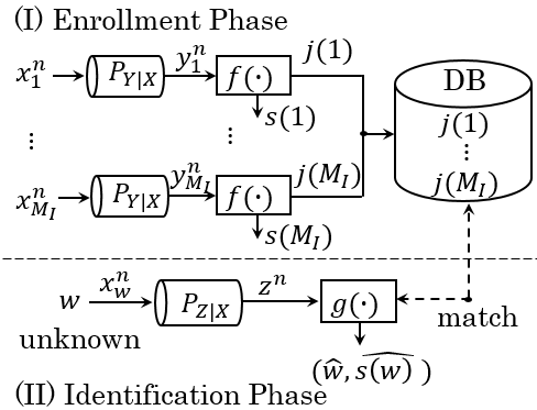
The BIS model studied in this paper is shown in Fig. 1. It consists of two phases: (I) Enrollment Phase, and (II) Identification Phase. Next, we will explain the details of each phase.

Let $\mathcal{I}=[1,M_{I}]$ and $\mathcal{X}$ be the sets of indexes of individuals and a finite source alphabet, respectively. For any $i\in\mathcal{I}$, we assume that $x^{n}_{i}=(x_{i1},\cdots,x_{in})\in\mathcal{X}^{n}$, an $n$-length bio-data sequence of individual $i$, is generated i.i.d. from a stationary memoryless source $P_{X}$. The generating probability for each sequence $x^{n}_{i}\in\mathcal{X}^{n}$ is

Now let $\mathcal{J}=[1,M_{J}]$ and $\mathcal{S}=[1,M_{S}]$ be the sets of indexes of templates stored in database and individuals’ secret data, respectively. All bio-data sequences are observed via a stationary DMC $\{\mathcal{Y},P_{Y|X},\mathcal{X}\}$, where $\mathcal{Y}$ is a finite output-alphabet of $P_{Y|X}$. The corresponding probability that $x^{n}_{i}\in\mathcal{X}^{n}$ is observed as $y^{n}_{i}=(y_{i1},y_{i2},\cdots,y_{in})\in\mathcal{Y}^{n}$ via the DMC $P_{Y|X}$ is

Bio-data sequence $x_{w}^{n}\ (w\in\mathcal{I})$ of an unknown $w$ (index of individual enrolled in the database) is observed via a DMC $\{\mathcal{Z},P_{Z|X},\mathcal{X}\}$, where $\mathcal{Z}$ is a finite output-alphabet of $P_{Z|X}$. The corresponding probability that $x^{n}_{w}\in\mathcal{X}^{n}$ is output as $z^{n}=(z_{1},z_{2},\cdots,z_{n})\in\mathcal{Z}^{n}$ via $P_{Z|X}$ is given by

The decoder observers the identified sequence $Z^{n}$ and estimates the pair of index and secret data by comparing $Z^{n}$ with all templates $\mathcal{J}_{M_{I}}$ in the database $(\widehat{W},\widehat{S(W)})=g(Z^{n},\mathcal{J}_{M_{I}})$, where $g$ denotes decoding function.

The motivation to analyze performance of the BIS provided that the distribution of $I$ is unknown is that the identified frequencies of each individual are likely different. For example, it is hard to think that the frequencies of coming to use a bank teller of each individual are identical. For real applications, this assumption is important to take care of.

First, we fix $\delta>0$ arbitrarily small, and a block length $n$. We also fix test channels $P_{U|Y}$ and $P_{V|U}$. We set^*1*1 *1 Due to the Markov chain $V-U-Z$, we have $I(Z;U)-I(Z;V)=I(Z;UV)-I(Z;V)=I(Z;V)+I(Z;U|V)-I(Z;V)=I(Z;U|V)$. In the proof, we use this fact without explanation. $R_{I}=I(Z;V)-\delta$, $R_{S}=I(Z;U|V)-\delta$, $R_{J}=I(Y;U)-I(Z;U)+I(Z;V)+3\delta$, and $R_{L}=I(X;U)-I(Z;U)+I(Z;V)+3\delta$. We also set $M_{I}=2^{nR_{I}}$, $M_{S}=2^{nR_{S}}$, and $M_{J}=2^{nR_{J}}$, respectively.

Sequences $v^{n}_{m}$ are generated i.i.d. from $P_{V}$ for $m~{\in}~[1,N_{V}]$, where $N_{V}=2^{n\left(I(Y;V)+\delta\right)}$. For each $m$, sequences $u^{n}_{k|m}$ are generated from the memoryless channel $P_{U^{n}|V^{n}=v_{m}^{n}}$ for $k~{\in}~[1,N_{U}]$, where $N_{U}=2^{n\left(I(Y;U|V)+\delta\right)}$. Divide these sequences equally from the first index into $N_{B}={2^{n\left(I(Y;U|V)-I(Z;U|V)+2\delta\right)}}$ bins. That is, the first bin contains $\{u^{n}_{1|m},\cdots,u^{n}_{M_{S}|m}\}$, the second bin contains $\{u^{n}_{M_{S}+1|m},\cdots,u^{n}_{2M_{S}|m}\}$, and so on. Consequently, each bin contains exactly $M_{S}$ codewords. Bins are indexed by $b\in[1,N_{B}]$ and codewords inside a certain bin are indexed by $s\in\mathcal{S}$. Without loss of generality, there exists a one-to-one mapping between $k$ and the pair $(b,s)$.

When encoder $f$ observes the bio-data sequence $y^{n}_{i}$, the encoder looks for $(m,k)$ such that $(y^{n}_{i},v^{n}_{m},u^{n}_{k|m})\in A_{\epsilon}^{(n)}(YVU)$. In case there are more than one such pairs, the encoder picks one of them uniformly at random. Assume that the encoder found a corresponding pair $(m,k)=(m(i),k(i))$ satisfying the jointly typical condition above. We set the template $j(i)=(m(i),b(i))$ and the secret data to be the corresponding codeword’s index $s(i)$ in bin $b(i)$ ^*2*2 *2 Since there is a one-to-one mapping between $k$ and $(b,s)$, we identify $k(i)$ with $(b(i),s(i))$.. $j(i)$ is stored at position $i$ in the database and $s(i)$ is handed back to individual $i$. If there do not exist such $m$ and $k$, then we set $j(i)={(1,1)}$ and $s(i)=1$.

The decoder has access to all records in the database $\{(m(1),b(1)),\cdots(m(M_{I}),b(M_{I}))\}$. When decoder $g$ sees $z^{n}$, the noisy version of identified individual sequence $x^{n}_{w}$, it checks whether the codeword pair $(v^{n}_{m(i)},u^{n}_{b(i),s|m(i)})$ is jointly typical with $z^{n}$ or not for all $i\in\mathcal{I}$ with some $s\in\mathcal{S}$, i.e. $(z^{n},v^{n}_{m(i)},u^{n}_{b(i),s|m(i)})\in A_{\epsilon}^{(n)}(ZVU)$. If there exists a unique pair ${(i,s)}$ for which this condition holds, then the decoder outputs $(\widehat{w},\widehat{s(w)})={(i,s)}$ as the estimated index and secret data, respectively. Otherwise, the decoder outputs the index of the template $(1,1)$ as $\hat{w}$ and $\widehat{s(w)}=1$ if (i) there does not exist such a pair $(i,s)$, (ii) such a pair $(i,s)$ exists but there are some $s^{\prime}\neq{s}$ ($s^{\prime}\in\mathcal{S}$) such that $(z^{n},v^{n}_{{m(i)}},u^{n}_{{b(i)},s^{\prime}|{m(i)}})\in A_{\epsilon}^{(n)}(ZVU)$ satisfies, or (iii) such a pair $(i,s)$ exists but there are some $i^{\prime}\neq{i}$ such that the pair $(v^{n}_{m(i^{\prime})},u^{n}_{b(i^{\prime}),{s^{\prime}}|m(i^{\prime})})$ is jointly typical with $z^{n}$ for some $s^{\prime}\in\mathcal{S}$.

We evaluate the ensemble average of the error probability, where the average is taken over randomly chosen codebook $\mathcal{C}_{n}$, which is defined as the set $\{V_{m}^{n},U_{k|m}^{n}:m\in[1,N_{V}],k\in[1,N_{U}]\}$. Let the pair $(M(i),K(i))=(M(i),B(i),S(i))$ denote the RVs corresponding to the index pair $(m(i),k(i))=(m(i),b(i),s(i))$ of sequences $V_{m}^{n}$ and $U_{k|m}^{n}$ determined by the encoder for $Y^{n}_{i}$. For individual $W=w$, possible event of errors occurs at the encoder is:

1. $\mathcal{E}_{1}$:  {$(Y^{n}_{w},V^{n}_{m},U^{n}_{k|m})\notin A_{\epsilon}^{(n)}(YVU)$
       for all $m\in[1,N_{V}]$ and $k\in[1,N_{U}]$},

   and those at the decoder are:

2. ${\mathcal{E}_{2}}$:  {$(Z^{n},V^{n}_{M(w)},U^{n}_{B(w),S(w)|M(w)})\notin A_{\epsilon}^{(n)}(ZVU)$},

3. ${\mathcal{E}_{3}}$:  {$\exists s^{\prime}\neq S(w)$ s. t.
       $(Z^{n},V^{n}_{M(w)},U^{n}_{B(w),s^{\prime}|M(w)})\in A_{\epsilon}^{(n)}(ZVU)$},

4. ${\mathcal{E}_{4}}$:  {$\exists i^{\prime}\neq w$ and $\exists s^{\prime}$ s. t.
       $(Z^{n},V^{n}_{M(i^{\prime})},U^{n}_{B(i^{\prime}),s^{\prime}|M(i^{\prime})})\in A_{\epsilon}^{(n)}(ZVU)$}.

Then, the error probability for $W=w$ can be bounded as

where (a) follows because $\Pr\left\{\mathcal{E}_{1},\mathcal{E}_{2}\right\}=\Pr\left\{\mathcal{E}_{1}\right\}+\Pr\left\{\mathcal{E}_{2}\cap\mathcal{E}^{c}_{1}\right\}\leq\Pr\left\{\mathcal{E}_{1}\right\}+\Pr\left\{\mathcal{E}_{2}|\mathcal{E}^{c}_{1}\right\}$.

$\Pr\{\mathcal{E}_{1}\}$ can be made smaller than $\delta$ for large enough $n$ by utilizing the covering lemma [12, Lemma 3.3] because $\frac{1}{n}\log N_{V}=I(Y;V)+\delta~{>I(Y;V)}$ and $\frac{1}{n}\log N_{U}=I(Y;U|V)+\delta~{>I(Y;U|V)}$. For $\Pr\left\{{\mathcal{E}_{2}|\mathcal{E}^{c}_{1}}\right\}$, it can also be made smaller than $\delta$ by the Markov lemma [10, Lemma 15.8.1]. By applying the packing lemma [12, Lemma 3.1], $\Pr\left\{{\mathcal{E}_{3}}\right\}$ and $\Pr\left\{{\mathcal{E}_{4}}\right\}$ are arbitrarily small for large enough $n$ since ${\frac{1}{n}\log M_{S}=I(Z;U|V)-\delta<I(Z;U|V)}$ and ${\frac{1}{n}\log M_{I}+\frac{1}{n}\log M_{S}=I(Z;U)-2\delta<I(Z;UV)}$, respectively.

Therefore, the ensemble average of the error probability can be made that

for large enough $n$.

We consider a virtual system, where a partial decoder $g_{i}$ is employed, for deriving the upper bound on the privacy-leakage rate. In this system, knowing index $i$ and seeing $Z^{n}_{i}$ (defined as the output sequence of $X^{n}_{i}$ via $P_{Z|X}$), the partial decoder $g_{i}$ estimates only the secret data of individual $i$ as $\widehat{S(i)}=g_{i}(Z^{n}_{i},J(i))$. Note that this system is just for analysis, and the partial decoder is not actually used during the decoding process.

For any given $i\in\mathcal{I}$, the partial decoder $g_{i}$ operates as follows: observing $z_{i}^{n}$ and the template $j(i)=(m(i),b(i))$ in the database, it looks for $s\in\mathcal{S}$ such that $(z^{n}_{i},v^{n}_{m(i)},u^{n}_{b(i),s|m(i)})\in A_{\epsilon}^{(n)}(ZVU)$. It sets $\widehat{s(i)}=s$ if there exists a unique $s$. Otherwise, it outputs $\widehat{s(i)}=1$. The potential events of error probability for this case are ${\mathcal{E}_{2}}$ and ${\mathcal{E}_{3}}$. Letting $P_{e}(i)$ be the error probability of $g_{i}$, we readily see that

where the middle term in (18) denotes the error probability of $g$ (in the original BIS) for individual $W=i$.

The function of this partial decoder enables us to bound the following conditional entropy

where

1. (b)

   follows because conditioning reduces entropy,

2. (c)

   follows because Fano’s inequality and (18) are applied, and ${\delta_{n}}=\frac{1}{n}\left(1+4\delta\log M_{S}\right)$.

Due to the fact that we set $M_{S}=2^{nR_{S}}$ and $M_{J}=2^{nR_{J}}$, the following inequalities hold

with equality when $S(i)$ and $J(i)$ are uniformly distributed on $\mathcal{S}$ and $\mathcal{J}$, respectively, for any codebook $\mathcal{C}_{n}$.

Hereafter, we shall check the bounds of identification, secrecy, secrecy-leakage, template, and privacy-leakage rates averaged over randomly chosen codebook $\mathcal{C}_{n}$. In the following analyses, the index $i$ is arbitrarily fixed on $\mathcal{I}$ since we need to show that all conditions in Definition 1 are satisfied.

From the parameter settings of achievability scheme, it is straight-forward that the conditions (7) and (9) hold.

The secrecy rate can be evaluated as follows:

where

1. (d)

   holds because $(J(i),S(i))$ is a function of $Y^{n}_{i}$,

2. (e)

   follows because (24) and Lemma 2 are applied,

3. (f)

   holds because we set $R_{S}=I(Z;U)-I(Z;V)-\delta$.

The amount of leaked information about $S(i)$ from $J(i)$ can be expanded as

where (g) follows because (23), (24), and Lemma 2 are applied.

In view of (11), we start by expanding the privacy-leakage rate $\frac{1}{n}I(X^{n}_{i};J(i)|\mathcal{C}_{n})$ as

where the inequality in (27) holds due to (24). Next, let us focus solely on the conditional entropy in (27). It can be evaluated as

References

• [1] J. A. O’Sullivan and N. A. Schmid, “Large deviations performance analysis for biometrics recognition,” in Proc. 40th Annual Allerton Conf. on Communication, Control, and Computing, pp. 1–19, Allerton House, IL, USA, Oct. 2002.
• [2] F. Willems, T. Kalker, S. Baggen, and J. P. Linnartz, “On the capacity of a biometric identification system,” in Proc. IEEE Int. Symp. Inf. Theory, Yokohama, Japan, p.82, Jun./Jul. 2003.
• [3] E. Tuncel, “Capacity/Storage tradeoff in high-dimensional identification systems,”, IEEE Trans. Inf. Theory, vol. 55, no. 5, pp. 2097–2016, May 2009.
• [4] T. Ignatenko and F. Willems, “Fundamental limits for privacy-preserving biometric identification system that support authentication,” IEEE Trans. Inf. Theory, vol. 61, no. 10, pp.5583–5594, Oct. 2015.
• [5] T. Ignatenko and F. Willems, “Biometric systems: Privacy and secrecy aspects,” IEEE Trans. Inf. Forensics Security, vol. 4, no. 4, pp.956–973, Dec. 2009.
• [6] O. Günlü and G. Kramer, “Privacy, secrecy, and storage with multiple noisy measurements of identifiers,” IEEE Trans. Inf. Forensics Security, vol. 13, no. 11, pp. 2872–2883, Nov. 2018.
• [7] M. Koide and H. Yamamoto, “Coding theorems for biometric systems,” in Proc. IEEE Int. Symp. Inf. Theory, Texas, USA, pp. 2647–2651, Jun. 2010.
• [8] V. Yachongka and H. Yagi, “Fundamental trade-off among identification, secrecy and template rates in identification system,” in Proc. 2018 Int. Symp. on Inf. Theory and Its Appl., p. 507 Singapore, Oct. 2018.
• [9] V. Yachongka and H. Yagi, “Fundamental tradeoff among identification, secrecy and compression rates in biometric identification system,” Journal of Signal Processing, vol. 22, no. 6, pp.337–342, Nov. 2018.
• [10] T. M. Cover and J. A. Thomas,  Elements of Information Theory, 2nd ed., John Wiley & Sons, New Jersy, 2006.
• [11] K. Kittichokechai and G. Caire, “Secret key-based identification and authentication with a privacy constraint,” IEEE Trans. Inf. Theory, vol. 62, no. 11, pp. 6189–6203, Nov. 2016.
• [12] A. El Gamal and Y.-H. Kim,  Network Information Theory, Cambridge, U.K.: Cambridge Univ. Press, 2011.
• [13] K. Kittichokechai, T. J. Oechtering, M. Skoglund, and Y.-K. Chia, “Secure source coding with action-dependent side information,” IEEE Trans. Inf. Theory, vol. 61, no. 12, pp. 6444–6464, Dec. 2015.
• [14] M. Bloch and J. Barros,  Physical-Layer Security, Cambridge, U.K.: Cambridge Univ. Press, 2011.
Appendix A Proof of Equation (15)
In the proof, we show the equivalence of 𝒜1\mathcal{A}_{1} and 𝒜2\mathcal{A}_{2} by removing the cardinality bounds of auxiliary RVs UU and VV from the two regions. Once the equivalence without the cardinality bounds is established, the cardinality bounds follow from the standard arguments (cf. [12, Appendix C]).
It is obvious that 𝒜2⊆𝒜1\mathcal{A}_{2}\subseteq\mathcal{A}_{1}, so we shall show that 𝒜2⊇𝒜1\mathcal{A}_{2}\supseteq\mathcal{A}_{1}. We assume that (RI,RS,RJ,RL)∈𝒜1(R_{I},R_{S},R_{J},R_{L})\in\mathcal{A}_{1}, meaning that (RI,RS,RJ,RL)(R_{I},R_{S},R_{J},R_{L}) satisfies all conditions in (13) for some PU|YP_{U|Y}. Especially, we have RI+RS≤I⁡(Z,U)R_{I}+R_{S}\leq I(Z;U). We choose the test channel PV|UP_{V|U} satisfying that
RI=I⁡(Z,V).\displaystyle R_{I}=I(Z;V). (53)
Such PV|UP_{V|U} always exists since I⁡(Z,U)≥I⁡(Z,V)≥0I(Z;U)\geq I(Z;V)\geq 0 and I⁡(Z,V)I(Z;V) is a continuous function of PV|UP_{V|U}. Under that condition, it is easy to check that (RI,RS,RJ,RL)(R_{I},R_{S},R_{J},R_{L}) is also an element lying in the region 𝒜2\mathcal{A}_{2}. ∎
Appendix B Proof of Lemma 2
In [4], a similar result of this lemma is used without the proof. Here, we will provide a proof for readers’ sake.
Note that J⁡(i)=(M⁡(i),B⁡(i))J(i)=(M(i),B(i)). We start by considering the conditional entropy in the left-hand side of (22) as
1n​H​(Yin|J⁡(i),S⁡(i),𝒞n)\displaystyle\textstyle\frac{1}{n}H(Y^{n}_{i}|J(i),S(i),\mathcal{C}_{n}) =1n​H​(Yin|M⁡(i),B⁡(i),S⁡(i),𝒞n)\displaystyle=\textstyle\frac{1}{n}H(Y^{n}_{i}|M(i),B(i),S(i),\mathcal{C}_{n})
=(a)​1n​H​(Yin|M⁡(i),B⁡(i),S⁡(i),Uin,𝒞n)\displaystyle\overset{\mathrm{(a)}}{=}\textstyle\frac{1}{n}H(Y^{n}_{i}|M(i),B(i),S(i),U^{n}_{i},\mathcal{C}_{n})
≤(b)​1n​H​(Yin|Uin,𝒞n)\displaystyle\overset{\mathrm{(b)}}{\leq}\textstyle\frac{1}{n}H(Y^{n}_{i}|U^{n}_{i},\mathcal{C}_{n})
≤(c)​H​(Y|U)+δn′\displaystyle\overset{\mathrm{(c)}}{\leq}H(Y|U)+\delta^{\prime}_{n} (54)
where
1. (a)
holds because we denote UB⁡(i),S⁡(i)|M⁡(i)n{U^{n}_{B(i),S(i)|M(i)}} as UinU^{n}_{i} for simplicity and the tuple (M⁡(i),B⁡(i),S⁡(i))(M(i),B(i),S(i)) determines UinU^{n}_{i} for a given codebook,