Analytic Studies of Static and Transport Properties of (Gauged) Skyrmions

The proper way to define the topological charge in the presence of a minimal coupling with a $U(1)$ gauge potential has been constructed in [17] (see also the pedagogical analysis in [22]):

$$\begin{split}W=&\frac{1}{24\pi^{2}}\int_{\Sigma}\epsilon^{ijk}Tr\left\{\left(U^{-1}\partial_{i}U\right)\left(U^{-1}\partial_{j}U\right)\left(U^{-1}\partial_{k}U\right)\right.-\\ &\left.\partial_{i}\left[3\kappa A_{j}t_{3}\left(U^{-1}\partial_{k}U+\partial_{k}UU^{-1}\right)\right]\right\}.\end{split}$$

(8)

In the literature one usually only considers situations where $\Sigma$ is a space-like three-dimensional hypersurface. In these situations $W$ is the Baryon charge. In fact it has been recently shown [58] [59] that it is very interesting to also consider cases in which $\Sigma$ is time-like or light-like. Indeed, (whether $\Sigma$ is light-like, time-like or space-like) configurations with $W\neq 0$ cannot decay into the trivial vacuum $U=\mathbb{\mathbf{I}}$. Hence, if one is able to construct configurations such that $W\neq 0$ along a time-like $\Sigma$, then the corresponding gauged soliton possesses a topologically protected time-dependence as it cannot be continuously deformed into static solutions (since all the static solutions have $W=0$ along a time-like $\Sigma$). The natural name for these solitons is “(gauged) time-crystals” [58, 59].

We can adopt the standard parametrization of the $SU(2)$-valued scalar $U(x^{\mu})$

$$U^{\pm 1}(x^{\mu})=Y^{0}(x^{\mu})\mathbb{\mathbf{I}}\pm Y^{i}(x^{\mu})t_{i}\ ,\ \ \left(Y^{0}\right)^{2}+Y^{i}Y_{i}=1\,,$$

(9)

where $\mathbb{\mathbf{I}}$ is the $2\times 2$ identity and

	$\displaystyle Y^{0}$	$\displaystyle=\cos C\ ,\ Y^{i}=n^{i}\cdot\sin C\ ,$		(10)
	$\displaystyle n^{1}$	$\displaystyle=\sin F\sin G\ ,\ \ n^{2}=\sin F\cos G\ ,\ \ n^{3}=\cos F\ .$		(11)

with the help of which the standard baryon density (in the absence of a $U(1)$ field) reads $\rho_{B}=12\sin^{2}C\sin F\ dC\wedge dF\wedge dG$. If we want a non-vanishing topological charge in this setting we have to demand $dC\wedge dF\wedge dG\neq 0$.

We can extend the results presented in [58] by considering a cuboid with three different sizes along the three axis instead of a cube. Thus, we will use three - different in principle - fundamental lengths characterizing each direction, $l_{1}$, $l_{2}$ and $l_{3}$, inside the metric.

The corresponding line element is

$$ds^{2}=-dz^{2}+l_{1}^{2}dr^{2}+l_{2}^{2}d\gamma^{2}+l_{3}^{2}d\phi^{2}\ .$$

(16)

The profile function that we consider depends only on one variable⁴⁴ 4 On the other hand, when the coupling with Maxwell field is neglected, the profile can depend on time as well. In this case, one gets an effective sine-Gordon theory for the profile $H(t,r)$ [58]., $H=H(r)$. We note that in this section we do not take into account the effects of an electromagnetic field, hence we have $A_{\mu}=0$ in the relations of the previous sections.

Under the aforementioned conditions the profile equation reduces to

$$H^{\prime\prime}=\frac{\lambda l_{1}^{2}p^{2}q^{2}}{4\left(l_{2}^{2}\left(4l_{3}^{2}+\lambda q^{2}\right)+\lambda l_{3}^{2}p^{2}\right)}\sin(4H).$$

(17)

It is impressive that such a system, in flat space, can lead to an integrable equation for the profile. This is owed to the existence of a first integral of (17) that is given by

$$(H^{\prime})^{2}\left(l_{2}^{2}\left(4l_{3}^{2}+\lambda q^{2}\right)+\lambda l_{3}^{2}p^{2}\right)+\frac{\lambda l_{1}^{2}p^{2}q^{2}}{8}\cos(4H)=I_{0}.$$

(18)

The above relation can be written as

$$(\tilde{H}^{\prime})^{2}-k\sin(\tilde{H})^{2}=\tilde{I}_{0},$$

(19)

where

$$\tilde{H}=2H,\quad k=\frac{\lambda l_{1}^{2}p^{2}q^{2}}{l_{2}^{2}\left(4l_{3}^{2}+\lambda q^{2}\right)+\lambda l_{3}^{2}p^{2}},\quad\tilde{I}_{0}=\frac{8I_{0}-\lambda l_{1}^{2}p^{2}q^{2}}{8l_{2}^{2}l_{3}^{2}+2\lambda l_{2}^{2}q^{2}+2\lambda l_{3}^{2}p^{2}}.$$

(20)

Subsequently, we can bring (46) into the form

$$\frac{d\tilde{H}}{dr}=\pm\sqrt{\tilde{I}_{0}}\left(1-\tilde{k}(\sin\tilde{H})^{2}\right)^{\frac{1}{2}}$$

(21)

where we have set $\tilde{k}=-k/\tilde{I}_{0}$. The last expression leads to

$$\sqrt{\tilde{I}_{0}}\int_{0}^{r}d\bar{r}=\pm\int_{0}^{\tilde{H}}\left(1-\tilde{k}(\sin\bar{H})^{2}\right)^{-\frac{1}{2}}d\bar{H},$$

(22)

where we have introduced the bars in order to distinguish the variables that are integrated from the $r$ and $\tilde{H}(r)$ which are the boundaries of the two integrals. Of course we consider $\tilde{I}_{0}>0$. As a starting point for the integration we take $r=0$, $\tilde{H}(0)=0=H(0)$, although we could also set $r=0$, $\tilde{H}=\pi$ ($H(0)=\frac{\pi}{2}$). The difference between the two boundary choices is just in the sign of the topological charge. These boundary values, for $H$ and those that we have seen in (14) for $\gamma$ and $\phi$ lead to a topological charge $W=pq$ in (8) (for $A_{\mu}=0$).

In the right hand side of (22) we recognize the incomplete elliptic integral defined as

$$F(\tilde{H}|\tilde{k})=\int_{0}^{\tilde{H}}\left(1-\tilde{k}(\sin\bar{H})^{2}\right)^{-\frac{1}{2}}d\bar{H}.$$

(23)

The solution to the differential equation (47) is just the inverse of this function, which is called the Jacobi amplitude $\mathrm{am}=F^{-1}(\tilde{H}|\tilde{k})$. So, in terms of our original equation (17) the solution reads

$$H(r)=\pm\frac{1}{2}\mathrm{am}(\tilde{I}_{0}^{1/2}r|\tilde{k}).$$

(24)

Finally, by considering the positive branch, the value of the constant of integration $\tilde{I}_{0}$ is governed by the boundary condition $H(2\pi)=\frac{\pi}{2}$.

In the special case when $l_{1}=l_{2}=l_{3}=l$ we obtain the particular case which was studied in [58]. Here, we give emphasis to this general case and, especially, we want to study the most energetically convenient configurations and the way in which they are affected by the anisotropy in the three spatial directions. In Fig. 1 we see a schematic representation of the finite box we are considering for this Skyrmionic configuration with a baryon number $B=pq$.

The physical configuration that we try to reproduce with this model is the structure of matter in nuclear pasta. The latter is a dense form of matter that is encountered inside the crusts of neutron stars. Thus, we make this “crude” (but analytic in its results) model trying to imitate with these $p$ and $q$ Skyrmionic layers a particular form of this matter that is encountered in nature. The dimensions of the configuration are governed by the three numbers $l_{1}$, $l_{2}$ and $l_{3}$. Of course we do not expect the binding energies of such a configuration to be at the same level with those produced by the usual spherically symmetric ansatz. This is something that we examine thoroughly in the next section.

Due to using (26) in the previous section so as to write the energy as a function of $x$, $l_{2}$ and $l_{3}$, it is not straightforward from that expression to derive what happens in the case where one considers a symmetric box $l_{1}=l_{2}=l_{3}=l$. In this section we treat this situation from the very beginning by setting all fundamental lengths as equal in Eq. (18). We have to note that throughout this section we also make use of the system of units $K=2$, $\lambda=1$. The expression relative to (25), from the resulting integral of motion, leads to

$$l=\frac{\sqrt{\pi^{2}p^{2}q^{2}-x^{2}\mathrm{K}\left(-x^{2}\right)^{2}\left(p^{2}+q^{2}\right)}}{2x\mathrm{K}\left(-x^{2}\right)},$$

(32)

where $x$ is defined as in the previous section by relation (27), with $l_{1}=l$. By following the exact same steps as before we are led to the following expression for the energy

$$E_{c}(x,p,q)=\frac{2\pi^{3}\left(2p^{2}q^{2}\mathrm{K}\left(-x^{2}\right)\mathcal{E}\left(-x^{2}\right)-\mathrm{K}\left(-x^{2}\right)^{2}\left(p^{4}x^{2}+p^{2}q^{2}\left(2x^{2}+1\right)+q^{4}x^{2}\right)+\pi^{2}p^{2}q^{2}\left(p^{2}+q^{2}\right)\right)}{x^{2}\mathrm{K}\left(-x^{2}\right)\sqrt{\frac{\pi^{2}p^{2}q^{2}}{x^{2}}-\mathrm{K}\left(-x^{2}\right)^{2}\left(p^{2}+q^{2}\right)}}.$$

(33)

It is easy to note that the energy is symmetric under the mirror change $p\leftrightarrow q$. We verify that the for a bigger baryon number, the most optimal configuration corresponds also to a larger box. In Fig. 6 we can see the plot of the energy with respect to various configurations demonstrating the aforementioned fact. The second thing that we can note is that the deviation $\Delta=\frac{E-E_{0}}{E_{0}}$ from saturating the bound also increases for larger baryonic configurations. In table 2 we provide some basic examples. Surprisingly we can see that the configuration $p=q=2$ is slightly more convenient than the one corresponding to $p=2$, $q=1$. As long as we know, this is the only case where this is happening. In general it can be seen that the $p=q$ construction requires more energy than the $p$, $q-1$, with an exception in the $p=q=2$ case.

From the technical point of view, it is worth to emphasize here that the very notion of compression modulus would require to put the Skyrmions within a finite flat box of volume $V$: then the compression modulus is related to the second derivative of the total energy of the system with respect to $V$. As it has been already mentioned, this requires to generalize the hedgehog ansatz to situations without spherical symmetry. On the other hand, if one insists in defining the compression modulus for the spherical hedgehog, it becomes a rather subtle issue (see the nice analysis in [36]) how to define the derivative of the energy with respect to the volume. Here we are using the generalized hedgehog ansatz [58, 59] which is well suited to deal with situations without spherical symmetry. In this way we can analyze Skyrmions living within a region of flat space-time of finite spatial volume avoiding all the subtleties mentioned above. In particular, in the present case the ”derivative with respect to the volume” means, literally, the derivative (of the total energy of the system) with respect to the spatial volume of the region in which the Skyrmions are living.

As we obtained the general behavior of the three $\frac{\partial E}{\partial l_{i}}$ functions in the previous sub-sections, we are also able to derive an analytic expression of the compression modulus [66, 67]

$$\mathcal{K}=\frac{9V}{B\beta}\approx 210\pm 30MeV$$

where $\beta=-\frac{1}{V}\frac{\partial V}{\partial P}$ is the compressibility. By using $P=\frac{dE}{dV}$ we acquire

$$\mathcal{K}=-\frac{9V^{2}}{B}\frac{d^{2}E}{dV^{2}},$$

(34)

where $B$ is the baryon charge and $V$ the finite volume in which we confine the system; in our case this volume is $V=16\pi^{3}l_{1}l_{2}l_{3}$. The difference in the sign of (34) in comparison to other expressions in the literature [68] is owed to the metric signature that we follow here and which affects the derivation of $E$ from $T_{00}$. In order to express the energy that we obtain from (30) as a function of the volume, we introduce the following reparametrization of the $l_{i}$’s into three new variables

$$l_{1}=c_{1}\left(\frac{V}{16\pi^{3}}\right)^{1/3},\quad l_{2}=c_{2}\left(\frac{V}{16\pi^{3}}\right)^{1/3},\quad\text{and}\quad l_{3}=\frac{1}{c_{1}c_{2}}\left(\frac{V}{16\pi^{3}}\right)^{1/3},$$

(35)

so that $l_{1}l_{2}l_{3}=\frac{V}{16\pi^{3}}$. We can substitute the above expressions into both (26) and (30). By solving the first with respect to $V$ and substituting to the second we obtain the energy as a pure function of $x$ which is associated through (26) with the volume $V$. We can thus calculate the first and second derivatives of the energy with respect to the volume by just taking $\frac{dE}{dV}=\left(\frac{dV}{dx}\right)^{-1}\frac{dE}{dx}$ and $\frac{d^{2}E}{dV^{2}}=\left(\frac{dV}{dx}\right)^{-1}\frac{d}{dx}\left[\left(\frac{dV}{dx}\right)^{-1}\frac{dE}{dx}\right]$.

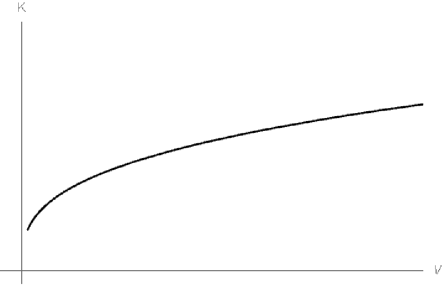
The first derivative of $E(V)$ with respect to the volume defines the pressure of the system, i.e. $P=\frac{dE}{dV}$. In Fig. 7 we see the graphs of the pressure the compression modulus and the energy with respect to the volume for specific regions of the variable $V$. Due to the complicated nature of the relation between $x$ and $V$ it is not easy to put in this parametric plot the behavior of $P$ and $E$ near the region where $V\rightarrow 0$. However, one can calculate through the relations that as one shrinks the volume to zero, the pressure suddenly falls and changes sign becoming negative. The same happens to the compression modulus $\mathcal{K}$ as well, for even smaller values of $V$, while the energy remains positive for all $V$. Unfortunately the expressions are too cumbersome to present them analytically in this work, but the graphs in Fig. 7 demonstrate the general behavior. In the case of a finite cube with $l_{1}=l_{2}=l_{3}$ the situation is a lot simpler as we can see in the following section.

As in [59], we introduce an electromagnetic potential of the form

$$A_{\mu}=(b_{1}(r),0,b_{2}(r),b_{3}(r)),$$

(38)

to be coupled to the multi-Skyrmionic system under consideration. The Maxwell equations (6) reduce to

$$b_{i}^{\prime\prime}=\kappa^{2}M_{ij}b_{j}+\kappa N_{i}$$

(39)

with the nonzero components of $M$ and $N$ being

	$\displaystyle M_{11}$	$\displaystyle=-K\sin^{2}(H)\left[l_{1}^{2}\left(4+\lambda\left(\frac{p^{2}}{l_{2}^{2}}+\frac{q^{2}}{l_{3}^{2}}\right)\cos^{2}(H)\right)+4\lambda H^{\prime 2}\right]$
	$\displaystyle M_{23}$	$\displaystyle=\frac{K\lambda l_{1}^{2}pq}{4l_{3}^{2}}\sin^{2}(2H)$
	$\displaystyle M_{32}$	$\displaystyle=\frac{l_{3}^{2}}{l_{2}^{2}}M_{23}$
	$\displaystyle M_{22}$	$\displaystyle=M_{11}+\frac{p}{q}M_{32}$
	$\displaystyle M_{22}$	$\displaystyle=M_{11}+\frac{q}{p}M_{23}$
	$\displaystyle N_{2}$	$\displaystyle=\frac{p}{4}M_{11}+\frac{1}{4}\left(\frac{l_{3}^{2}p^{2}}{l_{2}^{2}q}-q\right)M_{23}$
	$\displaystyle N_{3}$	$\displaystyle=-\frac{q}{4}M_{11}-\frac{1}{4}\left(\frac{l_{2}^{2}q^{2}}{l_{3}^{2}p}-p\right)M_{32}.$

A direct computation shows that, using the line element in Eq. (16), the three coupled gauged Skyrme equations (namely, $\mathit{E}^{j}=0$, $j=1$, $2$, $3$) in Eq. (5)

$$D^{\mu}\left(R_{\mu}+\frac{\lambda}{4}\left[R^{\nu},G_{\mu\nu}\right]\right)=\mathit{E}^{j}t_{j}=0$$

reduce to only one Skyrme field equation (since the third Skyrme equation is identically satisfied while the first and the second are proportional):

	$\displaystyle\mathit{E}^{3}$	$\displaystyle=$	$\displaystyle 0\ ,$
	$\displaystyle\mathit{E}^{1}$	$\displaystyle=$	$\displaystyle I_{1}P\left[H\right]\ ,\ \mathit{E}^{2}=I_{2}P\left[H\right]\ ,\ \ I_{1}\neq 0\ ,\ I_{2}\neq 0\ ,$

where $I_{j}$ are real and non-vanishing. Thus, the Skyrme field equations reduce to $P\left[H\right]=0$ namely

$$\begin{split}&4\left[X\sin^{2}(H)-\lambda\left(l_{2}^{2}q^{2}+l_{3}^{2}p^{2}\right)-4l_{2}^{2}l_{3}^{2}\right]H^{\prime\prime}+2X\sin(2H)H^{\prime 2}+4\sin^{2}(H)X^{\prime}H^{\prime}\\ &+\Big[\lambda\kappa\left(l_{3}^{2}pb_{2}+l_{2}^{2}qb_{3}\right)\left(-\frac{4l_{1}^{2}p}{l_{2}^{2}}\kappa b_{2}-\frac{4l_{1}^{2}q}{l_{3}^{2}}\kappa b_{3}+2l_{1}^{2}\left(\frac{q^{2}}{l_{3}^{2}}-\frac{p^{2}}{l_{2}^{2}}\right)\right)-\frac{1}{4}l_{1}^{2}X\left(\frac{p^{2}}{l_{2}^{2}}+\frac{q^{2}}{l_{3}^{2}}\right)\\ &+\lambda l_{1}^{2}p^{2}q^{2}\Big]\sin(4H)-\frac{2l_{1}^{2}}{\lambda}X\sin(2H)=P\left[H\right]=0\ ,\end{split}$$

(40)

where

$$X(r)=8\lambda\kappa\left(2l_{2}^{2}l_{3}^{2}\kappa b_{1}^{2}-l_{3}^{2}b_{2}(2\kappa b_{2}+p)+l_{2}^{2}b_{3}(q-2\kappa b_{3})\right).$$

(41)

Quite remarkably, if we demand that

$$X(r)=\lambda\left(l_{2}^{2}q^{2}+l_{3}^{2}p^{2}\right),\quad b_{2}(r)=-\frac{l_{2}^{2}q}{l_{3}^{2}p}b_{3}+\frac{1}{\kappa}\left(\frac{l_{2}^{2}q^{2}}{4l_{3}^{2}p}-\frac{p}{4}\right)\ ,$$

(42)

then the equation for the profile $H(r)$ can be solved explicitly. More importantly, the above algebraic conditions in Eq. (42) are consistent with the Maxwell equations written above. Indeed, if one plugs the two algebraic conditions in Eq. (42) into the three Maxwell equations one obtains a single Maxwell equation for $b_{3}(r)$:

$$b_{3}^{\prime\prime}=\frac{\kappa K}{8l_{2}^{2}l_{3}^{2}}(q-4\kappa b_{3})\left[8\lambda l_{2}^{2}l_{3}^{2}H^{\prime 2}+l_{1}^{2}\left(\lambda\cos(2H)\left(l_{2}^{2}q^{2}+l_{3}^{2}p^{2}\right)+l_{2}^{2}\left(8l_{3}^{2}+\lambda q^{2}\right)+\lambda l_{3}^{2}p^{2}\right)\right]\sin^{2}(H)\ ,$$

(43)

while for the profile $H(r)$ we have a decoupled (from $b_{3}$) equation that reads

$$\left[\lambda\cos(2H)\left(l_{2}^{2}q^{2}+l_{3}^{2}p^{2}\right)+l_{2}^{2}\left(8l_{3}^{2}+\lambda q^{2}\right)+\lambda l_{3}^{2}p^{2}\right]H^{\prime\prime}+\left(l_{2}^{2}q^{2}+l_{3}^{2}p^{2}\right)\left(l_{1}^{2}-\lambda H^{\prime 2}\right)\sin(2H)=0.$$

(44)

Thus, the big technical achievement of the present approach is that the three coupled gauged Skyrme equations in Eq. (5) and the corresponding four Maxwell equations in Eq. (6) with exactly the Skyrme ansatz in Eqs. (12) and (13) and the gauge potential in Eq. (38) reduce to Eqs. (43) and (44) when the two algebraic conditions in Eq. (42) are satisfied. We want to stress that the aforementioned relations provide an exact solution and they are not a product of an approximation. As for the boundary conditions that are needed to be set, we have to keep in mind that the system is confined to a finite box. Thus, the easiest way to realize this is by imposing periodic boundary conditions in $\gamma$ and $\phi$ and Dirichlet in $r$

Interestingly enough, Eq. (44) can be solved explicitly by observing that it has the following first integral

$$Y\left(H\right)\frac{H^{\prime 2}}{2}+V(H)=E_{0}\ ,$$

(45)

with

	$\displaystyle Y\left(H\right)$	$\displaystyle=$	$\displaystyle 2\lambda\left(l_{2}^{2}q^{2}+l_{3}^{2}p^{2}\right)\cos^{2}(H)+8l_{2}^{2}l_{3}^{2},$		(46)
	$\displaystyle V\left(H\right)$	$\displaystyle=$	$\displaystyle-\frac{1}{2}l_{1}^{2}\left(l_{2}^{2}q^{2}+l_{3}^{2}p^{2}\right)\cos(2H)$		(47)

and where $E_{0}$ is an integration constant to be determined by requiring that the boundary conditions to have non-vanishing topological charge are satisfied. Thus, Eq. (44) can be reduced to a quadrature (which defines a generalized elliptic integral). Eq. (43) for $b_{3}$ is linear (since $H(r)$ can be found explicitly), however its integration is not a trivial task. In any case, integration of (43) that results in an expression for $b_{3}$ makes trivial the determination of the other two components of $A_{\mu}$ since both $b_{1}$ and $b_{2}$ are given algebraically in terms of $b_{3}$ through conditions (42). Nevertheless, even without the explicit expressions, it is still possible to analyze the generic features of the transport properties electrons passing through the above gauged Skyrmions.

References

- [1] T. Skyrme, Proc. R. Soc. London A 260, 127 (1961); Proc. R. Soc. London A 262, 237 (1961); Nucl. Phys. 31, 556 (1962).
- [2] T.S. Walhout, Nucl. Phys. A 531, 596 (1991)
- [3] C. Adam, M. Haberichter and A. Wereszczynski, Phys. Rev. C 92, 055807 (2015)
- [4] J.-i Fukuda and S. Žumer, Nature Comm. 2, 246 (2011)
- [5] H. Stefan et al. Nature Physics 7, 713 (2011)
- [6] D. Fostar and S. Krusch, Nuc. Phys. B 897, 697 (2015)
- [7] M. Gillard, Nucl. Phys. B 895, 272 (2015)
- [8] E. Witten, Nucl. Phys. B 223 (1983), 422; Nucl. Phys. B 223, (1983) 433.
- [9] D. Finkelstein, J. Rubinstein, J. Math. Phys.9, 1762–1779 (1968).
- [10] N. Manton and P. Sutcliffe, Topological Solitons, (Cambridge University Press, Cambridge, 2007).
- [11] V. G. Makhanov, Y. P. Rybakov, V. I. Sanyuk, The Skyrme model, Springer-Verlag (1993).
- [12] D. Giulini, Mod. Phys. Lett. A8, 1917–1924 (1993).
- [13] A.P. Balachandran, A. Barducci, F. Lizzi, V.G.J. Rodgers, A. Stern, Phys. Rev. Lett. 52 (1984), 887.
- [14] G. S. Adkins, C. R. Nappi, E. Witten, Nucl. Phys. B 228 (1983), 552-566.
- [15] E. Guadagnini, Nucl. Phys. B 236 (1984), 35-47.
- [16] A. D .Jackson, N. S. Manton and A. Wirzba Nucl. Phys. A 495 (1989) 499.
- [17] C. G. Callan Jr. and E. Witten, Nucl. Phys. B 239 (1984) 161-176.
- [18] J.M. Gipson and H.Ch. Tze, Nucl. Phys. B 183 (1981) 524.
- [19] J. Goldstone and F. Wilczek, Phys. Rev. Lett. 47 (1981) 986.
- [20] E. D’Hoker and E. Farhi, Nucl. Phys. B 241 (1984) 109.
- [21] V.A. Rubakov, Nucl. Phys. B 256 (1985) 509.
- [22] B.M.A.G. Piette, D. H. Tchrakian, Phys.Rev. D 62 (2000) 025020.
- [23] E. Radu, D. H. Tchrakian, Phys. Lett. B 632 (2006) 109-113.
- [24] I. Klebanov, Nucl. Phys. B 262 (1985) 133.
- [25] A. Actor, Phys. Lett. B 157 (1985) 53.
- [26] H. A. Weldon, Phys. Rev. D 26 (1982) 1394.
- [27] M. Loewe, S. Mendizabal, J.C. Rojas, Phys. Lett. B 632 (2006) 512.
- [28] J. A. Ponciano, N. N. Scoccola, Phys. Lett. B 659 (2008) 551.
- [29] M. Kugler and S. Shtrikman, Phys. Rev. D 40 3421 (1989)
- [30] M. Kugler and S. Shtrikman, Phys. Lett. B 208 491 (1988)
- [31] M. Harada, Y.L. Ma, H.K. Lee and M. Rho, Fractionized Skyrmions in Dense Compact-Star Matter, The Multifaceted Skyrmion (second edition), ed. M. Rho and I. Zahed, World Scientific, Singapore (2016)
- [32] Y.-L. Ma and M. Rho, Effective field theories for Nuclei and Compact-Star matter, World Scientific, Singapore (2018)
- [33] L. C. Biedenharn, Y. Dothan, and M. Tarlini, Phys. Rev. D 31, 649 (1985).
- [34] U.-G. Meissner and I. Zahed, Adv. Nucl. Phys. 17, (1986) 143.
- [35] Th. Meissner, F. Grummer, K. Goeke, and M. Harvey, Phys. Rev. D 39, (1989) 1903.
- [36] C. Adam, C. Naya, J. Sanchez-Guillen, J. M. Speight and A. Wereszczynski, Phys. Rev. D 90 (2014) 045003.
- [37] H. Walliser, A. Hayashi and G. Holzwarth, Nucl. Phys. A 456, (1986) 717.
- [38] BES Collaboration, J. Z. Bai et al., Phys. Rev. Lett. 91, 022001 (2003); BES Collaboration, M. Ablikim et al., hep-ex/0503030; BES Collaboration, M. Ablikim et al., Phys. Rev. Lett. 93, 112002 (2004).
- [39] S. Olsen, hep-ex/0305048, invited talk at the International Symposium on Hadron Spectroscopy, Chiral Symmetry and Relativistic Description of Bound States, Tokyo (2003).
- [40] Wang, Z.-G., Eur. Phys. J. A 47, (2011) 71.
- [41] D. G. Ravenhall, C. J. Pethick, J. R. Wilson, Phys. Rev. Lett. 50, 2066 (1983).
- [42] D. Page, S. Reddy, Annu. Rev. Nucl. Part. Sci. (2006) 56: 327–74.
- [43] W. G. Newton, Nature Physics. 9: 396 (2013).
- [44] J. A. Pons, D. Viganò, N. Rea, Nature Physics. 9: 431 (2013).
- [45] D. G. Yakovlev, MNRAS 453, 581 (2015).
- [46] F. Canfora, H. Maeda, Phys. Rev. D 87, 084049 (2013).
- [47] F. Canfora, Phys. Rev. D 88, 065028 (2013).
- [48] F. Canfora, F. Correa, J. Zanelli, Phys. Rev. D 90, 085002 (2014).
- [49] F. Canfora, A. Giacomini and S. Pavluchenko, Phys. Rev. D 90, 043516 (2014).
- [50] S. Chen, Y. Li, Y. Yang, Phys. Rev. D 89 (2014), 025007.
- [51] E. Ayon-Beato, F. Canfora, J. Zanelli, Phys. Lett. B 752, (2016) 201-205.
- [52] F. Canfora, M. Di Mauro, M. A. Kurkov, A. Naddeo, Eur. Phys. J. C (2015) 75: 443.
- [53] F. Canfora, G. Tallarita, Nucl. Phys. B 921 (2017) 394.
- [54] F. Canfora, G. Tallarita, Phys. Rev. D 94, 025037 (2016).
- [55] F. Canfora, G. Tallarita, Phys. Rev. D 91, 085033 (2015).
- [56] F. Canfora, G. Tallarita, JHEP 1409, 136 (2014).
- [57] F. Canfora, Seung Hun Oh, P. Salgado-Rebolledo, Phys. Rev. D 96 (2017), 084038.
- [58] P. D. Alvarez, F. Canfora, N. Dimakis and A. Paliathanasis, Phys. Lett B. 773, (2017) 401-407.
- [59] L. Aviles, F. Canfora, N. Dimakis, D. Hidalgo, Phys. Rev. D 96, (2017) 125005.
- [60] H. Weigel, Chiral Soliton Models for Baryons, Lecture Notes in Physics (Springer, 2008).
- [61] F. Wilczek, Phys. Rev. Lett. 109, 160401 (2012).
- [62] A. Shapere, F. Wilczek, Phys. Rev. Lett. 109, 160402 (2012).
- [63] F. Wilczek, Phys. Rev. Lett. 111, 250402 (2013).
- [64] K. Sacha, J. Zakrzewski, ”Time crystals: a review” arXiv: 1704.03735.
- [65] Y. M. Shnir, Magnetic Monopoles (Springer-Verlag, Berlin, Heidelberg, 2005) pp.500
- [66] G. E. Brown and E. Osnes Phys. Lett. B 159 (1985) 223-227
- [67] G. Co’ and J. Speth Phys. Rev. Lett. 57 (1986) 547-550
- [68] J. P. Blaizot, Phys. Rep. 64 (1980) 171-248
- [69] M. E. Caplan and C. J. Horowitz, Rev. Mod. Phys. 89 (2017) 041002.
- [70] M. Dutra, O. Lourenço, J. S. Sà Martins, A. Delfino, J. R. Stone and P. D. Stevenson, Phys. Rev. C 85 (2012) 035201
- [71] M. Dressel and G. Grüner, Electrodynamics of Solids (Cambridge University Press, Cambridge, 2002).