Local Stability of Galactic Discs in Modified Dynamics2018Local Stability of Galactic Discs in Modified Dynamics–12
Abstract
The local stability of stellar and fluid discs, under a new modified dynamical model, is surveyed by using WKB approximation. The exact form of the modified Toomre criterion is derived for both types of systems and it is shown that the new model is, in all situations, more locally stable than Newtonian model. In addition, it has been proved that the central surface density of the galaxies plays an important role in the local stability in the sense that LSB galaxies are more stable than HSBs. Furthermore, the growth rate in the new model is found to be lower than the Newtonian one. We found that, according to this model, the local instability is related to the ratio of surface density of the disc to a critical surface density . We provide observational evidence to support this result based on star formation rate in HSBs and LSBs.
Keywords:
instabilities – galaxies: kinematics and dynamics – galaxies: spiral , galaxies: star formation – methods: analytical – methods: data analysis.1 Introduction
The star formation rate (SFR), which is a key factor in understanding galactic evolution, is usually approximated by empirical power law of 1959, which states that . Here, is the SFR per surface density, is the gas surface density and . 1989; 1998 shows that this law breaks down at densities below a critical threshold value. He also fits the law to a sample of star-forming discs of spiral and starburst galaxies and concludes that for his sample. See also 2011 for a review on empirical laws of SFR on galactic scales. On the other hand, gravitational instabilities are usually considered as the source of star formation and there have been many attempts to relate the instabilities to SFR (1994; 1996). Unfortunately though, such attempts are usually faced with difficulties due to little understanding of the star formation at small scales, i.e. the physics of the clouds (2007; 1994). However, one could always hope for an overall correct behaviour derived from gravitational instabilities at larger scales, assuming that the effects of small scale physics could be averaged.
Gravitational instabilities was first studied in detail by 1960 who showed that instabilities can occur in a rotating disc of fluid. For the case of stellar discs too, 1964 derives a stability criterion for a razor-thin disc. One key feature in studying gravitational instabilities is the assumption that wavelength of the perturbation is much smaller than the size of the system, an approximation which is known as WKB or tight-winding approximation (1964).
There have been many attempts to make the single fluid or stellar models more realistic. For example, the effect of the thickness of discs is derived by 1970 while stellar plus gas systems have been considered by 1972; 1984. Also, a simple stability criterion for stellar plus gas systems has been proposed by 1994 and generalized by 2011. See also 1995 and 1996. Moreover, 2001 has studied the gravitational stability of systems with several stellar components plus a gas component. All the above mentioned studies have assumed Newtonian force as the governing law of gravitation. Therefore, even with the introduction of a massive halo surrounding a galaxy ( the CDM picture of galactic dynamics), the main features and conclusions of gravitational instabilities will remain intact 2014.
The standard model of cosmology, i.e. the model, has been very successful in explaining key properties of galactic and extra galactic scales, though, the most prominent problem of this model is still the detection of the dark matter particle. On the other hand, there have been some attempts to justify galactic dynamics, not by putting more mass to the systems, but by modifying the law of gravity. In this method, the modifications that one introduces to the theory of gravity results in conversion of the force law or the inertia term. For the latter, the most famous model is MOND by 1983a; 1983b; 1983c while for the former, among many other theories, one could mention Scalar-Tensor-Vector theory of 2006 (known also as MOG) and the well-known theories (2010). Among all different proposals to modify gravity, MOND is especially interesting because this model unifies different aspects of galactic dynamics by introducing a single parameter which has the dimension of acceleration. See 2012 for a thorough review on MOND implications, applications and difficulties.
Theories of modified gravity have to be consistent with the data at different scales. In the case of theories, in which is the Ricci scalar, 2010 have explained that to fit the rotation curve data, the parameter should depend on the mass of individual galaxies. Thus, one concludes that it is not possible to fit the data for all galaxies with the same choice of . On the other hand, as 2012 have discussed extensively, although MOND provides a powerful alternative in studying rotationally supported systems, its success in pressure-supported systems is concluded as "less impressive" or even "really problematic" in some cases (e.g. galaxy clusters). Moreover, MOG explains the rotation curve of spirals (2013) while displays large mass-to-light ratios for dwarf spheroidal (dSph) galaxies (2016). In addition, concerning the physics of the solar system, some theories violate the current bounds on the perihelion precession of several planets (2007; 2008) while MOND (2009) and MOG (2008) pass this test.
Except for consistency with observational data, modified gravities/dynamics with less free parameters are generally more favoured within the community. In fact, 2010 report that the success of model is based on the fact that only a handful of parameters are required to fit observations. Also, some modified theories show difficulties in dealing with their mathematical structures. For instance, the non-linearity of MOND makes it difficult to derive analytical solutions for the model; though, one could solve the equations numerically (2012). The mathematical simplicity of models usually leads to easier interpretations of physical consequences; though, there is no guarantee that the final model must be necessarily simple.
The problem of local stability of galactic discs in modified theories provides a powerful tool in studying the behaviour of these theories. For example, 1989 investigates local stabilities of discs governed by MOND dynamics, 2014; 2015a study the effects of MOG while the implications of have been surveyed by 2015b. Also 2016 and Ghafourian & Roshan 2017 study the global stability of galactic discs under MOG from theoretical and numerical point of view respectively.
The aim of this work is to study the theory of local stability, and its observable implications, in a modified dynamical model. In the next section we will review this modified model which is based on changing boundary condition of general relativity (GR) from Dirichlet to Neumann (2016a; 2016b). In sections three and four the local stability criterion, growth rate and neutral stability curves are derived for fluid and stellar discs respectively. Most of the physical discussions and observable implications are postponed to Sec. 5 in which we use 2008 data to test the reliability of the model.
2 Modified Dynamics, A Review
The model which we discuss here, has been derived by assuming a Neumann boundary condition on GR perturbation equations in an expanding universe. See 2016a for the details. Recently, it has been shown that the surface term of GR action identically vanishes if we assume Neumann boundary condition (2016; 2016). 2016a have also reported an alternative path integral for quantum gravity using Neumann BC. Furthermore, it could be shown that a natural BC for gravity in asymptotically AdS spaces is to hold the renormalized boundary stress tensor density fixed instead of fixing the boundary metric (2016b).
2016a imposes Neumann boundary condition on cosmic perturbation equations, i.e. essentially Taylor expansion of Einstein field, and derives a modified Friedmann and lensing equations. The reliability of the new lensing equation has been checked by a sample of ten strong lensing systems (2016a). This new model predicts a constant acceleration in the equation of motion as in which is the Neumann constant and . Here is the speed of light and is the Hubble constant. Using this new model one could show that the growth of structures in matter dominated era is more rapid than the standard model (2016a).
In addition, 2016b shows that the new term in the equation of motion suggests a small, though detectable, correction in perihelion precession of planets. Furthermore, for a system of particles with mass distribution and total mass of M it was shown that the total modified potential is as follows
| (1) |
in which the first term on the rhs is the gravitational potential of Newtonian theory while the second one is due to imposing Neumann BC to GR perturbation equations. A potential similar to the second term has been previously named "superpotential" by 1962a; 1962b; 1962c. In fact, these authors have surveyed many properties of this superpotential in the aforementioned papers.
The Poisson equation, with which one could start solving many problems in classical mechanics, is modified in this model. In fact, it is easy to derive the next second order Integro-differential equation
| (2) |
as the modified Poisson equation. However, as it is discussed in 2018, one could see that the next fourth-order Poisson equation
| (3) |
is usually more suitable to use in analysis for the simple fact that it is only differential. In this work too, we will use the fourth-order Poisson equation more often than the second order one. The homogeneous form of Eq. (3) is known as biharmonic equation which rises mostly in the theory of linear elasticity. To solve this equation, one needs four boundary conditions. See 2000, chapter 8, for a thorough review on different solutions of the biharmonic equation. In addition, 1988 present a survey on the existence and uniqueness of solutions of the biharmonic equation.
For a razor-thin disc galaxy with cylindrical symmetry and radius , if one assumes an exponential profile for the mass distribution
| (4) |
then it is possible to derive the rotation curve formula by applying 1983 and 2006 method which is based on direct integration of the potential and using Bessel function expansion of Green function in cylindrical coordinates. By doing so, one could find (2016b)
| (5) |
in which is the scaled radius and is a fundamental surface density in this model which has been previously argued to be an upper limit for the surface density of spirals (1989). See 2012 for more discussions on this limit. The value of is about which is very close to the observational value for central surface brightness of spiral galaxies reported by 1970. Now, however, this is known as a maximum surface density limit above of which the disc galaxies are very rare. See, for instance, 1989; 1996; 2012 and Sec. 5 below for more details. Almost all of our following results show a dependency to this ratio which we call Freeman ratio .
Neglecting vertical thickness of the objects, from Eq. (5) one could see that galaxies with high values of should show rising rotation curves, those with intermediate values of should show a constant circular velocity while objects with the smallest values of possess declining rotation velocities. Including the thickness of the objects typically decreases the circular velocity. See 2018 for the proof of this statement. A similar result is reported by 1991 who show that the rotation curve of low luminosity dwarf galaxies, with maximum velocity lower than about 100 km/s, are generally rising. Also, the velocities of intermediate to high luminosity galaxies, with velocities respectively in the range of and , are typically flat. But, the rotation velocities of the very highest luminosity galaxies are found generally to be declining from 15 for NGC2903 to 30 for NGC2683. See 2016b for the data fitting of 39 LSB galaxies for which it is shown that the rotation curve fittings are generally acceptable.
As we know, the solution to any differential equation, including Einstein field equations, depends on both the functional form of the equation and its boundary condition. The core idea of the present model is to impose Neumann BC, i.e. , on Einstein field equations (2016a) instead of changing the basic action of GR as it is common in theories of modified gravity. There are some advantages in this approach, the first of which is that, by doing so the unique Einstein-Hilbert action remains intact. Second, by assuming Neumann boundary condition the surface term of GR action identically vanishes. This could somehow settle the long-time debate on the surface term of GR if this assumption leads to a successful cosmological model. Third, because the new term in the equation of motion is of the order of the fundamental parameter of MOND, i.e. , the dynamical predictions of the present model too would scale ( in data analysis ) by a similar constant acceleration . Therefore, the success of the present model in matching observational data could provide a physical interpretation for the clear success of the MOND phenomenology. Fourth, a possible link between local and global physics has been debated for a long time but never been answered thoroughly. See 2016a for a review on this matter from 1945 model to contemporary era. The present model provides another method to build such connection with the possibility to test it with a large amount of observational data at galactic and extragalactic scales. In the following, for instance, we consider the local stability of disc galaxies and we will see that in this model the local stability is correlated with global expansion of the universe through the parameter .
The present model is clearly linear which is a great advantage in analyzing its results. In fact, this property helps to perform the analytical calculations through extending the results of the Newtonian theory in a straightforward manner. For example, we will see in the following that the local stability criterion of stellar and fluid systems could be derived. In addition, the present model is built based on only one free dimensionless parameter, i.e. , which could be determined by observations. Thus, this model is quite economical in introducing new parameters.
We will see below that in the present model, the local stability is crucially dependent to . Also, it is found that galaxies with low are more unstable than galaxies with high . Thus, one should observe that HSB galaxies are more unstable than LSBs. The observational evidence to support this prediction will be presented in Sec. 5 which is dedicated to data analysis.
3 Modified Dispersion Relation for a Fluid Disc
In a fluid disc, the combined stabilizing effects of pressure and angular momentum are in competition with the force of gravity which always wants the system to collapse. In a Newtonian model, if the stabilizing effects are dominant, i.e.
| (6) |
then the system would be stable against local collapse (1960). In the last equation, is the epicyclic frequency which, by using angular velocity , is defined as follows
| (7) |
while is the sound speed in the fluid and is the disc surface density. One may see 1964 or 2008 page 443 for a physical interpretation of this stability criterion in the context of Newtonian dynamics.
In the context of dark matter model, 2014 have noticed that the square of the total epicyclic frequency of a disc surrounded by a halo could be written as . See Eqs. (17) and (21) of 2014 for the exact form of ( for pseudo-isothermal halo ) and . The presence of the halo would lead to a higher net and hence a higher which results in a more stable system. In accordance with 2014, we will rewrite the net epicyclic frequency square as where represents the epicyclic frequency due to Newtonian force which is the same as from 2014 while is resulted from the new term in our modified equation of motion. Due to the existence of the latter term in the present model, the stabilizing effect of angular momentum is strengthened; thus, one expects a more stable model compared to pure Newtonian one.
To derive the exact stability criterion in any modified dynamics, one needs the continuity equation , the Euler equation and also the modified Poisson’s equation which was introduced in the previous section. We will follow the method by 2008 which is effectively summarized and simplified by 2015a. The general idea is that one first finds the solution to the Poisson equation for a disc and then puts these solutions into the first order approximation of continuity and Euler equations. A barotropic equation of state, i.e. in which and are real constants, is also assumed here. The system is considered to be an axisymmetric and razor-thin disc. We will use non-rotating cylindrical coordinates with as the rotation axis, while and show radial and azimuthal coordinates respectively. Our notation mostly follows 2008.
To linearise the governing equations, we assume that , , , and the specific enthalpy in which 0 and 1 indices represent zeroth-order and first order perturbations respectively. By putting these parameters into the continuity equation and Euler equations, one can rewrite the governing equations as (2008; 2015a):
| (8) |
In addition, by assuming that all perturbations could be approximated locally by a plane wave, i.e. in which could be any of the perturbations while is the radial wavenumber, and also by presuming WKB approximation , it is possible to significantly simplify Eqs. (8).
The WKB approximation, also known as tight winding approximation, is assumed to remove the long-range feature of the gravitational force and so it makes the equations local. In this approximation, the radius of the system is much larger than the radial wavelength; thus, it is possible to omit terms proportional to comparing to the terms proportional to the wavenumber . Applying this approximation, one can simplify Eqs. (8) as
| (9) |
in which and are both functions of radius, known as Oort’s parameters, while is the amplitude of the specific enthalpy.
The next step is to find the solution to the first order modified Poisson equation. We use fourth order Poisson equation (3) instead of the second order Eq. (2) essentially because dealing with a pure differential equation is much easier than dealing with an integro-differential equation; though, in Eq. (3) one deals with four boundary conditions instead of two. Here we are seeking the solutions to Eq. (3) when in which . Assuming without loosing generality that the initial perturbation is in the direction, one can propose , in which is a constant, to solve the modified Poisson equation. Because there is no mass outside of the plane of the disc, i.e. when , one can readily show that for these points . However, in such system the vertical component of the force is discontinuous in the plane of the disc. Therefore, to find the solution we integrate Eq. (3) with respect to parameter . The interval of the integration is . See 2008, chapter two, for a similar treatment of the Newtonian case. The disc is supposed to be razor-thin; therefore one could find the lhs of Eq. (3) by taking the limit when as
In the second row of the above equation we have used the fact that the proposed potential is independent of and continuous with respect to while in the third row we have differentiated with respect to and and also have done the integration. To obtain the solution to the biharmonic equation, i.e. Eq. (3), we have used the boundary values of and at while, because of the symmetry, the second order derivative is absent from the evaluation on the third row. In addition, the boundary condition on the value of the potential is as which has been implicitly applied before, when we assumed the same amplitude for both sides of the sheet.
The rhs of Eq. (3) is more straightforward, though one should note that the terms proportional to derivatives of the Dirac delta function converge to zero because . The final answer is as follows
| (10) |
from which the potential amplitude is read as
.
Now, if we substitute into the second equation of (9), we would be able to derive the radial velocity as
| (11) |
By replacing from the last equation into the first equation of (9) one could find the dispersion relation as
| (12) |
where in the case of axisymmetric disturbances , which is the main focus of the present work, becomes
| (13) |
We should point out that considering the above relation reduces to the Newtonian counterpart as we expected. Regarding Eq. (13), a perturbation with the time dependency proportional to would oscillate forever if is real, or equivalently , and such system would be stable. However, if then would be a complex number; consequently the perturbation would grow exponentially and thus the system would be unstable.
The modifications that the present model introduces to the problem of local stability could be well understood by considering the last factor in Eq. (13), i.e. . This factor introduces a boundary wavenumber as below of which is negative and above of that is positive. Now, because the first two terms on the rhs of Eq. (13) are positive, if then and the system is stable against the perturbation with wavenumber . On the other hand, if then the last term on the rhs of Eq. (13) would be negative and there would be a competition between stabilizing effects of angular momentum and pressure, i.e. , and destabilizing effect of gravity. Anyway, in the latter case if gravity won and the system became locally unstable, the unstable modes would grow with a lower rate compared to the pure Newtonian model because the factor reduces the destabilizing effect of gravity as it is clear from Eq. (13).
In what follows in this section, we will try to demonstrate the different aspects of Eq. (13) in more precise details. The modified Toomre’s criterion, i.e. the local stability criterion, could simply be derived and analysed if we define the dimensionless wavenumber and the parameter as
| (14) |
Using these parameters, we rewrite the dispersion relation (13) as the following equation
| (15) |
in which is the Newtonian Toomre parameter for a fluid disc which is defined by Eq. (6). It is now easy to see that one could use the dispersion relation (15) to rewrite the stability criterion, i.e. , as the following equation
The rhs of the last inequality is dependent to the dimensionless wavenumber . To find a stability criterion independent of we argue that if is larger than the maximum value of the rhs of the last equation, then the system is stable for any value of . Thus we rewrite the last equation as
| (16) |
in which represents maximization with respect to .
In the case of fluid disc it is possible to find the result of this maximization process analytically. To find the maximum of the rhs of Eq. (16), we will differentiate the rhs with respect to . By finding the roots of the result of this differentiation one finds where has been introduced for the sake of brevity. Two of the roots are complex numbers for any ; thus they are dismissed. The other two roots are the same within a minus sign . This is in fact the value of the wavenumber at which the system is closest to being unstable. For this root, the maximum value of the rhs of Eq. (16) could be found and thus the stability criterion for fluid disc be rewritten as:
| (17) |
In this way, the stability criterion is written in a way which is manifestly independent of . One could easily check that the rhs of Eq. (17) is a decreasing function of . Also, we notice that for , i.e. the Newtonian theory, one finds and as it is expected. In addition,
through dependency of the parameter to and Freeman ratio , we could see that the stability criterion (17) is solely dependent to the location of the point under consideration and the relative surface density of the galaxy.
The above results could be obtained from another perspective too. As 1984; 1996 have argued, for a system to be in neutral equilibrium, the equations and must have a simultaneous real solution for the wave number . By doing so, one could derive the same as above and from that the stability criterion Eq. (17) would emerge. We do not perform this calculation here for the sake of brevity.
Now we give an estimation of the magnitude of . In the solar neighbourhood, for instance, we have and while the radius of the Milky Way is estimated to be about . Thus, in our neighbourhood we could safely assume that . For more interior positions, might rise significantly while the velocity dispersion in the gas is still of the same magnitude as before. Thus might be much less than 0.1. On the other hand, in the case of smaller galaxies we have , but then the ratio of decreases too as we will see in the section for data analysis below. Therefore, we consider this parameter to be in the range of and we find the maximum value of the rhs of Eq. (16).
The results of this maximization procedure are reported in Tab. 1 for different values of and . For the Newtonian case, i.e. , it is natural to find the maximum value of the rhs of (16) equal to 1. This is evident from Eq. (16) even without any numerical maximization. Also we see that when is relatively small, for example , the maximum value is always the same as the Newtonian case. On the other hand, when increases the maximum value decreases. Thus, regions with larger are more stable than others. In addition, low surface brightness galaxies (LSB), i.e. those galaxies with higher ratio of , ought to be more stable than HSBs because the maximum value of (16) is smaller when is large. Although to see this vividly, one needs to find places with a higher value of .
| Fluid Systems | Stellar Systems | |||||
|---|---|---|---|---|---|---|
| 1.00 | 1.00 | 1.00 | 1.00 | 1.00 | 1.00 | |
| 1.00 | 1.00 | 0.99 | 1.00 | 1.00 | 0.98 | |
| 1.00 | 1.00 | 0.88 | 1.00 | 1.00 | 0.87 | |
| 1.00 | 0.96 | 0.53 | 1.00 | 0.96 | 0.48 | |
| 1.00 | 0.93 | 0.40 | 1.00 | 0.92 | 0.36 | |
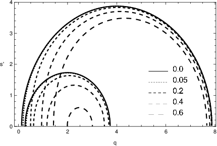
The neutral stability curves, i.e. the curves corresponding to , are interesting too. From Eq. (15) one could see that defining the dimensionless wavelength , in which , these curves could be found as
| (18) |
In this equation is in fact resembling Tully-Fisher relation because it includes on one hand the velocity to the power of four, i.e. , and on the other hand the total mass of the system . However, we do not expect that be very close to 1 since for the most parts of the galaxies would not be the same as flat velocity of the system, for which the Tully-Fisher relation is defined. Fig. 1 shows the neutral stability curves versus for different values of . The Newtonian case, which corresponds to , is the most unstable case while by increasing the magnitude of more and more regions become completely stable.
2018 derives the Tully-Fisher relation for the present model as alongside with three other major scaling relations. Here and are some dimensionless Virial coefficients while represents the flat velocity. See 2018 for more details about the general form of the scaling rules in this model and their test based on data analysis.

Unstable modes, i.e. modes with , show interesting features too. Defining the dimensionless growth rate parameter as , one could see that Eq. (15) can be rewritten as
| (19) |
This quantity has been plotted in Fig. 2 as a function of dimensionless wavenumber for a fixed Freeman ratio and different values of and . The growth rate decreases by increasing both and . The growth rate in the present model is vividly lower than the Newtonian case.
The effect of the parameter on the disc’s stability is also evident from Fig. 2. It is seen that higher values of , which happens where the dynamical velocity is comparable to the sound velocity, results in a more stable condition. This is compatible with the observations since, as we will see later, is lower in the outer parts of the galaxy while is considered to be almost constant throughout the galaxy; thus, the parameter would have a higher value in such regions. Therefore, in the outer parts of the galaxy the stability against local perturbations is stronger, which results in a lower star formation.
4 Modified Dispersion Relation for a Stellar Disc
According to 1964, a stellar disc in Newtonian gravity would be stable if
| (20) |
in which, again, the stabilizing effects of angular momentum and velocity dispersion in the radial direction are competing with destabilizing force of gravity. To find the local stability criterion of stellar discs in a modified gravity/dynamics, one needs the collisionless Boltzmann equation
| (21) |
and also the modified Poisson equation (2). The derivation here is similar to the previous section, though, for the reason that the disc is not completely cold, one could not derive by simply putting in the second equation of (9). See 2008 pages 492-495. However, 1964 has shown the existence of a partial cancellation due to the effects of the spiral potential on , i.e. the mean velocity perturbation. This cancellation reduces the value of by a factor of , known as the reduction factor, as
| (22) |
For a thorough review on reduction factor and its formal derivation for a razor-thin disc see 2008 appendix K. The general form of the factor is independent of the form of Poisson equation (2014). Therefore, it shows the same dependencies on dimensionless frequency and wavenumber and could be written as
| (23) |
in which and .
If we replace from Eq. (22) into the first equation of (9), which by the way remains unchanged, one could derive the following dispersion relation
| (24) |
for the stellar disc. Here, we also assume axisymmetric perturbations, for which , and so
| (25) |
Recalling the boundary wavenumber , the rhs of Eq. (25) is positive, if . Thus, in this case and the system is stable against local perturbations. On the other hand, if then the second term on the rhs of Eq. (13) would be negative and there is a competition between stabilizing effect of angular momentum and velocity dispersion on one hand, and destabilizing effect of gravity on the other hand. The stabilizing effect of velocity dispersion is included in . Anyway, if gravity wins and the system became locally unstable, the unstable modes grow with a lower rate, compared to the pure Newtonian model, because the factor decrease the effect of gravity as we see from Eq. (25).
Now we derive the modified Toomre’s criterion, neutral stability curve and growth rate for the stellar model. Defining dimensionless parameter as
| (26) |
one can rewrite the above dispersion relation as follows
| (27) |
The maximum value of the rhs of the above equation occurs at . Now, if the rhs is smaller than 1 when , then there would be no imaginary solution for . In this case, the local perturbation could not destabilize the disc and the disc would be stable. Thus, for a typical wavenumber the above equation could be rewritten as
To eliminate the dependency on , we notice again that if in the above inequality was larger than the maximum value of the rhs, then the system would be stable for any value of . Therefore, we rewrite the modified Toomre’s criterion for the stellar system as
| (28) |
or equivalently, by using modified Bessel function expression of the reduction factor, i.e. , see 2008 page 833, one could derive a more practical form as
| (29) |
One could easily check that, unlike the fluid disc, the maximization process could not be performed analytically due to complicated dependency of Bessel function to the wavenumber through the term . However, the numerical maximization is always possible as we will see in the next section.

The growth rate of the unstable modes of stellar discs, i.e. , is studied by using Eq. (25). The result is plotted for different values of as a function of dimensionless wavenumber in Fig. 3. It should be mentioned that in this figure, two different values for is considered and it is obvious that similar to the fluid case, the growth rate of the instability is higher for lower values of Toomre parameter. Comparing this plot with Fig. 2 also shows that stellar systems, if unstable, generally collapse with a lower rate than gaseous systems.
As described before, one could also derive the neutral curves, which are the boundary of stable and unstable modes, from the condition . Defining for the sake of simplicity a new parameter , it is possible to rewrite the dispersion relation (25) as
| (30) |
and then plot as a function of . The result is plotted for different values of by solid lines in Fig.1. The most unstable case is the Newtonian model with . In addition, with increasing the disc becomes more stable against perturbations with large wavelength . In other words, for higher values of the total area of instability in plane decreases. Also, the neutral curves of stellar and fluid discs are very similar, though, the peak of the fluid model occurs at a smaller with a slightly larger value.
The maximum values of Eq. (28), for different Freeman ratios and , are reported in Tab. 1. In this table we see that when , and for the same Freeman ratio , the maximum values of the stellar systems are slightly lower than fluid ones. From Fig. 1 too, one could see that the area of instability region of the fluid system is slightly larger than the stellar one with the same parameter . On the other hand, the Newtonian model shows a symmetrical behaviour around for stellar and fluid discs. Thus, one could conclude that in the present model, assuming WKB approximation, the stellar systems are more stable against local axisymmetric perturbations than fluids with same interim parameters. However, as we will show in the next section, for most galaxies is an order of magnitude smaller than ; thus, the condition does not hold in most points of the discs. In addition, to draw a more accurate conclusion about the stability of galactic discs, one needs to treat the galactic discs as a combination of stellar plus fluid systems. We will discuss about this last point in the next section. Moreover, below we will briefly consider the stability of stellar and gaseous discs against non-axisymmetric disturbances independent of parameters.
It is also possible to use the dispersion relations of fluids and stellar discs to study the behaviour of the dimensionless frequency, i.e. in which is the pattern speed of an m-armed spiral, for non-axisymmetric disturbances . See 2008, page 497, or 2015. One expects the present model to show a different behaviour at very long ranges, i.e. when approaches to zero, compared to the Newtonian model because the gravitating force of the present model is stronger than the Newtonian one. In addition, stellar and fluid systems should have similar trends, because in this regime, the dominant force is gravity while the pressure or velocity dispersion are negligible. From mathematical point of view one could see that for small we have in which is the dimensionless wavenumber ( ). Thus, we conclude that in the present model the dimensionless frequency diverges when tends to zero. Accidentally, this is the region that the WKB approximation fails; thus, a definitive conclusion needs to go beyond this approximation.
Moreover, it could be shown that for large wavenumber , the dimensionless frequency of the stellar systems approaches to (the Lindblad resonances) while it grows indefinitely for the fluid systems. In this sense, the present model resembles the Newtonian one which is a predictable behaviour because at large the dominant factor is no longer self-gravity but pressure - for fluids - or velocity dispersion - for stellar systems - which both remain unchanged in our model. This behaviour shows that at high fluid systems are more bouncy compared to stellar systems; thus, former discs are more stable against non-axisymmetric perturbations . The stability of galactic systems against non-axisymmetric disturbances needs more careful treatments, though one could see 2001; 2015 for thorough investigations on physical implications of this matter in Newtonian gravity.
In the context of dark matter paradigm too, 2014 have shown that gravitational instabilities are suppressed in the case of LSBs dominated by their haloes. They have tested their results for the LSB galaxy UGC 7321, a superthin disc with well-documented observational parameters. The stability of this galaxy against local, linear axisymmetric and non-axisymmetric perturbations has been studied (2014). In conclusion, it is proved that in LSBs the star formation and spiral features are mainly suppressed due to the dynamical effect of the halo dominating from inner regions. The local stability of a two-component disc has been shown by 2014 too.

5 Data Analysis and Discussion
In this section, we will use data from 2008 to compare the local stability of the present model with a second one. Our second model, hereafter named model II, assumes Toomre criterion for which the net epicyclic frequency is derived based on 2003 rotation curve formula. 2008 use 2003 proposal which describe rotation velocity as a function of radius as
| (31) |
In this formula is the velocity at which the rotation curve is flat while is the length scale for which rotation curve begins to be flat. These parameters, for every galaxy in our sample, are reported in Table. 2 as derived by 2008. Of course, from the context of the dark matter hypothesis, the flatness of at large radii is due to the existence of a dark halo. In the presence of a halo, the general form of the Toomre criterion, i.e. , remains unchanged; though, the is derived by combining the contributions from the disc and the halo as explained in Sec. 3 above. See Eq. (17) of 2014, for example. However, 2014 derives the contribution of a pseudo-isothermal halo from first principles.
2008 use HI maps from THINGS ( The HI Nearby Galaxy Survey) and also derive maps. The global properties of this sample which includes 23 galaxies are introduced in Tab. 2. We particularly try to find a correlation between the gravitationally unstable positions of the galaxies and their star formation rate surface density . 2008 use maps of far-ultraviolet (FUV) combined with 24 maps to find a tracer sensitive enough to both exposed and dust-embedded star formation. This results in a good measure for in units of . They derive the data related to FUV from 2007. Since very massive young stars are emitting their energy mainly through ultraviolet emission, FUV provides a prominent measure for the rate of star formation.
| Name | Type | SFR | ||||||||||||
| (kpc) | (kpc) | (kpc/s) | (kpc) | (kpc) | ||||||||||
| NGC7331 | SAb | 19.6 | 10.9 | 10.1 | 9.7 | 1.3 | 244 | 3.3 | 2.987 | 4.5 | 117. | 0.18 | 0.26 | 0.86 |
| NGC6946 | SBc | 9.8 | 10.5 | 9.8 | 9.6 | 1.4 | 186 | 2.5 | 3.239 | 2.7 | 67.7 | 0.25 | 0.20 | 0.98 |
| NGC5194 | SBc | 9. | 10.6 | 9.5 | 9.4 | 0.8 | 219 | 2.8 | 3.125 | 2.4 | 52.6 | 0.12 | 0.17 | 0.90 |
| NGC5055 | Sbc | 17.4 | 10.8 | 10.1 | 9.7 | 0.7 | 192 | 3.2 | 2.123 | 3.1 | 110.9 | 0.22 | 0.15 | 0.93 |
| NGC4736 | Sab | 5.3 | 10.3 | 8.7 | 8.6 | 0.2 | 156 | 1.1 | 0.481 | 0.9 | 39.8 | 0.04 | 0.51 | 0.99 |
| NGC3627 | SBb | 13.9 | 10.6 | 9. | 9.1 | 1.2 | 192 | 2.8 | 2.217 | 1.9 | 135.8 | 0.05 | 0.07 | 0.69 |
| NGC3521 | SBbc | 12.9 | 10.7 | 10. | 9.6 | 1.4 | 227 | 2.9 | 2.104 | 3.1 | 76.7 | 0.22 | 0.21 | 0.88 |
| NGC3351 | SBb | 10.6 | 10.4 | 9.2 | 9. | 0.7 | 196 | 2.2 | 0.94 | 1.8 | 119.9 | 0.09 | 0.95 | 0.98 |
| NGC3198 | SBc | 13. | 10.1 | 10.1 | 8.8 | 2.8 | 150 | 3.2 | 0.931 | 3.4 | 193.6 | 0.51 | 0.93 | 0.43 |
| NGC3184 | SBc | 11.9 | 10.3 | 9.6 | 9.2 | 2.8 | 210 | 2.4 | 0.901 | 2.8 | 164.1 | 0.22 | 0.46 | 0.77 |
| IC2574 | Irr | 7.5 | 8.7 | 9.3 | 7.9 | 12.9 | 134 | 2.1 | 0.07 | 4.8 | 645.6 | 0.81 | 3.07 | 0.81 |
| NGC628 | Sc | 10.4 | 10.1 | 9.7 | 9. | 0.8 | 217 | 2.3 | 0.807 | 2.4 | 171.9 | 0.32 | 0.38 | 0.84 |
| NGC925 | SBcd | 14.2 | 9.9 | 9.8 | 8.4 | 6.5 | 136 | 4.1 | 0.561 | 4.1 | 411. | 0.45 | 1.18 | 0.53 |
| NGC2403 | SBc | 7.3 | 9.7 | 9.5 | 7.3 | 1.7 | 134 | 1.6 | 0.382 | 2. | 192.3 | 0.39 | 0.36 | 0.84 |
| NGC2841 | Sb | 14.2 | 10.8 | 10.1 | 8.5 | 0.6 | 302 | 4. | 0.741 | 5.3 | 78.4 | 0.17 | 0.37 | 0.78 |
| NGC2976 | Sc | 3.8 | 9.1 | 8.3 | 7.8 | 1.2 | 92 | 0.9 | 0.087 | 0.8 | 280.6 | 0.17 | 0.36 | 0.79 |
| NGC3077 | Sd | 3. | 9.3 | 9.1 | 6.5 | - | - | 0.7 | 0.086 | 0.3 | 81.7 | 0.39 | 0.21 | 0.4 |
| NGC4214 | Irr | 2.9 | 8.8 | 8.7 | 7. | 0.9 | 57 | 0.7 | 0.107 | 0.5 | 217.7 | 0.45 | 0.37 | 0.4 |
| NGC4449 | Irr | 2.8 | 9.3 | 9.2 | 6.9 | - | - | 0.9 | 0.371 | 0.8 | 64.6 | 0.44 | 0.43 | 0.73 |
| NGC7793 | Scd | 6. | 9.5 | 9.1 | 0 | 1.5 | 115 | 1.3 | 0.235 | 1.3 | 240.7 | 0.28 | 0.29 | 0.80 |
| DDO154 | Irr | 1.2 | 7.1 | 8.7 | 6.8 | 2. | 50 | 0.8 | 0.005 | 1. | 81.9 | 0.98 | - | - |
| HoI | Irr | 1.8 | 7.4 | 8.3 | 7.2 | 0.4 | 53 | 0.8 | 0.009 | 1.2 | 398.3 | 0.9 | - | - |
| HoII | Irr | 3.7 | 8.3 | 8.9 | 7.6 | 0.6 | 36 | 1.2 | 0.048 | 1.3 | 391.5 | 0.81 | - | - |
Deriving epicyclic frequency for the two models: To study the local stability of galaxies in any specific point, one needs the value of epicycle frequency . In the present model, knowing that , one could find the square of the angular velocity from Eq. (5) as
| (32) |
Then, it is possible to derive the value of at different radii in any galaxy as we discussed after Eq. (7). We have plotted as a function of radius for three galaxies, i.e. NGC 4736, NGC 2403 and DDO 154, in Fig. 4. For the rest of the sample, the behaviour of is also derived and presented as online figures. By using from Eq. (31) one can also find epicycle frequency for model II as in which . We have plotted in Fig. 4 alongside with . The results for the present model are shown by blue points while the behaviour of model II is displayed by yellow squares (color online). As it is clear, our model predicts a relatively constant compared to model II. At the centre, however, the magnitude of rises. We will see in the following that the epicyclic frequency is, in fact, the dominant factor in determining the general behaviour of . Also, the difference between our model and model II is mostly due to the difference in in these two models.
The effects of and on stability: To find a relation between instabilities and , we point out that the stability of the present model is dependent to and for gaseous and stellar systems respectively and also Freeman ratio . To find from Eq. (14) one needs the sound speed of the gas which we assume to be equal to the gas velocity dispersion. 2008 report that for their sample, the gas velocity dispersion is almost constant and about . The uncertainty in this quantity introduces about error into our results. In addition, for the radius of the disc , we use the optical radius which is reported in Tab. 2 ( also derived from Tab. 4 of 2008). It should be noted that this radius, being defined by an optical isophote, measures the radius of stellar light but not the radius of gas component. The gaseous component is usually distributed to larger radii, so the actual radius of the galaxies are considered to be larger than optical radius. The difference, of course, depends on the ratio of and the distribution of gas which could be very different from object to object. The point is that this issue could introduce another source of uncertainties into our estimations. Due to these sources of error, one could only hope for an overall agreement between the theory and observation.
Knowing the behaviour of , it is easy to see that at large radii , the parameter increases as for the present model while for small radii it converges to zero. The values of are shown in Fig. 4 for three chosen galaxies. At small radii is small, therefore, we expect more instabilities in the gas component in such regions compared to large radii. In other words, at small one needs a larger Toomre value to provide the stability as we explained in Tab. 1. On the other hand, at large radii the parameter rises as square root of radius; thus gas becomes more stable.
Now we estimate the parameter from Eq. (26). To do so, we need the value of radial stellar velocity dispersion at different radii. 2008 have reported that the vertical stellar velocity dispersion and the radial one are related through the equation . From this observation, and the reported value for in 2008, one could see that
| (33) |
where is another observational parameter with the dimension of length and is the surface density of stars which decreases exponentially toward outer parts of the objects. Both parameters are reported by 2008. The other two parameters which we need to estimate at different points, i.e. and , were discussed above. Putting all these parameters together, one expects that tends to zero at very small ( almost zero ) radii, then rises very steeply due to the exponential behaviour of stellar surface density until a maximum value, then again decreases at large radii. The result for are shown in Fig. 4. For the rest of the galaxies of Tab. 2, the parameters and are presented as online plots. In general due to the lack of the data at very small radii, we do not see the tendency toward zero near the centres of the objects. However, the curves show a maximum value and a general exponential decay. Thus, for the stellar disc the rhs of Eq. (28) is smaller toward the center. See also Tab. 1.
Rewriting stability criterion to include model II: To compare the results of the present model with the results of model II, we first need to introduce a new measure for stability/instability instead of because model II is not dependent to this parameter. To do so, we rewrite the stability criterion as
| (34) |
in which the critical surface density for our theory is as
| (35) |
while the Newtonian critical surface density for gaseous and stellar components are respectively as and . The function could be found from Eq. (16) as
| (36) |
for the gaseous component while from Eq. (28) we have
| (37) |
for the stellar disc. The criterion (34) is a well motivated stability criterion because it states that wherever the local surface density is larger than the critical surface density there would be a chance of instability. The ratio is in fact Toomre’s parameter for gaseous and stellar discs. combines the effects of parameters, Freeman ratio and the epicyclic frequency .
The functions does not dependent to dimensionless wavenumber due to maximization. The possible values of are bounded from below by because could not be negative in stable modes. The maximization results in an absolute minimum value of critical surface density below of which the gas is relatively safe from collapse. We say "relatively safe" because, after all, we work in WKB regime which is consistent with relatively large wavenumber , i.e. small wavelength. Any perturbation with large wavelength , large compared to the size of the system, could still make system unstable and force the local collapse. This could happen when nearby galaxies interact. While the values of parameters and Freeman ratio are important in determining the function, we will see in the following that parameter is the dominant factor in determining and thus the stability of the systems.
A relation between and surface density ratio: The physics of Eq. (34) is simple. In any model, if this criterion is violated, there is local instability and so one could observe collapse of the matter which could lead to star formation. Of course, as emphasized before, this statement is true in the domain of the validity of the WKB approximation. To find a relation between star formation rate surface density and local instabilities, we have plotted for three different galaxies in Fig. 4 the ratio of stellar surface density to stellar critical surface density, i.e. , and the similar ratio for gas component . The result for other objects in 2008 sample is presented as online figures accompanying this work. The blue points show the results predicted by the present model while the yellow squares are based on model II. In Fig. 4, the last row shows in units of as reported by 2008.
is a particularly interesting measure to be compared with because both parameters are defined locally. In other words, theses are not global quantities related to the objects as general, e.g. total SFR; thus, point to point comparison is possible. In our following discussions represents the total gaseous mass surface density, i.e. mass surface density of HI plus that of , reported by 2008.
We have divided THINGS catalogue to three distinctive groups based on the correlation between and or . The majority of the sample show an overall correlation between and the gas ratio predicted by our theory. This includes 12 galaxies which are represented by NGC 4736 on the left column of Fig. 4. We propose that in this sub-sample there is a linear correlation between and the gas surface ratio as .
The correlation between , i.e. the fifth row in Fig. 4, and , i.e. the fourth row in Fig. 4, derived from model II ( yellow squares ) is poor or even negligible in the first sub-sample. The problem is that the predicted value for , derived based on , is almost constant as a function of radius. In other words, the critical surface density in model II is almost the same for different positions while we see that the increases sharply toward the center and it decays toward outer parts of the galaxies. For other objects in this sub-sample, there are even cases where we see a high growth of toward center while model II predicts a decrease in . Most notably, we could mention NGC 4736, NGC 5055, NGC 628 for this behaviour. See the online plots. However, in some other cases, the general trends of in model II and the present one are similar while the latter predicts a higher ratio at the center.
The behaviour of the irregular galaxy IC 2574 is particularly different in this sub-sample because in this case the model II predicts a larger ratio of compared to the present model. However, tracks both models with good concordance.
In the second group of galaxies, which contains eight objects, we observe that follows the trend of instead of . This sub-sample is represented by NGC 2403 galaxy for which we have displayed the relevant parameters in the middle column of Fig. 4. The stellar ratio in this subgroup is sensibly larger than the the gaseous one ; thus we assume that the gas instability in these systems are mostly driven by stellar instabilities.
We should point out that for two of the objects in this subgroup, namely NGC 3077 and NGC 4449, 2008 provide no and because of their complex velocity fields. As a result, the prediction of model II for was undefined here. Also, for the galaxy NGC 2841 there were no data of the gas surface density in the inner parts up to . We put zero for the magnitude of the surface density of and ; thus, in online figures we have for for this object. Anyway, the star formation rate surface density still shows a good agreement with in the absence of data for in this case. For this group we observe an approximate correlation, i.e. weaker than the previous sub-sample, of the form . In the second group too, the correlation between and derived from our model is better than the prediction of model II.
Finally, there is a third group, containing three irregulars, which shows no correlation between and or . In fact, as it is shown for DDO 154, the parameters and are very low compared to other objects. This results in low SFR. However, the reason that these ratios are very low is that their is very high due to their very high epicyclic frequency . In fact, one could easily show that the amplitude of , i.e. , is at least five times higher than the amplitude of Newtonian epicyclic frequency , i.e. . The radius of the gas component is reported as by 2016. Therefore, we conclude that although this system is very gas rich, star formation has not yet been started in this galaxy because of the high value of the term which leads to high and thus a small . In the context of dark matter model too, 1988 have reasoned that the low SFR of DDO 154 might be due to presence of the potential well of a dark halo.
As it was mentioned before, for the first two groups of galaxies, which include 20 out of 23 objects, a good law for could be stated as . In this equation, the surface density ratio is equal to for the first subgroup while it equals for the second one. The amplitude of , i.e. the parameter which is measured in , could be found by integrating the observational data for and also over all radii as . Then, as our final result, we derived the value of for all galaxies and find
| (38) |
in which is the total star formation rate (in ) while (in ) is the SFR exponential scale lengths. Both quantities are determined for different galaxies by 2008 and also reported here in Tab. 2. The factor appears to balance the units of the two sides of Eq. (38). The dimensionless parameter is derived from a linear fit model of Eq. (38) and reported in Tab. 2 for all objects. This parameter is found to be close to unity in all cases and might be related to the small scale efficiency of star formation for different objects. Because the small scale details of star formation, i.e. molecular clouds scale and clumps within them, is yet not understood well (2007; 1994), the possible physical meaning of parameter needs a more careful and independent study. We should point out that one might interpret the parameter as a constant of proportionality due to uncertainties in the magnitude of SFR and . This might be the case, however, theses uncertainties could at most be about while the value of changes from up to . Therefore, the uncertainties in SFR and could not be held solely responsible for the existence of the parameter .
Assuming that SFR is proportional to the total gas surface density, then Eq. (38) suggests that the power in Schmidt-Kennicutt law is equal to 2 in the first group while it is equal to 1 in the second one. Therefore, for instance, if a sample includes an equal share of galaxies with stellar discs and gaseous discs dominating the local instabilities, then one expects an average of as 1998 proposes. However, if the share of the first sub-sample is significantly larger than the second one, then we expect to be larger than 1.5. In the same way, if the share of the second group is dominant. 2011 proposes that when then ; thus, the multiplication of the gaseous and stellar surface density as the governing law of star formation rate is observed before.
In comparison with other galaxies, it could be seen that for three irregulars of the third sub-sample, although there is no trend of the form of Eq. (38), the range of is compatible with . Therefore, the low amount of SFR in these gas-rich low surface density galaxies could be explained without the need of a DM halo. This is because of the high value of as explained above for the case DDO 154.
In Tab. 2 we have reported the coefficients of determination of the linear model Eq. (38) for all objects. It could be seen that for the first sub-sample the highest value of is equal to 0.99 while ten - out of twelve - objects show an larger than 0.7. The lowest in this sub-sample is about 0.43. The second sub-sample, on the other hand, shows smaller with the highest value of 0.84 and lowest value of 0.4. Five objects, out of eight, show larger that 0.7. In conclusion, Eq. (38) shows a general qualitative agreement, though, its behaviour is far from ideal. The problematic regions of the fit are mostly found in outer parts of the galaxy as one could see from our online plots. It should be noted that in this work we have only considered the the role of gravitational instabilities in the star formation. In fact, as 2007 have explained in details, the star formation might also be affected by turbulence, magnetic fields and the environment. Including these parameters is beyond the scope of the present work. However, as we discuss briefly below, the problematic behaviour at large radii could be improved by building a more accurate gravitational model.
Problem at large radii: Clearly, the objects of Fig. 4 show a damping toward outer radii; though, this is also correct for most objects in Tab. 2. The damping of Eq. (38) on the other hand, is not quite enough as one expects from a completely reliable model, although it certainly decreases at larger radii. This defect, could be related to two major assumptions of our calculations. The first one is that we haven’t considered the thickness of the objects in our formulation and the second is the single-component assumption of the present work. The effects of the thickness has been considered before, in the context of Newtonian gravity, from different points of view. 2015, for example, have studied the effect of gravitational instabilities on the star formation for dwarf irregular galaxies and also the outer regions of the spirals. They claim that since the discs get thick in the outer parts, the conventional 2D gravitational instability using Toomre’s criterion is not enough to explain the observed star formation in these regions, and therefore, the three-dimensional gravitational processes are needed to be employed. In the context of Newtonian gravity, 1996 explains that in a disc with a total thickness of , the radial force in the mid-plane reduces by a factor of . Accordingly, the term in the dispersion relation modifies to . To implement the role of the thickness in this modified dynamical model, one needs accurate formulation of potential of a thick disc which will be reported elsewhere (2018).
The effect of the latter, i.e. the single-component assumption, however, seems to be more significant in star formation. Some of the objects in our sample show a clear stellar-plus-gas effect, most notably one could name NGC 2976, NGC 2403. In the case of Newtonian model, 1994 suggest that the Toomre’s criterion of a stellar plus gas system is approximately . See also 2011 for another more accurate criterion which also reduces to 1994 in its proper limit. 1994 derive their result based on the method by 1984. In this method, they find the appropriate dispersion relation by treating the star-plus-gas system as two different isothermal fluids. The function derived from dispersion relation has two distinctive peaks for the stellar and gas components. By expanding this function around these two peaks one could find the above modified for the stellar plus gas system. However, 1996 has criticized this method because instead of finding a common two-component , in which "min" corresponds to a minimum in , 1994 have added the contributions of the two systems at their respective neutral wavenumbers. The stability criterion of 1994 is also independent of the gas fraction which is problematic. 1996, on the other hand, presents another method to derive the local stability criterion of a two-component system. As one could easily see, finding for the present model needs more careful investigations because the functional dependency of the fluid and stellar dispersion relations to the wavenumber is more complicated. However, it is always possible to perform the necessary optimization numerically. This matter is beyond the present work.


HSBs vs. LSBs: Now we discuss the effect of Freeman ratio on the stability. Observations show that the central surface density of a large number of Low Surface Brightness(LSB) galaxies is about one order of magnitude lower than their High Surface Brightness (HSB) counterparts (1992; 1977). Although LSBs have a normal amount of HI (1997), their star formation rate is low and this phenomenon have been attributed to the lack of dust and molecular gas (2011). In the CDM model, the LSBs are believed to be dominated by dark matter haloes from the innermost radii (2017) and observations show that they are mostly stable against global non-axisymmetric instabilities (1977). In a recent work, 2017 by using a global analysis within WKB approximation have studied the DM influence on collisionless galactic discs and found compatible results with observations. Despite the low amount of surface density, the scarcity of star formation in LSB discs is also suggested to be an effect of their local environment, since they are usually seen to be less clustered, and also mostly isolated on the scales less than a few Mpc. However, if they are influenced by tidal effects in denser environments, they can be transformed to HSB galaxies or even be destroyed entirely. Otherwise they are believed to be only passively evolved (1977, and references therein).
In the present work, we argued in the previous sections that LSB galaxies are generally more stable than HSBs and so should show less star formation. See Tab. 1 for a comparison. For the THINGS sample, we have plotted total SFR of the objects versus in Fig. 5. As this plot shows, galaxies with a high value of , i.e. LSBs, show a lower SFR. On the other hand, those with relatively lower , i.e. HSBs, display high SFR. Of course, the star formation could occur in HSBs if there is enough gas in the environment; thus, we see that there are some HSBs with in fact low SFR. These objects have supposedly consumed most of their gas reserve in the past to form stars. Admittedly though, one needs a much larger sample to draw a more definite conclusion.
The role of scale in stability: Now we check the role of in the stability of galactic discs, as mentioned in Sec. 2 above. Plot 6 shows the surface density and size of the SPARC sample of 2016. The SPARC sample includes 175 galaxies with a broad range of morphologies. The extensive variety of this sample helps to examine the role of more accurately. Similar to 2016, we have assumed a mass-to-light ratio as . As you could see from Fig. 6, the central surface density of galaxies rarely exceeds which is expected in our model because, as we discussed above, discs with central surface densities close to are more unstable compared to cases with . In fact, priorly there have been some observational reports which suggest the existence of an upper limit on the surface density of galactic discs. Most notably, 1996 has surveyed disc galaxies and found that although HSB galaxies are easier to observe compared to LSBs, because the former type has higher surface density than the latter, the number of HSB galaxies with surface densities exceeding decreases exponentially. Such behaviour has been predicted by 1989 for the first time based on stability of discs in MOND model. See also Figure 8 in 2012, though, one should remember that in this paper the authors use which is almost 5.5 times smaller than here. The critical surface density of MOND is also shown in Fig. 6 for comparison. On the other hand, in Newtonian gravity, dark matter haloes could stabilize disc galaxies with very high – much higher than observed – surface densities 2012. To see this, consider a galactic disc surrounded by a dark matter halo. Assuming that such a configuration with a certain dynamics is stable, if one multiplies the density by a positive constant and scales the particles’ velocities appropriately, it is essentially possible to build another stable system. As 2012 have explained, the absence of a clear mechanism to provide an upper limit on central surface density has motivated 1997 to introduce it into the models by hand.
Improving the predictions of model II: A more accurate investigation of the two models shows that their differences are mostly based on distinct behaviours of their epicyclic frequency , which in turn is derived from different rotation curve formulas. The epicyclic frequency of the present modified dynamical model is based on Eq. (5). The predictions of model II, on the other hand, are based on as the governing law of RC which is not very accurate at small radii. In fact, 2008 admit that small-scale details of RC are lost in their data fittings presumably due to streaming motions near spiral arms or warps in the gas disc. Small radii parts of the galaxies are usually regions with high observed . This is exactly the source of the problematic behaviour of the model II. We saw above that the prediction derived from Eq. (31) for THINGS catalog displays a very high value of epicyclic frequency toward the center. See Fig. 4 for more details. This behaviour essentially leads to a high critical surface density for Newtonian model, because , which ultimately predicts a low ratio of for both gas and stellar component. Of course, one could re-estimate the rotation curve parameters and so that the 2003 proposal becomes more plausible at small radii, but then it might show problematic behaviour at larger scales. On the other hand, if one uses other rotation curve formulae, say for example 1960 law, the predictions will certainly change. Unfortunately, for the THINGS catalogue, only the properties based on Eq. (31) are reported by 2008 and so we are not able to test other models of rotation curves in this work.
Instead of relying on observationally-based RC formulas like , one could check the local stability of the Newtonian model based on different dark halo profiles. For example, 2014 derives the modified parameter for a disc in a spherical pseudo-isothermal dark matter halo. As discussed above, this modified epicyclic frequency could be found as in which adds to the stability of the disc. 2014 results will not be used here because the rotation curve parameters related to pseudo-isothermal dark matter halo are not reported by 2008.
However, one should note that although the dark matter halo has a stabilizing effect through increasing , it also destabilizes the system by increasing the local surface density which now consists of too (2003). This could be simply seen from the definition of Toomre parameter . One might argue that the share of dark particles in local surface density is negligible; however, 2010 have studied various halo profiles of the Galaxy and have shown that while the surface density of baryonic matter in local neighbourhood is around , the total surface density is about . Thus, the dark matter particles contribute almost to the local surface density which is not dominant but still considerable. The combined effect of plus needs more careful studies for different halo profiles and is beyond the scopes of the present work.
2001 have analysed rotation curves of dwarf and LSB galaxies by using core dominated pseudo-isothermal and also cusp dominated haloes. Their conclusion is that for these objects the pseudo-isothermal profile provides better fits to the data compared to NFW profile because the latter results in very low ratios. NFW profile is derived based on numerical simulations of cold dark matter model (1996; 1997). From "gravitational stability" point of view, a comparison between pseudo-isothermal and NFW profiles seems to be quite interesting. In this respect, one could contrast the behaviours of of the two profiles for galaxies with different dynamics and morphologies.
6 Conclusion
In this work, we considered the local stability of a modified dynamical model which is based on imposing Neumann BC on GR field equations. Both fluid and stellar discs in this model are found to be locally more stable compared to pure Newtonian discs. For the gaseous (stellar) discs, when ( ) increases the maximum value that is needed for to make the system stable decreases. Thus, regions with larger or are more stable. Also, LSB galaxies which show a high value of Freeman ratio are predicted to be more stable than HSBs. The growth rate were found to be smaller than Newtonian model for both fluid and stellar discs. We tested the model by using THINGS data of (2008) and showed that the general behaviour of star formation rate per surface density () agrees with the predictions of the model.
Other modified theories too have tried to explain the issue of local stability and many interesting results have been reported. For example, 1989 reports that MONDian discs are more stable than Newtonian ones. Also, in the deep MOND limit the stability criteria becomes independent of the acceleration. Furthermore, 1989 argues that when , or equivalently when is small, the Newtonian regime prevails and the disc becomes unstable. It is then proposed that the rarity of discs with small is due to their unstable nature. Using 2016 data, we observed the same behaviour here as shown in Fig. 6. Also, Fig. 6 provided a chance to compare the role of in MOND and the present model.
2015a; 2014 show that although MOG provides more attracting force compared to Newtonian theory, it is interestingly less stable than Newtonian case. However, they argue that the difference between the two theories is too small to be detected at galactic scale. This is shown by introducing a parameter , counterpart to in this work, in which is a fundamental constant of MOG derived by 2013. Any difference between the stability of MOG and Newtonian models is proportional to , and it would be negligible because of the smallness of at galactic scales. If, however, this parameter is dependent to the system, say for instance in analogy with our analysis, then the instability of MOG could be studied at galactic scales. In fact, 2016 suggest that to fit MOG to the observed velocity dispersion of dwarf spheroidal galaxies, one needs to consider as a varying parameter. This possibility, however, complicates the MOG model even more. In the case of theories, on the other hand, 2015b show that the discs in a specific class of these theories are generally more stable than Newtonian discs.
Another challenge facing modified gravity/dynamics models is the problem of global stability. For example, 2016 develop a semi-analytic method to study the response of a Maclaurin disc to linear non-axisymmetric perturbations for the theory of MOG. Their results show that Maclaurin discs are less stable in MOG compared to Newtonian gravity and especially the bar mode, i.e. , is strongly unstable and unlike in Newtonian gravity cannot be avoided. Also Ghafourian & Roshan 2017 study the global stability of Mestel and exponential discs in MOG from numerical point of view. In future works, we will examine the global stability of the present model in analytical and numerical studies. The equilibrium configuration of our model is reported in 2018.
Acknowledgements
This work is partially supported by the Iranian Ministry of Science, Research and Technology (MSRT) and Iran Science Elites Federation. We feel grateful to Pavel Kroupa for his useful comments and also his support during our visit at Bonn University. We would like to thank Mahmood Roshan for various discussions. We also thank the authors Leroy, Walter, Brinks, Bigiel, de Blok, Madore, Thornley (THINGS) and Lelli, McGaugh, Schombert (SPARC) for sharing their data freely. We acknowledge the anonymous reviewer whose comments helped to clarify and strengthen the discussions and presentation of the work. This research has made use of NASA’s Astrophysics Data System.
References
- (1988) Bhattacharyya, P.K., Gopalsamy, S., Journal of Mathematical Analysis and Applications, V. 136, 589-608 (1988)
- (2008) Binney, J. , Tremaine, S. 2008, Galactic Dynamics (2nd ed.; Princeton, NJ: Princeton Univ. Press)
- (2003) Boissier, S., Prantzos, N., Boselli, A., & Gavazzi, G. 2003, MNRAS, 346, 1215
- (1960) Brandt, J. C. 1960, ApJ, 131, 293
- (1988) Carignan, Claude; Freeman, Kenneth C.; 1988 ApJ332L 33C
- (1983) Casertano, S.; Mon. Not. R. Astron. Soc. 203 735 (1983)
- (1991) Casertano, S., van Gorkom, J.H. 1991, AJ, 101, 1231
- (2016) Chakraborty, S., 2017, FTP, 187, 43
- (1962a) Chandrasekhar, S., Lebovitz, N. R. 1962, ApJ, 135, 238
- (1962b) Chandrasekhar, S., Lebovitz, N. R. 1962, ApJ, 136, 1032
- (1962c) Chandrasekhar, S., Lebovitz, N. R. 1962, ApJ, 136, 1037
- (2003) Corbelli, Edvige; MNRAS342, 199–207 (2003)
- (1997) Dalcanton, J.J., Spergel, D.N. and Summers, F.J.; ApJ, 482, 659, (1997)
- (2001) de Blok, W. J. G., McGaugh, S. S., & Rubin, V. C. 2001, AJ, 122, 2396
- (1945) Einstein, A., Straus, E.G.: Rev. Mod. Phys. 17, 120 (1945)
- (1995) Elmegreen, B. G. 1995, MNRAS, 275, 944
- (2011) Elmegreen, B. G. 2011, EAS, 51, 3E
- (2015) Elmegreen, B. G., Hunter, D. A. 2015, ApJ, 805, 145
- (2012) Famaey, B., McGaugh, S. S. 2012 , LRR, 15, 10
- (1970) Freeman, K. C. 1970, ApJ, 160, 811
- Ghafourian & Roshan (2017) Ghafourian, N., Roshan, M. 2017, MNRAS, 468 , 4450
- (2014) Ghosh, S., Jog, C. J., 2014, MNRAS, 439, 929
- (2015) Ghosh Jog 2015, MNRAS, 451, 1350
- (2017) Ghosh, S., Saini, T. D., Jog, C. J. 2017, NewA, 54, 72
- (2007) Gil de Paz, A., Boissier, S., Madore, B. F. , et al. 2007, ApJS, 173, 185
- (2016) Haghi, H. , Amiri, V. 2016, MNRAS, 463, 1944
- (1997) Impey, C., Bothun, G. D. 1997, ARA&A, 35, 267
- (2007) Iorio, L., and M. L. Ruggiero, 2007, Int. J. Mod. Phys. A 22, 5379
- (2008) Iorio, L., and M. L. Ruggiero, 2008, Sch. Res. Exch. 2008, 968393
- (2010) Jain, Bhuvnesh and Khoury, Justin (2010). Annals Phys., 325, 1479–1516
- (1984) Jog, C. J., Solomon, P. M. 1984, ApJ, 276, 114
- (1996) Jog, C. J. 1996, MNRAS, 278, 209
- (2014) Jog, C. J. 2014, ApJ, 147, 132
- (1972) Kato, S. 1972, PASJ, 24, 61
- (1989) Kennicutt, R. C., Jr. 1989, ApJ. 344, 685
- (1998) Kennicutt, R. C., Jr. 1998, ApJ. 498, 541
- (2016) Krishnan, C., Raju, A., arXiv:1605.01603v2
- (2016a) Krishnan, C., Kumar, K.V.P. ,& Raju, A. 2016, JHEP , 10, 43
- (2016b) Krishnan, C., Raju, A. , Subramanian, P. N. B. 2016, Phys. Rev. D94, 126011
- (2016) Lelli, Federico; McGaugh, Stacy S.; Schombert, James M.; 2016 A.J. 152, 157
- (2008) Leroy, A. K., Walter, F., Brinks, E., et al. 2008, ApJ, 136, 2782
- (1964) Lin, C. C., Shu, F. H. 1964, ApJ, 140, 646
- (2006) Mannheim, P. D., Progress in Particle and Nuclear Physics, Volume 56, Issue 2, p. 340-445 (arXiv:astro-ph/0505266)
- (1996) McGaugh, S. S. 1996, MNRAS, 280, 337
- (2007) McKee, C. F., Ostriker, Eve C., 2007, ARA&A, 45, 565-687
- (1977) Mihos, J. C., McGaugh, S. S., & de Blok, W. J. G. 1977, ApJ, 477, 79
- (1983a) Milgrom, M. 1983, ApJ, 270, 365
- (1983b) Milgrom, M. 1983, ApJ, 270, 371
- (1983c) Milgrom, M. 1983, ApJ, 270, 384
- (1989) Milgrom, M. 1989, ApJ, 338, 121
- (2009) Milgrom, M., Mon. Not. R. Astron. Soc., 399, 474–486, (2009)
- (2006) Moffat, J. W. 2006, JCAP, 0603, 004
- (2008) Moffat, J. W., Int. J. Mod. Phys. D 16:2075-2090,(2008)
- (2013) Moffat, J. W., Rahvar, S. 2013, MNRAS, 436, 1439
- (1996) Navarro, J. F., Frenk, C. S., & White, S. D. M. 1996, ApJ, 462, 563
- (1997) Navarro, J. F., Frenk, C. S., & White, S. D. M. 1997, ApJ, 490, 49
- (2001) Rafikov, R. R. 2001, MNRAS, 323, 445
- (2011) Romeo, A. B., Wiegert, J. 2011, MNRAS, 416, 1191
- (2014) Roshan, M., Abbassi, S. 2014, Phys. Rev. D, 90, 044010
- (2015a) Roshan, M., Abbassi, S. 2015, ApJ, 802, 9
- (2015b) Roshan, M., Abbassi, S. 2015, Ap&SS , 358 , 11
- (2016) Roshan, M., Abbassi, S., & Khosroshahi H. G. 2016, ApJ, 832, 201
- (1960) Safronov, V. S. 1960, AnAp, 23, 979
- (1959) Schmidt, M. 1959, ApJ, 129, 243
- (1992) Schombert, J. S., Bothun, G. D., Schnieder, S. E., & McGaugh, S. S. 1992, AJ, 103, 1107
- (2000) Selvadurai, A.P. S.; Partial Differential Equations in Mechanics, Vol 2, Springer-Verlag (2000)
- (2016a) Shenavar, H. 2016, Ap&SS , 361, 93
- (2016b) Shenavar, H. 2016, Ap&SS , 361, 378
- (2018) Shenavar, H.; in preparation
- (2010) Sotiriou, T. P., Faraoni, V.; Rev. Mod. Phys. 82, 451 (2010)
- (1964) Toomre, A. 1964, ApJ, 139, 1217
- (2011) van der Kruit, P. C., Freeman, K. C. 2011, ARA&A, 49, 301V
- (1970) Vandervoort, P. O. 1970, ApJ, 161, 87
- (1994) Wang, B., Silk, J. 1994, ApJ, 427, 759
- (2010) Weber, M., de Boer, W., A & A 509, A25 (2010)
h!


