Modeling and Analysis of Non-unique Behaviors in Multiple Frictional Impacts

The results herein are broadly derived from measure theory and functional analysis; for a thorough background, see Rudin 1986, Rudin 1991. For a set $\Omega\subseteq\mathbb{R}^{n}$, we equip $\Omega$ with the standard Euclidean metric and norm, and integrals on $\Omega$ are with respect to the Lebesgue measure by default. The total time derivative $\dot{\bm{f}}(t)$ of an absolutely continuous function $\bm{f}(t)$ is taken in the Lebesgue sense (i.e. ${\bm{f}}(t)$ is the anti-derivative of $\dot{\bm{f}}(t)$, which is defined almost everywhere ($a.e.$)). Convergence of a sequence of functions $f_{n}$ to $f$ almost everywhere and uniformly are denoted $f_{n}\xrightarrow{a.e.}f$ and $f_{n}\xrightarrow{u}f$, respectively. A key result for the derivations in this work is the Arzelà-Ascoli Theorem [33]:

The dynamics of many robots can be captured accurately with a system of ordinary differential equations (ODEs) $\dot{\bm{x}}=\bm{f}(\bm{x},\bm{u}),$ which relates $\bm{x}\in\mathbb{R}^{n}$, the state of the robot (typically some notion of position and velocity), to $\bm{u}\in\mathbb{R}^{m}$, a set of inputs (such as motor torques) that can be manipulated. However, the dynamics of rigid bodies under frictional contact present complexities that this formulation cannot capture. Impacts between bodies induce instantaneous jumps in velocity that in general cannot described by an ODE (non-smooth behaviors). Additionally, when contact occurs at many points, multiple frictional forces that obey Coulomb’s laws of friction may exist (non-unique behaviors). It is therefore useful to define an object that, unlike ODEs, allows for the derivative at each state to lie in a set of possible values

$$\dot{\bm{v}}\in D(\bm{v})\,.$$

(1)

As the map $D(\bm{v})$ associated with friction may not be continuous, conditions for a function $\bm{v}(t)$ to be a solution to the differential inclusion (1) are weakened from those of an ODE:

For example, consider the differential inclusion

$$\dot{\bm{v}}\in-\mathrm{Unit}\left(\bm{v}\right)\,,$$

(2)

where $\mathrm{Unit}\left(\bm{v}\right)$ is the set-valued unit direction function

$$\mathrm{Unit}\left(\bm{v}\right)=\begin{cases}\left\{\widehat{\bm{v}}\right\}&\bm{v}\neq\bm{0}\,,\\ \mathrm{cl}B_{1}&\bm{v}=\bm{0}\,.\end{cases}$$

(3)

For any compact interval $I=[0,T]$, the initial value problem $\mathrm{IVP}_{-\mathrm{Unit}}\left(\bm{v}_{0},I\right)$ admits the unique solution

$$\bm{s}_{\bm{v}_{0}}(t)=\begin{cases}\left(\left\lVert\bm{v}_{0}\right\rVert_{2}-t\right)\hat{\bm{v}}_{0}&t\leq\left\lVert\bm{v}_{0}\right\rVert_{2}\,,\\ \bm{0}&t\geq\left\lVert\bm{v}_{0}\right\rVert_{2}\,.\end{cases}$$

(4)

$\bm{s}_{\bm{v}_{0}}(t)$ is non-differentiable at $t=\left\lVert\bm{v}_{0}\right\rVert_{2}$ and thus is not a solution of any ODE. In general, non-emptiness, regularity, and closure of $\mathrm{IVP}_{D}\left(\bm{v}_{0},I\right)$ depend on the structure of $D(\bm{v})$; fortunately, solution sets for frictional dynamics are well-behaved due to their upper semi-continuous (u.s.c.) structure:

Intuitively, a map is u.s.c. if its value at each $\bm{v}$ is not significantly smaller than its value at any $\bm{v}^{\prime}$ near $\bm{v}$. $\mathrm{Unit}\left(\bm{v}\right)$, for example, obeys all requirements of Proposition 1. As it is a singleton, $\mathrm{IVP}_{-\mathrm{Unit}}\left(\bm{v}_{0},I\right)$ is closed, non-empty, and convex; furthermore, if $\bm{v}_{n}\to\bm{v}_{\infty}$, then $\bm{s}_{\bm{v}_{n}}\xrightarrow{u}\bm{s}_{\bm{v}_{\infty}}$ with $\bm{s}_{\bm{v}_{\infty}}\in\mathrm{IVP}_{-\mathrm{Unit}}\left(\bm{v}_{\infty},I\right)$. An illustration of this system as well as the function $\mathrm{Unit}(\bm{v})$ can be found in Figure 2.

Many robots’ dynamics can be modeled as a system of rigid bodies experiencing contact at up to $m$ points (for a thorough introduction, see [38] and [4]). The state of such a system can be represented by configuration $\bm{q}(t)$ and velocities $\bm{v}(t)\in\mathbb{R}^{n}$. The continuous evolution is governed by

$$\bm{M}(\bm{q})\dot{\bm{v}}+\bm{C}(\bm{q},\bm{v})=\bm{J}_{n,C}(\bm{q})^{T}\bm{\lambda}_{n,C}+\bm{J}_{t,C}(\bm{q})^{T}\bm{\lambda}_{t,C}\,,$$

(5)

where $\bm{M}(\bm{q})$ is the generalized inertial matrix; $\bm{C}(\bm{q},\bm{v})$ encompasses Coriolis and gravitational forces; $\bm{J}_{n,C}\in\mathbb{R}^{m\times n}$ projects the velocity $\bm{v}$ onto the contact normals; and $\bm{J}_{t,C}\in\mathbb{R}^{2k\times n}$ projects $\bm{v}$ onto the contact tangents of the $k\leq m$ frictional contacts. We identify the behavior with a set of contacts $C=\left\{c_{1},\dots,c_{m}\right\}$, and identify each contact $c_{i}$ with its related vectors: row $i$ of $\bm{J}_{n,C}$ and rows $2i-1$ and $2i$ of $\bm{J}_{t,C}$, denoted as $\bm{J}_{n,c_{i}}$ and $\bm{J}_{t,c_{i}}$, respectively. Denote the collection of potential contact sets as $\mathcal{C}$, thus $C\in\mathcal{C}$. We furthermore define $\mathcal{C}_{\left(m,k\right)}\subseteq\mathcal{C}$ to be the collection of sets of $m$ contacts of which $k\leq m$ are frictional. The world-frame contact normal and frictional forces $\bm{\lambda}_{n,C}(t)\in\mathbb{R}^{m}$ and $\bm{\lambda}_{t,C}(t)\in\mathbb{R}^{2k}$ must lie within the Coulomb friction cone $\mathrm{FC}_{C}\left(\bm{q},\bm{v}\right)$; that is, for all $i\in\left\{1,\dots,m\right\}$ and $j\in\left\{1,\dots,k\right\}$,

	$\displaystyle\bm{\lambda}_{n,C}$	$\displaystyle\geq\bm{0}\,,\qquad\bm{\lambda}_{n,c_{i}}\bm{J}_{n,c_{i}}\bm{v}\leq\bm{0}\,,$		(6)
	$\displaystyle\bm{\lambda}_{t,c_{j}}$	$\displaystyle\in-\bm{\mu}_{c_{j}}\bm{\lambda}_{n,c_{j}}\mathrm{Unit}\left(\bm{J}_{t,c_{j}}\bm{v}\right)\,,$		(7)

where $\bm{\lambda}_{n,c_{i}}$ and $\bm{\lambda}_{t,c_{j}}$ are identified similarly to $\bm{J}_{n,c_{i}}$ and $\bm{J}_{t,c_{i}}$ and $\bm{\mu}_{c_{j}}>0$ is the friction coefficient for the $j$th contact. Additionally, we denote the lumped terms

	$\displaystyle\bm{J}_{C}$	$\displaystyle=\begin{bmatrix}\bm{J}_{n,C}\\ \bm{J}_{t,C}\end{bmatrix}\,,\qquad\bm{\lambda}_{C}(t)=\begin{bmatrix}\bm{\lambda}_{n,C}(t)\\ \bm{\lambda}_{t,C}(t)\end{bmatrix}\,,$		(8)
	$\displaystyle\mathcal{P}_{C}$	$\displaystyle=\{\bm{v}\in\mathbb{R}^{n}:\exists c\in C,\bm{J}_{n,C}\bm{v}<0\}\,,$		(9)
	$\displaystyle\mathcal{A}_{C}$	$\displaystyle=\mathrm{int}\left({\mathcal{P}_{C}}^{c}\right)=\{\bm{v}\in\mathbb{R}^{n}:\bm{J}_{n,C}\bm{v}>0\}\,.$		(10)

$\mathcal{P}_{C}$ is the set of actively penetrating velocities, where impact is guaranteed to occur. $\mathcal{A}_{C}$ are separating velocities, where no impact can occur. Note that $\mathbb{R}^{n}\setminus(\mathcal{P}_{C}\cup\mathcal{A}_{C})\neq\emptyset$, and velocities in this set may require impacts, as in Painlevé’s Paradox [38].

In this work, we focus on inelastic impulsive impacts, during which velocities change instantaneously. Letting $\bm{\Lambda}_{C}$ represent an impulse, pre- and post-impact velocities, $\bm{v}_{-}$ and $\bm{v}_{+}$ obey

$$\bm{M}(\bm{q})(\bm{v}_{+}-\bm{v}_{-})=\bm{J}_{C}^{T}\bm{\Lambda}_{C}\,.$$

Coulomb friction poses challenges in computing $\bm{\Lambda}_{C}$, as an impact may cause stick-slip transitions or change in slip direction. For a single contact $C=\left\{c\right\}$, Routh 1891 proposed a graphical method describing a path in velocity space (equivalently impulse space) from $\bm{v}_{-}$ to $\bm{v}_{+}$ which satisfies Coulomb friction differentially. To briefly summarize this technique,

1. 1.

   Increase the normal impulse $\bm{\Lambda}_{n,c}$ with slope $\bm{\lambda}_{n,c}$.

2. 2.

   Increment the tangential impulse $\bm{\Lambda}_{t,c}$ with slope $\bm{\lambda}_{t,c}$, satisfying to Coulomb friction, identical to (7) for the mid-impact velocity $\bar{\bm{v}}=\bm{v}_{-}+\bm{M}(\bm{q})^{-1}\bm{J}_{c}^{T}\bm{\Lambda}_{c}$, the velocity after net impulse $\bm{\Lambda}_{c}$.

3. 3.

   Terminate when the normal contact velocity vanishes¹¹ 1 To permit resolutions to Painlevé’s Paradox, terminate only when consistency no longer requires an instantaneous change in velocity. (i.e. $\bm{J}_{N,c}\bar{\bm{v}}=0$) and take $\bm{v}_{+}=\bar{\bm{v}}$.

To later proceed to the multi-contact case, we observe that this process could be modeled as a u.s.c. differential inclusion:

$$\dot{\bm{v}}\in D_{c}(\bm{v})=\begin{cases}\left\{\bm{0}\right\}&\bm{v}\in\mathcal{A}_{c}\,,\\ F_{c}(\bm{v})&\bm{v}\in\mathcal{P}_{c}\,,\\ \mathrm{co}\left(\left\{\bm{0}\right\}\cup F_{c}(\bm{v})\right)&\mathrm{otherwise}\,.\end{cases}$$

(11)

where $F_{c}(\bm{v})$ is equal to the net increment in velocity due to the “force” applied in steps 1) and 2) of Routh’s method. Since $\bm{q}$ is constant during an impact, we will apply the transformation $\bm{M}(\bm{q})^{.5}$ to $\bm{v}$ in (11), leaving

$$F_{c}\left(\bm{v}\right)=\bm{J}_{n,c}^{T}-\bm{\mu}_{c}\bm{J}_{t,c}^{T}\mathrm{Unit}\left(\bm{J}_{t,c}\bm{v}\right)\,,$$

(12)

where we retain the use of $\bm{v}$ for ease of notation. For any $\dot{\bm{v}}\in F_{c}(\bm{v})$, we can associate a set of forces $\bm{\lambda}_{C}$ such that

$$\dot{\bm{v}}=\bm{J}_{c}^{T}\bm{\lambda}_{c}\,,\qquad\bm{\lambda}_{n,c}=1\,,\qquad\bm{\lambda}_{c}\in\mathrm{FC}_{c}(\bm{q},\bm{v})\,.$$

(13)

Note that for a frictionless contact ($\bm{\mu}_{c}=0$), this simplifies to

$$F_{c}\left(\bm{v}\right)=\left\{\bm{J}_{n,c}^{T}\right\}\,.$$

(14)

A diagram depicting the resolution of a potential planar impacts is shown in Figure 2. Solutions may transition between sliding and sticking, and the direction of slip may even reverse as a result of each impact. While the path is piecewise linear in the planar case, this is not true in three dimensions.

From this point forward, we will take $s$ to be the “simulation time” during the resolution of an impact event; we note that evolution of $s$ does not correspond to evolution of time, but rather measures the accumulation of impact impulse over an instantaneous collision. In a slight abuse of notation, and we will consider total derivatives such as $\dot{\bm{v}}(s)$ to be taken with respect to $s$. We will also denote the impulse (i.e. the integrated force) on a contact $c$ over a sub-interval $[s_{1},s_{2}]$ of an impact resolution as $\bm{\Lambda}_{c}\left(s_{1},s_{2}\right)$. Implicit in Routh’s method is an assumption that the terminal condition in step 1) will eventually be reached by any valid choice of increment on $\bm{\Lambda}_{c}$; if it is possible to get “stuck” with $\bm{J}_{n,c}\bm{v}<0$, then Routh’s method would be ill-defined and not predict a post impact state. This does not happen in the frictionless case, as $\bm{J}_{n,c}\bm{v}$ has constant positive derivative $\bm{J}_{n,c}\dot{\bm{v}}=\left\lVert\bm{J}_{n,c}\right\rVert_{2}^{2}$. The frictional case requires more careful treatment. Intuitively, the added effect of the frictional impulse will be to dissipate kinetic energy quickly. One may conclude that termination happens eventually as zero velocity is a valid post-impact state:

The implication of Lemma 2 is that a priori, one can determine an $S>0$ proportional to the pre-impact velocity $\bm{v}_{-}$ such that any solution to the differential inclusion (11) on $\left[0,S\right]$ can be used to construct the post-impact velocity $\bm{v}_{+}$. We will see, however, that the extension of this methodology to multiple concurrent impacts is non-trivial, and that the physicals systems associated with these models often exhibit a high degree of indeterminacy.

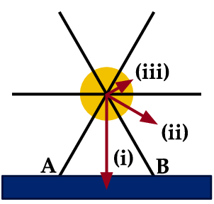
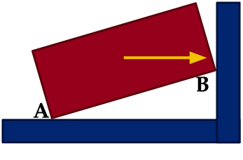
We include, as motivation, two common robotics examples that exhibit simultaneous impacts: one related to legged locomotion and the other to manipulation. Both examples, depending on initial conditions and model properties, can exhibit non-uniqueness. Before describing our model in full detail, we present these examples by considering the outcome of applying Routh’s method to a single contact at a time.

As post-impact velocity is sensitive to the ordering of individual impact resolutions, if we would like to predict as many reasonable post-impact velocities as possible, we must use as relaxed of a notion of impact resolutions as possible. A similar model, without theoretical results or a detailed understanding, was proposed by Posa et al. 2016b where it proved useful for stability analysis of robots undergoing simultaneous impact. We consider a formulation in which at any given instant during the resolution process, the impacts are allowed to concurrently resolve at any relative rate:

1. 1.

   Monotonically increase the normal impulse on each non-separating contact $c$ at rate $\bm{\lambda}_{n,c}\geq 0$ such that

   $$\sum_{c\in C}\bm{\lambda}_{n,c}=\left\lVert\bm{\lambda}_{n,C}\right\rVert_{1}=1\,.$$

   (15)

2. 2.

   Increment the tangential impulse for each frictional contact $c$ at rate $\bm{\lambda}_{t,c}$ such that $\bm{\lambda}_{C}\in\mathrm{FC}_{C}(\bm{v})\,.$

3. 3.

   Terminate when $\bm{v}\not\in\mathcal{P}_{C}$.

We can understand the constraint (15) on $\bm{\lambda}_{C}$ as choosing a net force that comes from a convex combination of the forces that Routh’s method might select for any of the individual contacts $c\in C$. As in the single contact case, we might instead think of the selection of a $\bm{\lambda}_{C}$ as picking an element of a set of admissible values for $\dot{\bm{v}}$. As before, we construct a u.s.c. differential inclusion to capture this behavior:

$$F_{C}\left(\bm{v}\right)=\mathrm{co}\left(\left\{f_{c}:c\in C,f_{c}\in F_{c}(\bm{v}),\bm{v}\in\mathrm{cl}\mathcal{P}_{c}\right\}\right)\,,$$

(16)

$\displaystyle D_{C}(\bm{v})=\begin{cases}\left\{\bm{0}\right\}&\bm{v}\in\mathcal{A}_{C}\,,\\ F_{C}\left(\bm{v}\right)&\bm{v}\in\mathcal{P}_{C}\,,\\ \mathrm{co}\left(\left\{\bm{0}\right\}\cup F_{C}(\bm{v})\right)&\mathrm{otherwise}\,.\end{cases}$

(17)

We denote total impulse over an interval $[s_{1},s_{2}]$, $\bm{\Lambda}_{C}\left(s_{1},s_{2}\right)$, as before. Similar to (13), one can extract $\bm{\lambda}_{C}(s)$ from a solution $\bm{v}(s)$ such that

$$\dot{\bm{v}}=\bm{J}_{C}^{T}\bm{\lambda}_{C},\qquad\left\lVert\bm{\lambda}_{n,C}\right\rVert_{1}=1\,,\qquad\bm{\lambda}_{C}\in\mathrm{FC}_{C}(\bm{q},\bm{v})\,.$$

(18)

We illustrate the behavior of this model on the rimless wheel in Figure 3(b). While $\bm{v}$ remains in the third quadrant, the direction of $\dot{\bm{v}}$ is permitted to take any value in the convex cone outlined by the sold blue and dotted red solutions, including the simultaneous impact solution. This results in the velocity terminating at least one impact on the dashed orange set, after which behavior is identical to the single-contact system. The final velocities achievable, shown in solid green, are a superset of those given by sequential and simultaneous resolution.

The construction of (17) is similar to that of the single contact system (11); it is furthermore equivalent when $C$ is a singleton. We now detail properties of the multi-contact system that are useful for analyzing its solution set.

Let $\bm{R}$ be a matrix with columns that constitute an orthogonal basis of $\mathrm{Range}\left(\bm{J}_{c}^{T}\right)$. By equivalence of norms there exists $\epsilon>0$ such that

$$\left\lVert\bm{J}_{n,c}\bm{v}\right\rVert_{1}+\left\lVert\bm{J}_{t,c}\bm{v}\right\rVert_{2}\geq\epsilon\left\lVert\bm{R}^{T}\bm{v}\right\rVert_{2}.$$

(34)

Pick $S=\left(\epsilon\min\left(\bm{\mu}_{c},1\right)\right)^{-1}$. Let $V(s)=\left\lVert\bm{R}^{T}\bm{v}(s)\right\rVert_{2}^{2}$. Assume $\bm{v}(s)\in\mathcal{P}_{c}$ for $s<s^{*}=\left\lVert\bm{R}^{T}\bm{v}(0)\right\rVert_{2}S\leq\left\lVert\bm{v}(0)\right\rVert_{2}S$.

	$\displaystyle\dot{V}$	$\displaystyle=2\dot{\bm{v}}^{T}\bm{R}\bm{R}^{T}\bm{v}\,,$		(35)
		$\displaystyle\in 2\left(\bm{J}_{n,c}-\bm{\mu}_{c}\mathrm{Unit}\left(\bm{J}_{t,c}\bm{v}\right)^{T}\bm{J}_{t,c}\ \right)\bm{R}\bm{R}^{T}\bm{v}\,,$		(36)
		$\displaystyle=-2\left\lVert\bm{J}_{n,c}\bm{v}\right\rVert_{1}-2\bm{\mu}_{c}\left\lVert\bm{J}_{t,c}\bm{v}\right\rVert_{2}\,,$		(37)
		$\displaystyle\leq-2\epsilon\min\left(\bm{\mu}_{c},1\right)\sqrt{V}\,,$		(38)

on $[0,s^{*}]$ and thus $V\left(s^{*}\right)\leq\left(\sqrt{V(0)}-\epsilon\min\left(\bm{\mu}_{c},1\right)s^{*}\right)^{2}=0$. Therefore $\bm{J}_{n,c}\bm{v}\left(s^{*}\right)=0$.

Let $\bm{v}(s)\in\mathrm{SOL}_{D_{C}}\left(I\right)$ with $\bm{v}(s)$ non-constant. Let $\bm{\lambda}_{C}(s)$ be the associated vector of force variables. As $\bm{v}(s)$ is continuous, we may select $s^{*}\in\mathrm{int}I$ such that $\forall\delta>0$, $\bm{v}(s)$ is non-constant on $[s^{*},s^{*}+\delta]$. Let $A=\left\{a\in S:\bm{J}_{n,a}\bm{v}(s^{*})\leq 0\right\}$ be the set of active contacts at $s=s^{*}$. Let $B$ the the largest subset of $A$ such that $\bm{J}_{n,B}\bm{v}=\bm{0}$ and $\bm{J}_{t,B}\bm{v}=\bm{0}$. As $\bm{v}$ is continuous, $\exists\delta_{\epsilon}>0$ and $\epsilon>0$ such that $\forall s\in[s^{*},s^{*}+\delta_{\epsilon}]\subseteq I$,

• •

  $\bm{J}_{n,C\setminus A}\bm{v}(s)>\epsilon$

• •

  $\bm{J}_{n,c}\bm{v}(s)<-\epsilon$ for $c\in A\setminus B$ frictionless

• •

  $\bm{J}_{n,c}\bm{v}(s)<-\epsilon$ or $\left\lVert\bm{J}_{t,c}\bm{v}(s)\right\rVert_{2}>\frac{1}{\bm{\mu}_{i}}\epsilon$ for $c\in A\setminus B$ frictional.

Therefore no new contacts activate before $s^{*}+\delta_{\epsilon}$, and

$$\bm{v}(s)=\bm{v}(s^{*})+\bm{J}_{C}^{T}\bm{\Lambda}_{C}(s^{*},s)=\bm{v}(s^{*})+\bm{J}_{A}^{T}\bm{\Lambda}_{A}(s^{*},s)\,,$$

(39)

on $[s^{*},s^{*}+\delta_{\epsilon}]$. Select one such $s$ with $\bm{v}(s)\neq\bm{v}(s^{*})$. By Lemma 5,

	$\displaystyle 0$	$\displaystyle\geq\frac{1}{2}\left\lVert\bm{v}(s)\right\rVert_{2}^{2}-\frac{1}{2}\left\lVert\bm{v}(s^{*})\right\rVert_{2}^{2}\,,$		(40)
		$\displaystyle=\bm{v}(s^{*})^{T}\left(\bm{v}(s)-\bm{v}(s^{*})\right)+\frac{1}{2}\left\lVert\bm{v}(s)-\bm{v}(s^{*})\right\rVert_{2}^{2}\,,$		(41)
		$\displaystyle=\left(\bm{J}_{A\setminus B}v(s^{*})\right)^{T}\bm{\Lambda}_{A\setminus B}(s^{*},t)+\frac{1}{2}\left\lVert\bm{v}(s)-\bm{v}(s^{*})\right\rVert_{2}^{2}\,.$		(42)

Therefore, we must have $\left\lVert\bm{\Lambda}_{A\setminus B}(s^{*},t)\right\rVert_{1}>0$. Finally,

	$\displaystyle K(\bm{v}(s))$	$\displaystyle=K(\bm{v}(s^{*}))+\int_{s^{*}}^{s}(\bm{J}_{c}\bm{v}(\tau))^{T}\bm{\lambda}_{c}(\tau)\mathrm{d}\tau\,,$		(43)
		$\displaystyle\leq K(\bm{v}(s^{*}))-\epsilon||\Lambda_{A\setminus S}(s^{*},s)||_{1}\,,$		(44)
		$\displaystyle<K(\bm{v}(s^{*}))\,.$		(45)

Therefore $\left\lVert\bm{v}\right\rVert_{2}$ is non-constant.

References

- Anitescu and Potra [1997] M Anitescu and F A Potra. Formulating dynamic multi-rigid-body contact problems with friction as solvable linear complementarity problems. Nonlinear Dynamics, 14(3):231–247, 1997.
- Aubin and Cellina [1984] Jean-Pierre Aubin and Arrigo Cellina. Differential Inclusions: Set-Valued Maps and Viability Theory (Grundlehren Der Mathematischen Wissenschaften). Springer Verlag, 1984. ISBN 0387131051.
- Bhatt and Koechling [1995] V Bhatt and J Koechling. Three-dimensional frictional rigid-body impact. Journal of Applied Mechanics, 62:893, 1995.
- Brogliato [1999] B Brogliato. Nonsmooth mechanics: models, dynamics, and control. Springer Verlag, 1999.
- Burden et al. [2016] Samuel A. Burden, S. Shankar Sastry, Daniel E. Koditschek, and Shai Revzen. Event–Selected Vector Field Discontinuities Yield Piecewise–Differentiable Flows. SIAM Journal on Applied Dynamical Systems, 15(2):1227–1267, jan 2016. ISSN 1536-0040. doi: 10.1137/15M1016588. URL http://epubs.siam.org/doi/10.1137/15M1016588.
- Chatterjee and Ruina [1998] A Chatterjee and A Ruina. A New Algebraic Rigid-Body Collision Law Based on Impulse Space Considerations. Journal of Applied Mechanics, 65(4):939–951, 1998.
- Chavan-Dafle and Rodriguez [2017] Nikhil Chavan-Dafle and Alberto Rodriguez. Stable Prehensile Pushing: In-Hand Manipulation with Alternating Sticking Contacts. oct 2017. URL http://arxiv.org/abs/1710.11097.
- Coleman et al. [1997] Michael J Coleman, Anindya Chatterjee, and Andy Ruina. Motions of a Rimless Spoked Wheel: a Simple 3D System with Impacts. Dynamics and Stability of Systems, 12(3):139–160, 1997.
- Coumans and Erwin [2015] Erwin Coumans and Erwin. Bullet physics simulation. In ACM SIGGRAPH, page 1, New York, New York, USA, 2015. ACM Press. ISBN 9781450336345. doi: 10.1145/2776880.2792704. URL http://dl.acm.org/citation.cfm?doid=2776880.2792704.
- Drumwright and Shell [2010] Evan Drumwright and Dylan A. Shell. Modeling Contact Friction and Joint Friction in Dynamic Robotic Simulation Using the Principle of Maximum Dissipation. pages 249–266. Springer, Berlin, Heidelberg, 2010. doi: 10.1007/978-3-642-17452-0˙15. URL http://link.springer.com/10.1007/978-3-642-17452-0{_}15.
- Erleben [2004] Kenny Erleben. Stable, Robust, and Versatile Multibody Dynamics Animation. Unpublished Ph. D. Thesis, University of Copenhagen, Copenhagen, 2004. URL http://image.diku.dk/kenny/download/erleben.05.thesis.pdf.
- Fazeli et al. [2017a] Nima Fazeli, Samuel Zapolsky, Evan Drumwright, and Alberto Rodriguez. Learning Data-Efficient Rigid-Body Contact Models: Case Study of Planar Impact. oct 2017a. URL https://arxiv.org/abs/1710.05947.
- Fazeli et al. [2017b] Nima Fazeli, Samuel Zapolsky, Evan Drumwright, and Alberto Rodriguez. Fundamental Limitations in Performance and Interpretability of Common Planar Rigid-Body Contact Models. 2017b. URL https://arxiv.org/pdf/1710.04979.pdf.
- Halm and Posa [2018] Mathew Halm and Michael Posa. A Quasi-static Model and Simulation Approach for Pushing, Grasping, and Jamming. In To appear in the Workshop on the Algorithmic Foundations of Robotics (WAFR), 2018.
- Hogan and Rodriguez [2016] Francois Robert Hogan and Alberto Rodriguez. Feedback Control of the Pusher-Slider System: A Story of Hybrid and Underactuated Contact Dynamics. nov 2016. URL http://arxiv.org/abs/1611.08268.
- Horak and Trinkle [2019] Peter C. Horak and Jeff C. Trinkle. On the Similarities and Differences Among Contact Models in Robot Simulation. IEEE Robotics and Automation Letters, 4(2):493–499, apr 2019. ISSN 2377-3766. doi: 10.1109/LRA.2019.2891085. URL https://ieeexplore.ieee.org/document/8603801/.
- Hurmuzlu and Marghitu [1994] Yildirim Hurmuzlu and Dan B. Marghitu. Rigid Body Collisions of Planar Kinematic Chains With Multiple Contact Points. The International Journal of Robotics Research, 13(1):82–92, feb 1994. ISSN 0278-3649. doi: 10.1177/027836499401300106. URL http://journals.sagepub.com/doi/10.1177/027836499401300106.
- Ivanov [1995] A.P Ivanov. On multiple impact. Journal of Applied Mathematics and Mechanics, 59(6):887–902, jan 1995. ISSN 0021-8928. doi: 10.1016/0021-8928(95)00122-0. URL https://www.sciencedirect.com/science/article/pii/0021892895001220.
- Jia et al. [2013] Yan-Bin Jia, Matthew T Mason, and Michael A Erdmann. Multiple impacts: A state transition diagram approach. The International Journal of Robotics Research, 32(1):84–114, jan 2013. ISSN 0278-3649. doi: 10.1177/0278364912461539. URL http://journals.sagepub.com/doi/10.1177/0278364912461539.
- Jiang and Liu [2018] Yifeng Jiang and C. Karen Liu. Data-Augmented Contact Model for Rigid Body Simulation. mar 2018. URL https://arxiv.org/abs/1803.04019.
- Johnson et al. [2016] Aaron M Johnson, Samuel A Burden, and Daniel E Koditschek. A hybrid systems model for simple manipulation and self-manipulation systems. The International Journal of Robotics Research, 35(11):1354–1392, sep 2016. ISSN 0278-3649. doi: 10.1177/0278364916639380. URL http://journals.sagepub.com/doi/10.1177/0278364916639380.
- Kaufman et al. [2008] Danny M Kaufman, Shinjiro Sueda, Doug L James, and Dinesh K Pai. Staggered projections for frictional contact in multibody systems. In ACM Transactions on Graphics (TOG), volume 27, page 164. ACM, 2008.
- Kemp et al. [2007] Charles Kemp, Aaron Edsinger, and Eduardo Torres-Jara. Challenges for robot manipulation in human environments [Grand Challenges of Robotics]. IEEE Robotics & Automation Magazine, 14(1):20–29, mar 2007. ISSN 1070-9932. doi: 10.1109/MRA.2007.339604. URL http://ieeexplore.ieee.org/document/4141029/.
- Liu et al. [2008] Caishan Liu, Zhen Zhao, and Bernard Brogliato. Frictionless multiple impacts in multibody systems. I. Theoretical framework. Proceedings Of the Royal Society A: Mathematical, Physical, and Engineering Sciences, 464(2100), 2008. doi: 10.1098/rspa.2008.0078. URL https://royalsocietypublishing.org/doi/pdf/10.1098/rspa.2008.0078.
- Mordatch et al. [2015] Igor Mordatch, Kendall Lowrey, and Emanuel Todorov. Ensemble-CIO: Full-body dynamic motion planning that transfers to physical humanoids. In Intelligent Robots and Systems (IROS), 2015 IEEE/RSJ International Conference on, pages 5307–5314. IEEE, 2015.
- Parrilo [2003] P A Parrilo. Semidefinite programming relaxations for semialgebraic problems. Mathematical Programming, 96(2):293–320, 2003.
- Posa et al. [2014] Michael Posa, Cecilia Cantu, and Russ Tedrake. A Direct Method for Trajectory Optimization of Rigid Bodies Through Contact. International Journal of Robotics Research, 33(1):69–81, jan 2014.
- Posa et al. [2016a] Michael Posa, Scott Kuindersma, and Russ Tedrake. Optimization and stabilization of trajectories for constrained dynamical systems. In 2016 IEEE International Conference on Robotics and Automation, volume 2016-June, pages 1366–1373, Stockholm, Sweden, may 2016a. ISBN 9781467380263. doi: 10.1109/ICRA.2016.7487270.
- Posa et al. [2016b] Michael Posa, Mark Tobenkin, and Russ Tedrake. Stability analysis and control of rigid-body systems with impacts and friction. IEEE Transactions on Automatic Control (TAC), 61(6):1423–1437, jun 2016b.
- Remy [2017] C David Remy. Ambiguous collision outcomes and sliding with infinite friction in models of legged systems. The International Journal of Robotics Research, 36(12):1252–1267, oct 2017. ISSN 0278-3649. doi: 10.1177/0278364917731820. URL http://journals.sagepub.com/doi/10.1177/0278364917731820.
- Routh [1891] E J Routh. Dynamics of a system of rigid bodies. MacMillan and co. London, 1891.
- Rudin [1986] Walter Rudin. Real and Complex Analysis. McGraw-Hill Education, 1986. ISBN 0070542341.
- Rudin [1991] Walter Rudin. Functional Analysis. McGraw-Hill Science/Engineering/Math, 1991. ISBN 0070542368.
- Salehian and Billard [2018] Seyed Sina Mirrazavi Salehian and Aude Billard. A Dynamical-System-Based Approach for Controlling Robotic Manipulators During Noncontact/Contact Transitions. IEEE Robotics and Automation Letters, 3(4):2738–2745, oct 2018. ISSN 2377-3766. doi: 10.1109/LRA.2018.2833142. URL https://ieeexplore.ieee.org/document/8354896/.
- Seghete and Murphey [2014] Vlad Seghete and Todd D. Murphey. A Propagative Model of Simultaneous Impact: Existence, Uniqueness, and Design Consequences. IEEE Transactions on Automation Science and Engineering, 11(1):154–168, jan 2014. ISSN 1545-5955. doi: 10.1109/TASE.2013.2267731. URL http://ieeexplore.ieee.org/document/6572900/.
- Smith et al. [2012] Breannan Smith, Danny M. Kaufman, Etienne Vouga, Rasmus Tamstorf, and Eitan Grinspun. Reflections on simultaneous impact. ACM Transactions on Graphics, 31(4):1–12, jul 2012. ISSN 07300301. doi: 10.1145/2185520.2185602. URL http://dl.acm.org/citation.cfm?doid=2185520.2185602.
- Stewart and Trinkle [1996] David Stewart and J. C. Trinkle. An Implicit Time-Stepping Scheme for Rigid Body Dynamics with Coulomb Friction. International Journal for Numerical Methods in Engineering, 39(15):2673—-2691, 1996. URL http://citeseerx.ist.psu.edu/viewdoc/summary?doi=10.1.1.61.1260.
- Stewart [2000] David E. Stewart. Rigid-Body Dynamics with Friction and Impact, volume 42. jan 2000. ISBN 0036144599360. doi: 10.1137/S0036144599360110. URL http://epubs.siam.org/doi/abs/10.1137/S0036144599360110.
- Stronge [1990] W J Stronge. Rigid body collisions with friction. Proceedings of the Royal Society of London. Series A: Mathematical and Physical Sciences, 431(1881):169–181, 1990.
- Tan et al. [2018] Jie Tan, Tingnan Zhang, Erwin Coumans, Atil Iscen, Yunfei Bai, Danijar Hafner, Steven Bohez, and Vincent Vanhoucke. Sim-to-Real: Learning Agile Locomotion For Quadruped Robots. In Robotics: Science and Systems, 2018. URL https://arxiv.org/pdf/1804.10332.pdf.
- Uchida et al. [2015] Thomas K Uchida, Michael A Sherman, and Scott L Delp. Making a meaningful impact: modelling simultaneous frictional collisions in spatial multibody systems. Proceedings of the Royal Society of London A: Mathematical, Physical and Engineering Sciences, 471(2177):20140859–20140859, 2015. ISSN 1364-5021. doi: 10.1098/rspa.2014.0859. URL http://rspa.royalsocietypublishing.org/content/471/2177/20140859.abstract.
- Wang et al. [1992] Y.-T. Wang, V. Kumar, and J. Abel. Dynamics of rigid bodies undergoing multiple frictional contacts. In Proceedings 1992 IEEE International Conference on Robotics and Automation, pages 2764–2769. IEEE Comput. Soc. Press, 1992. ISBN 0-8186-2720-4. doi: 10.1109/ROBOT.1992.220016. URL http://ieeexplore.ieee.org/document/220016/.
- Wieber et al. [2016] Pierre-Brice Wieber, Russ Tedrake, and Scott Kuindersma. Modeling and Control of Legged Robots. In Springer Handbook of Robotics, pages 1203–1234. Springer International Publishing, Cham, 2016. doi: 10.1007/978-3-319-32552-1˙48. URL http://link.springer.com/10.1007/978-3-319-32552-1{_}48.