Fault tolerant resource estimation of quantum random-access memories
Abstract
Quantum random-access look-up of a string of classical bits is a necessary ingredient in several important quantum algorithms. In some cases, the cost of such quantum random-access memory (qRAM) is the limiting factor in the implementation of the algorithm. In this paper we study the cost of fault-tolerantly implementing a qRAM. We construct and analyze generic families of circuits that function as a qRAM, discuss opportunities for qubit-time tradeoffs, and estimate their resource costs when embedded in a surface code.
I Introduction
Random-access memory (RAM) is an essential component of classical computing architectures. Many quantum algorithms require an analogous system, a so-called quantum RAM, or qRAM, where the input is a quantum state, the routing components are inherently quantum, and the information stored can be either classical, i.e. or , or quantum, i.e. any arbitrary superposition of and . In the present paper we consider qRAM that stores only classical information. Generically, such a memory allows for the querying of a superposition of addresses
| (1) |
where is a superposition of queried addresses and represents the content of the -th memory location. A memory that stores classical information but allows queries in superposition is required for quantum algorithms such as Grover’s search on a classical database PhysRevLett.79.325, collision finding Brassard:1997:QCH:261342.261346, element distinctness Ambainis:2007:QWA:1328722.1328730, dihedral hidden subgroup problem Kuperberg:2005:SQA:1085579.1093661, phase estimation for electronic structure simulation Babbush2018, and various practical applications mentioned in arunachalam2014quantum. In fact, such a quantum memory often plays the role of the oracle and is ideal in implementing any oracle-based quantum algorithm, in which the oracle is used to query classical data in superposition.
Several authors described algorithms that require only a polynomial amount of resources such as computational qubits or depth, and some larger number of ‘quantumly accessible’ classical bits 10.1007/978-3-642-38616-9_6. Such quantumly accessible classical bits are less costly for classical simulations of quantum computers, since a quantum algorithm with qubits and qRAM bits can be simulated with classical bits, instead of .
There are also numerous algorithms, for example in quantum machine learning and Hamiltonian simulation, that are shown to demonstrate a speedup but must assume a qRAM can be queried efficiently (for example, Kerenidis2016; Wang2018; Zhao2018). For many algorithms this dependence stems from using the HHL algorithm for solving linear systems as a subroutine HHL, which itself is successful in practice assuming we can query efficiently, though we note that the particular operation performed by the qRAM differs slightly from the one we analyze here 11 1 In contrast to Equation (1), the data to be read in is a vector of complex numbers which become the amplitudes in a superposition, e.g. . .
One qRAM implementation, the bucket brigade method Giovannetti2008, may allow algorithms that make only a few queries to a qRAM to avoid the usual overhead associated with fault-tolerant implementation of a binary-tree type look-up circuit. For such few-query algorithms this may bring substantial savings. However for many-query algorithms, it does not appear that one can bypass fault-tolerant error correction Arunachalam2015. It remains unclear whether there is in fact much of a savings over general purpose quantum memory when implementing a fault-tolerant qRAM for a quantum computation.
Our work here seeks to address the question of the cost of fault-tolerant qRAM in a quantum computation. This cost is comprised of a number of different factors. The primary one we consider here is the execution of a quantum circuit which performs the query, completely embedded in a fault-tolerant error correction scheme. One must also take into account external factors that may stem from the specific physical implementation and/or algorithm which is querying the qRAM. In principle, we can “boot up” our qRAM qubits only when we need to make a query, and turn them off after the fact. However, a combination of the overhead cost of initializing the qubits, cost of resetting them to , as well as any idle time between queries may warrant a more active approach to error correction so that after initialization the qRAM remains perpetually on (in a sense this would be similar to how conventional RAMs refresh themselves).
Roughly speaking, there are two natural ways to implement a quantum query to a classical memory. At one extreme, classical information could be explicitly laid out in static physical hardware which is quantumly queried. This can be accomplished using, for example, controlled-NOT (CNOT) gates on some target register conditioned on the values of the , or by some binary tree circuit or a bucket brigade-style circuit, which has depth logarithmic in the size of the database. Such approaches require a number of query qubits that is proportional to the size of the database. By query qubits, we are referring to the qubits used in essentially all such memory schemes in order to connect the computational qubits that store the index that needs to be queried, and the (qu)bits that store the classical information being queried. These query qubits (or qudits) are only used ephemerally in order to perform the query, and do not store any information before or after each query.
Such an ‘explicit’ qRAM has the advantage that a circuit implementing it needs to be compiled and optimized only once, while the contents of the memory are free to change. The disadvantage is the significant space overhead required, since we need as many qubits as we have bits in the database, and these qubits need to be initialized and maintain coherence.
At the other extreme, instead of storing the classical information in a static physical memory, one can simply implement a sequence of mixed-polarity multi-controlled CNOTs conditioned on the control bits representing the memory address of a 1 22 2 Of course, if there are more 1s than 0s, it suffices to condition instead on the control bits representing the memory addresses of the 0s and then finish with a single NOT gate. Later in the paper we discuss other optimizations that can be performed based on structure or patterns in the data.. This implies that the classical database is implicitly stored in the logical circuit, and this circuit will have depth proportional to the number of 1s in the database.
An advantage of ‘implicit’ circuits is that they can be heavily optimized using any number of known optimization techniques for Boolean circuits. However, an implicit qRAM requires us to know the contents of the memory in advance. Writing to the qRAM consists of the addition or removal of a multi-controlled CNOT corresponding to the desired address, meaning that any change in the database would require recompilation and optimization of the circuit.
We present variants of this latter approach that only require resources roughly proportional to the number of 1s in the database. Suppose there are 1s in the database. We can perform a sequence of multiple controlled gates, where each address containing a is used to control the output of some target bit. We can also parallelize this process: in depth we can compute copies of the desired index. Then in parallel, using the -th copy of the desired index we compute if the index equals the index of the th 1 in the database. Finally, using a binary tree type circuit we can in depth compute whether a was computed on any of the copies. We then uncompute all the intermediate computations.
There are also many natural ways to interpolate between the two approaches, for example using the same fan-out like operation to make copies of the first index bits, and then use parallel logical circuits to explore the remaining index bits.
In this paper, we outline these various questions and approaches, and consider their costs and trade-offs. Such an analysis is important for optimizing the physical resources needed to implement in practice quantum algorithms that use a qRAM repeatedly, using the best-known methods. We begin by describing our general cost model and how we presume an algorithm will query the qRAM. We then introduce a number of circuit families: circuits for the bucket brigade qRAM model, the basic highly sequential or parallel circuits mentioned above, as well as some interpolations between the two. Under assumptions about our physical parameters and our database, we will compute concrete parameters such as real-time cost, number of qubits, etc. of our circuits embedded within a fault tolerant implementation using a defect-based surface code Fowler2012. Following this, we apply our techniques to a family of circuits recently designed by other researchers Vadym2018, demonstrating how targeted optimization can significantly reduce the resources costs. We conclude with some final thoughts and present avenues for future research. Finally, we note that we have made available a code repository including our data as well as circuit details and resource estimation procedures code.
II Modeling the cost of a qRAM
We consider a qRAM that stores quantumly accessible classical bits. Locations in memory are addressed by -bit strings , and are queried by inputting the associated state to a circuit. The memory contents may be stored explicitly in additional qubits which are coupled to during the query, or implicitly in the circuit given prior knowledge of the database. In both models, for each address the qRAM should implement
| (2) |
where is the stored value at the specified address. This form ensures the qRAM can be queried in superposition.
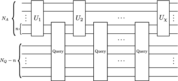
Consider a quantum algorithm with a structure similar to that in Figure 1. Queries to a qRAM are interspersed between some number of arbitrary unitary operations that comprise the main portion of the algorithm. We suppose that the entire circuit is embedded in a surface code in order to make it fault-tolerant. Then, we can use the same cost metric as SHAPaper, wherein
| (3) |
In essence this cost represents a tradeoff of space vs. time.
The cost is calculated using a framework SHAPaper that starts from the high-level algorithmic description. The algorithm begets a quantum circuit, which is then synthesized and optimized over an elementary gate set (we use Clifford+). The optimized circuit is then embedded into a surface code, in which the number of logical qubits and operations determine parameters such as code distance and resources required for magic state distillation. With these, we can compute physical layer parameters such as the number of physical qubits and surface code cycles.
In the present work we will take a more general approach to calculating cost. We will compute the cost of an ‘isolated’ qRAM circuit making a large number of queries and express it in terms of parameters such as , and the number of 1s stored in the memory. We will not be dealing with any specific algorithms or circuits. As a consequence, we cannot perform the kind of extensive optimization that may be afforded to us when we know the memory contents. We can, however, consider higher-level optimizations, such as the choice of decomposition of the mixed-polarity gates.
We will also use a ‘rough’ estimate of cost before performing the surface code analysis:
| (4) |
gates are the most expensive part of the implementation due to the need to distill magic states, and the algorithm will be time-limited to how quickly we can produce these states. Magic states are distilled in separate surface codes called distilleries; once a state has been distilled, it can be held in reserve and injected into the circuit when needed Fowler2012. In the interest of minimizing time, it is beneficial to have multiple distilleries running simultaneously, especially since in many of our circuits we will need to run gates in parallel. However, adding distilleries incurs an additional cost due to the increased number of physical qubits. One must therefore choose this quantity based on the available resources.
In our analysis we select the number of distilleries by considering the average -width , where is the total -count of the algorithm, and is the -depth, i.e. the number of layers of depth that contain or gates. In many of the circuits we present, we use repeated copies of sub-circuits (e.g. a Toffoli) which have been pre-optimized such that they have , or close to 1. Then the number of gates in each layer of -depth should be roughly the same, and we will make efficient use of our factories as we will essentially be consuming the required magic states immediately upon creation, using the minimal number of physical qubits required to do so.
III Should I try turning it off and on again?
One question posed in the Introduction was whether or not we should keep the qRAM “on” between queries. By this, we mean performing active error correction on the idle qubits in the qRAM while the algorithmic components run. We will consider this question in terms of the difference in cost of both approaches.
For simplicity, let us assume that the algorithm performs instances of the same operation on qubits, and queries to the qRAM in between these operations, using qubits, as is depicted in Figure 1. As we alternate between queries and operations, the logical qubits in the algorithm (minus the used as an address for the query) will be in an idle state while we query the qRAM; similarly, if we keep the qRAM on, the query qubits will be idle while the algorithmic portions run.
Let be the number of surface code cycles taken by one instance of . We assume that cycles are required for the initialization of a logical qubit, using for example the procedures outlined in Fowler2012. We assume as well that it takes cycles to reset and dispose of the qubits once the query is complete. In a sense, these operations are analogous to C memory management functions calloc() and free() KR:1988:C.
It is straightforward, from Figure 1, to see that we should take the following approach:
Note, however, that since cost involves multiplication by the number of logical qubits, performing any sort of cost analysis on a qRAM is naturally most important when . The choice of query circuit, various options for which will be discussed in the ensuing sections, may thus depend on a tradeoff between available resources and the relative size of the algorithm circuit versus that of the qRAM.
One can also imagine situations in more complex algorithms where the operations are not identical. Here one might design a smart compiler that will choose to periodically turn off the qRAM during comparatively long algorithm operations, but leave it on for shorter ones. A smart compiler may also take into consideration the relative error rates between, say, re-initializing a qubit in versus keeping its existing state error-corrected. This alone may warrant always turning off the qRAM, if can be initialized quickly and with very high accuracy.
Finally, we note that if an algorithm requires writing regular updates to the classical database (such as in 10.1007/978-3-642-38616-9_6), then one would need to update the query circuit during the course of the algorithm. Thus any latency between changing the database based on a measurement during the execution of the quantum circuit and updating the circuit in the software must be considered. Latency would also exist for any other mechanism for storing the database, and the precise cost for each approach would need to be considered in each case.
IV Bucket brigade circuits
The first family of circuits we will analyze are a family introduced in Arunachalam2015 that implement a bucket brigade qRAM Giovannetti2008; Giovannetti2008b. One such circuit is shown in Figure 2. These circuits assume that the contents of the memory are stored statically in the lower register of qubits in Figure 2, in contrast to the circuits we will see in later sections. They are thus not perfectly comparable, however it is of interest nonetheless to estimate the resources required when a bucket-brigade circuit is implemented fault-tolerantly in order to deal with errors when making a large number of queries.
Bucket brigade circuits are constructed using only CNOTs, and Toffolis, which we will further decompose over the Clifford+ gate set. We will perform a cost estimate for two types of bucket brigade circuit, those constructed exactly as in Figure 2, as well as an improved version where we parallelize the execution of the Toffolis in each layer.

We can choose from a number of different implementations of a Toffoli Selinger2013; Amy2014, which will affect the overall resource counts:
- •
No ancillae, -depth 3,
- •
One ancilla, -depth 2,
- •
Four ancillae, -depth 1.
Note that in all cases the ancillae can be reused whenever Toffolis are applied sequentially. We focus on the third option, which while it uses the most ancillae, a simple analysis using the cost function in Equation (4) found this to always produce the lowest cost due to the savings in -depth.
To perform our resource estimates, we assume that the Toffolis in Figure 2 are all implemented using the decomposition in Fig. 1 of Selinger2013, which has -count 7, -depth 1, 16 CNOTs, and depth 7. For a fully reversible qRAM query, we must run the circuit in Figure 2, and then uncompute the fanout of the address bits. For memories with -bit addresses, a bucket brigade circuit thus requires Toffoli gates. This yields resource counts:
| (5) | |||||
We note here that this is only one possible implementation of the bucket brigade scheme, and it is not necessarily the cheapest. If the main algorithm querying the qRAM is concerned with phases (such as in Grover’s algorithm), it would be best to directly implement the phase-shift version of the qRAM, i.e. . We could accomplish this by replacing the final sequence of Toffolis with controlled-phase gates from each address fanout qubit down to the corresponding memory location. This would significantly reduce the circuit depth and -depth in the circuit of Figure 2, and also eliminate the need for the final output qubit. 33 3 Conversely, it is known how to convert phase-shift queries to bit-flip queries at the logical level as well, though with a small overhead. In a concrete application, the subtle cost differences between the two approaches should be evaluated to decide whether overall a phase-flip qRAM or bit-flip qRAM is more efficient. For this paper, we focus on the slightly harder bit-flip look-up.
We naturally can also parallelize this circuit by a) copying down the address qubits to ancillae so that the Toffolis in the address fanout layers can be performed in parallel, and b) adding an extra output register of qubits in the superposition of all even-parity states to collect the results of the final set of Toffolis, followed by CNOTs to compute the parity (as is depicted later in Figure 4). We then copy down to an output bit, apply another CNOT back to the even-superposition register, and then uncompute the parity as well as the address bit fanout.
We need to prepare the even-parity superposition only once at the beginning, and uncompute it at the end, as by design this register will remain in superposition after each query. We thus neglect the resources for this procedure in our analysis, as it can be performed in logarithmic depth and becomes negligible for large .
We require enough ancillae to perform the largest amount of simultaneous Toffolis, which will be using the -depth 1 implementation. While in absolute terms this adds an exponential number of qubits, it will yield a significant savings in -depth and, we will see, reduce the overall cost.
For computing the circuit depth, note that computation of parity in the output register can be done at the same time as uncomputation of the address fanout portion, so it does not contribute to the depth. Furthermore, the initial copying of the address bits (so that the fanout Toffolis can be run in parallel) requires in the worst case layers of depth, all of which can be absorbed in the calculation of the preceding Toffolis. Thus, the depth of the fanout portion is simply the depth of Toffolis, plus for the initial CNOTs and layers in between the Toffolis.
Putting together the resource counts for the entire circuit, we obtain:
| (6) | |||||
The rough cost scaling of in terms of is greatly improved in the parallelized circuit, and so moving forward we will consider only the parallel version.
V Basic query circuits
We now construct families of ‘implicit’ qRAM circuits that will highlight the space-time tradeoff required for a fault-tolerant qRAM. We will see in the end that they have comparable overall cost, but vastly differing use of resources down at the physical level.
For these circuits, we suppose for simplicity that the memory contains 1s, the locations of which are known, with the rest being 0. Note that this is in contrast to the bucket brigade circuits where the contents, while unknown, were provided to us statically stored in hardware. Recall that if the number of 1s is ever greater than the number of 0s, we can equally well build our circuits by inputting the locations of the 0s.
We consider a small running example for the purpose of creating the circuit diagrams. Suppose we have and , i.e. 4 of 8 memory locations store a 1. We arbitrarily set those locations to be 000, 001, 011, 111.
V.1 Large depth, small width circuit
We can easily create a circuit that outputs 1 for the valid addresses by implementing a sequence of -bit mixed-polarity multiple control Toffolis (MPMCTs). The circuit for the running example is shown in Figure 3. Each MPMCT is tied to one of the addresses, and sets a target bit to 1 only if its associated address is fed in. Henceforth we assume that we have a random database where we don’t know the exact sequence of MPMCTs, only that we have such operations. As such, we will not perform any extensive circuit optimization in our analysis, and will focus on this worst case.

In general, when a sequence of MPMCTs is known, we may be able to greatly simplify the circuit. For example, since a sequence of MPMCTs represents a Boolean function which is a sum of product terms, we can find its ESOP expression using a tool such as EXORCISM-4 Mishchenko2001. This can offer great savings - for example, the circuit in our example can be reduced to 2 Toffolis just by factoring some terms in the Boolean expression. We can also use the method of Shafaei2013 which first computes the ESOP, and then breaks the expression down into common cofactors of the expression terms; cofactors are then reversibly synthesized individually before being used in their constituent terms.
In our worst-case analysis, we begin instead by performing quantum circuit synthesis to decompose the circuit down into the 1- and 2-qubit operations of the Clifford+ gate set. Again, when the precise sequence of MPMCTs is known, further optimization can be done to reduce parameters such as the -count and -depth (see, for example, the methods in Amy2014).
The decomposition we choose for the MPMCTs is that in Fig. 4 of Abdessaied2016a, which is an optimization of an older algorithm from Barenco1995 that performs an -controlled NOT using ancillae by turning it into a cascade of Toffoli gates. We take advantage of an additional optimization which, at the cost of one more ancilla qubit, can further parallelize some of the gates in the constituent controlled-phase gates (see (9) in Selinger2013). While it may be possible to implement such gates with fewer ancilla qubits, recall that we are interested in plugging this circuit into the surface code, wherein minimization of -count and -depth plays a critical role in reducing the overall cost incurred by magic state distillation. Finally, we note that this MPMCT implementation is valid only for , and so we will limit our analysis to this case.
Using the constructions of Abdessaied2016a and Selinger2013, we calculate the resources required for an -controlled MPMCT gate:
| (7) | |||||
where is the number of Hadamard gates.
We see immediately that in theory, the circuit in Figure 3 requires only qubits, plus ancilla qubits. As the ancillae are returned to their initial state after each MPMCT, we can reuse them for all gates. We note that any gates to change polarity of the controls can be applied in the first layer of depth of each MPMCT; in addition, the final polarity change can be performed in the last layer of the last MPMCT. In all cases the gates do not contribute to depth, and as they are not critical to the overall cost in a fault-tolerant setting, we will disregard them. Thus we obtain total logical resource counts
| (8) | |||||
V.2 Small depth, large width circuit
In contrast to the circuit of the previous section that performs all the MPMCTs sequentially, here we present an implementation that parallelizes their execution. The circuit for our running example is shown in Figure 4.

We begin with registers of qubits, one for each address containing a 1. The address is input to the first register of qubits and then copied down to the others using a log-depth cascade of CNOTs. Each register performs an MPMCT which triggers one of the qubits in an additional register of qubits if the input address matches. This register is prepared in a superposition over even-parity states, as proposed in Section IV. We then compute the parity, copy it to an additional qubit, copy back, and then uncompute parity and the address fanout. We again neglect the resources required to prepare the even-parity superposition, as this need only be done once when performing multiple queries.
The number of qubits, including required ancillae, is
| (9) | |||||
To compute the depth of this circuit, we must take into account the sequences of CNOTs. The initial copying is performed in depth , the parity in depth , plus 2 for copying to the output qubit. As uncomputation of the address fanout has the same depth as parity, we can perform them simultaneously. Thus the depth is
| (10) | |||||
which scales linearly in both and .
The -count will be the same as for the circuit in the previous section, however the -depth will now be as all the MPMCTs are performed in parallel.
In addition, we will need the Clifford counts. The number of Hadamards is unchanged (neglecting the construction of the even-parity superposition). The number of CNOTs in the initial fanout plus a parity computation is
| (11) | |||||
Doubling this, adding 2 for the copying to the output, plus the CNOTs in the MPMCTs, we obtain
| (12) | |||||
In summary, the resources required are
| (13) | |||||
V.3 Preliminary cost estimate
Recall that our definition of cost is a product of space and time. We can analyze to get a rough first estimate of how the cost will depend on and . In Figure 5 we plot the overall costs (including constant prefactors) for differing values of , and for the circuits in which it is relevant. We summarize our observations in Table 1 to make it easier to see the tradeoff between the number of qubits and the depth for each circuit.
| Circuit | Large depth | Large width | Bucket brigade parallel |
|---|---|---|---|
| Cost |


The top panel of Figure 5 shows the situation of a half-full memory in which . This represents a roughly random database, and is the worst case because as mentioned previously, if the memory is more than half-full with 1s, we can switch the polarities of the gates to pick out the locations that are 0 instead.
For a half-full memory, the parallel bucket brigade circuit is the best choice, as it always has lower cost. For memories that are emptier, there is a cross-over point at , before which it is in fact better to use either the large depth or large width circuit as opposed to the bucket brigade circuit (assuming, of course, that one has knowledge or control over the location of the 1s in the memory).
V.4 Surface code analysis
We now embed these circuits into a surface code using the same procedure as in SHAPaper. The implementation, as well as the data, can be found in our code repository code. The (optimistic) surface code parameters are input injection error probability , gate error probability of , and a cycle time of ns.
Figure 6plots the numerical equivalent of Figure 5. While the relative relationships remain the same, the overall cost is significantly higher due to the large amount of logical qubits needed in the distillation factories.
Figure 7is perhaps the more interesting plot, as it shows the explicit tradeoffs between the number of physical qubits and the ‘real’ query time. Even though we observed on Figure 5 that the costs of the large depth/width circuits are comparable, Figure 7 shows us exactly how large the space vs. time tradeoff is.
We present numerical data for the largest and smallest values of we chose, and , in Table 2. The case corresponds to 8 ‘GB’ of classical data in the memory, whereas corresponds to 4 ‘KB’. These particular choices are somewhat meaningful: 4KB was the amount of RAM that the Apple I computer shipped with back in 1976, while 8GB is a fairly standard amount of RAM on a laptop at the time of writing.

| Circuit | Total time (s) | Physical qubits | ||
|---|---|---|---|---|
| Bucket brigade parallel | 15 | - | ||
| Large width small depth | 15 | 14 | ||
| Small width large depth | 15 | 14 | ||
| Bucket brigade parallel | 36 | - | ||
| Large width small depth | 36 | 35 | ||
| Small width large depth | 36 | 35 |
Our analysis shows that quantumly querying the 4KB qRAM can be done with nearly 100 million qubits in roughly 0.35ms (with parallel bucket brigade), or with roughly 42000 qubits in around seconds (small width large depth), however the latter can only be used in cases where we know where the 1s in our memory are. As a reference point, modern-day RAMs have query times on the order of 10-20ns. To query this fast would first of all require significant advances in operational speed (recall our estimate of surface code cycle time was an ambitious 200ns), as well as an astronomical amount of qubits.
Recall also that these numbers have been computed under the assumption that we have as many factories as are needed to implement a single layer of -depth. As all the MPMCTs are the same size, and since they stack in the parallel version, here the -width is an accurate representation of the number of s in each layer. One could, however, adjust the number of factories according to available resources, and the number of physical qubits (time) would decrease (increase) proportionally.

VI Hybrid query circuits
We now investigate a compromise between the two circuits in Section V by creating a sort of hybrid of the two extremes. Our motivation is to explore a wide range of options for the tradeoff between memory and depth to enable an algorithm designer to choose a qRAM implementation based on available resources.
We will need a larger running example: suppose our addresses are now 5 bits, and that addresses 00000, 01001, 10010, 11011, 00100, 01101, 10110, 11111 all contain the value 1 ( full addresses, ).
VI.1 Circuit design
The idea behind the hybrid circuit is, rather than checking the validity of all bits of the address, check only the first , and then use those outputs as controls for checking the rest of the bits. For brevity of analysis we will show here only the case where . Full details for the case can be found in the accompanying code code. We also assume , as recall the MPMCT implementations must have at least 4 control bits.

The circuit for our running example is shown in Figure 8. In the worst case, every possible -bit string occurs as the first bits of at least one address in the space. Thus our top ‘tier’ consists of at most -controlled MPMCTs, and as a consequence, we need at most extra qubits to store their results. The bottom tier will always consist of -controlled MPMCTs, some of which will share the same control bit from the first tier output (in the worst case, this will be of them, as this requires more layers of fanout when we parallelize). Again, in specific cases we could compute the ESOP of the Boolean expressions to simplify the products of MPMCTs, but here we assume them to be unknown.
We continue using the decomposition of the MPMCTs in the previous section. The number of ancillae now depends on the size of vs. - we will need enough ancillae to implement the larger of the two gates. As the ancillae are returned to their initial state after use, we can use the same ancillae for all the gates in the sequence. Finally, to make the query fully reversible, we need to run the top ‘tier’ a second time to return the register of qubits to 0.
We can use the results of the previous sections to compute
| (14) | |||||
We can, in addition, parallelize the hybrid circuit in the same way that we parallelized the original deep circuit. There are three ways to do this: parallelize only the first tier (as shown in Figure 9), parallelize only the second tier, or parallelize both tiers. Parallelizing both tiers is clearly the best choice, as not fully parallelizing will incur additional cost (more qubits) without seeing the full benefit in terms of time saved. We include these other approaches only as an intermediate step and plot them to show how they are sub-optimal. Resource counts for the aforementioned parallelizations can be found in the code.

VI.2 Surface code analysis
We now study the tradeoffs between , , and our new parameter . We will again perform this in two ways, using , as well as a full surface code analysis. The former is plotted in Figure 10, while the surface code results are shown in Figure 11 for a fixed and two different values of .
Unlike in the previous section where the dependence on and could be expressed simply as , the hybrid circuits carry a very complex, intertwined connection between , and . In particular, while we only ever see up to a quadratic dependence on , we see many terms with exponential dependence on and , such as , , etc. For the most part, Figure 10 shows a clear cut exponential dependence on when and are fixed, deviating only at the extremal choices of .
We observe that here in the worst case, when no circuit optimization is performed, the cost of the basic hybrid circuit is actually worse than the simple large depth/width design. Even though the size of the MPMCTs is smaller, there are more of them, and there is the additional exponential increase in the number of logical qubits required to store the outputs of the first tier ( of them). Similarly, parallelizing only a single tier is detrimental to the overall cost. As anticipated, the time saved in parallelizing only one part does not compensate for the substantial increase in the number of qubits required to do so.

Where we do observe an improvement is with the fully parallelized hybrid circuit. In fact the cost of this circuit actually decreases when is increased, and reaches a minimum that we can solve for. For purposes of example, setting , we differentiate the product (full cost expressions can be found in the code, and we look in the limit of based on the graph, and due to the complexity of the expressions). Using as the maximum amount of ancillae yields , which corresponds to the minimum seen in Figure 10 around .
We attribute the decrease in cost with increasing , seen in Figure 10 and Figure 11, to more efficient use of ancillae. When all the MPMCTs are performed in parallel, we need enough ancillae to perform the larger of the two tiers, either for the first tier, or for the second. Recall that we are considering here the case when . When is small and is large, we need a large number of ancillae to perform the second tier, but not many of these need to be reused when performing the first tier. On the other hand as increases and decreases, the number of ancillae needed for the second tier decreases, and furthermore a greater proportion of these can also be used for the first tier. Eventually, we see an increase again as the number needed for the first tier surpasses that of the second. The specific location of this increase depends on the relative values of , and . In the case where , it can be approximated by , which fits with the observed minimum.


Figure 12shows again the tradeoff between physical qubits and time for the hybrid circuits. For our 8GB case, to obtain millisecond-order query times we must still use on the order of physical qubits in the fully parallel version, while a million physical qubits in the basic version yields query times on the order of 3 years.


VII Improving bounds with optimization
The basic circuits of Section V showcase the extremes. Without optimization, these circuits, and even the improved hybrids in Section VI, take a prohibitive amount of resources to execute given the present state of hardware. Taking advantage of special structure and optimization is therefore a critical step moving forward, and work along these lines has already begun to be developed Babbush2018; Childs2018; Vadym2018. Here we analyze one such case Vadym2018 that naturally incorporates tradeoffs in space and time similar to the ones we have explored.
Recall that Figure 1 depicts an algorithm that may use some of its constituent qubits to query a qRAM while the rest remain idle. In a situation where qubits are a limited resource, it would of course be advantageous to use these idle qubits for the query. Such a family of circuits with this property was recently proposed in Vadym2018. Called SelectSwap circuits, they are based on an improved method of performing a uniformly controlled rotation Childs2018, i.e. a sequence of mixed-polarity gates which includes all possible configurations of the control bits, coupled with a network of SWAP gates. While they too depend on knowledge of the database, clearer bounds for their execution can be derived.

An example SelectSwap circuit is shown in Figure 13, as presented in Vadym2018. The circuit consists of two parts, a Select operation where a series of MPMCTs marks the data at the queried address, and a Swap operation that moves the results to an output register. A tradeoff is made using a parameter , which plays a role analogous to the of our hybrid circuits. In a SelectSwap circuit, represents a number of copies to make of an output register to receive the results of MPMCTs. A larger leads to a larger number of qubits, however it also decreases the size and thus resource count of the MPMCTs. In addition to the version of Figure 13, which requires the output registers all be initialized to , it is possible to use dirty ancillae as the input, at the cost of needed to perform the inverse of the SelectSwap operation and a sequence of additional SWAPs.
| Clean anc. | Dirty anc. | |
|---|---|---|
| Qubits | ||
| -depth, | ||
| -count, |
The required resources for both versions are displayed in Table 3. There is a clear improvement in scaling over the hybrid circuits, though we note that only the overall complexity is presented and not explicit resource counts; to make a proper comparison with our circuits would require knowledge of the coefficients and any higher-order terms. Figure 14 shows the qubit and time requirements for the case where and is chosen to be optimal at . The optimal point is clearly visible. In the case of the dirty qubits, the execution time is slightly greater, however this may be a small compromise if we are able to make heavy use of dirty qubits in the rest of the algorithm.

While such analysis shows improvement at the logical level, it is not clear such savings will fully translate to the fault-tolerant level. For example, if the query circuit and algorithm circuit are embedded in different error correcting codes, it might not be possible, or worthwhile to translate between the two in order to use the algorithms dirty qubits.
VIII Conclusion
We have presented a number of different circuit families that perform the task of a qRAM. It is important to note that our resource estimates are based on the worst-case situations of each. One should always, of course, do what’s best for the problem at hand. For a specific algorithm, application of circuit synthesis and optimization techniques may yield lower cost for, e.g. one of the partially-parallelized hybrid circuits rather than the fully-parallelized versions.
Regardless, we can still draw some interesting conclusions from our analysis. First, unsurprisingly, to implement a fault-tolerant qRAM with as much logical memory as a current-generation laptop is infeasible under our physical assumptions and the current state of quantum hardware and quantum fault-tolerant error correction. Under our (currently optimistic) assumptions and using current fault-tolerant quantum error correction, an 8GB qRAM that is roughly half-full uses quadrillions of qubits to obtain fast query times on the order of milliseconds; alternatively, working with only millions of physical qubits would yield query times on the order of years. While circuit optimization may alleviate this to some degree, except for cases with non-trivial structure, we do not anticipate this will shave off enough orders of magnitude to make a fault-tolerant circuit-based qRAM of this size feasible in the foreseeable future.
We also note that while our main analysis assumes generic unstructured data, substantial optimizations are possible when there is special structure in the data. For example, if bit , is known to be a function of bits , where , then depending on the complexity of computing from the relevant values of , it may be most efficient to build a qRAM for the values and compute the values in the circuit making the queries. A particular example, discussed in DiMatteo2018 and included in our software, is the case where the address space has Cartesian product structure. We can take advantage of this to write a circuit that queries two smaller qRAMs and then check the validity of both parts using a Toffoli gate. Finding such structures that are useful in practical is an interesting area for future work.
One significant opportunity for improvement is in the implementation of the surface code. Lattice surgery has recently been shown to yield a decrease in resource estimates, in some cases lowering the number of physical qubits by a factor of 4 to 5 Horsman2011; Litinski2018; Fowler2018. While a factor of 5 may not have much of an effect on circuits requiring quadrillions of qubits, it is promising for smaller qRAMs requiring on the order of 10000 qubits. Further improvements in fault-tolerant methods as well as advances in experimental techniques for reducing physical error rates may make small qRAMs feasible in the nearer term.
Acknowledgments
We thank Matthew Amy, Austin Fowler, Craig Gidney, Alexandru Paler, and Mathias Soeken for useful discussions. We also thank Dominic Berry and Craig Gidney for directing us to reference Vadym2018. We acknowledge support from NSERC and CIFAR. IQC and the Perimeter Institute are supported in part by the Government of Canada and the Province of Ontario.
References
- [1] Lov K. Grover. Quantum mechanics helps in searching for a needle in a haystack. Phys. Rev. Lett., 79:325–328, Jul 1997.
- [2] Gilles Brassard, Peter Høyer, and Alain Tapp. Quantum cryptanalysis of hash and claw-free functions. SIGACT News, 28(2):14–19, June 1997.
- [3] Andris Ambainis. Quantum walk algorithm for element distinctness. SIAM J. Comput., 37(1):210–239, April 2007.
- [4] Greg Kuperberg. A subexponential-time quantum algorithm for the dihedral hidden subgroup problem. SIAM J. Comput., 35(1):170–188, July 2005.
- [5] Ryan Babbush, Craig Gidney, Dominic W. Berry, Nathan Wiebe, Jarrod McClean, Alexandru Paler, Austin Fowler, and Hartmut Neven. Encoding Electronic Spectra in Quantum Circuits with Linear T Complexity. arXiv:1805.03662 [cond-mat, physics:physics, physics:quant-ph], May 2018. arXiv: 1805.03662.
- [6] Srinivasan Arunachalam. Quantum speed-ups for boolean satisfiability and derivative-free optimization. Master’s Thesis, University of Waterloo, 2014.
- [7] Thijs Laarhoven, Michele Mosca, and Joop van de Pol. Solving the shortest vector problem in lattices faster using quantum search. In Philippe Gaborit, editor, Post-Quantum Cryptography, pages 83–101, Berlin, Heidelberg, 2013. Springer Berlin Heidelberg.
- [8] I. Kerenidis and A. Prakash. Quantum Recommendation Systems. ArXiv e-prints, March 2016.
- [9] C. Wang and L. Wossnig. A quantum algorithm for simulating non-sparse Hamiltonians. ArXiv e-prints, March 2018.
- [10] Z. Zhao, J. K. Fitzsimons, M. A. Osborne, S. J. Roberts, and J. F. Fitzsimons. Quantum algorithms for training Gaussian Processes. ArXiv e-prints, March 2018.
- [11] Aram W. Harrow, Avinatan Hassidim, and Seth Lloyd. Quantum algorithm for linear systems of equations. Phys. Rev. Lett., 103:150502, Oct 2009.
- [12] Vittorio Giovannetti, Seth Lloyd, and Lorenzo Maccone. Quantum random access memory. Phys. Rev. Lett., 100:160501, Apr 2008.
- [13] Srinivasan Arunachalam, Vlad Gheorghiu, Tomas Jochym-O’Connor, Michele Mosca, and Priyaa Varshinee Srinivasan. On the robustness of bucket brigade quantum ram. New Journal of Physics, 17(12):123010, 2015.
- [14] Austin G. Fowler, Matteo Mariantoni, John M. Martinis, and Andrew N. Cleland. Surface codes: Towards practical large-scale quantum computation. Phys. Rev. A, 86:032324, Sep 2012.
- [15] Guang Hao Low, Vadym Kliuchnikov, and Luke Schaeffer. Trading T-gates for dirty qubits in state preparation and unitary synthesis. arXiv e-prints, page arXiv:1812.00954, Dec 2018.
- [16] Our code is available at http://www.github.com/glassnotes/FT_qRAM_Circuits.
- [17] Matthew Amy, Olivia Di Matteo, Vlad Gheorghiu, Michele Mosca, Alex Parent, and John Schanck. Estimating the cost of generic quantum pre-image attacks on sha-2 and sha-3. In Roberto Avanzi and Howard Heys, editors, Selected Areas in Cryptography – SAC 2016, pages 317–337, Cham, 2017. Springer International Publishing.
- [18] Brian W. Kernighan and Dennis Ritchie. The C programming language (2nd edition). Prentice Hall Software Series, 1988.
- [19] Vittorio Giovannetti, Seth Lloyd, and Lorenzo Maccone. Architectures for a quantum random access memory. Phys. Rev. A, 78:052310, Nov 2008.
- [20] Peter Selinger. Quantum circuits of -depth one. Phys. Rev. A, 87:042302, Apr 2013.
- [21] M. Amy, D. Maslov, and M. Mosca. Polynomial-time t-depth optimization of clifford+t circuits via matroid partitioning. IEEE Transactions on Computer-Aided Design of Integrated Circuits and Systems, 33(10):1476–1489, Oct 2014.
- [22] Alan Mishchenko and Marek Perkowski. Fast heuristic minimization of exclusive-sums-of-products. 09 2001.
- [23] Alireza Shafaei, Mehdi Saeedi, and Massoud Pedram. Reversible logic synthesis of k-input, m-output lookup tables. In Proceedings of the Conference on Design, Automation and Test in Europe, DATE ’13, pages 1235–1240, San Jose, CA, USA, 2013. EDA Consortium.
- [24] N. Abdessaied, M. Amy, M. Soeken, and R. Drechsler. Technology mapping of reversible circuits to clifford+t quantum circuits. In 2016 IEEE 46th International Symposium on Multiple-Valued Logic (ISMVL), pages 150–155, May 2016.
- [25] Adriano Barenco, Charles H. Bennett, Richard Cleve, David P. DiVincenzo, Norman Margolus, Peter Shor, Tycho Sleator, John A. Smolin, and Harald Weinfurter. Elementary gates for quantum computation. Phys. Rev. A, 52:3457–3467, Nov 1995.
- [26] Andrew M. Childs, Dmitri Maslov, Yunseong Nam, Neil J. Ross, and Yuan Su. Toward the first quantum simulation with quantum speedup. Proceedings of the National Academy of Sciences, 115(38):9456–9461, 2018.
- [27] Olivia Di Matteo. Methods for parallel quantum circuit synthesis, fault-tolerant quantum RAM, and quantum state tomography. PhD thesis, University of Waterloo, Waterloo ON, January 2019.
- [28] Clare Horsman, Austin G Fowler, Simon Devitt, and Rodney Van Meter. Surface code quantum computing by lattice surgery. New Journal of Physics, 14(12):123011, 2012.
- [29] Daniel Litinski. A Game of Surface Codes: Large-Scale Quantum Computing with Lattice Surgery. arXiv:1808.02892 [cond-mat, physics:quant-ph], August 2018. arXiv: 1808.02892.
- [30] Austin G. Fowler and Craig Gidney. Low overhead quantum computation using lattice surgery. arXiv:1808.06709 [quant-ph], August 2018. arXiv: 1808.06709.