Compositional Abstraction of Large-Scale Stochastic Systems: A Relaxed Dissipativity Approach

Abolfazl Lavaei¹ , Sadegh Soudjani² and Majid Zamani^3,1 Address: ¹Department of Computer Science, Ludwig Maximilian University of Munich, Germany. Email address: lavaei@lmu.de Address: ²School of Computing, Newcastle University, UK. Email address: sadegh.soudjani@ncl.ac.uk Address: ³Department of Computer Science, University of Colorado Boulder, USA. Email address: majid.zamani@colorado.edu

Abstract.

In this paper, we propose a compositional approach for the construction of finite abstractions (a.k.a. finite Markov decision processes (MDPs)) for networks of discrete-time stochastic control subsystems that are not necessarily stabilizable. The proposed approach leverages the interconnection topology and a notion of finite-step stochastic storage functions, that describes joint dissipativity-type properties of subsystems and their abstractions, and establishes a finite-step stochastic simulation function as a relation between the network and its abstraction. To this end, we first develop a new type of compositionality conditions which is less conservative than the existing ones. In particular, using a relaxation via a finite-step stochastic simulation function, it is possible to construct finite abstractions such that stabilizability of each subsystem is not necessarily required. We then propose an approach to construct finite MDPs together with their corresponding finite-step storage functions for general discrete-time stochastic control systems satisfying an incremental passivablity property. We also construct finite MDPs for a particular class of nonlinear stochastic control systems. To demonstrate the effectiveness of the proposed results, we first apply our approach to an interconnected system composed of $4$ subsystems such that $2$ of them are not stabilizable. We then consider a road traffic network in a circular cascade ring composed of $50$ cells, and construct compositionally a finite MDP of the network. We employ the constructed finite abstractions as substitutes to compositionally synthesize policies keeping the density of the traffic lower than $20$ vehicles per cell. Finally, we apply our proposed technique to a fully interconnected network of $500$ nonlinear subsystems and construct their finite MDPs with guaranteed error bounds on the probabilistic distance between their output trajectories.

1. Introduction

Motivations. Abstraction-based synthesis has recently received significant attentions as a promising methodology to design controllers enforcing complex specifications in a reliable and cost-effective way. Since large-scale complex systems are inherently difficult to analyze and control, one can develop compositional schemes to synthesize a controller over the abstraction of each subsystem, and refine it back (via an interface map) to the original subsystem, while providing guaranteed error bounds for the overall interconnected system in this controller synthesis detour scheme.

Finite abstractions are abstract descriptions of the continuous-space control systems such that each discrete state corresponds to a collection of continuous states of the original (concrete) system. In recent years, construction of finite abstractions was introduced as a promising approach to reduce the complexity of controller synthesis problems satisfying complex specifications. In other words, by leveraging constructed finite abstractions, one can synthesize controllers in an automated as well as formal fashion enforcing complex logic properties including those expressed as linear temporal logic formulae [BK08] over concrete systems.

Related Literature. In the past few years, there have been several results on compositional verification of stochastic models in the computer science community. Similarity relations over finite-state stochastic systems have been studied either via exact notions of probabilistic (bi)simulation relations [LS91], [SL95], or approximate versions [DLT08], [DAK12]. Compositional modelling and analysis for the safety verification of stochastic hybrid systems are investigated in [HHHK13] in which random behaviour occurs only over the discrete components. Compositional controller synthesis for stochastic games using assume-guarantee verification of probabilistic automata is proposed in [BKW14]. In addition, compositional probabilistic verification via an assume-guarantee framework based on multi-objective probabilistic model checking is discussed in [KNPQ13], which supports compositional verification for a range of quantitative properties.

There have been also several results on the construction of (in)finite abstractions for stochastic systems in the realm of control theory. Existing results include finite bisimilar abstractions for randomly switched stochastic systems [ZA14], incrementally stable stochastic switched systems [ZAG15], and stochastic control systems without discrete dynamics [ZMEM+14]. Infinite approximation techniques for jump-diffusion systems are also presented in [JP09]. In addition, compositional construction of infinite abstractions for jump-diffusion systems using small-gain type conditions is discussed in [ZRME17]. Construction of finite abstractions for formal verification and synthesis for a class of discrete-time stochastic hybrid systems is initially proposed in [APLS08].

An adaptive and sequential algorithm for verification of stochastic systems is proposed in [SA13]. Formal abstraction-based policy synthesis is discussed in [TMKA13], and extension of such techniques to infinite horizon properties is proposed in [TA11]. Compositional construction of finite abstractions is presented in [SAM17, LSZ18a] using dynamic Bayesian networks and $\max$ small-gain type conditions, respectively. Compositional construction of infinite abstractions (reduced-order models) is presented in [LSMZ17, LSZ19c] using classic small-gain type conditions and dissipativity-type properties of subsystems and their abstractions, respectively. Although [LSZ19c] provides compositional results based on dissipativity conditions for networks of stochastic control systems, the proposed framework there deals only with infinite abstractions. Whereas our proposed approach here considers finite abstractions which are the main tools for automated synthesis of controllers for complex logical properties. In addition, the proposed results in [LSMZ17, LSZ19c] require each subsystem to be stabilizable. In general, the provided compositional approach proposed in this paper is less conservative than that of [LSMZ17, LSZ19c] in the sense that the stabilizability of individual subsystems is not necessarily required.

Compositional construction of (in)finite abstractions is presented in [LSZ20b] using $\max$ small-gain conditions. Compositional infinite and finite abstractions in a unified framework via approximate probabilistic relations are proposed in [LSZ19a, LSZ19b]. Compositional construction of finite MDPs for large-scale stochastic switched systems via small-gain and dissipativity approaches is presented in [LSZ20a, LZ19]. Compositional construction of finite abstractions for networks of not necessarily stabilizable stochastic systems via relaxed small-gain conditions is discussed in [LSZ19d, LZ20]. An (in)finite abstraction-based technique for synthesis of stochastic control systems is recently studied in [NSZ19].

There have been also some results in the context of stability verification of large-scale non-stochastic systems via finite-step Lyapunov-type functions. Nonconservative small-gain conditions based on finite-step Lyapunov functions are originally introduced in [AP98]. Nonconservative dissipativity and small-gain conditions for stability analysis of interconnected systems are respectively proposed in [GL12, NR14]. Stability analysis of large-scale discrete-time systems via finite-step storage functions is discussed in [GL15]. Moreover, nonconservative small-gain conditions for closed sets using finite-step ISS Lyapunov functions are presented in [NGG+18]. Recently, compositional construction of finite abstractions via relaxed small-gain conditions for discrete-time non-stochastic systems is discussed in [NSWZ18]. The proposed results in [NSWZ18] employ finite-step ISS Lyapunov functions and their compositionality framework is only applicable to non-stochastic systems.

Our Contributions. In particular, we develop a compositional approach for the construction of finite Markov decision processes (MDPs) for networks of not necessarily stabilizable discrete-time stochastic control systems. The proposed compositional technique leverages the interconnection structure and joint dissipativity-type properties of subsystems and their abstractions characterized via a notion of finite-step stochastic storage functions. The provided compositionality conditions can enjoy the structure of the interconnection topology and be potentially satisfied regardless of the number or gains of the subsystems. The finite-step stochastic storage functions of subsystems are utilized to establish a finite-step stochastic simulation function between the interconnection of concrete stochastic subsystems and that of their finite MDPs. In comparison with the existing notions of simulation functions in which stability or stabilizability of each subsystem is required, a finite-step simulation function needs to decay only after some finite numbers of steps instead of at each time step. This relaxation results in a less conservative version of dissipativity-type conditions, using which one can compositionally construct finite MDPs such that stabilizability of each subsystem is not necessarily required.

We also propose an approach to construct finite MDPs together with their corresponding finite-step stochastic storage functions for general discrete-time stochastic control systems whose $M$ -step versions satisfy an incremental passivablity property. We show that for linear stochastic control systems, the aforementioned property can be readily checked by matrix inequalities. Moreover, we construct finite MDPs with their classic (i.e., one-step) storage functions for a particular class of discrete-time nonlinear stochastic control systems. We finally demonstrate our proposed results on three different case studies. To increase the readability of the paper, some of the technical discussions are provided in a technical section in Appendix.

Recent Works. Compositional construction of finite MDPs for networks of discrete-time stochastic control systems is recently studied in [LSZ18b], but by using a classic (i.e., one-step) simulation function and requiring that each subsystem is stabilizable. Our proposed approach differs from the one proposed in [LSZ18b] in three main directions. First and foremost, the proposed compositional approach here is less conservative than the one presented in [LSZ18b], in the sense that the stabilizability of individual subsystems is not necessarily required. Second, we provide a scheme for the construction of finite MDPs for a class of discrete-time nonlinear stochastic control systems whereas the construction scheme in [LSZ18b] only handles the class of linear systems. We also apply our results to a fully connected network of nonlinear systems. As our third contribution, we relax one of the compositionality conditions required in [LSZ18b, condition (15)]. In particular, [LSZ18b] imposes a compositionality condition that is implicit, without providing a direct method for satisfying it. We relax this condition (cf. (4.4)) at the cost of incurring an additional error term, but benefiting from choosing quantization parameters of internal input sets freely.

Compositional construction of finite MDPs for interconnected stochastic control systems is also proposed in [LSZ18a], but using a different compositionality scheme based on small-gain reasoning. Our proposed compositionality approach here is potentially less conservative than the one presented in [LSZ18a], in two different ways. First and mainly, we employ here the dissipativity-type compositional reasoning that may not require any constraint on the number or gains of the subsystems for some interconnection topologies (cf. the second and third case studies). Second, in our proposed scheme the stabilizability of individual subsystems is not necessarily required (cf. the first case study).

2. Discrete-Time Stochastic Control Systems

2.1. Preliminaries

We consider a probability space $(\Omega,\mathcal{F}_{\Omega},\mathbb{P}_{\Omega})$ , where $\Omega$ is the sample space, $\mathcal{F}_{\Omega}$ is a sigma-algebra on $\Omega$ comprising subsets of $\Omega$ as events, and $\mathbb{P}_{\Omega}$ is a probability measure that assigns probabilities to events. We assume that random variables introduced in this article are measurable functions of the form $X:(\Omega,\mathcal{F}_{\Omega})\rightarrow(S_{X},\mathcal{F}_{X})$ . Any random variable $X$ induces a probability measure on its space $(S_{X},\mathcal{F}_{X})$ as $Prob\{A\}=\mathbb{P}_{\Omega}\{X^{-1}(A)\}$ for any $A\in\mathcal{F}_{X}$ . We often directly discuss the probability measure on $(S_{X},\mathcal{F}_{X})$ without explicitly mentioning the underlying probability space and the function $X$ itself.

A topological space $S$ is called a Borel space if it is homeomorphic to a Borel subset of a Polish space (i.e., a separable and completely metrizable space). Examples of a Borel space are Euclidean spaces $\mathbb{R}^{n}$ , its Borel subsets endowed with a subspace topology, as well as hybrid spaces. Any Borel space $S$ is assumed to be endowed with a Borel sigma-algebra, which is denoted by $\mathcal{B}(S)$ . We say that a map $f:S\rightarrow Y$ is measurable whenever it is Borel measurable.

2.2. Notation

The following notation is used throughout the paper. We denote the set of nonnegative integers by $\mathbb{N}:=\{0,1,2,\ldots\}$ and the set of positive integers by $\mathbb{N}_{\geq 1}:=\{1,2,3,\ldots\}$ . The symbols ${\mathbb{R}}$ , ${\mathbb{R}}_{>0}$ , and ${\mathbb{R}}_{\geq 0}$ denote the set of real, positive and nonnegative real numbers, respectively. For any set $X$ we denote by $2^{X}$ the power set of $X$ that is the set of all subsets of $X$ . Given $N$ vectors $x_{i}\in{\mathbb{R}}^{n_{i}}$ , $n_{i}\in\mathbb{N}_{\geq 1}$ , and $i\in\{1,\ldots,N\}$ , we use $x=[x_{1};\ldots;x_{N}]$ to denote the corresponding vector of the dimension $\sum_{i}n_{i}$ . Given a vector $x\in\mathbb{R}^{n}$ , $\|x\|$ denotes the Euclidean norm of $x$ . The identity matrix in $\mathbb{R}^{n\times{n}}$ and the column vectors in $\mathbb{R}^{n\times{1}}$ with all elements equal to zero and one are denoted by $\mathds{I}_{n}$ , $\mathbf{0}_{n}$ and $\mathds{1}_{n}$ , respectively. We denote by $\mathsf{diag}(a_{1},\ldots,a_{N})$ a diagonal matrix in ${\mathbb{R}}^{N\times{N}}$ with diagonal matrix entries $a_{1},\ldots,a_{N}$ starting from the upper left corner. Given functions $f_{i}:X_{i}\rightarrow Y_{i}$ , for any $i\in\{1,\ldots,N\}$ , their Cartesian product $\prod_{i=1}^{N}f_{i}:\prod_{i=1}^{N}X_{i}\rightarrow\prod_{i=1}^{N}Y_{i}$ is defined as $(\prod_{i=1}^{N}f_{i})(x_{1},\ldots,x_{N})=[f_{1}(x_{1});\ldots;f_{N}(x_{N})]$ . Given a measurable function $f:\mathbb{N}\rightarrow\mathbb{R}^{n}$ , the (essential) supremum of $f$ is denoted by $\|f\|_{\infty}:=\text{(ess)sup}\{\|f(k)\|,k\geq 0\}$ . A function $\gamma:\mathbb{{\mathbb{R}}}_{0}^{+}\rightarrow\mathbb{{\mathbb{R}}}_{0}^{+}$ , is said to be a class $\mathcal{K}$ function if it is continuous, strictly increasing, and $\gamma(0)=0$ . A class $\mathcal{K}$ function $\gamma(\cdot)$ is said to be a class $\mathcal{K}_{\infty}$ if $\lim_{r\rightarrow\infty}\gamma(r)=\infty$ .

2.3. Discrete-Time Stochastic Control Systems

We consider stochastic control systems (SCS) in discrete time defined over a general state space and characterized by the tuple

\Sigma=(X,U,W,\varsigma,f),

(2.1)

where $X$ is a Borel space as the state space of the system. We denote by $(X,\mathcal{B}(X))$ the measurable space with $\mathcal{B}(X)$ being the Borel sigma-algebra on the state space. Sets $U$ and $W$ are Borel spaces as the external and internal input spaces of the system. Notation $\varsigma$ denotes a sequence of independent and identically distributed (i.i.d.) random variables on a set $V_{\varsigma}$

\varsigma:=\{\varsigma(k):\Omega\rightarrow V_{\varsigma},\,\,k\in{\mathbb{N}}\}.

The map $f:X\times U\times W\times V_{\varsigma}\rightarrow X$ is a measurable function characterizing the state evolution of the system.

For a given initial state $x(0)\in X$ and input sequences $\nu(\cdot):\mathbb{N}\rightarrow U$ and $\mathsf{w}(\cdot):\mathbb{N}\rightarrow W$ , the state trajectory of SCS $\Sigma$ , $x(\cdot):\mathbb{N}\rightarrow X$ , satisfies

x(k+1)=f(x(k),\nu(k),\mathsf{w}(k),\varsigma(k)),\quad k\in\mathbb{N}.

(2.2)

Given the SCS in (2.1), we are interested in Markov policies to control the system.

Definition 2.1.

A Markov policy for the SCS $\Sigma$ in (2.1) is a sequence $\bar{\rho}=(\bar{\rho}_{0},\bar{\rho}_{1},\bar{\rho}_{2},\ldots)$ of universally measurable stochastic kernels $\bar{\rho}_{n}$ [BS96], each defined on the input space $U$ given $X\times W$ . The class of all such Markov policies is denoted by $\Pi_{M}$ .

We associate respectively to $U$ and $W$ the sets $\mathcal{U}$ and $\mathcal{W}$ to be collections of sequences $\{\nu(k):\Omega\rightarrow U,\,\,k\in{\mathbb{N}}\}$ and $\{\mathsf{w}(k):\Omega\rightarrow W,\,\,k\in{\mathbb{N}}\}$ , in which $\nu(k)$ and $\mathsf{w}(k)$ are independent of $\varsigma(t)$ for any $k,t\in\mathbb{N}$ and $t\geq k$ . For any initial state $a\in X$ , $\nu(\cdot)\in\mathcal{U}$ , and $\mathsf{w}(\cdot)\in\mathcal{W}$ , the random sequence $x_{a\nu\mathsf{w}}:\Omega\times{\mathbb{N}}\rightarrow X$ that satisfies (2.2) is called the solution process of $\Sigma$ under external input $\nu$ , internal input $\mathsf{w}$ and initial state $a$ . In this sequel we assume that the state space $X$ of $\Sigma$ is a subset of $\mathbb{R}^{n}$ . System $\Sigma$ is called finite if $X,U,W$ are finite sets and infinite otherwise.

Remark 2.2.

In this paper, we are interested in studying interconnected stochastic control systems without internal inputs that result from the interconnection of SCS having both internal and external inputs. In this case, the interconnected SCS without internal input is indicated by the tuple $\Sigma=(X,U,\varsigma,f)$ , where $f:X\times U\times V_{\varsigma}\rightarrow X$ .

In the following subsection, we define the $M$ -sampled systems, based on which one can employ finite-step stochastic simulation functions to quantify the probabilistic mismatch between the interconnected SCS and that of their abstractions.

2.4. $M$ -Sampled Systems

The existing methodologies for compositional (in)finite abstractions of interconnected stochastic control systems [LSZ18a, LSMZ17, LSZ19c, LSZ18b] rely on the assumption that each subsystem is individually stabilizable. This assumption does not hold in general even if the interconnected system is stabilizable. The main idea behind the relaxed dissipativity-type conditions proposed in this paper is as follows. We show that the individual stabilizability requirement can be relaxed by incorporating the stabilizing effect of the neighboring subsystems in a locally unstabilizable subsystem. Once the stabilizing effect is appeared, we construct finite abstractions of subsystems and employ dissipativity theory to provide compositionality results. Our approach relies on looking at the solution process of the system in future time instances while incorporating the interconnection of subsystems. The following motivating example illustrates this idea.

Example 2.3.

Consider two linear SCS $\Sigma_{1},\Sigma_{2}$ with dynamics

\displaystyle\begin{array}[]{l}x_{1}(k+1)=1.01x_{1}(k)+0.4\mathsf{w}_{1}(k)+\varsigma_{1}(k),\\ x_{2}(k+1)=0.55x_{2}(k)-0.2\mathsf{w}_{2}(k)+\varsigma_{2}(k),\\ \end{array}

that are connected with the constraint $[{\mathsf{w}_{1};\mathsf{w}_{2}}]=\begin{bmatrix}-1&&1\\ 1&&1\\ \end{bmatrix}[{x_{1};x_{2}}]$ . For simplicity, these two SCS do not have external inputs, i.e., $\nu_{i}\equiv 0$ for $i=\{1,2\}$ . Note that the first subsystem is not stable thus not stabilizable as well. Therefore the proposed results of [LSZ18a, LSMZ17, LSZ19c, LSZ18b] are not applicable to this network. By looking at the solution process two steps ahead and considering the interconnection, one can write

\displaystyle\begin{array}[]{l}x_{1}(k+2)=0.29x_{1}(k)+0.38w_{1}(k)+0.4\varsigma_{2}(k)+0.61\varsigma_{1}(k)+\varsigma_{1}(k+1),\\ x_{2}(k+2)=0.04x_{2}(k)-0.19w_{2}(k)-0.2\varsigma_{1}(k)+0.35\varsigma_{2}(k)+\varsigma_{2}(k+1),\\ \end{array}

where $[{w_{1};w_{2}}]=[{x_{2};x_{1}}]$ . The two subsystems in (2.3), denoted by $\Sigma_{\textsf{aux}1},\Sigma_{\textsf{aux}2}$ , are now stable. This motivates us to construct abstractions of original subsystems (2.3) based on auxiliary subsystems (2.3).

Remark 2.4.

Note that after interconnecting the subsystems with each other and propagating the dynamics in the next $M$ -steps, the interconnection topology will change (cf. constraint (4.2) in the sequel). Then the internal input of the auxiliary system (i.e., $w$ ) is different from that of the original one (i.e., $\mathsf{w}$ ).

The main contribution of this paper is to provide a general methodology for compositional abstraction-based synthesis of interconnected SCS with not necessarily stabilizable subsystems, by looking at the solution process $M$ -step ahead. To do so, we require the following assumption on the external input signal.

Assumption 1.

The external input is nonzero only at time instances $\{(k+M-1),\,\,k=jM,j\in{\mathbb{N}}\}$ .

In order to provide a fully decentralized controller synthesis framework, each subsystem in our setting must depend only on its own external input. In particular, after interconnecting the subsystems with each other based on their interconnection topology and coming up with an $M$ -sampled system with all subsystems stabilizable, some subsystems may depend on external inputs of other subsystems. Then Assumption 1 here helps us in decomposing the network after $M$ transitions such that each subsystem of the $M$ -sampled model is described only based on its own external input. This is essential in our proposed setting to have a fully decentralized controller synthesis.

Remark 2.5.

Assumption 1 restricts external inputs to take values only at particular time instances, and consequently, reduces the times at which a policy can be applied. In addition, the proposed $M$ -sampled systems may increase the interconnectivity of the network’s structure (less sparsity) and then increase the computational effort. Moreover, we provide the closeness of output trajectories of two interconnected SCS only at times $k=jM$ , $0\leq j\leq T_{d}$ , for $j\in{\mathbb{N}},M\in\mathbb{N}_{\geq 1}$ (cf. Theorem 3.2). These issues are all conservatism aspects of our proposed approach but with the gain of providing a compositional framework for the construction of finite MDPs for networks of not necessarily stabilizable stochastic subsystems (cf. the first case study).

Next lemma shows how dynamics of the $M$ -sampled systems, called auxiliary system $\Sigma_{\textsf{aux}}$ , can be obtained.

Lemma 2.6.

Suppose we are given $N$ SCS $\Sigma_{i}$ defined by

\Sigma_{i}:\left\{\hskip-4.2679pt\begin{array}[]{l}x_{i}(k+1)=f_{i}(x_{i}(k),\nu_{i}(k),\mathsf{w}_{i}(k),\varsigma_{i}(k)),\\ x_{i}(\cdot)\in X_{i},\nu_{i}(\cdot)\in U_{i},\mathsf{w}_{i}(\cdot)\in W_{i},k\in\mathbb{N},\\ \end{array}\right.

(2.7)

which are connected in a network with constraints $\mathsf{w}_{i}=[G_{i1};\dots;G_{iN}]^{T}[x_{1};\dots;x_{N}],\forall i\in\{1,\cdots,N\}$ , for some matrices $\{G_{i1},\dots,G_{iN}\}$ of appropriate dimensions. Under Assumption 1, the $M$ -sampled systems $\Sigma_{\textsf{aux}i}$ , which are the solutions of $\Sigma_{i}$ at time instances $k=jM,j\in{\mathbb{N}}$ , have the form

\Sigma_{\textsf{aux}i}:\left\{\hskip-4.2679pt\begin{array}[]{l}x_{i}(k+M)=\tilde{f}_{i}(x_{i}(k),\nu_{i}(k+M-1),w_{i}(k),\tilde{\varsigma}_{i}(k)),\\ x_{i}(\cdot)\in X_{i},\nu_{i}(\cdot)\in U_{i},w_{i}(\cdot)\in\tilde{W}_{i},k=jM,j\in{\mathbb{N}},\\ \end{array}\right.

(2.8)

where $w_{i}(k)$ is the new internal input depending on the interconnection network, and $\tilde{\varsigma}_{i}(k)$ is a vector containing noise terms as follows:

		$\displaystyle\tilde{\varsigma}_{i}(k)=[\bar{\varsigma}_{1}(k);\ldots;\bar{\varsigma}_{i}^{\ast}(k);\ldots;\bar{\varsigma}_{N}(k)],$
		$\displaystyle\bar{\varsigma}_{j}(k)=[\varsigma_{j}(k);\ldots;\varsigma_{j}(k+M-2)],\quad\forall j\in\{1,\dots N\},j\neq i,$
		$\displaystyle\bar{\varsigma}_{i}^{\ast}(k)=[\varsigma_{i}(k);\ldots;\varsigma_{i}(k+M-1)].$		(2.9)

Note that some of the noise terms in $\tilde{\varsigma}_{i}(k)$ may be eliminated depending on the interconnection graph, but all the terms are present for a fully interconnected network. Proof of Lemma 2.6 is based on the recursive application of vector field $f_{i}$ and utilizing Assumption 1. Computation of $\tilde{f}_{i}$ for a network consisting of two linear SCS is illustrated in Example 8.1 which is provided in Appendix.

Note that in order to establish finite-step stochastic storage functions from $\widehat{\Sigma}_{i}$ to $\Sigma_{i}$ for the general setting of nonlinear stochastic systems, the auxiliary system $\Sigma_{\textsf{aux}i}$ should be incrementally passivable (cf. Subsection 5.1). This incremental passivability property is equivalent to the classical stability property for the class of linear stochastic systems. To the best of our knowledge, it is not possible in general to provide some conditions on original systems based on which one can guarantee the stabilizability of subsystems after $M$ transitions or provide an upper bound for $M$ . In fact, such $M$ depends not only on the subsystem dynamics but also on the interconnection topology.

2.5. Markov Decision Processes

An SCS $\Sigma_{\textsf{aux}}$ can be equivalently represented as a Markov decision process (MDP) [HSA17, HS18]

\Sigma_{\textsf{aux}}=(X,U,\tilde{W},T_{\mathsf{x}}),

where the map $T_{\mathsf{x}}:\mathcal{B}(X)\times X\times U\times\tilde{W}\rightarrow[0,1]$ , is a conditional stochastic kernel that assigns to any $x:=x(k)\in X$ , $w:=w(k)\in\tilde{W}$ and $\nu:=\nu(k+M-1)\in U$ a probability measure $T_{\mathsf{x}}(\cdot|x,\nu,w)$ on the measurable space $(X,\mathcal{B}(X))$ so that for any set $\mathcal{A}\in\mathcal{B}(X)$ ,

\mathbb{P}(x(k+M)\in\mathcal{A}|x,\nu,w)=\int_{\mathcal{A}}T_{\mathsf{x}}(d\bar{x}|x,\nu,w).

For given inputs $\nu(\cdot),w(\cdot),$ the stochastic kernel $T_{\mathsf{x}}$ captures the evolution of the state of $\Sigma_{\textsf{aux}}$ and can be uniquely determined by the pair $(\tilde{\varsigma},\tilde{f})$ .

The alternative representation as MDP is utilized in [SA13, SA15] to approximate an SCS $\Sigma_{\textsf{aux}}$ with a finite $\widehat{\Sigma}_{\textsf{aux}}$ . Algorithm 1 in Appendix is adapted from [SA15] and presents this approximation. The algorithm first constructs finite partitions of state set $X$ and input sets $U$ , $\tilde{W}$ . Then representative points $\hat{x}_{i}\in\mathsf{X}_{i}$ , $\hat{\nu}_{i}\in\mathsf{U}_{i}$ and $\hat{w}_{i}\in\mathsf{\tilde{W}}_{i}$ are selected as abstract states and inputs. Transition probabilities in the finite MDP $\Sigma_{\textsf{aux}}$ are also computed according to (8.7).

In the following theorem, we give a dynamical representation of the finite MDP, which is more suitable for the study of this paper. The proof of this theorem is provided in Appendix.

Theorem 2.7.

Given an SCS $\Sigma_{\textsf{aux}}$ , a finite MDP $\widehat{\Sigma}_{\textsf{aux}}$ can be constructed based on Algorithm 1, where $\hat{f}:\hat{X}\times\hat{U}\times\hat{W}\times V_{\varsigma}\rightarrow\hat{X}$ is defined as

\displaystyle\hat{f}(\hat{x}(k),\hat{\nu}(k+M-1),\hat{w}(k),\tilde{\varsigma}(k))=\Pi_{x}(\tilde{f}(\hat{x}(k),\hat{\nu}(k+M-1),\hat{w}(k),\tilde{\varsigma}(k))),

(2.10)

and $\Pi_{x}:X\rightarrow\hat{X}$ is the map that assigns to any $x\in X$ , the representative point $\hat{x}\in\hat{X}$ of the corresponding partition set containing $x$ . The initial state of $\widehat{\Sigma}_{\textsf{aux}}$ is also selected according to $\hat{x}_{0}:=\Pi_{x}(x_{0})$ with $x_{0}$ being the initial state of $\Sigma_{\textsf{aux}}$ .

In the next section, we first define the notions of finite-step stochastic storage and simulation functions to quantify the mismatch in probability between two SCS (with both internal and external signals) and two interconnected SCS (without internal signals), respectively. Then we employ dynamical representation of $\widehat{\Sigma}_{\textsf{aux}}$ to compare interconnections of SCS and those of their abstract counterparts based on finite-step stochastic simulation functions.

3. Finite-Step Stochastic Storage and Simulation Functions

In this section, we first introduce the notion of finite-step stochastic storage functions (FStF) for SCS with both internal and external inputs, which is adapted from the notion of storage functions from dissipativity theory. We then define the notion of finite-step stochastic simulation functions (FSF) for systems with only external inputs. We use these definitions to quantify probabilistic closeness of two interconnected SCS.

We employ here a notion of finite-step simulation function inspired by the notion of finite-step Lyapunov functions [GGLW14].

Definition 3.1.

Consider SCS $\Sigma_{i}$ and $\widehat{\Sigma}_{i}$ where $\hat{X}_{i}\subseteq X_{i}$ . A function $V_{i}:X_{i}\times\hat{X}_{i}\to{\mathbb{R}}_{\geq 0}$ is called a finite-step stochastic storage function (FStF) from $\widehat{\Sigma}_{i}$ to $\Sigma_{i}$ if there exist $M\in\mathbb{N}_{\geq 1}$ , $\alpha_{i}\in\mathcal{K}_{\infty}$ , $\kappa_{i}\in\mathcal{K}$ , $\rho_{\mathrm{ext}i}\in\mathcal{K}_{\infty}\cup\{0\}$ , constant $\psi_{i}\in{\mathbb{R}}_{\geq 0}$ , and symmetric matrix $\bar{X}_{i}$ with conformal block partitions $\bar{X}_{i}^{l\bar{l}}$ , $l,\bar{l}\in\{1,2\}$ , such that for all $k=jM,j\in{\mathbb{N}}$ , $x_{i}:=x_{i}(k)\in X_{i},\hat{x}_{i}:=\hat{x}_{i}(k)\in\hat{X}_{i},$

\displaystyle\alpha_{i}(\|x_{i}-\hat{x}_{i}\|)\leq V_{i}(x_{i},\hat{x}_{i}),

(3.1)

and for any $\hat{\nu}_{i}:=\hat{\nu}_{i}(k+M-1)\in\hat{U}_{i}$ , there exists $\nu_{i}:=\nu_{i}(k+M-1)\in U_{i}$ such that for any $w_{i}:=w_{i}(k)\in\tilde{W}_{i}$ and $\hat{w}_{i}:=\hat{w}_{i}(k)\in\hat{W}_{i}$ , one obtains

	$\displaystyle\mathbb{E}$	$\displaystyle\Big[{V_{i}(x_{i}(k+M),\hat{x}_{i}(k+M))}\big\|x_{i},\hat{x}_{i},\nu_{i},\hat{\nu}_{i},w_{i},\hat{w}_{i}\Big]-V_{i}(x_{i},\hat{x}_{i})$		(3.2)
		$\displaystyle\leq-\kappa_{i}(V_{i}(x_{i},\hat{x}_{i}))+\rho_{\mathrm{ext}i}(\\|\hat{\nu}_{i}\\|)+\psi_{i}+\begin{bmatrix}w_{i}-\hat{w}_{i}\\ x_{i}-\hat{x}_{i}\end{bmatrix}^{T}\underbrace{\begin{bmatrix}\bar{X}_{i}^{11}&\bar{X}_{i}^{12}\\ \bar{X}_{i}^{21}&\bar{X}_{i}^{22}\end{bmatrix}}_{\bar{X}_{i}:=}\begin{bmatrix}w_{i}-\hat{w}_{i}\\ x_{i}-\hat{x}_{i}\end{bmatrix}\!.$

If there exists an FStF $V_{i}$ from $\widehat{\Sigma}_{i}$ to $\Sigma_{i}$ , denoted by $\widehat{\Sigma}_{i}\preceq_{\mathcal{FS}}\Sigma_{i}$ , the control system $\widehat{\Sigma}_{i}$ is called an abstraction of concrete (original) system $\Sigma_{i}$ . Note that $\widehat{\Sigma}_{i}$ may be finite or infinite depending on cardinalities of sets $\hat{X}_{i},\hat{U}_{i},\hat{W}_{i}$ . We drop the term finite-step for the case $M=1$ , and instead call it a classic storage function, which is identical to the ones defined in [LSZ18b].

Note that $\kappa_{i}$ defined in (3.2) depends on $M$ meaning that FStF $V_{i}$ here is less conservative than the classic storage function defined in [LSZ18b]. In other words, condition (3.2) may not hold for $M=1$ but may be satisfied for some $M\in\mathbb{N}_{>1}$ . Such a dependency on $M$ increases the class of systems for which the condition (3.2) is satisfiable. This relaxation allows some of the individual subsystems to be even unstabilizable initially.

Second condition of Definition 3.1 implicitly implies existence of an interface function

\displaystyle\nu_{i}(k+M-1)=\nu_{{\hat{\nu}}_{i}}(x_{i}(k),\hat{x}_{i}(k),\hat{\nu}_{i}(k+M-1)),

(3.3)

for all $k=jM,j\in{\mathbb{N}}$ , satisfying inequality (3.2). This function is employed to refine a synthesized policy $\hat{\nu}_{i}$ for $\widehat{\Sigma}_{i}$ to a policy $\nu_{i}$ for $\Sigma_{i}$ .

For the sake of readability, we assume that $\Sigma_{i}$ and $\widehat{\Sigma}_{i}$ both have the same dimension (without performing any model order reductions). But if this is not the case and they have different dimensionality, one can employ the techniques proposed in [LSZ19c] to first reduce the dimension of concrete system, and then apply the proposed results of this paper.

Definition 3.1 can also be stated for systems without internal inputs by eliminating all the terms related to $w,\hat{w}$ . Such systems are obtained by interconnecting subsystems. We modify the above notion for the interconnected SCS without internal inputs as Definition 8.4 provided in Appendix.

Next theorem is borrowed from [LSMZ17, Theorem 3.3], and shows how FSF can be used to compare state trajectories of two SCS without internal inputs in a probabilistic setting.

Theorem 3.2.

Let $\Sigma$ and $\widehat{\Sigma}$ be two SCS without internal inputs, where $\hat{X}\subseteq X$ . Suppose $V$ is an FSF from $\widehat{\Sigma}$ to $\Sigma$ and there exists a constant $0<\hat{\kappa}<1$ such that the function $\kappa\in\mathcal{K}$ in (8.9) satisfies $\kappa(r)\geq\hat{\kappa}r$ , $\forall r\in\mathbb{R}_{\geq 0}$ . For any random variables $a$ and $\hat{a}$ as the initial states of the two SCS, and for any external input trajectory $\hat{\nu}(\cdot)\in\mathcal{\hat{U}}$ that preserves Markov property (cf. Definition 2.1) for the closed-loop $\widehat{\Sigma}$ , there exists an input trajectory $\nu(\cdot)\in\mathcal{U}$ of $\Sigma$ through the interface function associated with $V$ such that the following inequality holds:

		$\displaystyle\mathbb{P}\left\{\sup_{k=jM,\,0\leq j\leq T_{d}}\\|x_{a\nu}(k)-\hat{x}_{\hat{a}\hat{\nu}}(k)\\|\geq\varepsilon\,\|\,[a;\hat{a}]\right\}$		(3.4)
		$\displaystyle\leq\begin{cases}1-(1-\frac{V(a,\hat{a})}{\alpha\left(\varepsilon\right)})(1-\frac{\widehat{\psi}}{\alpha\left(\varepsilon\right)})^{T_{d}},&\quad\quad\text{if}~\alpha\left(\varepsilon\right)\geq\frac{\widehat{\psi}}{\hat{\kappa}},\\ (\frac{V(a,\hat{a})}{\alpha\left(\varepsilon\right)})(1-\hat{\kappa})^{T_{d}}+(\frac{\widehat{\psi}}{\hat{\kappa}\alpha\left(\varepsilon\right)})(1-(1-\hat{\kappa})^{T_{d}}),&\quad\quad\text{if}~\alpha\left(\varepsilon\right)<\frac{\widehat{\psi}}{\hat{\kappa}},\end{cases}$

where the constant $\widehat{\psi}\geq 0$ satisfies $\widehat{\psi}\geq\rho_{\mathrm{ext}}(\|\hat{\nu}\|_{\infty})+\psi$ .

Remark 3.3.

Note that the results shown in Theorem 3.2 provide the closeness of state trajectories of two interconnected SCS only at the times $k=jM$ , $0\leq j\leq T_{d}$ , for some $M\in\mathbb{N}_{\geq 1}$ .

4. Compositional Abstractions for Interconnected Systems

In this section, we analyze networks of stochastic control subsystems and show how to compositionally construct their abstractions together with the corresponding finite-step simulation functions by using abstractions and finite-step storage functions of subsystems.

4.1. Concrete Interconnected Stochastic Control Systems

We first provide a formal definition of concrete interconnected stochastic control subsystems.

Definition 4.1.

Consider $N\in{\mathbb{N}}_{\geq 1}$ concrete stochastic control systems $\Sigma_{i}$ , $i\in\{1,\ldots,N\}$ , and a matrix $G$ defining the coupling between these subsystems. The interconnection of $\Sigma_{i}$ , $\forall i\in\{1,\ldots,N\}$ , is the concrete SCS $\Sigma$ , denoted by $\mathcal{I}(\Sigma_{1},\ldots,\Sigma_{N})$ , such that $X:=\prod_{i=1}^{N}X_{i}$ , $U:=\prod_{i=1}^{N}U_{i}$ , and function $f:=\prod_{i=1}^{N}f_{i}$ , with the internal inputs constrained according to

\displaystyle{\left[\mathsf{w}_{1};\ldots;\mathsf{w}_{N}\right]}=G{\left[x_{1};\ldots;x_{N}\right]}.

(4.1)

We require the condition $G\prod_{i=1}^{N}X_{i}\subseteq\prod_{i=1}^{N}W_{i}$ to have a well-posed interconnection.

As mentioned in Remark 2.4, after interconnecting the subsystems with each other and doing the $M$ -step analysis, the interconnection coupling matrix $G$ will change. Then the interconnection constraint for auxiliary systems is defined as

\displaystyle{\left[w_{1};\ldots;w_{N}\right]}=G_{a}{\left[x_{1};\ldots;x_{N}\right]},

(4.2)

where $G_{a}$ is an auxiliary coupling matrix.

4.2. Compositional Abstractions of Interconnected Systems

We assume that we are given $N$ concrete stochastic control subsystems $\Sigma_{i}$ together with their corresponding abstractions $\widehat{\Sigma}_{i}$ with FStF $V_{i}$ from $\widehat{\Sigma}_{i}$ to $\Sigma_{i}$ . We indicate by $\alpha_{i}$ , $\kappa_{i}$ , $\rho_{\mathrm{ext}i}$ , $\bar{X}_{i}$ , $\bar{X}_{i}^{11}$ , $\bar{X}_{i}^{12}$ , $\bar{X}_{i}^{21}$ , and $\bar{X}_{i}^{22}$ , the corresponding functions and the conformal block partitions appearing in Definition 3.1. In order to provide one of the main results of the paper, we define a notion of the interconnection for abstract stochastic control subsystems.

Definition 4.2.

Consider $N\in{\mathbb{N}}_{\geq 1}$ abstract stochastic control subsystems $\widehat{\Sigma}_{i}$ , $i\in\{1,\ldots,N\}$ , and a matrix $\hat{G}$ defining the coupling between these subsystems. The interconnection of $\widehat{\Sigma}_{i}$ , $\forall i\in\{1,\ldots,N\}$ , is the abstract SCS $\widehat{\Sigma}$ , denoted by $\widehat{\mathcal{I}}(\widehat{\Sigma}_{1},\ldots,\widehat{\Sigma}_{N})$ , such that $\hat{X}:=\prod_{i=1}^{N}\hat{X}_{i}$ , $\hat{U}:=\prod_{i=1}^{N}\hat{U}_{i}$ , and function $\hat{f}:=\prod_{i=1}^{N}\hat{f}_{i}$ , with the internal inputs constrained according to

\displaystyle{\left[\hat{\mathsf{w}}_{1};\ldots;\hat{\mathsf{w}}_{N}\right]}=\Pi_{\mathsf{w}}(\hat{G}{\left[\hat{x}_{1};\ldots;\hat{x}_{N}\right]}),

where $\Pi_{\mathsf{w}}$ is the abstraction map defined similarly to the one in (8.6). Accordingly, the interconnection constraint for abstractions of auxiliary subsystems is defined as

\displaystyle{\left[\hat{w}_{1};\ldots;\hat{w}_{N}\right]}=\Pi_{w}(\hat{G}_{a}{\left[\hat{x}_{1};\ldots;\hat{x}_{N}\right]}),

(4.3)

where $\hat{G}_{a}$ is an auxiliary coupling matrix for abstractions.

Remark 4.3.

Note that Definition 4.2 implicitly assumes that the following constraints are satisfied to have well-posed interconnections:

\displaystyle\Pi_{\mathsf{w}}(\hat{G}\prod_{i=1}^{N}\hat{X}_{i})\subseteq\prod_{i=1}^{N}\hat{W}_{i},\quad\Pi_{w}(\hat{G}_{a}\prod_{i=1}^{N}\hat{X}_{i})\subseteq\prod_{i=1}^{N}\hat{W}_{i}.

(4.4)

Remark 4.4.

Note that the proposed condition (4.4) is more efficient than the compositionality condition $(15)$ presented in [LSZ18b]. In particular, the proposed condition in [LSZ18b] is an implicit one meaning that there is no direct way to satisfy it. Moreover, our compositionality framework here allows to choose quantization parameters of internal input sets such that one can reduce the cardinality of the internal input sets of finite abstractions. Although the compositionality condition $(15)$ presented in [LSZ18b] is relaxed here (cf. (4.4)), our proposed compositionality approach suffers from an additional error in a way that the proposed guaranteed error bounds are more conservative than that of [LSZ18b].

In the next theorem, as one of the main results of the paper, we provide sufficient conditions to have an FSF from the interconnection of abstractions $\widehat{\Sigma}=\widehat{\mathcal{I}}(\widehat{\Sigma}_{1},\ldots,\widehat{\Sigma}_{N})$ to that of concrete ones $\Sigma=\mathcal{I}(\Sigma_{1},\ldots,\Sigma_{N})$ . This theorem enables us to quantify in probability the error between the interconnection of stochastic control subsystems and that of their abstractions in a compositional manner by leveraging Theorem 3.2.

Theorem 4.5.

Consider the interconnected stochastic auxiliary system $\Sigma_{\textsf{aux}}=\mathcal{I}(\Sigma_{\textsf{aux}1},\ldots,\Sigma_{\textsf{aux}N})$ induced by $N\in{{\mathbb{N}}_{\geq 1}}$ stochastic auxiliary subsystems $\Sigma_{\textsf{aux}i}$ and the auxiliary coupling matrix $G_{a}$ . Suppose that each stochastic control subsystem $\Sigma_{i}$ admits an abstraction $\widehat{\Sigma}_{i}$ with the corresponding FStF $V_{i}$ . Then the weighted sum

V(x,\hat{x}):=\sum_{i=1}^{N}\mu_{i}V_{i}(x_{i},\hat{x}_{i})

(4.5)

is a finite-step stochastic simulation function from the interconnected control system $\widehat{\Sigma}=\widehat{\mathcal{I}}(\widehat{\Sigma}_{1},\ldots,\widehat{\Sigma}_{N})$ to $\Sigma=\mathcal{I}(\Sigma_{1},\ldots,\Sigma_{N})$ if $\mu_{i}>0$ , $i\in\{1,\ldots,N\}$ , and there exists $0<\bar{\mu}<1$ such that $\forall x_{i}\in X_{i}$ , $\forall\hat{x}_{i}\in\hat{X}_{i}$ , $i\in\{1,\dots,N\}$ ,

\displaystyle\|x_{i}-\hat{x}_{i}\|^{2}

\displaystyle\leq\frac{\mu_{i}}{\bar{\mu}}\kappa_{i}(V_{i}(x_{i},\hat{x}_{i})),

(4.6)

and

		$\displaystyle G_{a}=\hat{G}_{a},$		(4.7)
	$\displaystyle\begin{bmatrix}G_{a}\\ \mathds{I}_{n}\end{bmatrix}^{T}$	$\displaystyle\bar{X}_{cmp}\begin{bmatrix}G_{a}\\ \mathds{I}_{n}\end{bmatrix}\preceq 0,$		(4.8)

where

\bar{X}_{cmp}:=\begin{bmatrix}\mu_{1}\bar{X}_{1}^{11}&&&\mu_{1}\bar{X}_{1}^{12}&&\\ &\ddots&&&\ddots&\\ &&\mu_{N}\bar{X}_{N}^{11}&&&\mu_{N}\bar{X}_{N}^{12}\\ \mu_{1}\bar{X}_{1}^{21}&&&\mu_{1}\bar{X}_{1}^{22}&&\\ &\ddots&&&\ddots&\\ &&\mu_{N}\bar{X}_{N}^{21}&&&\mu_{N}\bar{X}_{N}^{22}\end{bmatrix}\!.\\

(4.9)

Proof of Theorem 4.5 is provided in Appendix. The result of Theorem 4.5 has been schematically illustrated in Figure 1.

Remark 4.6.

Condition (4.6) is satisfied if one can find $\mu_{i}>0$ and $0<\bar{\mu}<1$ such that $(\alpha^{-1}_{i}(s))^{2}\leq\frac{\mu_{i}}{\bar{\mu}}\kappa_{i}(s),\forall s\in\mathbb{R}_{\geq 0},i\in\{1,\dots,N\}$ . Note that the previous inequality is always satisfied for linear systems and quadratic functions $V_{i}(x_{i},\hat{x}_{i})$ (cf. the first case study). Moreover, condition (4.8) is similar to the linear matrix inequality (LMI) appeared in [AMP16] as the compositional stability condition based on dissipativity theory. As discussed in [AMP16], the LMI holds independent of the number of subsystems in many physical applications with specific interconnection structures including communication networks, flexible joint robots, and power generators.

Refer to caption — Figure 1. Compositionality results for the *auxiliary* systems provided that conditions (4.6), (4.7), and (4.8) are satisfied.

5. Construction of Finite Markov Decision Processes

In the previous sections, we considered $\Sigma_{i}$ and $\widehat{\Sigma}_{i}$ as general stochastic control systems without discussing the cardinality of their state spaces. In this section, we consider $\Sigma_{i}$ as an infinite SCS and $\widehat{\Sigma}_{i}$ as its finite abstraction. We impose conditions on the infinite SCS $\Sigma_{\textsf{aux}i}$ enabling us to find an FStF from $\widehat{\Sigma}_{i}$ to $\Sigma_{i}$ . The required conditions are first presented for general stochastic control systems in Subsection 5.1 and then represented via matrix inequalities for two classes of nonlinear and linear stochastic control systems in Subsections 5.2, and 5.3, respectively.

5.1. Discrete-Time Nonlinear Stochastic Control Systems

In this subsection, we focus on the general setting of discrete-time stochastic control systems. The finite-step stochastic storage function from $\widehat{\Sigma}_{i}$ to $\Sigma_{i}$ is established here under the assumption that the auxiliary system $\Sigma_{\textsf{aux}i}$ is incrementally passivable as the following.

Definition 5.1.

A SCS $\Sigma_{\textsf{aux}i}$ is called incrementally passivable if there exist functions $H_{i}:X_{i}\to U_{i}$ and $V_{i}:X_{i}\times X_{i}\to\mathbb{R}_{\geq 0}$ such that $\forall x:=x(k),x^{\prime}:=x^{\prime}(k)\in X$ , $\forall\nu:=\nu(k+M-1)\in U$ , $\forall w_{i}:=w_{i}(k),w_{i}^{\prime}:=w_{i}^{\prime}(k)\in\tilde{W}_{i}$ , the inequalities

\displaystyle\underline{\alpha}_{i}(\|x_{i}-x_{i}^{\prime}\|)\leq V_{i}(x_{i},x_{i}^{\prime}),

(5.1)

and

	$\displaystyle\mathbb{E}$	$\displaystyle\Big[V_{i}(\tilde{f}_{i}(x_{i},H_{i}(x_{i})+\nu_{i},w_{i},\tilde{\varsigma}_{i}),\tilde{f}_{i}(x_{i}^{\prime},H_{i}(x_{i}^{\prime})+\nu_{i},w_{i}^{\prime},\tilde{\varsigma}_{i}))\big\|x_{i},x_{i}^{\prime},\nu_{i},w_{i},w_{i}^{\prime}\Big]-V_{i}(x_{i},x_{i}^{\prime})$
		$\displaystyle\leq-\hat{\kappa}_{i}(V_{i}(x_{i},x_{i}^{\prime}))+\begin{bmatrix}w_{i}-w_{i}^{\prime}\\ x_{i}-x_{i}^{\prime}\end{bmatrix}^{T}\overbrace{\begin{bmatrix}\bar{X}_{i}^{11}&\bar{X}_{i}^{12}\\ \bar{X}_{i}^{21}&\bar{X}_{i}^{22}\end{bmatrix}}^{\bar{X}_{i}:=}\begin{bmatrix}w_{i}-w_{i}^{\prime}\\ x_{i}-x_{i}^{\prime}\end{bmatrix}\!,$		(5.2)

hold for some $\underline{\alpha}_{i}\in\mathcal{K}_{\infty}$ , $\hat{\kappa}_{i}\in\mathcal{K}$ , and the matrix $\bar{X}_{i}$ of an appropriate dimension.

Remark 5.2.

Definition 5.1 implies that $V_{i}$ is a stochastic storage function from system $\Sigma_{\textsf{aux}i}$ equipped with the state feedback controller $H_{i}$ to itself. This type of property is closely related to the notion of incremental stabilizability [Ang02, PTS09].

In Subsections 5.2 and 5.3, we show that inequalities (5.1)-(5.2) for a candidate quadratic function $V_{i}$ and two classes of nonlinear and linear stochastic control systems boil down to some matrix inequalities.

Under Definition 5.1, the next theorem shows a relation between $\Sigma_{i}$ and $\widehat{\Sigma}_{i}$ via establishing an FStF between them.

Theorem 5.3.

Let $\Sigma_{\textsf{aux}i}$ be an incrementally passivable SCS via a function $V_{i}$ as in Definition 5.1 and $\widehat{\Sigma}_{\textsf{aux}i}$ be its finite MDP as in Algorithm 1. Assume that there exists a function $\gamma_{i}\in\mathcal{K}_{\infty}$ such that

V_{i}(x_{i},x_{i}^{\prime})-V_{i}(x_{i},x_{i}^{\prime\prime})\leq\gamma_{i}(\|x_{i}^{\prime}-x_{i}^{\prime\prime}\|),\quad\forall x_{i},x_{i}^{\prime},x_{i}^{\prime\prime}\in X_{i}.

(5.3)

Then $V_{i}$ is an FStF from $\widehat{\Sigma}_{i}$ to $\Sigma_{i}$ .

The proof of Theorem 5.3 is provided in Appendix.

In the next subsections, we first focus on a specific class of discrete-time nonlinear stochastic control systems $\Sigma_{i}$ and quadratic stochastic storage functions $V_{i}$ by providing an approach on the construction of their classic storage functions (with $M=1$ ). We then propose a technique to construct an FStF for a class of linear stochastic control systems.

5.2. Discrete-Time Stochastic Control Systems with Slope Restrictions on Nonlinearity

The class of discrete-time nonlinear stochastic control systems, considered here, is given by

\displaystyle x_{i}(k+1)

\displaystyle=A_{i}x(k)+E_{i}\varphi_{i}(F_{i}x_{i}(k))+B_{i}\nu_{i}(k)+D_{i}\mathsf{w}_{i}(k)+R_{i}\varsigma_{i}(k),

(5.4)

where the additive noise $\varsigma_{i}(k)$ is a sequence of independent random vectors with multivariate standard normal distributions, and $\varphi_{i}:{\mathbb{R}}\rightarrow{\mathbb{R}}$ satisfies

\tilde{a}_{i}\leq\frac{\varphi_{i}(c_{i})-\varphi_{i}(d_{i})}{c_{i}-d_{i}}\leq\tilde{b}_{i},\quad\forall c_{i},d_{i}\in{\mathbb{R}},c_{i}\neq d_{i},

(5.5)

for some $\tilde{a}_{i}\in{\mathbb{R}}$ and $\tilde{b}_{i}\in{\mathbb{R}}_{>0}\cup\{\infty\}$ , $\tilde{a}_{i}\leq\tilde{b}_{i}$ .

We use the tuple

\displaystyle\Sigma_{i}=(A_{i},B_{i},D_{i},E_{i},F_{i},R_{i},\varphi_{i}),

to refer to the class of nonlinear stochastic control systems of the form (5.4).

Remark 5.4.

If $\varphi_{i}$ in (5.4) is linear including the zero function (i.e. $\varphi_{i}\equiv 0$ ) or $E_{i}$ is a zero matrix, one can remove or push the term $E_{i}\varphi_{i}(F_{i}x_{i})$ to $A_{i}x_{i}$ and, hence, the tuple representing the class of nonlinear stochastic control systems reduces to the linear one $\Sigma_{i}=(A_{i},B_{i},D_{i},R_{i})$ . Therefore, every time we use the tuple $\Sigma_{i}=(A_{i},B_{i},D_{i},E_{i},F_{i},R_{i},\varphi_{i})$ , it implicitly implies that $\varphi_{i}$ is nonlinear and $E_{i}$ is nonzero.

Now we provide conditions under which a candidate $V_{i}$ is a classic storage function facilitating the construction of an abstraction $\widehat{\Sigma}_{i}$ . To do so, take the following storage function candidate from $\widehat{\Sigma}_{i}$ to $\Sigma_{i}$

V_{i}(x_{i},\hat{x}_{i})=(x_{i}-\hat{x}_{i})^{T}\tilde{M}_{i}(x_{i}-\hat{x}_{i}),

(5.6)

where $\tilde{M}_{i}$ is a positive-definite matrix of an appropriate dimension. In order to show that $V_{i}$ in (5.6) is a classic storage function from $\widehat{\Sigma}_{i}$ to $\Sigma_{i}$ , we require the following assumption on $\Sigma_{i}$ .

Assumption 2.

Assume that for some constants $0<\hat{\kappa}_{i}<1$ , and $\pi_{i}>0$ , there exist matrices $K_{i}$ , $\bar{X}_{i}^{11}$ , $\bar{X}_{i}^{12}$ , $\bar{X}_{i}^{21}$ , and $\bar{X}_{i}^{22}$ of appropriate dimensions such that inequality (5.7) holds.

		$\displaystyle\begin{bmatrix}(1+\pi_{i})(A_{i}+B_{i}K_{i})^{T}\tilde{M}_{i}(A_{i}+B_{i}K_{i})&&(A_{i}+B_{i}K_{i})^{T}\tilde{M}_{i}D_{i}&&(A_{i}+B_{i}K_{i})^{T}\tilde{M}_{i}E_{i}\\ &&(1+\pi_{i})D_{i}^{T}\tilde{M}_{i}D_{i}&&D_{i}^{T}\tilde{M}_{i}E_{i}\\ &&*&&(1+\pi_{i})E_{i}^{T}\tilde{M}_{i}E_{i}\\ \end{bmatrix}$
		$\displaystyle\preceq\begin{bmatrix}\hat{\kappa}_{i}\tilde{M}_{i}+\bar{X}_{i}^{22}&\bar{X}_{i}^{21}&-F_{i}^{T}\\ \bar{X}_{i}^{12}&\bar{X}_{i}^{11}&0\\ -F_{i}&0&2/\tilde{b}_{i}\\ \end{bmatrix}$		(5.7)

Now, we propose the main result of this subsection.

Theorem 5.5.

Assume the system $\Sigma_{i}=(A_{i},B_{i},D_{i},E_{i},F_{i},R_{i},\varphi_{i})$ satisfies Assumption 2. Let $\widehat{\Sigma}_{i}$ be its finite abstraction as described in Subsection 2.5 but for the original system with a state discretization parameter $\delta_{i}$ , and $\hat{X}_{i}\subseteq X_{i}$ . Then function $V_{i}$ defined in (5.6) is a classic storage function (with $M=1$ ) from $\widehat{\Sigma}_{i}$ to $\Sigma_{i}$ .

The proof of Theorem 5.5 is provided in Appendix. Note that the functions $\alpha_{i}\in\mathcal{K}_{\infty}$ , $\kappa_{i}\in\mathcal{K}$ , $\rho_{\mathrm{ext}i}\in\mathcal{K}_{\infty}\cup\{0\}$ , and the matrix $\bar{X}_{i}$ in Definition 3.1 associated with $V_{i}$ in (5.6) are $\alpha_{i}(s)=\lambda_{\min}(\tilde{M}_{i})s^{2}$ , $\kappa_{i}(s):=(1-\hat{\kappa}_{i})s$ , $\rho_{\mathrm{ext}i}(s):=0$ , $\forall s\in{\mathbb{R}}_{\geq 0}$ , and $\bar{X}_{i}=\begin{bmatrix}\bar{X}_{i}^{11}&\bar{X}_{i}^{12}\\ \bar{X}_{i}^{21}&\bar{X}_{i}^{22}\end{bmatrix}$ . Moreover, positive constant $\psi_{i}$ in (3.2) is $\psi_{i}=(1+3/\pi_{i})\lambda_{\max}{(\tilde{M}_{i})}\delta_{i}^{2}$ .

Remark 5.6.

Note that for any linear system $\Sigma_{i}=(A_{i},B_{i},D_{i},R_{i})$ , stabilizability of the pair $(A_{i},B_{i})$ is sufficient to satisfy Assumption 2 in where matrices $E_{i}$ , and $F_{i}$ are identically zero.

5.3. Discrete-Time linear Stochastic Control Systems

\displaystyle\begin{bmatrix}(1+\pi_{i})(\tilde{A}_{i}+B_{i}K_{i})^{T}\tilde{M}_{i}(\tilde{A}_{i}+B_{i}K_{i})&(\tilde{A}_{i}+B_{i}K_{i})^{T}\tilde{M}_{i}\tilde{D}_{i}\\ *&(1+\pi_{i})\tilde{D}_{i}^{T}\tilde{M}_{i}\tilde{D}_{i}\\ \end{bmatrix}

\displaystyle\preceq\begin{bmatrix}\hat{\kappa}_{i}\tilde{M}_{i}+\bar{X}_{i}^{22}&\bar{X}_{i}^{21}\\ \bar{X}_{i}^{12}&\bar{X}_{i}^{11}\\ \end{bmatrix}

(5.8)

In this subsection, we focus on the class of linear SCS and propose a technique to construct an FStF from $\widehat{\Sigma}_{i}$ to $\Sigma_{i}$ . Suppose we are given a network composed of $N$ linear stochastic control subsystems $\Sigma_{i}=(A_{i},B_{i},D_{i},R_{i})$ , $i\in\{1,\dots,N\}$ . Let $M\in\mathbb{N}_{\geq 1}$ be given. By employing the interconnection constraint (4.1) and Assumption 1, the dynamics of the auxiliary system $\Sigma_{\textsf{aux}i}$ , $i\in\{1,\dots,N\}$ , at $M$ -step forward can be obtained similar to (8.4) but for the $N$ subsystems. Although the pairs $(A_{i},B_{i})$ may not be necessarily stabilizable, we assume that the pairs $(\tilde{A}_{i},B_{i})$ after $M$ -step are stabilizable as discussed in Example 2.3. Therefore, one can construct finite MDPs as presented in Subsection 2.5 from the new auxiliary system. To do so, we nominate the same quadratic function as in (5.6). In order to show that this $V_{i}$ is an FStF from $\widehat{\Sigma}_{i}$ to $\Sigma_{i}$ , we require the following assumption on $\Sigma_{\textsf{aux}i}$ .

Assumption 3.

Assume that for some constant $0<\hat{\kappa}_{i}<1$ and $\pi_{i}>0$ , there exist matrices $K_{i}$ , $\bar{X}_{i}^{11}$ , $\bar{X}_{i}^{12}$ , $\bar{X}_{i}^{21}$ , and $\bar{X}_{i}^{22}$ of appropriate dimensions such that inequality (5.8) holds.

Now, we propose the main result of this subsection.

Theorem 5.7.

Assume the system $\Sigma_{\textsf{aux}i}$ satisfies Assumption 3. Let $\widehat{\Sigma}_{\textsf{aux}i}$ be its finite abstraction as described in Subsection 2.5 with a state discretization parameter $\delta_{i}$ . Then function $V_{i}$ proposed in (5.6) is an FStF from $\widehat{\Sigma}_{i}$ to $\Sigma_{i}$ .

The proof of Theorem 5.7 is provided in Appendix.

6. Case Study

In this section, to demonstrate the effectiveness of our proposed results, we first apply our approaches to an interconnected system composed of $4$ subsystems such that $2$ of them are not stabilizable. We then consider a road traffic network in a circular cascade ring composed of $50$ cells, each of which has the length of $500$ meters with $1$ entry and $1$ way out, and construct compositionally a finite MDP of the network. We employ the constructed finite abstractions as substitutes to compositionally synthesize policies keeping the density of traffic lower than $20$ vehicles per cell. Finally, to show the applicability of our results to nonlinear systems having strongly connected networks, we apply our proposed techniques to a fully interconnected network of $500$ nonlinear subsystems and construct their finite MDPs with guaranteed error bounds on their probabilistic output trajectories.

6.1. Network with Unstabilizable Subsystems

In this subsection, we demonstrate the effectiveness of the proposed results by considering an interconnected system composed of four linear stochastic control subsystems, i.e., $\Sigma=\mathcal{I}(\Sigma_{1},\Sigma_{2},\Sigma_{3},\Sigma_{4})$ , with the interconnection matrix

\displaystyle G=\begin{bmatrix}1~&&&0~&&&1~&&&0\\ 0~&&&1~&&&0~&&&1\\ 1~&&&1~&&&0~&&&0\\ 1~&&&1~&&&0~&&&0\\ \end{bmatrix}\!.

The linear stochastic control subsystems are given by

\displaystyle\Sigma:\left\{\hskip-4.2679pt\begin{array}[]{l}x_{1}(k+1)=1.02x_{1}(k)-0.07\mathsf{w}_{1}(k)+\varsigma_{1}(k),\\ x_{2}(k+1)=1.04x_{2}(k)-0.06\mathsf{w}_{2}(k)+\varsigma_{2}(k),\\ x_{3}(k+1)=0.5x_{3}(k)+0.04\mathsf{w}_{3}(k)+\nu_{3}(k)+\varsigma_{3}(k),\\ x_{4}(k+1)=0.6x_{4}(k)+0.05\mathsf{w}_{4}(k)+\nu_{4}(k)+\varsigma_{4}(k),\\ \end{array}\right.

with $X_{i}=[0~~0.5],W_{i}=[0~~1],\forall i\in\{1,\dots,4\}$ and $U_{i}=[0~~0.45],\forall i\in\{3,4\}$ . As seen, the first two subsystems are not stabilizable. Then we proceed with looking at the solution of $\Sigma_{i}$ two steps ahead, i.e., $M=2$ ,

\displaystyle\Sigma_{\textsf{aux}}:\left\{\hskip-4.2679pt\begin{array}[]{l}x_{1}(k+2)=0.89x_{1}(k)+w_{1}(k)+\tilde{R}_{1}\tilde{\varsigma}_{1}(k),\\ x_{2}(k+2)=0.95x_{2}(k)+w_{2}(k)+\tilde{R}_{2}\tilde{\varsigma}_{2}(k),\\ x_{3}(k+2)=0.24x_{3}(k)+w_{3}(k)+\nu_{3}(k+1)+\tilde{R}_{3}\tilde{\varsigma}_{3}(k),\\ x_{4}(k+2)=0.35x_{4}(k)+w_{4}(k)+\nu_{4}(k+1)+\tilde{R}_{4}\tilde{\varsigma}_{4}(k),\\ \end{array}\right.

where

		$\displaystyle\tilde{\varsigma}_{1}(k)=[\varsigma_{3}(k);\varsigma_{1}(k);\varsigma_{1}(k+1)],\quad\tilde{\varsigma}_{3}(k)=[\varsigma_{1}(k);\varsigma_{2}(k);\varsigma_{3}(k);\varsigma_{3}(k+1)],$
		$\displaystyle\tilde{\varsigma}_{2}(k)=[\varsigma_{4}(k);\varsigma_{2}(k);\varsigma_{2}(k+1)],\quad\tilde{\varsigma}_{4}(k)=[\varsigma_{1}(k);\varsigma_{2}(k);\varsigma_{4}(k);\varsigma_{4}(k+1)].$

Moreover, $\tilde{R}_{i}=[\tilde{R}_{i1};\tilde{R}_{i2};\tilde{R}_{i3}]^{T},~\forall i\in\{1,2\}$ , where

\displaystyle\tilde{R}_{11}=0.95,\tilde{R}_{12}=-0.07,\tilde{R}_{13}=1,\tilde{R}_{21}=0.98,\tilde{R}_{22}=-0.06,\tilde{R}_{23}=1,

and $\tilde{R}_{i}=[\tilde{R}_{i1};\tilde{R}_{i2};\tilde{R}_{i3};\tilde{R}_{i4}]^{T},~\forall i\in\{3,4\}$ , where

\displaystyle\tilde{R}_{31}=0.04,\tilde{R}_{32}=0.04,\tilde{R}_{33}=0.5,\tilde{R}_{34}=1,\tilde{R}_{41}=0.05,\tilde{R}_{42}=0.05,\tilde{R}_{43}=0.6,\tilde{R}_{44}=1.

In addition, the new interconnection matrix for the auxiliary system is

\displaystyle G_{a}=\begin{bmatrix}0&&&-0.002&&&-0.1&&&0\\ -0.003&&&0&&&0&&&-0.09\\ 0.05&&&0.05&&&0&&&-0.002\\ 0.07&&&0.07&&&-0.003&&&0\\ \end{bmatrix}\!.

(6.9)

One can readily see that the first two subsystems are now stable. Then, we proceed with constructing finite MDPs from auxiliary systems (6.1) as proposed in Algorithm 1. Based on the auxiliary coupling matrix $G_{a}$ in (6.9), one has $\tilde{W}_{1}=[-0.051~~0],\tilde{W}_{2}=[-0.0465~~0],\tilde{W}_{3}=[-0.001~~0.05],\tilde{W}_{4}=[-0.0015~~0.07]$ . By taking state, internal and external input discretization parameters as $\delta_{i}=0.004$ , $\beta_{i}=0.0001,\forall i\in\{1,\dots,4\}$ , $\theta_{i}=0.006,\forall i\in\{3,4\}$ , one has $n_{x_{i}}=125,\forall i\in\{1,\dots,4\}$ , $n_{w_{1}}=510,n_{w_{2}}=465,n_{w_{3}}=510,n_{w_{4}}=715$ , $n_{u_{i}}=75,\forall i\in\{3,4\}$ . We consider here the partition sets as intervals and the center of each interval as representative points. One can readily verify that condition (5.8) is satisfied with

		$\displaystyle\hat{\kappa}_{1}=0.96,\hat{\kappa}_{2}=0.99,\hat{\kappa}_{3}=0.64,\hat{\kappa}_{4}=0.63,K_{3}=K_{4}=0,\pi_{1}=0.1,\pi_{2}=0.05,\pi_{3}=\pi_{4}=0.99,$
		$\displaystyle\tilde{M}_{i}=1,\forall i\in\{1,2,3,4\},\bar{X}_{1}^{11}=1.1,\bar{X}_{1}^{12}=\bar{X}_{1}^{21}=0.89,\bar{X}_{1}^{22}=-0.05,\bar{X}_{2}^{11}=1.05,\bar{X}_{2}^{12}=\bar{X}_{2}^{21}=0.95,$
		$\displaystyle\bar{X}_{2}^{22}=-0.03,\bar{X}_{3}^{11}=1.99,\bar{X}_{3}^{12}=\bar{X}_{3}^{21}=0.24,\bar{X}_{3}^{22}=-0.2,\bar{X}_{4}^{11}=1.99,\bar{X}_{4}^{12}=\bar{X}_{4}^{21}=0.35,\bar{X}_{4}^{22}=-0.03.$

Then, function $V_{i}(x_{i},\hat{x}_{i})=(x_{i}-\hat{x}_{i})^{2}$ is an FStF from $\widehat{\Sigma}_{i}$ to $\Sigma_{i}$ satisfying condition (3.1) with $\alpha_{i}(s)=s^{2},\forall i\in\{1,2,3,4\}$ , and condition (3.2) with

		$\displaystyle\kappa_{1}(s)=0.03s,\kappa_{2}(s)=0.0051s,\kappa_{3}(s)=0.35s,\kappa_{4}(s)=0.36s,\rho_{\mathrm{ext}i}(s)=0,\forall i\in\{1,2,3,4\},$
		$\displaystyle\psi_{1}=21\,\delta^{2},\psi_{2}=41\,\delta^{2},\psi_{3}=3.02\,\delta^{2},\psi_{4}=3.02\,\delta^{2}\!,$

where the input $\nu_{i}$ is given via the interface function in (8.19). Now, we look at $\widehat{\Sigma}=\widehat{\mathcal{I}}(\widehat{\Sigma}_{1},\ldots,\widehat{\Sigma}_{N})$ with a coupling matrix $\hat{G}_{a}$ satisfying condition (4.7) as $\hat{G}_{a}=G_{a}$ . Choosing $\mu_{1}=\cdots=\mu_{4}=1$ , condition (4.8) is satisfied as

\displaystyle\begin{bmatrix}G_{a}\\ \mathds{I}_{4}\end{bmatrix}^{T}\!\bar{X}_{cmp}\begin{bmatrix}G_{a}\\ \mathds{I}_{4}\end{bmatrix}=\begin{bmatrix}-0.03&0.01&-0.07&0.02\\ 0.01&-0.01&0.01&-0.06\\ -0.07&0.01&-0.18&-0.001\\ 0.15&0.06&-0.007&-0.02\\ \end{bmatrix}\preceq 0.

By selecting $\bar{\mu}=0.005$ , condition (4.6) is also satisfied. Now, one can verify that $V(x,\hat{x})=\sum_{i=1}^{4}(x_{i}-\hat{x}_{i})^{2}$ is an FSF from $\widehat{\Sigma}$ to $\Sigma$ satisfying conditions (8.8) and (8.9) with $\alpha(s)=s^{2}$ , $\kappa(s):=0.005s$ , $\rho_{\mathrm{ext}}(s)=0$ , $\forall s\in{\mathbb{R}}_{\geq 0}$ , and the overall error of the network formulated in (8.1) as $\psi=68.04\delta^{2}+(1.6\times 10^{5})\boldsymbol{\beta}^{2}$ .

By starting the initial states of the interconnected systems $\Sigma$ and $\widehat{\Sigma}$ from $\mathds{1}_{4}$ and employing Theorem 3.2, we guarantee that the distance between states of $\Sigma$ and of $\widehat{\Sigma}$ will not exceed $\varepsilon=0.5$ at the times $k=2j,j=\{0,\dots,7\}$ with probability at least $90\%$ , i.e.

\mathbb{P}(\|x_{a\nu}(k)-\hat{x}_{\hat{a}\hat{\nu}}(k)\|\leq 0.5,\forall k=2j,j=\{0,\dots,7\})\geq 0.9.

6.2. Discussions on Memory Usage and Computation Time

Now we provide some discussions on the memory usage and computation time in constructing finite MDPs in both monolithic and compositional manners. The monolithic finite MDP constructed from the given system in (6.1) would be a matrix with the dimension of $(n_{x_{i}}^{4}\times n_{u_{i}}^{2})\times n_{x_{i}}^{4}$ . By allocating $8$ bytes for each entry of the matrix to be stored as a double-precision floating point, one needs a memory of roughly $\frac{8\times 125^{4}\times 75^{2}\times 125^{4}}{10^{9}}\approx 2.6822\times 10^{12}$ GB for building the finite MDP in the monolithic manner which is impossible in practice. Now, we proceed with the compositional construction of finite MDPs proposed in this work for each subsystem of the $M$ -sampled system in (6.1). The construction procedure is performed via software tool FAUST² on a machine with Windows operating system (Intel i7@3.6GHz CPU and 16 GB of RAM). The constructed MDP for each subsystem here is a matrix with the dimension of $(n_{x_{i}}\times n_{w_{i}}\times n_{u_{i}})\times n_{x_{i}}$ . Then the memory usage and computation time for all subsystems are as follows:
$\widehat{\Sigma}_{\textsf{aux}1}$ : Memory usage: $0.0638$ GB, computation time: $9$ seconds,
$\widehat{\Sigma}_{\textsf{aux}2}$ : Memory usage: $0.0581$ GB, computation time: $7$ seconds,
$\widehat{\Sigma}_{\textsf{aux}3}$ : Memory usage: $4.7813$ GB, computation time: $43$ seconds,
$\widehat{\Sigma}_{\textsf{aux}4}$ : Memory usage: $6.7031$ GB, computation time: $65$ seconds.
A comparison on the required memory for the construction of finite MDPs between the monolithic and compositional manners for different ranges of the state discretization parameter is provided in Table 1. Note that the third column of the table is about the maximum required memory for the construction of $\widehat{\Sigma}_{\textsf{aux}i}$ (which is corresponding to $\widehat{\Sigma}_{\textsf{aux}4}$ ). As seen, in order to provide even a weak closeness guarantee of $18\%$ between states of $\Sigma$ and $\widehat{\Sigma}$ , the required memory for the monolithic fashion is $123.8347$ GB which is still too big. This implementation clearly shows that the proposed compositional approach in this work significantly mitigates the curse of dimensionality problem in constructing finite MDPs monolithically. In particular, in order to quantify the probabilistic closeness between states of two networks $\Sigma$ and $\widehat{\Sigma}$ via the inequality (3.4) as provided in Table 1, one needs to only build finite MDPs of individual auxiliary subsystems (i.e., $\widehat{\Sigma}_{\textsf{aux}i}$ ), construct an FStF between each $\Sigma_{i}$ and $\widehat{\Sigma}_{i}$ , and then employ the proposed compositionality results of the paper to build an FSF between $\Sigma$ and $\widehat{\Sigma}$ .

Table 1. Required memory for the construction of finite MDPs in both monolithic and compositional manners for different ranges of the state discretization parameter.

$\delta$	Closeness	Memory for $\widehat{\Sigma}_{\textsf{aux}i}$ (GB)	Memory for $\widehat{\Sigma}$ (GB)
$0.002$	$92\%$	$44.6875$	$1.9073\times 10^{15}$
$0.004$	$90\%$	$6.7031$	$2.6822\times 10^{12}$
$0.006$	$88\%$	$1.6156$	$3.0289\times 10^{10}$
$0.008$	$85\%$	$0.6816$	$1.6786\times 10^{9}$
$0.01$	$83\%$	$0.3575$	$195312500$
$0.02$	$61\%$	$0.0429$	$175780$
$0.04$	$18\%$	$0.0049$	$123.8347$

6.3. Compositional Controller Synthesis

In order to study the level of conservatism originating from Assumption 1, we compositionally synthesize a safety controller for $\Sigma_{\textsf{aux}}$ in (6.1). We also compositionally abstract the original system $\Sigma$ using the approach in [SAM17] which is based on Dynamic Bayesian Network (DBN), and employ FAUST² [SGA15] to synthesize a controller. We then compare the probabilities of satisfying a safety specification obtained by using these two controllers.

Note that the approach of [SAM17] does not require original subsystems to be stabilizable and only the Lipschitz continuity of the associated stochastic kernels is enough for validity of the results. However, their proposed closeness guarantee converges to infinity when the standard deviation $\sigma$ goes to zero whereas our probabilistic error in (3.4) is independent of $\sigma$ . Thus our proposed closeness bound outperforms [SAM17] for smaller standard deviation of the noise. A detailed comparison on this issue has been made in [LSZ18b, Figure 5]. Although the comparison there is done for $1$ -step models, the same reasoning is valid for the $M$ -step ones as well.

Let $X_{i}=[-2~~2],W_{i}=[-2~~2],\forall i\in\{1,\dots,4\},$ and $U_{i}=[0~~1],\forall i\in\{3,4\}$ . We take $\delta_{i}=0.005,\beta_{i}=0.01,\forall i\in\{1,\dots,4\},$ and $\theta_{i}=0.01,\forall i\in\{3,4\}$ . The main goal is to compositionally synthesize a safety controller for $\Sigma_{\textsf{aux}}$ and $\Sigma$ such that the controller maintains states of the systems in the safe set $[-2~~1.5]$ for $T_{d}=14$ time steps. In order to make a fair comparison and since $M=2$ , this safety requirement is required for only even time instances.

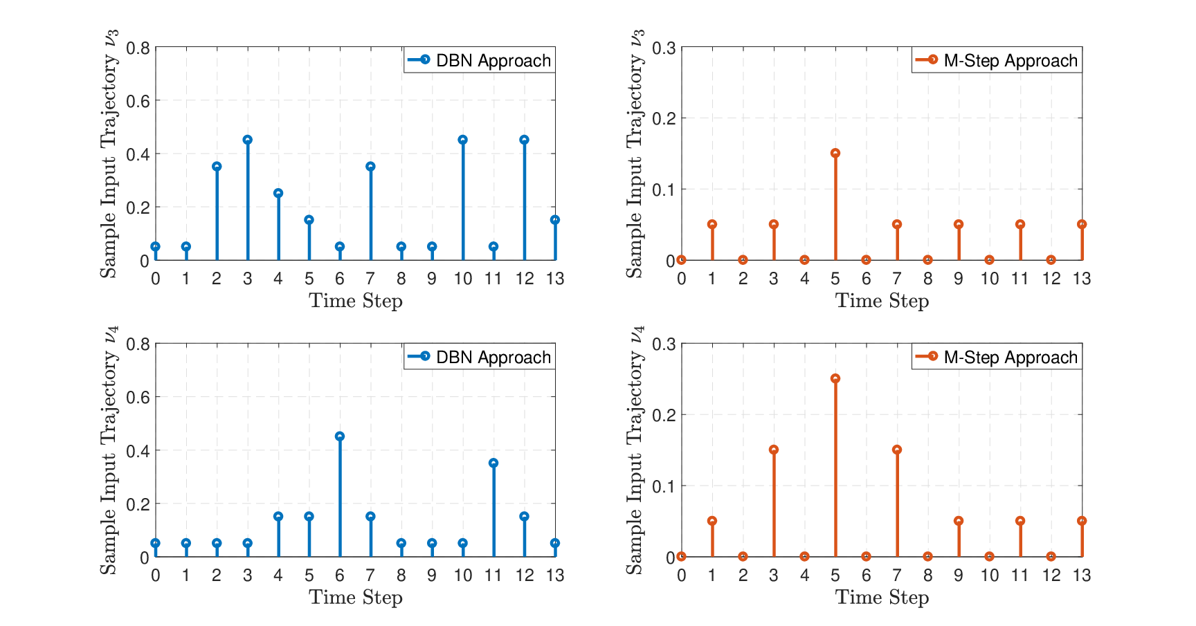
A comparison of safety probabilities for the $M$ -step and original subsystems is provided in Figure 2. We selected the initial conditions $x_{1}(0)=-0.35,x_{2}(0)=-0.285,x_{3}(0)=-1.705,x_{4}(0)=-1.745$ . In each plot of Figure 2, we fixed three of these initial states and showed the probability as a function of the other state. We also fixed the standard deviation of the noise as $\sigma_{i}=0.1,\forall i\in\{1,2\},\sigma_{i}=0.6,\forall i\in\{3,4\}$ . As seen, the safety probabilities using the DBN approach are better than those using $M$ -step approach. This is mainly due the fact that the external inputs in the $M$ -step setting are allowed to take non-zero values only at particular time instances (here at $2j+1,\,\,j=\{0,\dots,6\}$ ), which makes the controller synthesis problem more conservative (as discussed in Remark 2.5).

We now plot one realization of the input trajectories for the third and fourth subsystems in both $M$ -step and DBN approaches in Figure 3. As seen, the DBN approach allows taking nonzero input values at all time steps whereas the $M$ -step one only allows non-zero input values at $2j+1,\,\,j=\{0,\dots,6\}$ .

6.4. Road Traffic Network

In this subsection, we apply our results to a road traffic network in a circular cascade ring composed of $50$ cells, each of which has the length of $500$ meters with $1$ entry and $1$ way out, as depicted schematically in Figure 4, left. The model of this case study is borrowed from [LCGG13] by including stochasticity in the model as an additive noise.

The entry of each cell is controlled by a traffic light, denoted by $\nu_{i}=[0,1],\forall i\in\{1,\dots,n\}$ , that enables (green light) or not (red light) the vehicles to pass. In this model the length of a cell is in kilometers ( $0.5~km$ ), and the flow speed of the vehicles is $100$ kilometers per hour ( $km/h$ ). Moreover, during the sampling time interval $\tau$ , it is assumed that $6$ vehicles pass the entry controlled by the traffic light, and one quarter of vehicles goes out on the exit of each cell (ratio denoted $q$ ). We want to observe the density of the traffic $x_{i}$ , given in vehicles per cell, for each cell $i$ of the road.

The model of the interconnected system $\Sigma$ is described by:

\displaystyle x(k+1)=Ax(k)+B\nu(k)+R\varsigma(k),

where $A$ is a matrix with diagonal elements $a_{ii}=1-\frac{\tau v_{i}}{l_{i}}-q,i\in\{1,\dots,n\}$ , off-diagonal elements $a_{i+1,i}=\frac{\tau v_{i}}{l_{i}},i\in\{1,\dots,n-1\}$ , $a_{1,n}=\frac{\tau v_{n}}{l_{n}}$ , and all other elements are identically zero. Moreover, $B$ and $R$ are diagonal matrices with elements $b_{ii}=6$ , and $r_{ii}=0.83,i\in\{1,\dots,n\}$ , respectively. Furthermore, $x(k)=[x_{1}(k);\ldots;x_{n}(k)]$ , $\nu(k)=[\nu_{1}(k);\ldots;\nu_{n}(k)]$ , and $\varsigma(k)=[\varsigma_{1}(k);\ldots;\varsigma_{n}(k)]$ .

Now, by introducing the individual cells $\Sigma_{i}$ described as

\displaystyle x_{i}(k+1)

\displaystyle=(1-\frac{\tau v_{i}}{l_{i}}-q)x_{i}(k)+\frac{\tau v_{i-1}}{l_{i-1}}\mathsf{w}_{i}(k)+6\nu_{i}(k)+0.83\varsigma_{i}(k),

where $\mathsf{w}_{i}(k)=x_{i-1}(k)$ (with $x_{0}=x_{n}$ ), one can readily verify that $\Sigma=\mathcal{I}(\Sigma_{1},\ldots,\Sigma_{n})$ where the coupling matrix $G$ is given by elements $G_{i+1,i}=1,i\in\{1,\dots,n-1\}$ , $G_{1,n}=1$ , and all other elements are identically zero. We fix here $n=50$ and $\tau=6.48$ seconds. Then, one can readily verify that condition (5.8) (applied to original subsystems $\Sigma_{i}$ , $\forall i\in\{1,\ldots,n\}$ ) is satisfied with $\tilde{M}_{i}=1$ , $K_{i}=0$ , $\hat{\kappa}_{i}=0.99$ , $\bar{X}^{11}_{i}=(\frac{\tau v_{i}}{l_{i}})^{2}(1+\pi_{i})$ , $\bar{X}^{12}_{i}=\bar{X}^{21}_{i}=(1-\frac{\tau v_{i}}{l_{i}}-q)\frac{\tau v_{i}}{l_{i}}$ , $\bar{X}^{22}_{i}=-1.9(\frac{\tau v_{i}}{l_{i}})^{2}(1+\pi_{i})$ , $\forall i\in\{1,\dots,n\}$ , where $\pi_{i}=1.47$ . Hence, function $V_{i}(x_{i},\hat{x}_{i})=(x_{i}-\hat{x}_{i})^{2}$ is a classic storage function from $\widehat{\Sigma}_{i}$ to $\Sigma_{i}$ satisfying condition (3.1) with $\alpha_{i}(s)=s^{2}$ and condition (3.2) with $\kappa_{i}(s):=(1-\hat{\kappa}_{i})s$ , $\rho_{\mathrm{ext}i}(s)=0$ , $\forall s\in{\mathbb{R}}_{\geq 0}$ , $\psi_{i}=2.35\delta_{i}^{2}$ , and

\displaystyle\bar{X}_{i}=\begin{bmatrix}(\frac{\tau v_{i}}{l_{i}})^{2}(1+\pi_{i})~&~(1-\frac{\tau v_{i}}{l_{i}}-q)\frac{\tau v_{i}}{l_{i}}\\ (1-\frac{\tau v_{i}}{l_{i}}-q)\frac{\tau v_{i}}{l_{i}}~&~-1.9(\frac{\tau v_{i}}{l_{i}})^{2}(1+\pi_{i})\end{bmatrix}\!,~~i\in\{1,\dots,n\}.

(6.10)

Now, we look at $\widehat{\Sigma}=\widehat{\mathcal{I}}(\widehat{\Sigma}_{1},\ldots,\widehat{\Sigma}_{N})$ with a coupling matrix $\hat{G}$ satisfying condition (4.7) as $\hat{G}=G$ . Choosing $\mu_{1}=\cdots=\mu_{N}=1$ and using $\bar{X}_{i}$ in (6.10), condition (4.8) is satisfied as

	$\displaystyle\begin{bmatrix}G\\ \mathds{I}_{n}\end{bmatrix}^{T}\!\bar{X}_{cmp}\begin{bmatrix}G\\ \mathds{I}_{n}\end{bmatrix}=$	$\displaystyle(\frac{\tau v_{i}}{l_{i}})^{2}(1+\pi_{i})G^{T}G+(1-\frac{\tau v_{i}}{l_{i}}-q)\frac{\tau v_{i}}{l_{i}}(G^{T}+G)-1.9(\frac{\tau v_{i}}{l_{i}})^{2}(1+\pi_{i})\mathds{I}_{n}$
	$\displaystyle=$	$\displaystyle(1-\frac{\tau v_{i}}{l_{i}}-q)\frac{\tau v_{i}}{l_{i}}(G^{T}+G)-0.9(\frac{\tau v_{i}}{l_{i}})^{2}(1+\pi_{i})\mathds{I}_{n}\leq 0,$

without requiring any restrictions on the number or gains of the subsystems. Note that $G^{T}G$ is an identity matrix, and $G^{T}+G$ is a matrix with elements $\bar{g}_{i,i+1}=\bar{g}_{i+1,i}=\bar{g}_{1,n}=\bar{g}_{n,1}=1$ , $i\in\{1,\ldots,n-1\}$ , and all other elements are identically zero. In order to show the above inequality, we used, $i\in\{1,\dots,n\}$ ,

\displaystyle 2(1-\frac{\tau v_{i}}{l_{i}}-q)\frac{\tau v_{i}}{l_{i}}-0.9(\frac{\tau v_{i}}{l_{i}})^{2}(1+\pi_{i})\preceq 0,

employing Gershgorin circle theorem [Bel65]. Now, one can readily verify that $V(x,\hat{x})=\sum_{i=1}^{50}(x_{i}-\hat{x}_{i})^{2}$ is a classic simulation function from $\widehat{\Sigma}$ to $\Sigma$ satisfying conditions (8.8) and (8.9) with $\alpha(s)=s^{2}$ , $\kappa(s):=(1-\hat{\kappa})s$ , $\rho_{\mathrm{ext}}(s)=0$ , $\forall s\in{\mathbb{R}}_{\geq 0}$ , and $\psi=117.78\delta^{2}$ .

By taking the state set discretization parameter $\delta_{i}=0.02$ , and taking the initial states of the interconnected systems $\Sigma$ and $\widehat{\Sigma}$ as $10\mathds{1}_{50}$ , we guarantee that the distance between states of $\Sigma$ and of $\widehat{\Sigma}$ will not exceed $\varepsilon=1$ during the time horizon $T_{d}=10$ with probability at least $90\%$ , i.e.,

\displaystyle\mathbb{P}(\|x_{a\nu}(k)-\hat{x}_{\hat{a}\hat{\nu}}(k)\|\leq 1,\,\,\forall k\in[0,10])\geq 0.9.

(6.11)

Let us now synthesize a safety controller for $\Sigma$ via the abstraction $\widehat{\Sigma}$ such that the controller maintains the density of the traffic lower than $20$ vehicles per cell. The idea here is to first design a local controller for the abstraction $\widehat{\Sigma}_{i}$ , and then refine it back to the system $\Sigma_{i}$ using an interface function.

We employ here the software tool FAUST² [SGA15] by doing some slight modification to accept internal inputs as disturbances, and synthesize a controller for $\Sigma$ by taking the standard deviation of the noise to be $\sigma_{i}=0.83$ , $\forall i\in\{1,\ldots,n\}$ . The optimal policy for a representative cell in a network of $50$ cells is plotted in Figure 5, left. The obtained policy here is sub-optimal for each subsystem and is obtained by assuming that other subsystems do not violate their safety specifications. Closed-loop state trajectories of the representative cell with different noise realizations are illustrated in Figure 5 right, with only $10$ trajectories.

For the construction of finite abstractions, we have selected the center of partition sets as representative points. Moreover, we assume a well-defined interconnection of abstractions (i.e. $\hat{G}\prod_{i=1}^{N}\hat{X}=\prod_{i=1}^{N}\hat{W}_{i}$ ). Then satisfying compositionality condition (4.6) is no more needed, and accordingly, the overall error formulated in (8.1) is reduced to $\psi=\sum_{i=1}^{N}\mu_{i}\psi_{i}$ .

Note that since the property of interest in this example is invariance, we employed FAUST to perform synthesis in a fully decentralized manner by considering states of other subsystems inside bounded internal input sets. The synthesis framework then is reduced to a $\max$ - $\min$ optimization problem (using the standard dynamic programming) for two and a half player games by considering the internal and external inputs of the system as the corresponding players [KDS+11]. In particular, we consider the internal input affecting the system as an adversary and maximize the probability of satisfaction under the worst-case strategy of a rational adversary. Therefore, one should minimize the probability of satisfaction with respect to internal inputs and then maximize it with respect to external ones.

In order to perform the compositional controller synthesis, we leverage the assume-guarantee reasoning [HQR98] by assuming that while we perform the synthesis for a subsystem, other subsystems do not violate their invariant specifications (i.e., their states stay inside internal input sets). Roughly speaking, an assume-guarantee contract for a discrete-time system intuitively states that if the internal input of the system belongs to a set (described by a set of assumptions) within a time horizon $l\in\mathbb{N}$ , then the state of the system belongs to a set (described by a set of guarantees) within the same time horizon $l$ [SGF18]. The recent work [SGF18] in the non-stochastic setting allows one to reason about interconnected systems based on contracts satisfied by subsystems under additional requirements. In the stochastic setting, we obtain local controllers that are sub-optimal for the safety probability of the whole network.

6.5. Nonlinear Fully Interconnected Network

In order to show applicability of our approach to strongly connected networks with nonlinear dynamics (cf. Figure 4, right), we consider nonlinear SCS

\Sigma:x(k+1)=\bar{G}x(k)+\varphi(x(k))+\nu(k)+\varsigma(k),

for some matrix $\bar{G}=(\mathds{I}_{n}-\bar{\tau}L)\in\mathbb{R}^{n\times n}$ where $\bar{\tau}L$ is the Laplacian matrix of an undirected graph with $0<\bar{\tau}<1/\Delta$ , and $\Delta$ is the maximum degree of the graph [GR01]. We assume $L$ is the Laplacian matrix of a complete graph as

\displaystyle L=\begin{bmatrix}n-1&-1&\cdots&\cdots&-1\\ -1&n-1&-1&\cdots&-1\\ -1&-1&n-1&\cdots&-1\\ \vdots&&\ddots&\ddots&\vdots\\ -1&\cdots&\cdots&-1&n-1\end{bmatrix}_{n\times n}\!\!\!\!\!\!\!\!\!\!\!\!.

(6.12)

Moreover, $\varsigma(k)=[\varsigma_{1}(k);\ldots;\varsigma_{N}(k)]$ , $\varphi(x(k))=[E_{1}\varphi_{1}(F_{1}x_{1}(k));\ldots;E_{N}\varphi_{N}(F_{N}x_{N}(k))]$ where $\varphi_{i}(x)=sin(x)$ , $\forall i\in\{1,\ldots,N\}$ . We partition $x(k)$ as $x(k)=[x_{1}(k);\ldots;x_{N}(k)]$ and $\nu(k)$ as $\nu(k)=[\nu_{1}(k);\ldots;\nu_{N}(k)]$ . Now, by introducing $\Sigma_{i}$ described as

\Sigma_{i}:x_{i}(k+1)=x_{i}(k)+E_{i}\varphi_{i}(F_{i}x_{i}(k))+\nu_{i}(k)+\mathsf{w}_{i}(k)+\varsigma_{i}(k),

one can verify that $\Sigma=\mathcal{I}(\Sigma_{1},\ldots,\Sigma_{N})$ where the coupling matrix $G$ is given by $G=-\bar{\tau}L$ . Then, one can readily verify that, $\forall i\in\{1,\ldots,N\}$ , condition (5.7) is satisfied with $\tilde{M}_{i}=1$ , $K_{i}=-0.5$ , $E_{i}=0.1$ , $F_{i}=0.1$ , $\tilde{b}_{i}=1$ , $\bar{X}^{11}=(1+\pi_{i})$ , $\bar{X}^{22}=0$ , $\bar{X}^{12}=\bar{X}^{21}=\lambda_{i}$ , where $\lambda_{i}=1+K_{i}$ , $\hat{\kappa}_{i}=0.99$ , and $\pi_{i}=1$ , $\forall i\in\{1,\ldots,N\}$ . Hence, function $V_{i}(x_{i},\hat{x}_{i})=(x_{i}-\hat{x}_{i})^{2}$ is a classic storage function from $\widehat{\Sigma}_{i}$ to $\Sigma_{i}$ satisfying condition (3.1) with $\alpha_{i}(s)=s^{2}$ and condition (3.2) with $\kappa_{i}(s):=(1-\hat{\kappa}_{i})s$ , $\rho_{\mathrm{iext}}(s)=0$ , $\forall s\in{\mathbb{R}}_{\geq 0}$ , and $\psi_{i}=4\delta_{i}^{2}$ . Now, we look at $\widehat{\Sigma}=\widehat{\mathcal{I}}(\widehat{\Sigma}_{1},\ldots,\widehat{\Sigma}_{N})$ with a coupling matrix $\hat{G}$ satisfying condition (4.7) by $\hat{G}=G$ . Choosing $\mu_{1}=\cdots=\mu_{N}=1$ , matrix $\bar{X}_{cmp}$ in (4.9) reduces to

\bar{X}_{cmp}=\begin{bmatrix}(1+\pi)\mathds{I}_{n}&\lambda\mathds{I}_{n}\\ \lambda\mathds{I}_{n}&0\end{bmatrix}\!,

where $\lambda=\lambda_{1}=\cdots=\lambda_{n}$ , $\pi=\pi_{1}=\cdots=\pi_{n}$ , and condition (4.8) reduces to

\displaystyle\begin{bmatrix}-\bar{\tau}L\\ \mathds{I}_{n}\end{bmatrix}^{T}\!\bar{X}_{cmp}\begin{bmatrix}-\bar{\tau}L\\ \mathds{I}_{n}\end{bmatrix}=(1+\pi)\bar{\tau}^{2}L^{T}L-\lambda\bar{\tau}L-\lambda\bar{\tau}L^{T}=\bar{\tau}L((1+\pi)\bar{\tau}L-2\lambda\mathds{I}_{n})\preceq 0,

which is always satisfied without requiring any restrictions on the number or gains of the subsystems with $\bar{\tau}=0.4/(n-1)$ . In order to show the above inequality, we used $\bar{\tau}L=\bar{\tau}L^{T}\succeq 0$ which is always true for Laplacian matrices of undirected graphs. We fix here $n=500$ . Now, one can verify that $V(x,\hat{x})=\sum_{i=1}^{500}(x_{i}-\hat{x}_{i})^{2}$ is a classic simulation function from $\widehat{\Sigma}$ to $\Sigma$ satisfying conditions (8.8) and (8.9) with $\alpha(s)=s^{2}$ , $\kappa(s):=(1-\hat{\kappa})s$ , $\rho_{\mathrm{ext}}(s)=0$ , $\forall s\in{\mathbb{R}}_{\geq 0}$ , and $\psi=2000\delta^{2}$ .

By taking the state discretization parameter $\delta=0.005$ , using the stochastic simulation function $V$ , inequality (3.4), and selecting the initial states of the interconnected systems $\Sigma$ and $\widehat{\Sigma}$ as $\mathds{1}_{500}$ , we guarantee that the distance between states of $\Sigma$ and of $\widehat{\Sigma}$ will not exceed $\varepsilon=1$ during the time horizon $T_{d}=10$ with the probability at least $88\%$ .

7. Discussion

In this paper, we provided a compositional approach for the construction of finite MDPs for networks of not necessarily stabilizable stochastic systems. We first introduced new notions of finite-step stochastic storage and simulation functions to quantify the probabilistic mismatch between the systems. We then developed a compositional framework on the construction of finite MDPs for networks of stochastic systems using a new type of dissipativity-type conditions. By employing this relaxation via finite-step stochastic simulation function, it is possible to construct finite abstractions such that the stabilizability of each subsystem is not necessarily required. Afterwards, we proposed an approach to construct finite MDPs together with their corresponding finite-step stochastic storage functions for general stochastic control systems satisfying some incremental passivablity property. We showed that for two classes of nonlinear and linear stochastic control systems, the aforementioned property can be readily checked by some matrix inequalities. We then constructed finite MDPs with their classic storage functions for a particular class of nonlinear stochastic control systems. Finally, we demonstrated the effectiveness of our proposed approaches by applying our results to three different case studies.

References

[AMP16] M. Arcak, C. Meissen, and A. Packard. Networks of dissipative systems. SpringerBriefs in Electrical and Computer Engineering. Springer, 2016.
[Ang02] D. Angeli. A Lyapunov approach to incremental stability properties. IEEE Transactions on Automatic Control, 47(3):410–421, March 2002.
[AP98] D. Aeyels and J. Peuteman. A new asymptotic stability criterion for nonlinear time-variant differential equations. IEEE Transactions on automatic control, 43(7):968–971, 1998.
[APLS08] A. Abate, M. Prandini, J. Lygeros, and S. Sastry. Probabilistic reachability and safety for controlled discrete time stochastic hybrid systems. Automatica, 44(11):2724–2734, 2008.
[Bel65] H. E. Bell. Gershgorin’s theorem and the zeros of polynomials. The American Mathematical Monthly, 72(3):292–295, 1965.
[BK08] C. Baier and J.P. Katoen. Principles of model checking. MIT press, 2008.
[BKW14] N. Basset, M. Kwiatkowska, and C. Wiltsche. Compositional controller synthesis for stochastic games. In Proceedings of the International Conference on Concurrency Theory, pages 173–187, 2014.
[BS96] D. P. Bertsekas and S. E. Shreve. Stochastic Optimal Control: The Discrete-Time Case. Athena Scientific, 1996.
[DAK12] A. D’Innocenzo, A. Abate, and J.P. Katoen. Robust PCTL model checking. In Proceedings of the 15th ACM International Conference on Hybrid Systems: Computation and Control, pages 275–286, 2012.
[DLT08] J. Desharnais, F. Laviolette, and M. Tracol. Approximate analysis of probabilistic processes: Logic, simulation and games. In Proceedings of the 5th International Conference on Quantitative Evaluation of System, pages 264–273, 2008.
[GGLW14] R. Geiselhart, R. H. Gielen, M. Lazar, and F. R. Wirth. An alternative converse Lyapunov theorem for discrete-time systems. Systems & Control Letters, 70:49–59, 2014.
[GL12] R. H. Gielen and M. Lazar. Non-conservative dissipativity and small-gain conditions for stability analysis of interconnected systems. In Proceedings of the 51st IEEE Conference on Decision and Control (CDC), pages 4187–4192, 2012.
[GL15] R. H. Gielen and M. Lazar. On stability analysis methods for large-scale discrete-time systems. Automatica, 55:66–72, 2015.
[GR01] C. Godsil and G. Royle. Algebraic graph theory. Graduate Texts in Mathematics. Springe, New York, 2001.
[HHHK13] E. M. Hahn, A. Hartmanns, H. Hermanns, and J.-P. Katoen. A compositional modelling and analysis framework for stochastic hybrid systems. Formal Methods in System Design, 43(2):191–232, 2013.
[HQR98] T. A. Henzinger, S. Qadeer, and S. K. Rajamani. You assume, we guarantee: Methodology and case studies. In International Conference on Computer Aided Verification, pages 440–451, 1998.
[HS18] Sofie Haesaert and Sadegh Soudjani. Robust dynamic programming for temporal logic control of stochastic systems. CoRR, abs/1811.11445, 2018.
[HSA17] S. Haesaert, S. Soudjani, and A. Abate. Verification of general Markov decision processes by approximate similarity relations and policy refinement. SIAM Journal on Control and Optimization, 55(4):2333–2367, 2017.
[JP09] A. A. Julius and G. J. Pappas. Approximations of stochastic hybrid systems. IEEE Transactions on Automatic Control, 54(6):1193–1203, 2009.
[KDS⁺11] M. Kamgarpour, J. Ding, S. Summers, A. Abate, J. Lygeros, and C. Tomlin. Discrete time stochastic hybrid dynamical games: Verification & controller synthesis. In Proceedings of the 50th IEEE Conference on Decision and Control and European Control Conference, pages 6122–6127, 2011.
[KNPQ13] M. Kwiatkowska, G. Norman, D. Parker, and H. Qu. Compositional probabilistic verification through multi-objective model checking. Information and Computation, 232:38–65, 2013.
[LCGG13] E.l Le Corronc, A. Girard, and G. Goessler. Mode sequences as symbolic states in abstractions of incrementally stable switched systems. In Proceedings of the 52th IEEE Conference on Decision and Control, pages 3225–3230, 2013.
[LS91] K. G. Larsen and A. Skou. Bisimulation through probabilistic testing. Information and Computation, 94(1):1–28, 1991.
[LSMZ17] A. Lavaei, S. Soudjani, R. Majumdar, and M. Zamani. Compositional abstractions of interconnected discrete-time stochastic control systems. In Proceedings of the 56th IEEE Conference on Decision and Control, pages 3551–3556, 2017.
[LSZ18a] A. Lavaei, S. Soudjani, and M. Zamani. Compositional synthesis of finite abstractions for continuous-space stochastic control systems: A small-gain approach. In Proceedings of the 6th IFAC Conference on Analysis and Design of Hybrid Systems, volume 51, pages 265–270, 2018.
[LSZ18b] A. Lavaei, S. Soudjani, and M. Zamani. From dissipativity theory to compositional construction of finite Markov decision processes. In Proceedings of the 21st ACM International Conference on Hybrid Systems: Computation and Control, pages 21–30, 2018.
[LSZ19a] A. Lavaei, S. Soudjani, and M. Zamani. Approximate probabilistic relations for compositional synthesis of stochastic systems. In Proceedings of the Numerical Software Verification, pages 101–109, 2019. Lecture Notes in Computer Science 11652.
[LSZ19b] A. Lavaei, S. Soudjani, and M. Zamani. Compositional abstraction-based synthesis of general MDPs via approximate probabilistic relations. arXiv:1906.02930, 2019.
[LSZ19c] A. Lavaei, S. Soudjani, and M. Zamani. Compositional construction of infinite abstractions for networks of stochastic control systems. Automatica, 107:125–137, 2019.
[LSZ19d] A. Lavaei, S. Soudjani, and M. Zamani. Compositional synthesis of not necessarily stabilizable stochastic systems via finite abstractions. In Proceedings of the 18th European Control Conference, pages 2802–2807, 2019.
[LSZ20a] A. Lavaei, S. Soudjani, and M. Zamani. Compositional abstraction-based synthesis for networks of stochastic switched systems. Automatica, 114, 2020.
[LSZ20b] A. Lavaei, S. Soudjani, and M. Zamani. Compositional (in)finite abstractions for large-scale interconnected stochastic systems. IEEE Transactions on Automatic Control, to appear as a full paper, arXiv: 1808.00893, 2020.
[LZ19] A. Lavaei and M. Zamani. Compositional construction of finite MDPs for large-scale stochastic switched systems: A dissipativity approach. Proceedings of the 15th IFAC Symposium on Large Scale Complex Systems: Theory and Applications, 52(3):31–36, 2019.
[LZ20] A. Lavaei and M. Zamani. Compositional verification of large-scale stochastic systems via relaxed small-gain conditions. In Proceedings of the 58th IEEE Conference on Decision and Control, 2020.
[NGG⁺18] N. Noroozi, R. Geiselhart, L. Grüne, B. S. Rüffer, and F. R. Wirth. Nonconservative discrete-time ISS small-gain conditions for closed sets. IEEE Transactions on Automatic Control, 63(5):1231–1242, 2018.
[NR14] Navid Noroozi and Björn S Rüffer. Non-conservative dissipativity and small-gain theory for ISS networks. In Proceedings of the 53rd IEEE Conference on Decision and Control, pages 3131–3136, 2014.
[NSWZ18] N. Noroozi, A. Swikir, F. R. Wirth, and M. Zamani. Compositional construction of abstractions via relaxed small-gain conditions part ii: discrete case. In 2018 European Control Conference (ECC), pages 1–4, 2018.
[NSZ19] A. Nejati, S. Soudjani, and M. Zamani. Abstraction-based synthesis of continuous-time stochastic control systems. In Proceedings of the 18th European Control Conference, pages 3212–3217, 2019.
[PTS09] Q. C. Pham, N. Tabareau, and J. J. Slotine. A contraction theory approach to stochastic incremental stability. IEEE Transactions on Automatic Control, 54(4):816–820, 2009.
[SA13] S. Soudjani and A. Abate. Adaptive and sequential gridding procedures for the abstraction and verification of stochastic processes. SIAM Journal on Applied Dynamical Systems, 12(2):921–956, 2013.
[SA15] Sadegh Soudjani and Alessandro Abate. Quantitative approximation of the probability distribution of a Markov process by formal abstractions. Logical Methods in Computer Science, 11(3), 2015.
[SAM17] Sadegh Soudjani, Alessandro Abate, and Rupak Majumdar. Dynamic Bayesian networks for formal verification of structured stochastic processes. Acta Informatica, 54(2):217–242, Mar 2017.
[SGA15] S. Soudjani, C. Gevaerts, and A. Abate. FAUST ${}^{\textsf{2}}$ : Formal abstractions of uncountable-state stochastic processes. In TACAS’15, volume 9035 of Lecture Notes in Computer Science, pages 272–286. Springer, 2015.
[SGF18] A. Saoud, A. Girard, and L. Fribourg. On the composition of discrete and continuous-time assume-guarantee contracts for invariance. In 2018 European Control Conference (ECC), pages 435–440, 2018.
[SL95] R. Segala and N. Lynch. Probabilistic simulations for probabilistic processes. Nordic Journal of Computing, 2(2):250–273, 1995.
[TA11] I. Tkachev and A. Abate. On infinite-horizon probabilistic properties and stochastic bisimulation functions. In Proceedings of the 50th IEEE Conference on Decision and Control and European Control Conference (CDC-ECC), pages 526–531, 2011.
[TMKA13] I. Tkachev, A. Mereacre, J.-P. Katoen, and A. Abate. Quantitative automata-based controller synthesis for non-autonomous stochastic hybrid systems. In Proceedings of the 16th ACM International Conference on Hybrid Systems: Computation and Control, pages 293–302, 2013.
[You12] W. H. Young. On classes of summable functions and their fourier series. Proceedings of the Royal Society of London A: Mathematical, Physical and Engineering Sciences, 87(594):225–229, 1912.
[ZA14] M. Zamani and A. Abate. Approximately bisimilar symbolic models for randomly switched stochastic systems. Systems & Control Letters, 69:38–46, 2014.
[ZAG15] M. Zamani, A. Abate, and A. Girard. Symbolic models for stochastic switched systems: A discretization and a discretization-free approach. Automatica, 55:183–196, 2015.
[ZMEM⁺14] M. Zamani, P. Mohajerin Esfahani, R. Majumdar, A. Abate, and J. Lygeros. Symbolic control of stochastic systems via approximately bisimilar finite abstractions. IEEE Transactions on Automatic Control, 59(12):3135–3150, 2014.
[ZRME17] M. Zamani, M. Rungger, and P. Mohajerin Esfahani. Approximations of stochastic hybrid systems: A compositional approach. IEEE Transactions on Automatic Control, 62(6):2838–2853, 2017.

8. Appendix

8.1. Technical Discussions

$M$ -Sampled Systems.

Example 8.1.

(for Lemma 2.6) Consider linear SCS $\Sigma_{i}$ , $i\in\{1,2\}$ , with dynamics

\displaystyle\Sigma_{i}:x_{i}(k+1)=A_{i}x_{i}(k)+B_{i}\nu_{i}(k)+D_{i}\mathsf{w}_{i}(k)+R_{i}\varsigma_{i}(k),

(8.1)

connected with constraints $[{\mathsf{w}_{1};\mathsf{w}_{2}}]=\begin{bmatrix}G_{11}&G_{12}\\ G_{21}&G_{22}\\ \end{bmatrix}[{x_{1};x_{2}}]$ . Matrices $A_{i},B_{i},D_{i},R_{i}$ , $i\in\{1,2\}$ , have appropriate dimensions. We can rewrite the given dynamics as

\displaystyle{x}(k+1)=\bar{A}x(k)+\bar{B}\nu(k)+\bar{D}\mathsf{w}(k)+\bar{R}\varsigma(k),

with $x=[{x_{1};x_{2}}],\nu=[{\nu_{1};\nu_{2}}],\mathsf{w}=[{\mathsf{w}_{1};\mathsf{w}_{2}}],\varsigma=[{\varsigma_{1};\varsigma_{2}}]$ , where

\displaystyle\bar{A}=\mathsf{diag}(A_{1},A_{2}),\bar{B}=\mathsf{diag}(B_{1},B_{2}),\bar{D}=\mathsf{diag}(D_{1},D_{2}),\bar{R}=\mathsf{diag}(R_{1},R_{2}).

By applying the interconnection constraints $\mathsf{w}=[{\mathsf{w}_{1};\mathsf{w}_{2}}]=G[{x_{1};x_{2}}]$ with $G=\begin{bmatrix}G_{11}&G_{12}\\ G_{21}&G_{22}\\ \end{bmatrix}$ , we have

x(k+1)=(\bar{A}+\bar{D}G)x(k)+\bar{B}\nu(k)+\bar{R}\varsigma(k).

Now by looking at the solutions $M$ steps ahead, one gets

\displaystyle x(k+M)=

\displaystyle(\bar{A}+\bar{D}G)^{M}x(k)+\sum_{n=0}^{M-1}(\bar{A}+\bar{D}G)^{n}\bar{B}\nu(k+M-n-1)+\sum_{n=0}^{M-1}(\bar{A}+\bar{D}G)^{n}\bar{R}\varsigma(k+M-n-1).

After applying Assumption 1 and by partitioning $(\bar{A}+\bar{D}G)^{M}$ as

\displaystyle(\bar{A}+\bar{D}G)^{M}=\left[\begin{array}[]{c|c}\tilde{A}_{1}&\tilde{D}_{1}\\ \hline\cr\tilde{A}_{2}&\tilde{D}_{2}\end{array}\right]\!,

one can decompose the network and obtain the auxiliary subsystems proposed in (2.8) as follows, $i\in\{1,2\}$ :

\displaystyle\Sigma_{\textsf{aux}i}:x_{i}(k+M)

\displaystyle=\tilde{A}_{i}x_{i}(k)+B_{i}\nu_{i}(k+M-1)+\tilde{D}_{i}w_{i}(k)+\tilde{R}_{i}\tilde{\varsigma}_{i}(k),

(8.4)

where $w_{1}(k),w_{2}(k)$ are the new internal inputs, $\tilde{\varsigma}_{1}(k),\tilde{\varsigma}_{2}(k)$ are defined as in (2.9) with $N=2$ , and $\tilde{R}_{i}$ is a matrix of appropriate dimension which can be computed based on the matrices in (8.1). As seen, $\tilde{A}_{1}$ and $\tilde{A}_{2}$ now depend also on $D_{1},D_{2}$ and the interconnection matrix $G$ , which may result in the pairs $(\tilde{A}_{1},B_{1})$ and $(\tilde{A}_{2},B_{2})$ being stabilizable.

Remark 8.2.

The main idea behind the proposed approach is that we first look at the solutions of the unstabilizable subsystems, during which we interconnect the subsystems with each other based on their interconnection networks. We go ahead until all subsystems are stabilizable (if possible). Once the stabilizing effect is evident, we decompose the network such that each subsystem is only in terms of its own state, and external input. In contrast to the given original systems, the interconnection topology will change, meaning that the internal input of the auxiliary system is different from the original one. Moreover, the external input of the auxiliary system after doing the $M$ -step analysis is given only at instants $k+M-1$ , $k=jM$ , $j\in\mathbb{N}$ . Finally, the noise term in the auxiliary system is now a sequence of noises of other subsystems in different time steps depending on the type of interconnection.

Construction of Finite MDPs. Dynamical representation provided by Theorem 2.7 uses the map $\Pi_{x}:X\rightarrow\hat{X}$ that satisfies the inequality

\|\Pi_{x}(x)-x\|\leq\delta,\quad\forall x\in X,

(8.5)

where $\delta:=\sup\{\|x-x^{\prime}\|,\,\,x,x^{\prime}\in\mathsf{X}_{i},\,i=1,2,\ldots,n_{x}\}$ is the state discretization parameter. Let us similarly define the abstraction map $\Pi_{w}:\tilde{W}\rightarrow\hat{W}$ on $\tilde{W}$ that assigns to any $w\in W$ a representative point $\hat{w}\in\hat{W}$ of the corresponding partition set containing $w$ . This map also satisfies

\|\Pi_{w}(w)-w\|\leq\beta,\,\quad\forall w\in\tilde{W},

(8.6)

where $\beta$ is the internal input discretization parameter defined similar to $\delta$ . We used inequality (8.6) in Section 4 for the compositional construction of abstractions for interconnected systems.

Remark 8.3.

Note that condition (8.6) helps us to choose quantization parameters of internal input sets freely at the cost of incurring an additional error term for the overall network (i.e, $\psi$ ) which is formulated based on $\beta$ in (8.1). Moreover, the state discretization parameter $\delta$ appears in the formulated error for each subsystem (i.e, $\psi_{i}$ ) as in (8.17) and (8.18). These two errors together affect the probabilistic closeness guarantee provided in Theorem 3.2.

Algorithm 1 Abstraction of SCS

\Sigma_{\textsf{aux}}

by a finite MDP

\widehat{\Sigma}_{\textsf{aux}}

0: input SCS

\Sigma_{\textsf{aux}}

1: Select finite partitions of sets

X,U,\tilde{W}

X=\cup_{i=1}^{n_{x}}\mathsf{X}_{i}

U=\cup_{i=1}^{n_{\nu}}\mathsf{U}_{i}

\tilde{W}=\cup_{i=1}^{n_{w}}\mathsf{\tilde{W}_{i}}

2: For each

\mathsf{X}_{i},\mathsf{U}_{i}

, and

\mathsf{\tilde{W}_{i}}

, select single representative points

\hat{x}_{i}\in\mathsf{X}_{i}

\hat{\nu}_{i}\in\mathsf{U}_{i}

\hat{w}_{i}\in\mathsf{\tilde{W}_{i}}

3: Define

\hat{X}:=\{\hat{x}_{i},i=1,...,n_{x}\}

as the finite state set of MDP

\widehat{\Sigma}_{\textsf{aux}}

with external and internal input sets

\hat{U}:=\{\hat{\nu}_{i},i=1,...,n_{\nu}\}

\hat{W}:=\{\hat{w}_{i},i=1,...,n_{w}\}

4: Define the map

\Xi:X\rightarrow 2^{X}

that assigns to any

x\in X

, the corresponding partition set it belongs to, i.e.,

\Xi(x)=\mathsf{X}_{i}

x\in\mathsf{X}_{i}

for some

i=1,2,\ldots,n_{x}

5: Compute the discrete transition probability matrix

\hat{T}_{\mathsf{x}}

for

\widehat{\Sigma}_{\textsf{aux}}

as:

\displaystyle\hat{T}_{\mathsf{x}}(x^{\prime}|x,\nu,w)=T_{\mathsf{x}}(\Xi(x^{\prime})|x,\nu,w),

(8.7)

for all

x:=x(k),x^{\prime}:=x(k+M)\in\hat{X},\nu:=\nu(k+M-1)\in\hat{U},w:=w(k)\in\hat{W}

k=jM,j\in{\mathbb{N}}

5: output finite MDP

\widehat{\Sigma}_{\textsf{aux}}

Finite-Step Simulation Functions.

Definition 8.4.

Consider two SCS $\Sigma$ and $\widehat{\Sigma}$ without internal inputs, where $\hat{X}\subseteq X$ . A function $V:X\times\hat{X}\to{\mathbb{R}}_{\geq 0}$ is called a finite-step stochastic simulation function (FSF) from $\widehat{\Sigma}$ to $\Sigma$ if there exist $M\in\mathbb{N}_{\geq 1}$ , and $\alpha\in\mathcal{K}_{\infty}$ such that

\displaystyle\forall x:=x(k)\in X,\forall\hat{x}:=\hat{x}(k)\in\hat{X},\quad\alpha(\|x-\hat{x}\|)\leq V(x,\hat{x}),

(8.8)

and $\forall x:=x(k)\in X,\,\forall\hat{x}:=\hat{x}(k)\in\hat{X},\,\forall\hat{\nu}:=\hat{\nu}(k+M-1)\in\hat{U}$ , $\exists\nu:=\nu(k+M-1)\in U$ such that

\displaystyle\mathbb{E}

\displaystyle\Big[V(x(k+M),\hat{x}(k+M))\,\big|\,x,\hat{x},\nu,\hat{\nu}\Big]-V(x,\hat{x})\leq-\kappa(V(x,\hat{x}))+\rho_{\mathrm{ext}}(\|\hat{\nu}\|)+\psi,

(8.9)

for some $\kappa\in\mathcal{K}$ , $\rho_{\mathrm{ext}}\in\mathcal{K}_{\infty}\cup\{0\}$ , $\psi\in\mathbb{R}_{\geq 0}$ , and $k=jM,j\in{\mathbb{N}}$ .

If there exists an FSF $V$ from $\widehat{\Sigma}$ to $\Sigma$ , denoted by $\widehat{\Sigma}\preceq\Sigma$ , $\widehat{\Sigma}$ is called an abstraction of $\Sigma$ .

Analysis on Probabilistic Closeness Guarantees for Road Traffic Network. In order to have more practical analysis on the proposed probabilistic closeness guarantee, we plotted the probabilistic error bound provided in (3.4) in terms of the state discretization parameter $\delta$ and confidence bound $\varepsilon$ in Figure 6. As seen, the probabilistic closeness guarantee is improved by either decreasing $\delta$ or increasing $\varepsilon$ . Note that the constant $\psi$ in (3.4) is formulated based on the state discretization parameter $\delta$ as in (8.18). It is worth mentioning that there are some other parameters in (3.4) such as $\mathcal{K}_{\infty}$ function $\alpha$ , and the value of FSF $V$ at initial conditions $a,\hat{a}$ which can also improve our proposed closeness guarantee for different values of $T_{d}$ .

{IEEEproof}

(Theorem 2.7) It is sufficient to show that (8.7) holds for dynamical representation of $\widehat{\Sigma}_{\textsf{aux}}$ and that of $\Sigma_{\textsf{aux}}$ . For any $x:=x(k),x^{\prime}:=x^{\prime}(k+M)\in\hat{X}$ , $\nu:=\nu(k+M-1)\in\hat{U}$ and $w:=w(k)\in\hat{W}$ ,

\displaystyle\hat{T}_{\mathsf{x}}(x^{\prime}|x,\nu,w)

\displaystyle=\mathbb{P}(x^{\prime}=\hat{f}(x,\nu,w,\varsigma))=\mathbb{P}(x^{\prime}=\Pi_{x}(\tilde{f}(x,\nu,w,\varsigma)))=\mathbb{P}(\tilde{f}(x,\nu,w,\varsigma)\in\Xi(x^{\prime})),

where $\Xi(x^{\prime})$ is the partition set with $x^{\prime}$ as its representative point as defined in Step 4 of Algorithm 1. Using the probability measure $\vartheta(\cdot)$ of random variable $\varsigma$ , we can write

\displaystyle\hat{T}_{\mathsf{x}}(x^{\prime}|x,\nu,w)=\int_{\Xi(x^{\prime})}\tilde{f}(x,\nu,w,\varsigma)d\vartheta(\varsigma)=T_{\mathsf{x}}(\Xi(x^{\prime})|x,\nu,w),

which completes the proof.

{IEEEproof}

(Theorem 4.5) We first show that FSF $V$ in (4.5) satisfies the inequality (8.8) for some $\mathcal{K}_{\infty}$ function $\alpha$ . For any $x={\left[x_{1};\ldots;x_{N}\right]}\in X$ and $\hat{x}={\left[\hat{x}_{1};\ldots;\hat{x}_{N}\right]}\in\hat{X}$ , one gets:

\displaystyle\|

\displaystyle x-\hat{x}\|\leq\sum_{i=1}^{N}\|x_{i}-\hat{x}_{i}\|\leq\sum_{i=1}^{N}\alpha_{i}^{-1}(V_{i}(x_{i},\hat{x}_{i}))\leq\bar{\alpha}(V(x,\hat{x})),

with function $\bar{\alpha}:\mathbb{R}_{\geq 0}\rightarrow\mathbb{R}_{\geq 0}$ defined for all $r\in\mathbb{R}_{\geq 0}$ as

$\bar{\alpha}(r):=\max\left\{\sum_{i=1}^{N}\alpha_{i}^{-1}(s_{i})\,\,\big|\,s_{i}{\geq 0},\,\,\sum_{i=1}^{N}\mu_{i}s_{i}=r\right\}.$

It is not hard to verify that function $\bar{\alpha}(\cdot)$ defined above is a $\mathcal{K}_{\infty}$ function. By taking the $\mathcal{K}_{\infty}$ function $\alpha(r):=\bar{\alpha}^{-1}(r)$ , $\forall r\in{\mathbb{R}}_{\geq 0}$ , one obtains

\alpha(\|x-\hat{x}\|)\leq V(x,\hat{x}),

satisfying inequality (8.8). Now we prove that FSF $V$ in (4.5) satisfies inequality (8.9), as well. Consider any $x={\left[x_{1};\ldots;x_{N}\right]}\in X$ , $\hat{x}={\left[\hat{x}_{1};\ldots;\hat{x}_{N}\right]}\in\hat{X}$ , and $\hat{\nu}={\left[\hat{\nu}_{1};\ldots;\hat{\nu}_{N}\right]}\in\hat{U}$ . For any $i\in\{1,\ldots,N\}$ , there exists $\nu_{i}\in U_{i}$ , consequently, a vector $\nu={\left[\nu_{1};\ldots;\nu_{N}\right]}\in U$ , satisfying (3.2) for each pair of subsystems $\Sigma_{i}$ and $\widehat{\Sigma}_{i}$ with the internal inputs given by ${\left[w_{1};\ldots;w_{N}\right]}=G_{a}[x_{1};\ldots;x_{N}]$ and ${\left[\hat{w}_{1};\ldots;\hat{w}_{N}\right]}=\Pi_{w}(\hat{G}_{a}[\hat{x}_{1};\ldots;\hat{x}_{N}])$ . By defining ${\left[\bar{w}_{1};\ldots;\bar{w}_{N}\right]}=\hat{G}_{a}[\hat{x}_{1};\ldots;\hat{x}_{N}]$ , we obtain the chain of inequalities in (8.11) using conditions (4.6), (4.7), (4.8) and by defining $\kappa(\cdot),\rho_{\mathrm{ext}}(\cdot),\psi$ as

	$\displaystyle\kappa(r)$	$\displaystyle:=(1-\bar{\mu})\min\Big\{\sum_{i=1}^{N}\mu_{i}\kappa_{i}(s_{i})\,\,\big\|\,s_{i}{\geq 0},\sum_{i=1}^{N}\mu_{i}s_{i}=r\Big\}$
	$\displaystyle\rho_{\mathrm{ext}}(r)$	$\displaystyle:=\max\Big\{\sum_{i=1}^{N}\mu_{i}\rho_{\mathrm{ext}i}(s_{i})\,\big\|\,s_{i}{\geq 0},\\|{\left[s_{1};\ldots;s_{N}\right]}\\|=r\Big\},$
	$\displaystyle\psi$	$\displaystyle:=\begin{cases}\sum_{i=1}^{N}\mu_{i}\psi_{i}+\frac{\\|\boldsymbol{\beta}\\|^{2}}{\bar{\mu}^{2}}\lambda_{\max}(P),\quad\quad\quad\quad\quad\quad\quad\quad\quad\text{if}~\bar{X}_{cmp}\leq 0,\\ \sum_{i=1}^{N}\mu_{i}\psi_{i}+\\|\boldsymbol{\beta}\\|^{2}(\frac{1}{\bar{\mu}^{2}}\lambda_{\max}(P)+\rho(\bar{X}_{cmp})),\quad\quad\quad\text{otherwise},\end{cases}$

where $P=\bar{X}_{cmp}^{T}\begin{bmatrix}G_{a}\\ \mathds{I}_{n}\end{bmatrix}\begin{bmatrix}G_{a}\\ \mathds{I}_{n}\end{bmatrix}^{T}\!\bar{X}_{cmp}$ , $\boldsymbol{\beta}=[\beta_{1};\dots;\beta_{N}]$ , and $\rho$ is the spectral radius. Note that $\kappa$ and $\rho_{\mathrm{ext}}$ in (8.11) belong to $\mathcal{K}$ and $\mathcal{K}_{\infty}\cup\{0\}$ , respectively, due to their definition provided above. Hence, we conclude that $V$ is an FSF from $\widehat{\Sigma}$ to $\Sigma$ .

		$\displaystyle\mathbb{E}\Big[V(x(k+M),\hat{x}(k+M))\,\|\,x(k),\hat{x}(k),\nu(k+M-1),\hat{\nu}(k+M-1)\Big]-V(x,\hat{x})$
		$\displaystyle=\mathbb{E}\Big[\sum_{i=1}^{N}\mu_{i}\Big[V_{i}(x_{i}(k+M),\hat{x}_{i}(k+M))\,\|\,x(k),\hat{x}(k),\nu(k+M-1),\hat{\nu}(k+M-1)\Big]\Big]-\sum_{i=1}^{N}\mu_{i}V_{i}(x_{i},\hat{x}_{i})$
		$\displaystyle=\mathbb{E}\Big[\sum_{i=1}^{N}\mu_{i}\Big[V_{i}(x_{i}(k+M),\hat{x}_{i}(k+M))\,\|\,x_{i}\!=\!x_{i}(k),\hat{x}_{i}\!=\!\hat{x}_{i}(k),\nu_{i}\!=\!\nu_{i}(k\!+\!M\!-\!1),\hat{\nu}_{i}\!=\!\hat{\nu}_{i}(k\!+\!M\!-\!1)\Big]\Big]-\sum_{i=1}^{N}\mu_{i}V_{i}(x_{i},\hat{x}_{i})$
		$\displaystyle\leq\sum_{i=1}^{N}\mu_{i}\bigg(-\kappa_{i}(V_{i}(x_{i},\hat{x}_{i}))+\rho_{\mathrm{ext}i}(\\|\hat{\nu}_{i}\\|)+\psi_{i}+\begin{bmatrix}w_{i}-\hat{w}_{i}\\ x_{i}-\hat{x}_{i}\end{bmatrix}^{T}\!\begin{bmatrix}\bar{X}_{i}^{11}&\bar{X}_{i}^{12}\\ \bar{X}_{i}^{21}&\bar{X}_{i}^{22}\end{bmatrix}\begin{bmatrix}w_{i}-\hat{w}_{i}\\ x_{i}-\hat{x}_{i}\end{bmatrix}\bigg)$
		$\displaystyle=\sum_{i=1}^{N}-\mu_{i}\kappa_{i}(V_{i}(x_{i},\hat{x}_{i}))+\sum_{i=1}^{N}\mu_{i}\psi_{i}+\begin{bmatrix}w_{1}-\hat{w}_{1}\\ \vdots\\ w_{N}-\hat{w}_{N}\\ x_{1}-\hat{x}_{1}\\ \vdots\\ x_{N}-\hat{x}_{N}\end{bmatrix}^{T}\!\begin{bmatrix}\mu_{1}\bar{X}_{1}^{11}&&&\mu_{1}\bar{X}_{1}^{12}&&\\ &\ddots&&&\ddots&\\ &&\mu_{N}\bar{X}_{N}^{11}&&&\mu_{N}\bar{X}_{N}^{12}\\ \mu_{1}\bar{X}_{1}^{21}&&&\mu_{1}\bar{X}_{1}^{22}&&\\ &\ddots&&&\ddots&\\ &&\mu_{N}\bar{X}_{N}^{21}&&&\mu_{N}\bar{X}_{N}^{22}\end{bmatrix}\begin{bmatrix}w_{1}-\hat{w}_{1}\\ \vdots\\ w_{N}-\hat{w}_{N}\\ x_{1}-\hat{x}_{1}\\ \vdots\\ x_{N}-\hat{x}_{N}\end{bmatrix}$
		$\displaystyle\,\,\,\,\,+\sum_{i=1}^{N}\mu_{i}\rho_{\mathrm{ext}i}(\\|\hat{\nu}_{i}\\|)$
		$\displaystyle=\sum_{i=1}^{N}-\mu_{i}\kappa_{i}(V_{i}(x_{i},\hat{x}_{i}))+\sum_{i=1}^{N}\mu_{i}\rho_{\mathrm{ext}i}(\\|\hat{\nu}_{i}\\|)+\sum_{i=1}^{N}\mu_{i}\psi_{i}+\begin{bmatrix}w_{1}-\bar{w}_{1}+\bar{w}_{1}-\hat{w}_{1}\\ \vdots\\ w_{N}-\bar{w}_{N}+\bar{w}_{N}-\hat{w}_{N}\\ x_{1}-\hat{x}_{1}\\ \vdots\\ x_{N}-\hat{x}_{N}\end{bmatrix}^{T}\!\bar{X}_{cmp}\begin{bmatrix}w_{1}-\bar{w}_{1}+\bar{w}_{1}-\hat{w}_{1}\\ \vdots\\ w_{N}-\bar{w}_{N}+\bar{w}_{N}-\hat{w}_{N}\\ x_{1}-\hat{x}_{1}\\ \vdots\\ x_{N}-\hat{x}_{N}\end{bmatrix}$
		$\displaystyle=\sum_{i=1}^{N}-\mu_{i}\kappa_{i}(V_{i}(x_{i},\hat{x}_{i}))+\sum_{i=1}^{N}\mu_{i}\rho_{\mathrm{ext}i}(\\|\hat{\nu}_{i}\\|)+\sum_{i=1}^{N}\mu_{i}\psi_{i}+2\begin{bmatrix}G_{a}\begin{bmatrix}x_{1}\\ \vdots\\ x_{N}\end{bmatrix}-\hat{G}_{a}\begin{bmatrix}\hat{x}_{1}\\ \vdots\\ \hat{x}_{N}\end{bmatrix}\\ x_{1}-\hat{x}_{1}\\ \vdots\\ x_{N}-\hat{x}_{N}\end{bmatrix}^{T}\!\bar{X}_{cmp}\begin{bmatrix}\bar{w}_{1}-\hat{w}_{1}\\ \vdots\\ \bar{w}_{N}-\hat{w}_{N}\\ \\ \mathbf{0}_{N}\\ \\ \end{bmatrix}$
		$\displaystyle\,\,\,\,\,+\begin{bmatrix}G_{a}\begin{bmatrix}x_{1}\\ \vdots\\ x_{N}\end{bmatrix}-\hat{G}_{a}\begin{bmatrix}\hat{x}_{1}\\ \vdots\\ \hat{x}_{N}\end{bmatrix}\\ x_{1}-\hat{x}_{1}\\ \vdots\\ x_{N}-\hat{x}_{N}\end{bmatrix}^{T}\!\bar{X}_{cmp}\begin{bmatrix}G_{a}\begin{bmatrix}x_{1}\\ \vdots\\ x_{N}\end{bmatrix}-\hat{G}_{a}\begin{bmatrix}\hat{x}_{1}\\ \vdots\\ \hat{x}_{N}\end{bmatrix}\\ x_{1}-\hat{x}_{1}\\ \vdots\\ x_{N}-\hat{x}_{N}\end{bmatrix}+\begin{bmatrix}\bar{w}_{1}-\hat{w}_{1}\\ \vdots\\ \bar{w}_{N}-\hat{w}_{N}\\ \\ \mathbf{0}_{N}\\ \\ \end{bmatrix}^{T}\!\bar{X}_{cmp}\begin{bmatrix}\bar{w}_{1}-\hat{w}_{1}\\ \vdots\\ \bar{w}_{N}-\hat{w}_{N}\\ \\ \mathbf{0}_{N}\\ \\ \end{bmatrix}$
		$\displaystyle=\sum_{i=1}^{N}-\mu_{i}\kappa_{i}(V_{i}(x_{i},\hat{x}_{i}))+\sum_{i=1}^{N}\mu_{i}\rho_{\mathrm{ext}i}(\\|\hat{\nu}_{i}\\|)+\sum_{i=1}^{N}\mu_{i}\psi_{i}+\begin{bmatrix}x_{1}-\hat{x}_{1}\\ \vdots\\ x_{N}-\hat{x}_{N}\end{bmatrix}^{T}\begin{bmatrix}G_{a}\\ \mathds{I}_{n}\end{bmatrix}^{T}\bar{X}_{cmp}\begin{bmatrix}G_{a}\\ \mathds{I}_{n}\end{bmatrix}\begin{bmatrix}x_{1}-\hat{x}_{1}\\ \vdots\\ x_{N}-\hat{x}_{N}\end{bmatrix}$
		$\displaystyle\,\,\,\,\,+\begin{bmatrix}\bar{w}_{1}-\hat{w}_{1}\\ \vdots\\ \bar{w}_{N}-\hat{w}_{N}\\ \\ \mathbf{0}_{N}\\ \\ \end{bmatrix}^{T}\!\bar{X}_{cmp}\begin{bmatrix}\bar{w}_{1}-\hat{w}_{1}\\ \vdots\\ \bar{w}_{N}-\hat{w}_{N}\\ \\ \mathbf{0}_{N}\\ \\ \end{bmatrix}+2\begin{bmatrix}x_{1}-\hat{x}_{1}\\ \vdots\\ x_{N}-\hat{x}_{N}\end{bmatrix}^{T}\!\begin{bmatrix}G_{a}\\ \mathds{I}_{n}\end{bmatrix}^{T}\!\bar{X}_{cmp}\begin{bmatrix}\bar{w}_{1}-\hat{w}_{1}\\ \vdots\\ \bar{w}_{N}-\hat{w}_{N}\\ \\ \mathbf{0}_{N}\\ \\ \end{bmatrix}$

		$\displaystyle\leq\sum_{i=1}^{N}-\mu_{i}\kappa_{i}(V_{i}(x_{i},\hat{x}_{i}))+\sum_{i=1}^{N}\mu_{i}\rho_{\mathrm{ext}i}(\\|\hat{\nu}_{i}\\|)+\sum_{i=1}^{N}\mu_{i}\psi_{i}+\begin{bmatrix}\bar{w}_{1}-\hat{w}_{1}\\ \vdots\\ \bar{w}_{N}-\hat{w}_{N}\\ \\ \mathbf{0}_{N}\\ \\ \end{bmatrix}^{T}\!\bar{X}_{cmp}\begin{bmatrix}\bar{w}_{1}-\hat{w}_{1}\\ \vdots\\ \bar{w}_{N}-\hat{w}_{N}\\ \\ \mathbf{0}_{N}\\ \\ \end{bmatrix}+\bar{\mu}^{2}\begin{bmatrix}x_{1}-\hat{x}_{1}\\ \vdots\\ x_{N}-\hat{x}_{N}\end{bmatrix}^{T}\begin{bmatrix}x_{1}-\hat{x}_{1}\\ \vdots\\ x_{N}-\hat{x}_{N}\end{bmatrix}$
		$\displaystyle\,\,\,\,\,+\frac{1}{\bar{\mu}^{2}}\begin{bmatrix}\bar{w}_{1}-\hat{w}_{1}\\ \vdots\\ \bar{w}_{N}-\hat{w}_{N}\\ \\ \mathbf{0}_{N}\\ \\ \end{bmatrix}^{T}\!\bar{X}_{cmp}^{T}\begin{bmatrix}G_{a}\\ \mathds{I}_{n}\end{bmatrix}\begin{bmatrix}G_{a}\\ \mathds{I}_{n}\end{bmatrix}^{T}\!\bar{X}_{cmp}\begin{bmatrix}\bar{w}_{1}-\hat{w}_{1}\\ \vdots\\ \bar{w}_{N}-\hat{w}_{N}\\ \\ \mathbf{0}_{N}\\ \\ \end{bmatrix}$
		$\displaystyle\leq\sum_{i=1}^{N}-\mu_{i}\kappa_{i}(V_{i}(x_{i},\hat{x}_{i}))+\sum_{i=1}^{N}\mu_{i}\rho_{\mathrm{ext}i}(\\|\hat{\nu}_{i}\\|)+\sum_{i=1}^{N}\mu_{i}\psi_{i}+\bar{\mu}\sum_{i=1}^{N}\mu_{i}\kappa_{i}(V_{i}(x_{i},\hat{x}_{i}))+\frac{1}{\bar{\mu}^{2}}\\|\boldsymbol{\beta}\\|^{2}\lambda_{\max}\Big(\bar{X}_{cmp}^{T}\begin{bmatrix}G_{a}\\ \mathds{I}_{n}\end{bmatrix}\begin{bmatrix}G_{a}\\ \mathds{I}_{n}\end{bmatrix}^{T}\!\bar{X}_{cmp}\Big)$
		$\displaystyle\,\,\,\,\,+\\|\boldsymbol{\beta}\\|^{2}\sigma_{\max}\Big(\bar{X}_{cmp}\Big)\leq-\kappa\left(V\left(x,\hat{x}\right)\right)+\rho_{\mathrm{ext}}(\left\\|\hat{\nu}\right\\|)+\psi.$		(8.11)

{IEEEproof}

(Theorem 5.3) Since system $\Sigma_{\textsf{aux}i}$ is incrementally passivable, $\forall x_{i}\in X_{i}$ and $\forall\hat{x}_{i}\in\hat{X}_{i}$ from (5.1) we have

\displaystyle\underline{\alpha}_{i}(\|x_{i}-\hat{x}_{i}\|)\leq V_{i}(x_{i},\hat{x}_{i}),

satisfying (3.1) with $\alpha_{i}(s):=\underline{\alpha}_{i}(s)$ $\forall s\in{\mathbb{R}}_{\geq 0}$ . Now by taking the conditional expectation from (5.3), $\forall x_{i}:=x_{i}(k)\in X_{i},\forall\hat{x}_{i}:=\hat{x}_{i}(k)\in\hat{X}_{i},\forall\hat{\nu}_{i}:=\hat{\nu}_{i}(k+M-1)\in\hat{U}_{i},\forall w_{i}:=w_{i}(k)\in\tilde{W}_{i},\forall\hat{w}_{i}:=\hat{w}_{i}(k)\in\hat{W}_{i}$ , we have

	$\displaystyle\mathbb{E}$	$\displaystyle\Big[V_{i}(\tilde{f}_{i}(x_{i},H_{i}(x_{i})+\hat{\nu}_{i},w_{i},\tilde{\varsigma}_{i}),\hat{f}_{i}(\hat{x}_{i},\hat{\nu}_{i},\hat{w}_{i},\tilde{\varsigma}_{i}))\big\|x_{i},\hat{x}_{i},\hat{\nu}_{i},w_{i},\hat{w}_{i}\Big]$
		$\displaystyle-\mathbb{E}\Big[V_{i}(\tilde{f}_{i}(x_{i},H_{i}(x_{i})+\hat{\nu}_{i},w_{i},\tilde{\varsigma}_{i}),\tilde{f}_{i}(\hat{x}_{i},H_{i}(\hat{x}_{i})+\hat{\nu}_{i},\hat{w}_{i},\tilde{\varsigma}_{i}))\big\|x_{i},\hat{x}_{i},\hat{\nu}_{i},w_{i},\hat{w}_{i}\Big]$
		$\displaystyle\leq\mathbb{E}\Big[\gamma_{i}(\\|\hat{f}_{i}(\hat{x}_{i},\hat{\nu}_{i},\hat{w}_{i},\tilde{\varsigma}_{i})-\tilde{f}_{i}(\hat{x}_{i},H_{i}(\hat{x}_{i})+\hat{\nu}_{i},\hat{w}_{i},\tilde{\varsigma}_{i})\\|)\big\|\hat{x}_{i},\hat{x}_{i},\hat{\nu}_{i},w_{i},\hat{w}_{i}\Big]\!,$

where $\hat{f}_{i}(\hat{x}_{i},\hat{\nu}_{i},\hat{w}_{i},\tilde{\varsigma}_{i})=\Pi_{x_{i}}(\tilde{f}_{i}(\hat{x}_{i},H_{i}(\hat{x}_{i})+\hat{\nu}_{i},\hat{w}_{i},\tilde{\varsigma}_{i}))$ . Using Theorem 2.7 and inequality (8.5), the above inequality reduces to

	$\displaystyle\mathbb{E}$	$\displaystyle\Big[V_{i}(\tilde{f}_{i}(x_{i},H_{i}(x_{i})+\hat{\nu}_{i},w_{i},\tilde{\varsigma}_{i}),\hat{f}_{i}(\hat{x}_{i},\hat{\nu}_{i},\hat{w}_{i},\tilde{\varsigma}_{i}))\big\|x_{i},\hat{x}_{i},\hat{\nu}_{i},w_{i},\hat{w}_{i}\Big]$
		$\displaystyle-\mathbb{E}\Big[V_{i}(\tilde{f}_{i}(x_{i},H_{i}(x_{i})+\hat{\nu}_{i},w_{i},\tilde{\varsigma}_{i}),\tilde{f}_{i}(\hat{x}_{i},H_{i}(\hat{x}_{i})+\hat{\nu}_{i},\hat{w}_{i},\tilde{\varsigma}_{i}))\big\|x_{i},\hat{x}_{i},\hat{\nu}_{i},w_{i},\hat{w}_{i}\Big]\leq\gamma_{i}(\delta_{i}).$

Employing (5.2), we get

	$\displaystyle\mathbb{E}$	$\displaystyle\Big[V_{i}(\tilde{f}_{i}(x_{i},H_{i}(x_{i})+\hat{\nu}_{i},w_{i},\tilde{\varsigma}_{i}),\tilde{f}_{i}(\hat{x}_{i},H_{i}(\hat{x}_{i})+\hat{\nu}_{i},\hat{w}_{i},\tilde{\varsigma}_{i}))\big\|x_{i},\hat{x}_{i},\hat{\nu}_{i},w_{i},\hat{w}_{i}\Big]-V_{i}(x_{i},\hat{x}_{i})$
		$\displaystyle\leq-\hat{\kappa}_{i}(V_{i}(x_{i},\hat{x}_{i}))+\begin{bmatrix}w_{i}-\hat{w}_{i}\\ x_{i}-\hat{x}_{i}\end{bmatrix}^{T}\begin{bmatrix}\bar{X}_{i}^{11}&\bar{X}_{i}^{12}\\ \bar{X}_{i}^{21}&\bar{X}_{i}^{22}\end{bmatrix}\begin{bmatrix}w_{i}-\hat{w}_{i}\\ x_{i}-\hat{x}_{i}\end{bmatrix}\!.$

It follows that $\forall x_{i}:=x_{i}(k)\in X_{i},\forall\hat{x}_{i}:=\hat{x}_{i}(k)\in\hat{X}_{i},\forall\hat{\nu}_{i}:=\hat{\nu}_{i}(k+M-1)\in U_{i},$ and $\forall w_{i}:=w_{i}(k)\in\tilde{W}_{i},\forall\hat{w}_{i}:=\hat{w}_{i}(k)\in\hat{W}_{i}$ ,

	$\displaystyle\mathbb{E}$	$\displaystyle\Big[V_{i}(\tilde{f}_{i}(x_{i},H_{i}(x_{i})+\hat{\nu}_{i},w_{i},\tilde{\varsigma}_{i}),\hat{f}_{i}(\hat{x}_{i},\hat{\nu}_{i},\hat{w}_{i},\tilde{\varsigma}_{i}))\big\|x_{i},\hat{x}_{i},\hat{\nu}_{i},w_{i},\hat{w}_{i}\Big]-V_{i}(x_{i},\hat{x}_{i})$
		$\displaystyle\leq-\hat{\kappa}_{i}(V_{i}(x,\hat{x}_{i}))+\gamma_{i}(\delta_{i})+\begin{bmatrix}w_{i}-\hat{w}_{i}\\ x_{i}-\hat{x}_{i}\end{bmatrix}^{T}\begin{bmatrix}\bar{X}_{i}^{11}&\bar{X}_{i}^{12}\\ \bar{X}_{i}^{21}&\bar{X}_{i}^{22}\end{bmatrix}\begin{bmatrix}w_{i}-\hat{w}_{i}\\ x_{i}-\hat{x}_{i}\end{bmatrix}\!,$

satisfying (3.2) with $\psi_{i}=\gamma_{i}(\delta_{i})$ , $\nu_{i}=H_{i}(x_{i})+\hat{\nu}_{i}$ , $\kappa_{i}=\hat{\kappa}_{i}$ , and $\rho_{\mathrm{ext}i}\equiv 0$ . Hence, $V_{i}$ is an FStF from $\widehat{\Sigma}_{i}$ to $\Sigma_{i}$ , which completes the proof.

{IEEEproof}

(Theorem 5.5) Since $\lambda_{\min}(\tilde{M}_{i})\|x_{i}-\hat{x}_{i}\|^{2}\leq(x_{i}-\hat{x}_{i})^{T}\tilde{M}_{i}(x_{i}-\hat{x}_{i})$ , it can be readily verified that $\lambda_{\min}(\tilde{M}_{i})\|x_{i}-\hat{x}_{i}\|^{2}\leq V_{i}(x_{i},\hat{x}_{i})$ holds $\forall x_{i}$ , $\forall\hat{x}_{i}$ , implying that inequality (3.1) holds with $\alpha_{i}(s)=\lambda_{\min}(\tilde{M}_{i})s^{2}$ for any $s\in{\mathbb{R}}_{\geq 0}$ . We proceed with showing that the inequality (3.2) holds, as well. Given any $x_{i}:=x_{i}(k)$ , $\hat{x}_{i}:=\hat{x}_{i}(k)$ , and $\hat{\nu}_{i}:=\hat{\nu}_{i}(k)$ , we choose $\nu_{i}:=\nu_{i}(k)$ via the following interface function:

\displaystyle\nu_{i}=\nu_{\hat{\nu}_{i}}(x_{i},\hat{x}_{i},\hat{\nu}_{i}):=K_{i}(x_{i}-\hat{x}_{i})+\hat{\nu}_{i}.

(8.12)

By employing the definition of the interface function, we simplify

\displaystyle A_{i}x_{i}

\displaystyle+B_{i}\nu_{\hat{\nu}_{i}}(x_{i},\hat{x}_{i},\hat{\nu}_{i})+D_{i}\mathsf{w}_{i}+E_{i}\varphi_{i}(F_{i}x_{i})+R_{i}\varsigma_{i}-\Pi_{x_{i}}(A_{i}\hat{x}_{i}+B_{i}\hat{\nu}_{i}+D_{i}\hat{\mathsf{w}}_{i}+E_{i}\varphi_{i}(F_{i}\hat{x}_{i})+R_{i}\varsigma_{i})

\displaystyle(A_{i}

\displaystyle+B_{i}K_{i})(x_{i}-\hat{x}_{i})+D_{i}(\mathsf{w}_{i}-\hat{\mathsf{w}}_{i})+E_{i}(\varphi_{i}(F_{i}x_{i})-\varphi_{i}(F_{i}\hat{x}_{i}))+\bar{N}_{i},

(8.13)

where $\bar{N}_{i}=A_{i}\hat{x}_{i}+B_{i}\hat{\nu}_{i}+D_{i}\hat{\mathsf{w}}_{i}+E_{i}\varphi_{i}(F_{i}\hat{x}_{i})+R_{i}\varsigma_{i}-\Pi_{x_{i}}(A_{i}\hat{x}_{i}+B_{i}\hat{\nu}_{i}+D_{i}\hat{\mathsf{w}}_{i}+E_{i}\varphi_{i}(F_{i}\hat{x}_{i})+R_{i}\varsigma_{i})$ . From the slope restriction (5.5), one obtains

\displaystyle\varphi_{i}(F_{i}x_{i})-\varphi_{i}(F_{i}\hat{x}_{i})=\bar{\delta}_{i}F_{i}(x_{i}-\hat{x}_{i}),

(8.14)

where $\bar{\delta}_{i}$ is a constant and depending on $x_{i}$ and $\hat{x}_{i}$ takes values in the interval $[0,\tilde{b}_{i}]$ . Using (8.14), the expression in (8.13) reduces to

\displaystyle(A_{i}+B_{i}K_{i})(x_{i}-\hat{x}_{i})+\bar{\delta}_{i}E_{i}F_{i}(x_{i}-\hat{x}_{i})+D_{i}(\mathsf{w}_{i}-\hat{\mathsf{w}}_{i})+\bar{N}_{i}.

Using Cauchy-Schwarz inequality, Young’s inequality [You12] as $c_{i}d_{i}\leq\frac{\pi_{i}}{2}c_{i}^{2}+\frac{1}{2\pi_{i}}d_{i}^{2},$ for any $c_{i},d_{i}\geq 0$ and any $\pi_{i}>0$ , Assumption 2, and since

\displaystyle\left\{\begin{array}[]{l}\|\bar{N}_{i}\|~\leq~\delta_{i},\\ \bar{N}_{i}^{T}\tilde{M}_{i}\bar{N}_{i}\leq\lambda_{\max}(\tilde{M}_{i})\delta_{i}^{2},\end{array}\right.

one can obtain the chain of inequalities in (8.17). Hence, the proposed $V_{i}$ in (5.6) is a classic storage function from $\widehat{\Sigma}_{i}$ to $\Sigma_{i}$ , which completes the proof. Note that functions $\alpha_{i}\in\mathcal{K}_{\infty}$ , $\kappa_{i}\in\mathcal{K}$ , $\rho_{\mathrm{ext}i}\in\mathcal{K}_{\infty}\cup\{0\}$ , and matrix $\bar{X}_{i}$ in Definition 3.1 associated with $V_{i}$ in (5.6) are defined as $\alpha_{i}(s)=\lambda_{\min}(\tilde{M}_{i})s^{2}$ , $\kappa_{i}(s):=(1-\hat{\kappa}_{i})s$ , $\rho_{\mathrm{ext}i}(s):=0$ , $\forall s\in{\mathbb{R}}_{\geq 0}$ , and $\bar{X}_{i}=\begin{bmatrix}\bar{X}_{i}^{11}&\bar{X}_{i}^{12}\\ \bar{X}_{i}^{21}&\bar{X}_{i}^{22}\end{bmatrix}$ . Moreover, positive constant $\psi_{i}$ is $\psi_{i}=(1+3/\pi)\lambda_{\max}{(\tilde{M}_{i})}\delta_{i}^{2}$ .

		$\displaystyle\mathbb{E}\Big[V_{i}(x_{i}(k+1),\hat{x}_{i}(k+1))\,\|\,x_{i}=x_{i}(k),\hat{x}_{i}=\hat{x}_{i}(k),\nu_{i}=\nu_{i}(k),\hat{\nu}_{i}=\hat{\nu}_{i}(k),\mathsf{w}_{i}=\mathsf{w}_{i}(k),\hat{\mathsf{w}}_{i}=\hat{\mathsf{w}}_{i}(k)\Big]-V_{i}(x_{i},\hat{x}_{i})$
		$\displaystyle=(x_{i}-\hat{x}_{i})^{T}\Big[(A_{i}+B_{i}K_{i})^{T}\tilde{M}_{i}(A_{i}+B_{i}K_{i})\Big](x_{i}-\hat{x}_{i})+\bar{\delta}_{i}(x_{i}-\hat{x}_{i})^{T}F_{i}^{T}E_{i}^{T}\tilde{M}_{i}E_{i}F_{i}(x_{i}-\hat{x}_{i})\bar{\delta}_{i}$
		$\displaystyle\,\,\,\,\,+2\Big[(x_{i}-\hat{x}_{i})^{T}(A_{i}+B_{i}K_{i})^{T}\Big]\tilde{M}_{i}\Big[\bar{\delta}_{i}E_{i}F_{i}(x_{i}-\hat{x}_{i})\Big]+2\Big[(x_{i}-\hat{x}_{i})^{T}(A_{i}+B_{i}K_{i})^{T}\Big]\tilde{M}_{i}\Big[D_{i}(\mathsf{w}_{i}-\hat{\mathsf{w}}_{i})\Big]$
		$\displaystyle\,\,\,\,\,+2\Big[\bar{\delta}_{i}(x_{i}-\hat{x}_{i})^{T}F_{i}^{T}E_{i}^{T}\Big]\tilde{M}_{i}\Big[D_{i}(\mathsf{w}_{i}-\hat{\mathsf{w}}_{i})\Big]+2\Big[(x_{i}-\hat{x}_{i})^{T}(A_{i}+B_{i}K_{i})^{T}\Big]\tilde{M}_{i}\mathbb{E}\Big[\bar{N}_{i}\,\|\,x_{i},\hat{x}_{i},\hat{\nu}_{i},\mathsf{w}_{i},\hat{\mathsf{w}}_{i}\Big]$
		$\displaystyle\,\,\,\,\,+(\mathsf{w}_{i}-\hat{\mathsf{w}}_{i})^{T}D_{i}^{T}\tilde{M}_{i}D_{i}(\mathsf{w}_{i}-\hat{\mathsf{w}}_{i})+2\Big[\bar{\delta}_{i}(x_{i}-\hat{x}_{i})^{T}F_{i}^{T}E_{i}^{T}\Big]\tilde{M}_{i}\mathbb{E}\Big[\bar{N}_{i}\,\|\,x_{i},\hat{x}_{i},\hat{\nu}_{i},\mathsf{w}_{i},\hat{\mathsf{w}}_{i}\Big]+\mathbb{E}\Big[\bar{N}_{i}^{T}\tilde{M}_{i}\bar{N}_{i}\,\|\,x,\hat{x}_{i},\hat{\nu}_{i},\mathsf{w}_{i},\hat{\mathsf{w}}_{i}\Big]$
		$\displaystyle\,\,\,\,\,+2(\mathsf{w}_{i}-\hat{\mathsf{w}}_{i})^{T}D_{i}^{T}\tilde{M}_{i}\mathbb{E}\Big[\bar{N}_{i}\,\|\,x_{i},\hat{x}_{i},\hat{\nu}_{i},\mathsf{w}_{i},\hat{\mathsf{w}}_{i}\Big]-V_{i}(x_{i},\hat{x}_{i})$
		$\displaystyle\leq\begin{bmatrix}x_{i}-\hat{x}_{i}\\ \mathsf{w}_{i}-\hat{\mathsf{w}}_{i}\\ \bar{\delta}_{i}F_{i}(x_{i}-\hat{x}_{i})\end{bmatrix}^{T}\!\!\!\begin{bmatrix}(1+\pi_{i})(A_{i}+B_{i}K_{i})^{T}\tilde{M}_{i}(A_{i}+B_{i}K_{i})&(A_{i}+B_{i}K_{i})^{T}\tilde{M}_{i}D_{i}&(A_{i}+B_{i}K_{i})^{T}\tilde{M}_{i}E_{i}\\ &(1+\pi_{i})D_{i}^{T}\tilde{M}_{i}D_{i}&D_{i}^{T}\tilde{M}_{i}E_{i}\\ &*&(1+\pi_{i})E_{i}^{T}\tilde{M}_{i}E_{i}\\ \end{bmatrix}\!\!\!\begin{bmatrix}x_{i}-\hat{x}_{i}\\ \mathsf{w}_{i}-\hat{\mathsf{w}}_{i}\\ \bar{\delta}_{i}F_{i}(x_{i}-\hat{x}_{i})\end{bmatrix}$
		$\displaystyle\,\,\,\,\,+(1+3/\pi_{i})\lambda_{\max}{(\tilde{M}_{i})}\delta_{i}^{2}-V_{i}(x_{i},\hat{x}_{i})$
		$\displaystyle\leq\begin{bmatrix}x_{i}-\hat{x}_{i}\\ \mathsf{w}_{i}-\hat{\mathsf{w}}_{i}\\ \bar{\delta}_{i}F_{i}(x_{i}-\hat{x}_{i})\end{bmatrix}^{T}\begin{bmatrix}\hat{\kappa}_{i}\tilde{M}_{i}+\bar{X}_{i}^{22}&\bar{X}_{i}^{21}&-F_{i}^{T}\\ \bar{X}_{i}^{12}&\bar{X}_{i}^{11}&0\\ -F_{i}&0&2/\tilde{b}_{i}\\ \end{bmatrix}\begin{bmatrix}x_{i}-\hat{x}_{i}\\ \mathsf{w}_{i}-\hat{\mathsf{w}}_{i}\\ \bar{\delta}_{i}F_{i}(x_{i}-\hat{x}_{i})\end{bmatrix}+(1+3/\pi_{i})\lambda_{\max}{(\tilde{M}_{i})}\delta_{i}^{2}-V_{i}(x_{i},\hat{x}_{i})$
		$\displaystyle=-(1\!-\!\hat{\kappa}_{i})(V_{i}(x_{i},\hat{x}_{i}))\!-\!2\bar{\delta}_{i}(1\!-\!\frac{\bar{\delta}_{i}}{\tilde{b}_{i}})(x_{i}\!-\!\hat{x}_{i})^{T}F_{i}^{T}F_{i}(x_{i}\!-\!\hat{x}_{i})+\begin{bmatrix}x_{i}-\hat{x}_{i}\\ \mathsf{w}_{i}-\hat{\mathsf{w}}_{i}\\ \end{bmatrix}^{T}\!\!\begin{bmatrix}\bar{X}_{i}^{22}&\bar{X}_{i}^{21}\\ \bar{X}_{i}^{12}&\bar{X}_{i}^{11}\\ \end{bmatrix}\!\!\begin{bmatrix}x_{i}-\hat{x}_{i}\\ \mathsf{w}_{i}-\hat{\mathsf{w}}_{i}\\ \end{bmatrix}\!+\!(1\!+\!3/\pi_{i})\lambda_{\max}{(\tilde{M}_{i})}\delta_{i}^{2}$
		$\displaystyle\leq-(1-\hat{\kappa}_{i})(V_{i}(x_{i},\hat{x}_{i}))+\begin{bmatrix}\mathsf{w}_{i}-\hat{\mathsf{w}}_{i}\\ x_{i}-\hat{x}_{i}\end{bmatrix}^{T}\begin{bmatrix}\bar{X}_{i}^{11}&\bar{X}_{i}^{12}\\ \bar{X}_{i}^{21}&\bar{X}_{i}^{22}\end{bmatrix}\begin{bmatrix}\mathsf{w}_{i}-\hat{\mathsf{w}}_{i}\\ x_{i}-\hat{x}_{i}\end{bmatrix}+(1+3/\pi_{i})\lambda_{\max}{(\tilde{M}_{i})}\delta_{i}^{2}.$		(8.17)

		$\displaystyle\mathbb{E}\Big[V_{i}(x_{i}(k+M),\hat{x}_{i}(k+M))\,\|\,x_{i}=x_{i}(k),\hat{x}_{i}=\hat{x}_{i}(k),\nu_{i}=\nu_{i}(k+M-1),\hat{\nu}_{i}=\hat{\nu}_{i}(k+M-1),w_{i}=w_{i}(k),\hat{w}_{i}=\hat{w}_{i}(k)\Big]$
		$\displaystyle\,\,\,\,\,-V_{i}(x_{i},\hat{x}_{i})$
		$\displaystyle=(x_{i}-\hat{x}_{i})^{T}(\tilde{A}_{i}+B_{i}K_{i})^{T}\tilde{M}_{i}(\tilde{A}_{i}+B_{i}K_{i})(x_{i}-\hat{x}_{i})+2(x_{i}-\hat{x}_{i})^{T}(\tilde{A}_{i}+B_{i}K_{i})^{T}\tilde{M}_{i}\tilde{D}_{i}(w_{i}-\hat{w}_{i})$
		$\displaystyle\,\,\,\,\,+(w_{i}-\hat{w}_{i})^{T}\tilde{D}_{i}^{T}\tilde{M}_{i}\tilde{D}_{i}(w_{i}-\hat{w}_{i})+2_{i}(x_{i}-\hat{x}_{i})^{T}(\tilde{A}_{i}+B_{i}K_{i})^{T}\tilde{M}\mathbb{E}\Big[\tilde{N}_{i}\,\|\,x_{i},\hat{x}_{i},\hat{\nu}_{i},w_{i},\hat{w}_{i}\Big]$
		$\displaystyle\,\,\,\,\,+2(w_{i}-\hat{w}_{i})^{T}\tilde{D}_{i}^{T}\tilde{M}_{i}\mathbb{E}\Big[\tilde{N}_{i}\|x_{i},\hat{x}_{i},\hat{\nu}_{i},w_{i},\hat{w}_{i}\Big]+\mathbb{E}\Big[\tilde{N}_{i}^{T}\tilde{M}\tilde{N}_{i}\,\|\,x_{i},\hat{x}_{i},\hat{\nu}_{i},w_{i},\hat{w}_{i}\Big]-V_{i}(x_{i},\hat{x}_{i})$
		$\displaystyle\leq\begin{bmatrix}x_{i}-\hat{x}_{i}\\ w_{i}-\hat{w}_{i}\\ \end{bmatrix}^{T}\begin{bmatrix}(1+\pi_{i})(\tilde{A}_{i}+B_{i}K_{i})^{T}\tilde{M}_{i}(\tilde{A}_{i}+B_{i}K_{i})&&(\tilde{A}_{i}+B_{i}K_{i})^{T}\tilde{M}_{i}\tilde{D}_{i}\\ *&&(1+\pi_{i})\tilde{D}_{i}^{T}\tilde{M}_{i}\tilde{D}_{i}\\ \end{bmatrix}\begin{bmatrix}x_{i}-\hat{x}_{i}\\ w_{i}-\hat{w}_{i}\\ \end{bmatrix}$
		$\displaystyle\,\,\,\,\,+(1+2/\pi_{i})\lambda_{\max}{(\tilde{M}_{i})}\delta_{i}^{2}-V_{i}(x_{i},\hat{x}_{i})$
		$\displaystyle\leq\begin{bmatrix}x_{i}-\hat{x}_{i}\\ w_{i}-\hat{w}_{i}\\ \end{bmatrix}^{T}\begin{bmatrix}\hat{\kappa}_{i}\tilde{M}_{i}+\bar{X}_{i}^{22}&\bar{X}_{i}^{21}\\ \bar{X}_{i}^{12}&\bar{X}_{i}^{11}\\ \end{bmatrix}\begin{bmatrix}x_{i}-\hat{x}_{i}\\ w_{i}-\hat{w}_{i}\\ \end{bmatrix}+(1+2/\pi_{i})\lambda_{\max}{(\tilde{M}_{i})}\delta^{2}-V_{i}(x_{i},\hat{x}_{i})$
		$\displaystyle=-(1-\hat{\kappa}_{i})(V_{i}(x_{i},\hat{x}_{i}))+\begin{bmatrix}w_{i}-\hat{w}_{i}\\ x_{i}-\hat{x}_{i}\end{bmatrix}^{T}\begin{bmatrix}\bar{X}_{i}^{11}&\bar{X}_{i}^{12}\\ \bar{X}_{i}^{21}&\bar{X}_{i}^{22}\end{bmatrix}\begin{bmatrix}w_{i}-\hat{w}_{i}\\ x_{i}-\hat{x}_{i}\end{bmatrix}+(1+2/\pi_{i})\lambda_{\max}{(\tilde{M}_{i})}\delta_{i}^{2}.$		(8.18)

{IEEEproof}

(Theorem 5.7) We first show that $\forall x_{i}:=x_{i}(k)$ , $\forall\hat{x}_{i}:=\hat{x}_{i}(k)$ , $\forall\hat{\nu}_{i}:=\hat{\nu}_{i}(k+M-1)$ , $\exists\nu_{i}:=\nu_{i}(k+M-1)$ , $\forall w_{i}:=w_{i}(k)$ , $\forall\hat{w}_{i}:=\hat{w}_{i}(k)$ , such that $V_{i}$ satisfies $\lambda_{\min}(\tilde{M}_{i})\|x_{i}-\hat{x}_{i}\|^{2}\leq V_{i}(x_{i},\hat{x}_{i})$ and then

	$\displaystyle\mathbb{E}$	$\displaystyle\Big[V_{i}(x_{i}(k+M),\hat{x}_{i}(k+M))\,\big\|x_{i},\hat{x}_{i},w_{i},\hat{w}_{i},\nu_{i},\hat{\nu}_{i}\Big]-V_{i}(x_{i},\hat{x}_{i})$
		$\displaystyle\leq-(1-\hat{\kappa}_{i})(V_{i}(x_{i},\hat{x}_{i}))+(1+2/\pi_{i})\lambda_{\max}{(\tilde{M}_{i})}\delta_{i}^{2}+\begin{bmatrix}w_{i}-\hat{w}_{i}\\ x_{i}-\hat{x}_{i}\end{bmatrix}^{T}{\begin{bmatrix}\bar{X}_{i}^{11}&\bar{X}_{i}^{12}\\ \bar{X}_{i}^{21}&\bar{X}_{i}^{22}\end{bmatrix}}\begin{bmatrix}w_{i}-\hat{w}_{i}\\ x_{i}-\hat{x}_{i}\end{bmatrix}\!.$

Since ${\lambda_{\min}(\tilde{M}_{i})}\|x_{i}-\hat{x}_{i}\|^{2}\leq(x_{i}-\hat{x}_{i})^{T}\tilde{M}_{i}(x_{i}-\hat{x}_{i})$ , one can readily verify that $\lambda_{\min}(\tilde{M}_{i})\|x_{i}-\hat{x}_{i}\|^{2}\leq V_{i}(x_{i},\hat{x}_{i})$ $\forall x_{i}$ , $\forall\hat{x}_{i}$ . Then inequality (3.1) holds with $\alpha_{i}(s)=\lambda_{\min}(\tilde{M}_{i})\,s^{2}$ for any $s\in\mathbb{R}_{\geq 0}$ . We proceed with showing the inequality (3.2). Given any $x_{i}(k)$ , $\hat{x}_{i}(k)$ , and $\hat{\nu}_{i}(k+M-1)$ , we choose $\nu_{i}(k+M-1)$ via the following interface function:

\displaystyle\nu_{i}(k+M-1)=K_{i}(x_{i}(k)-\hat{x}_{i}(k))+\hat{\nu}_{i}(k+M-1),

(8.19)

and simplify

\displaystyle\tilde{A}_{i}x_{i}(k)

\displaystyle+B_{i}\nu_{i}(k+M-1)+\tilde{D}_{i}w_{i}(k)+\tilde{R}_{i}\tilde{\varsigma}_{i}(k)-\Pi_{x_{i}}(\tilde{A}_{i}\hat{x}_{i}(k)+B_{i}\hat{\nu}_{i}(k+M-1)+\tilde{D}_{i}\hat{w}_{i}(k)+\tilde{R}_{i}\tilde{\varsigma}_{i}(k))

\displaystyle(\tilde{A}_{i}+B_{i}K_{i})(x_{i}(k)-\hat{x}_{i}(k))+\tilde{D}_{i}(w_{i}(k)-\hat{w}_{i}(k))+\tilde{N}_{i},

where $\tilde{N}_{i}=\tilde{A}_{i}\hat{x}_{i}(k)+B_{i}\hat{\nu}_{i}(k+M-1)+\tilde{D}_{i}\hat{w}_{i}(k)+\tilde{R}_{i}\tilde{\varsigma}_{i}(k)-\Pi_{x_{i}}(\tilde{A}_{i}\hat{x}_{i}(k)+B_{i}\hat{\nu}_{i}(k+M-1)+\tilde{D}_{i}\hat{w}_{i}(k)+\tilde{R}_{i}\tilde{\varsigma}_{i}(k))$ . By employing Cauchy-Schwarz inequality, Young’s inequality, and Assumption 3, one can obtain the chain of inequalities in (8.18). Hence, the proposed $V_{i}$ in (5.6) is an FStF from $\widehat{\Sigma}_{i}$ to $\Sigma_{i}$ , which completes the proof. Note that functions $\alpha_{i}\in\mathcal{K}_{\infty}$ , $\kappa_{i}\in\mathcal{K}$ , $\rho_{\mathrm{ext}i}\in\mathcal{K}_{\infty}\cup\{0\}$ , and matrix $\bar{X}_{i}$ in Definition 3.1 associated with $V_{i}$ in (5.6) are defined as $\alpha_{i}(s)=\lambda_{\min}(\tilde{M}_{i})s^{2}$ , $\kappa_{i}(s):=(1-\hat{\kappa}_{i})s$ , $\rho_{\mathrm{ext}i}(s):=0$ , $\forall s\in{\mathbb{R}}_{\geq 0}$ , and $\bar{X}_{i}=\begin{bmatrix}\bar{X}_{i}^{11}&\bar{X}_{i}^{12}\\ \bar{X}_{i}^{21}&\bar{X}_{i}^{22}\end{bmatrix}$ . Moreover, positive constant $\psi_{i}$ in (3.2) is $\psi_{i}=(1+2/\pi)\lambda_{\max}{(\tilde{M}_{i})}\delta_{i}^{2}$ .

		$\displaystyle\mathbb{E}\Big[V(x(k+M),\hat{x}(k+M))\,\|\,x(k),\hat{x}(k),\nu(k+M-1),\hat{\nu}(k+M-1)\Big]-V(x,\hat{x})$
		$\displaystyle=\mathbb{E}\Big[\sum_{i=1}^{N}\mu_{i}\Big[V_{i}(x_{i}(k+M),\hat{x}_{i}(k+M))\,\|\,x(k),\hat{x}(k),\nu(k+M-1),\hat{\nu}(k+M-1)\Big]\Big]-\sum_{i=1}^{N}\mu_{i}V_{i}(x_{i},\hat{x}_{i})$
		$\displaystyle=\mathbb{E}\Big[\sum_{i=1}^{N}\mu_{i}\Big[V_{i}(x_{i}(k+M),\hat{x}_{i}(k+M))\,\|\,x_{i}\!=\!x_{i}(k),\hat{x}_{i}\!=\!\hat{x}_{i}(k),\nu_{i}\!=\!\nu_{i}(k\!+\!M\!-\!1),\hat{\nu}_{i}\!=\!\hat{\nu}_{i}(k\!+\!M\!-\!1)\Big]\Big]-\sum_{i=1}^{N}\mu_{i}V_{i}(x_{i},\hat{x}_{i})$
		$\displaystyle\leq\sum_{i=1}^{N}\mu_{i}\bigg(-\kappa_{i}(V_{i}(x_{i},\hat{x}_{i}))+\rho_{\mathrm{ext}i}(\\|\hat{\nu}_{i}\\|)+\psi_{i}+\begin{bmatrix}w_{i}-\hat{w}_{i}\\ x_{i}-\hat{x}_{i}\end{bmatrix}^{T}\!\begin{bmatrix}\bar{X}_{i}^{11}&\bar{X}_{i}^{12}\\ \bar{X}_{i}^{21}&\bar{X}_{i}^{22}\end{bmatrix}\begin{bmatrix}w_{i}-\hat{w}_{i}\\ x_{i}-\hat{x}_{i}\end{bmatrix}\bigg)$
		$\displaystyle=\sum_{i=1}^{N}-\mu_{i}\kappa_{i}(V_{i}(x_{i},\hat{x}_{i}))+\sum_{i=1}^{N}\mu_{i}\psi_{i}+\begin{bmatrix}w_{1}-\hat{w}_{1}\\ \vdots\\ w_{N}-\hat{w}_{N}\\ x_{1}-\hat{x}_{1}\\ \vdots\\ x_{N}-\hat{x}_{N}\end{bmatrix}^{T}\!\begin{bmatrix}\mu_{1}\bar{X}_{1}^{11}&&&\mu_{1}\bar{X}_{1}^{12}&&\\ &\ddots&&&\ddots&\\ &&\mu_{N}\bar{X}_{N}^{11}&&&\mu_{N}\bar{X}_{N}^{12}\\ \mu_{1}\bar{X}_{1}^{21}&&&\mu_{1}\bar{X}_{1}^{22}&&\\ &\ddots&&&\ddots&\\ &&\mu_{N}\bar{X}_{N}^{21}&&&\mu_{N}\bar{X}_{N}^{22}\end{bmatrix}\begin{bmatrix}w_{1}-\hat{w}_{1}\\ \vdots\\ w_{N}-\hat{w}_{N}\\ x_{1}-\hat{x}_{1}\\ \vdots\\ x_{N}-\hat{x}_{N}\end{bmatrix}$
		$\displaystyle\,\,\,\,\,+\sum_{i=1}^{N}\mu_{i}\rho_{\mathrm{ext}i}(\\|\hat{\nu}_{i}\\|)$
		$\displaystyle=\sum_{i=1}^{N}-\mu_{i}\kappa_{i}(V_{i}(x_{i},\hat{x}_{i}))+\sum_{i=1}^{N}\mu_{i}\rho_{\mathrm{ext}i}(\\|\hat{\nu}_{i}\\|)+\sum_{i=1}^{N}\mu_{i}\psi_{i}+\begin{bmatrix}w_{1}-\bar{w}_{1}+\bar{w}_{1}-\hat{w}_{1}\\ \vdots\\ w_{N}-\bar{w}_{N}+\bar{w}_{N}-\hat{w}_{N}\\ x_{1}-\hat{x}_{1}\\ \vdots\\ x_{N}-\hat{x}_{N}\end{bmatrix}^{T}\!\bar{X}_{cmp}\begin{bmatrix}w_{1}-\bar{w}_{1}+\bar{w}_{1}-\hat{w}_{1}\\ \vdots\\ w_{N}-\bar{w}_{N}+\bar{w}_{N}-\hat{w}_{N}\\ x_{1}-\hat{x}_{1}\\ \vdots\\ x_{N}-\hat{x}_{N}\end{bmatrix}$
		$\displaystyle=\sum_{i=1}^{N}-\mu_{i}\kappa_{i}(V_{i}(x_{i},\hat{x}_{i}))+\sum_{i=1}^{N}\mu_{i}\rho_{\mathrm{ext}i}(\\|\hat{\nu}_{i}\\|)+\sum_{i=1}^{N}\mu_{i}\psi_{i}+2\begin{bmatrix}G_{a}\begin{bmatrix}x_{1}\\ \vdots\\ x_{N}\end{bmatrix}-\hat{G}_{a}\begin{bmatrix}\hat{x}_{1}\\ \vdots\\ \hat{x}_{N}\end{bmatrix}\\ x_{1}-\hat{x}_{1}\\ \vdots\\ x_{N}-\hat{x}_{N}\end{bmatrix}^{T}\!\bar{X}_{cmp}\begin{bmatrix}\bar{w}_{1}-\hat{w}_{1}\\ \vdots\\ \bar{w}_{N}-\hat{w}_{N}\\ \\ \mathbf{0}_{N}\\ \\ \end{bmatrix}$
		$\displaystyle\,\,\,\,\,+\begin{bmatrix}G_{a}\begin{bmatrix}x_{1}\\ \vdots\\ x_{N}\end{bmatrix}-\hat{G}_{a}\begin{bmatrix}\hat{x}_{1}\\ \vdots\\ \hat{x}_{N}\end{bmatrix}\\ x_{1}-\hat{x}_{1}\\ \vdots\\ x_{N}-\hat{x}_{N}\end{bmatrix}^{T}\!\bar{X}_{cmp}\begin{bmatrix}G_{a}\begin{bmatrix}x_{1}\\ \vdots\\ x_{N}\end{bmatrix}-\hat{G}_{a}\begin{bmatrix}\hat{x}_{1}\\ \vdots\\ \hat{x}_{N}\end{bmatrix}\\ x_{1}-\hat{x}_{1}\\ \vdots\\ x_{N}-\hat{x}_{N}\end{bmatrix}+\begin{bmatrix}\bar{w}_{1}-\hat{w}_{1}\\ \vdots\\ \bar{w}_{N}-\hat{w}_{N}\\ \\ \mathbf{0}_{N}\\ \\ \end{bmatrix}^{T}\!\bar{X}_{cmp}\begin{bmatrix}\bar{w}_{1}-\hat{w}_{1}\\ \vdots\\ \bar{w}_{N}-\hat{w}_{N}\\ \\ \mathbf{0}_{N}\\ \\ \end{bmatrix}$
		$\displaystyle=\sum_{i=1}^{N}-\mu_{i}\kappa_{i}(V_{i}(x_{i},\hat{x}_{i}))+\sum_{i=1}^{N}\mu_{i}\rho_{\mathrm{ext}i}(\\|\hat{\nu}_{i}\\|)+\sum_{i=1}^{N}\mu_{i}\psi_{i}+\begin{bmatrix}x_{1}-\hat{x}_{1}\\ \vdots\\ x_{N}-\hat{x}_{N}\end{bmatrix}^{T}\begin{bmatrix}G_{a}\\ \mathds{I}_{n}\end{bmatrix}^{T}\bar{X}_{cmp}\begin{bmatrix}G_{a}\\ \mathds{I}_{n}\end{bmatrix}\begin{bmatrix}x_{1}-\hat{x}_{1}\\ \vdots\\ x_{N}-\hat{x}_{N}\end{bmatrix}$
		$\displaystyle\,\,\,\,\,+\begin{bmatrix}\bar{w}_{1}-\hat{w}_{1}\\ \vdots\\ \bar{w}_{N}-\hat{w}_{N}\\ \\ \mathbf{0}_{N}\\ \\ \end{bmatrix}^{T}\!\bar{X}_{cmp}\begin{bmatrix}\bar{w}_{1}-\hat{w}_{1}\\ \vdots\\ \bar{w}_{N}-\hat{w}_{N}\\ \\ \mathbf{0}_{N}\\ \\ \end{bmatrix}+2\begin{bmatrix}x_{1}-\hat{x}_{1}\\ \vdots\\ x_{N}-\hat{x}_{N}\end{bmatrix}^{T}\!\begin{bmatrix}G_{a}\\ \mathds{I}_{n}\end{bmatrix}^{T}\!\bar{X}_{cmp}\begin{bmatrix}\bar{w}_{1}-\hat{w}_{1}\\ \vdots\\ \bar{w}_{N}-\hat{w}_{N}\\ \\ \mathbf{0}_{N}\\ \\ \end{bmatrix}$

		$\displaystyle\leq\sum_{i=1}^{N}-\mu_{i}\kappa_{i}(V_{i}(x_{i},\hat{x}_{i}))+\sum_{i=1}^{N}\mu_{i}\rho_{\mathrm{ext}i}(\\|\hat{\nu}_{i}\\|)+\sum_{i=1}^{N}\mu_{i}\psi_{i}+\begin{bmatrix}\bar{w}_{1}-\hat{w}_{1}\\ \vdots\\ \bar{w}_{N}-\hat{w}_{N}\\ \\ \mathbf{0}_{N}\\ \\ \end{bmatrix}^{T}\!\bar{X}_{cmp}\begin{bmatrix}\bar{w}_{1}-\hat{w}_{1}\\ \vdots\\ \bar{w}_{N}-\hat{w}_{N}\\ \\ \mathbf{0}_{N}\\ \\ \end{bmatrix}+\bar{\mu}^{2}\begin{bmatrix}x_{1}-\hat{x}_{1}\\ \vdots\\ x_{N}-\hat{x}_{N}\end{bmatrix}^{T}\begin{bmatrix}x_{1}-\hat{x}_{1}\\ \vdots\\ x_{N}-\hat{x}_{N}\end{bmatrix}$
		$\displaystyle\,\,\,\,\,+\frac{1}{\bar{\mu}^{2}}\begin{bmatrix}\bar{w}_{1}-\hat{w}_{1}\\ \vdots\\ \bar{w}_{N}-\hat{w}_{N}\\ \\ \mathbf{0}_{N}\\ \\ \end{bmatrix}^{T}\!\bar{X}_{cmp}^{T}\begin{bmatrix}G_{a}\\ \mathds{I}_{n}\end{bmatrix}\begin{bmatrix}G_{a}\\ \mathds{I}_{n}\end{bmatrix}^{T}\!\bar{X}_{cmp}\begin{bmatrix}\bar{w}_{1}-\hat{w}_{1}\\ \vdots\\ \bar{w}_{N}-\hat{w}_{N}\\ \\ \mathbf{0}_{N}\\ \\ \end{bmatrix}$
		$\displaystyle\leq\sum_{i=1}^{N}-\mu_{i}\kappa_{i}(V_{i}(x_{i},\hat{x}_{i}))+\sum_{i=1}^{N}\mu_{i}\rho_{\mathrm{ext}i}(\\|\hat{\nu}_{i}\\|)+\sum_{i=1}^{N}\mu_{i}\psi_{i}+\bar{\mu}\sum_{i=1}^{N}\mu_{i}\kappa_{i}(V_{i}(x_{i},\hat{x}_{i}))+\frac{1}{\bar{\mu}^{2}}\\|\boldsymbol{\beta}\\|^{2}\lambda_{\max}\Big(\bar{X}_{cmp}^{T}\begin{bmatrix}G_{a}\\ \mathds{I}_{n}\end{bmatrix}\begin{bmatrix}G_{a}\\ \mathds{I}_{n}\end{bmatrix}^{T}\!\bar{X}_{cmp}\Big)$
		$\displaystyle\,\,\,\,\,+\\|\boldsymbol{\beta}\\|^{2}\sigma_{\max}\Big(\bar{X}_{cmp}\Big)\leq-\kappa\left(V\left(x,\hat{x}\right)\right)+\rho_{\mathrm{ext}}(\left\\|\hat{\nu}\right\\|)+\psi.$		(8.11)

	$\displaystyle\mathbb{E}$	$\displaystyle\Big[V_{i}(\tilde{f}_{i}(x_{i},H_{i}(x_{i})+\hat{\nu}_{i},w_{i},\tilde{\varsigma}_{i}),\hat{f}_{i}(\hat{x}_{i},\hat{\nu}_{i},\hat{w}_{i},\tilde{\varsigma}_{i}))\big\|x_{i},\hat{x}_{i},\hat{\nu}_{i},w_{i},\hat{w}_{i}\Big]$
		$\displaystyle-\mathbb{E}\Big[V_{i}(\tilde{f}_{i}(x_{i},H_{i}(x_{i})+\hat{\nu}_{i},w_{i},\tilde{\varsigma}_{i}),\tilde{f}_{i}(\hat{x}_{i},H_{i}(\hat{x}_{i})+\hat{\nu}_{i},\hat{w}_{i},\tilde{\varsigma}_{i}))\big\|x_{i},\hat{x}_{i},\hat{\nu}_{i},w_{i},\hat{w}_{i}\Big]$
		$\displaystyle\leq\mathbb{E}\Big[\gamma_{i}(\\|\hat{f}_{i}(\hat{x}_{i},\hat{\nu}_{i},\hat{w}_{i},\tilde{\varsigma}_{i})-\tilde{f}_{i}(\hat{x}_{i},H_{i}(\hat{x}_{i})+\hat{\nu}_{i},\hat{w}_{i},\tilde{\varsigma}_{i})\\|)\big\|\hat{x}_{i},\hat{x}_{i},\hat{\nu}_{i},w_{i},\hat{w}_{i}\Big]\!,$

Compositional Abstraction of Large-Scale Stochastic Systems: A Relaxed Dissipativity Approach

Abstract.

1. Introduction

2. Discrete-Time Stochastic Control Systems

2.1. Preliminaries

2.2. Notation

2.3. Discrete-Time Stochastic Control Systems

Definition 2.1.

Remark 2.2.

2.4. MM-Sampled Systems

Example 2.3.

Remark 2.4.

Assumption 1.

Remark 2.5.

Lemma 2.6.

2.5. Markov Decision Processes

Theorem 2.7.

3. Finite-Step Stochastic Storage and Simulation Functions

Definition 3.1.

Theorem 3.2.

Remark 3.3.

4. Compositional Abstractions for Interconnected Systems

4.1. Concrete Interconnected Stochastic Control Systems

Definition 4.1.

4.2. Compositional Abstractions of Interconnected Systems

Definition 4.2.

Remark 4.3.

Remark 4.4.

Theorem 4.5.

Remark 4.6.

5. Construction of Finite Markov Decision Processes

5.1. Discrete-Time Nonlinear Stochastic Control Systems

Definition 5.1.

Remark 5.2.

Theorem 5.3.

5.2. Discrete-Time Stochastic Control Systems with Slope Restrictions on Nonlinearity

Remark 5.4.

Assumption 2.

Theorem 5.5.

Remark 5.6.

5.3. Discrete-Time linear Stochastic Control Systems

Assumption 3.

Theorem 5.7.

6. Case Study

6.1. Network with Unstabilizable Subsystems

6.2. Discussions on Memory Usage and Computation Time

6.3. Compositional Controller Synthesis

6.4. Road Traffic Network

6.5. Nonlinear Fully Interconnected Network

7. Discussion

References

8. Appendix

8.1. Technical Discussions

Example 8.1.

Remark 8.2.

Remark 8.3.

Definition 8.4.

2.4. $M$ -Sampled Systems