Restoration and extrapolation of structural transformation
by dynamical general equilibrium feedbacks Journal: AAA

We start with the following two-factor CES production function of constant returns to scale:

where $1-\gamma$ denotes the elasticity of substitution. $K$ and $L$ are the first and second factor inputs in physical quantity, respectively. $q$ denotes the output, in physical quantity. The share parameter $0\leq\alpha\leq 1$ and $\gamma$ are assumed to be constant over time. For convenience, we work on the following dual function of (5):

where $r$ and $w$ denote factor prices for the first and second inputs, respectively. The unit cost of $q$ is denoted by $\pi$. Duality between (5) and (6) implies $\pi q=rK+wL$, or,

The second identity of (7) is due to Euler’s theorem applied to (6), which is homogeneous of degree one.

Cost shares, which we denote by $a$ for the first factor and $1-a$ for the second factor, can be restated by the following expansion with regard to (6) and (7):

Then, we can work on the ratio of the two cost shares as follows:

By taking the natural log and indexing samples by $t$, we have a linear regression equation as follows: ⁸⁸ 8 Although essentially equivalent, Arrow et al. 1961, Berndt 1976, and Antràs 2004 use $K/L$ in the regressand. The CES functional form was derived from the regression equation by Arrow et al. 1961. As we measure all prices relative to those of the latest period, the parameters are normalized [Klump and de La Grandville 2000, Klump et al. 2012] at the latest period.

where, we define that ${z}=\frac{a}{1-a}=\frac{rK}{wL}$ and $\zeta=\frac{\alpha}{1-\alpha}$. The error terms are denoted by $\varepsilon$. Below we present the OLS estimators for the unknown parameters:

With a time dimension of two i.e., $t=0,1$, (10) becomes a two-point regression (or, a before-after analysis), in which the parameters are solved with the following solution:

Here, we indicate the two-point estimator by a bar instead of a hat. In this case, the error terms are null, i.e., $\varepsilon_{0}=\varepsilon_{1}=0$. In other words, these parameters are state-restoring in the sense that two observed cost shares are completely restored by the two observed factor price ratios via (9) such that

where $\bar{\alpha}={\bar{\zeta}}/{(1+\bar{\zeta})}$ and ${a}_{t}={{z}_{t}}/{(1+{z}_{t})}$, as defined previously. Note that $\bar{\alpha}=a_{t}$ if the parameters are normalized at $t$. Moreover, the unit cost $\pi_{t}$ (of output $q_{t}$) can be evaluated via (6) as follows:

A cascaded (or serially nested) compounding function of $N+2$ inputs (two primary and $N$ intermediate inputs) for an industrial sector (whose index $j$ is omitted) can be described as follows:

Here, $Q$ and $X_{i}$ denote the output of production and the $i$th input, respectively. There are $N+1$ nests, each comprising a single input and a compound from the lower-level nest, except for the primary nest, which includes two factor inputs, $K$ and $L$. We let $q_{1}=f_{0}\left(K,L\right)$ be the 0th (aggregated primary) factor input.

Assume that the $n+1$th compound output of the $n$th nest is given by the CES production function.

The nest production function (16) applies for $n=0,1,\cdots,N$, and we suppose that $X_{0}=K$ and $q_{0}=L$. Here, $0\leq{\alpha}_{n}\leq 1$ denotes the share parameter of the $n$th nest, ${q}_{n}$ is the compound output from the $n-1$th nest, and $1-\gamma_{n}$ is the elasticity of substitution between $X_{n}$ and ${q}_{n}$. We assume that (16) exhibits constant returns to scale. The following is the dual of the production function given in (16):

Here, $p_{n}$ denotes the price of the $n$th input, and $\pi_{n}$ denotes the unit cost of the compound from the lower level nest. Since (17) must also hold for $n=0$, we let $p_{0}=r$ and $\pi_{0}=w$ for consistency with (16). A cascaded CES dual function can be created by serially nesting (17) as follows:

where $\Pi=\pi_{N+1}$ denotes the unit cost of the output $Q$ for the sector concerned.

Due to zero profit condition (of constant returns to scale) in all nests, below must hold:

By applying Shephard’s lemma to the unit cost function (18) and considering (20) gives the following:

where $a_{n}$ denotes the cost share of the $n$th input. Cost shares are observable from our data (2) by $a_{n}=\frac{p_{n}X_{n}}{pY}$. Note that $\Pi Q=pY$ holds due to zero profit condition. Also, note that (21) stand for $n=0,\cdots,N$ as we allow $\sum_{i=0}^{-1}a_{i}=a_{0}-a_{-1}=\frac{\pi_{0}q_{0}}{\Pi Q}=\frac{wL}{pY}=a_{L}$, and $a_{0}=\frac{p_{0}X_{0}}{\Pi Q}=\frac{rK}{pY}=a_{K}$.

Then it follows that:

The $n$th factor cost share is by definition $a_{n}=\frac{p_{n}X_{n}}{pY}$. By defining ${z}_{n}=\frac{a_{n}}{\sum_{i=0}^{n-1}a_{i}}$ and $\zeta_{n}=\frac{\alpha_{n}}{1-\alpha_{n}}$, taking the natural log and indexing samples by $t$, we have the following equation similar to (10):

Equation (23) is a simple regression equation, except that $\pi_{nt}$ is not an observed data but a state variable evaluated by the nest one stage inside. In other words, parameters $(\zeta_{n},\gamma_{n})$ are estimated conditional on $\pi_{nt}$, which is given by the nest dual function whose parameters $(\zeta_{n-1},\gamma_{n-1})$ are estimated conditional on $\pi_{n-1\,t}$, and so on. The final standing state variable is available, nonetheless, i.e., $\pi_{0t}=w_{0t}$ for all $t$.

This property leads one to consider the following dynamic optimization problem, that is to

subject to the ($n$-wise) state transition specified by the CES dual function (17), in a following form: ⁹⁹ 9 Here, we describe nest unit cost (CES dual) in terms of state $\bm{\pi}_{n}=(\pi_{n0},\cdots,\pi_{nT})$ and controls $(\zeta_{n},\gamma_{n})$.

We can interpret this problem by the following Bellman equation:

The objective function and the state transition can be specified as follows:

We consider solving this problem through backward induction. At the terminal ($n=N$), the problem is to simply minimize the sum of squared residuals with no constraint, i.e.,

Below are the solutions (OLS estimators) of (29):

Using these parameters, the final value function can be reduced as follows:

To solve the Bellman equation further backward, this value function must be evaluated, perhaps numerically. However, this task can become quite laborious, especially when the state variables’ dimension $T$ is large.

The value function becomes null, i.e., $\mathcal{V}\left(\bm{\pi}_{n}\right)=0$ for $n=N,N-1,\cdots,1,0$, in the case of a two-point regression, i.e., $T=1$. In this case, the parameters of (26) can be solved, for all $n$ as follows:

Below, we verify this by induction. First, we know by the nature of a two-point regression that the terminal value function reduces to zero; that is, by substituting (32) into (29), we have the following:

Similarly, all error terms of a two-point regression must vanish for all $n$:

By virtue of a Bellman equation (26), all value functions reduce to zero, with terminal condition (33), i.e.,

State variables $\bm{\pi}_{n}=\left({\pi}_{n0},{\pi}_{n1}\right)$ are recursively solved by the transition function $\mathcal{T}$ under the restoring parameters $(\bar{\zeta}_{n},\bar{\gamma}_{n})$ obtained by (32) for $n=0,1,\cdots,N$, using initial condition, i.e., $\bm{\pi}_{0}=\left(\pi_{00},\pi_{01}\right)=\left({w}_{0},{w}_{1}\right)$, as follows:

Finally, we can calibrate the changes in TFP when output price $(p_{0},p_{1})$ can be monitored. Because a zero-profit condition implies $p_{t}Y_{t}=\pi_{t}Q_{t}$, where $p_{t}$ and $Y_{t}$ denote the observed price and output at $t$, respectively, we shall introduce $\theta_{t}$ such that

From the first identity in both periods, we know that $\theta_{t}$ is TFP. Thus, TFP growth ($\text{TFPg}=\Delta\ln\theta=\ln\theta_{1}/\theta_{0}$) can be calibrated by the growth of unit cost less the growth of the observed output price, namely,

Figure 4 displays sectoral TFPg, measured by cascaded CES production under the restoring parameters specified in (32). Factor substitution elasticities of a cascaded CES production is examined in Appendix.

We reconfirm that parameters (32) are state-restoring (i.e., two observed cost shares are completely restored by the observed factor prices) as (34) and (22) indicate the following for all $n$:

Notice that $\pi_{nt}$ can be obtained as a function of $\left(w_{t},r_{t},p_{1t},\cdots,p_{n-1\,t}\right)$ with regard to (17) given the parameters ($\bar{\alpha}_{0},\cdots,\bar{\alpha}_{n-1}$, $\bar{\gamma}_{0},\cdots,\bar{\gamma}_{n-1}$). With regard to (39), the observed cost shares ($a_{Lt},a_{Kt},a_{1t},\cdots,a_{Nt}$) for the two periods ($t=0,1$), where $a_{Kt}$ corresponds to $a_{0t}$ and $a_{Lt}=1-a_{Kt}-a_{1t}-\cdots-a_{Nt}$, will be restored by the corresponding factor prices ($w_{t}$, $r_{t}$, $p_{1t}$, $\cdots$, $p_{Nt}$) under the parameters ($\bar{\alpha}_{0},\cdots,\bar{\alpha}_{N}$, $\bar{\gamma}_{0},\cdots,\bar{\gamma}_{N}$) that are given by the observed cost shares and factor prices for the two periods, as given in (32).

Below we investigate this property from another perspective. As regards the Shephard’s lemma, cost shares can always be written in terms of the unit cost function, as follows:

where, we now index sectors explicitly by $j=1,\cdots,N$ and intermediate factor inputs by $i=1,\cdots,N$. We write down the above more concisely as follows:

Angle brackets indicate diagonalization. $\bm{A}$ can otherwise be recognized as the input coefficient matrix. Furtermore, $\bm{a}_{L}$ may be referred to as labor intensity. We know from (39) that under the restoring parameters ($\bar{\alpha}_{j0}$, $\cdots$, $\bar{\alpha}_{jN}$, $\bar{\gamma}_{j0}$, $\cdots$, $\bar{\gamma}_{jN}$), the system of unit cost functions $\bm{C}$ traces the observed cost-share structures of the two periods ($\bm{A}_{0}$, $\bm{a}_{K0}$, $\bm{a}_{L0}$, $\bm{A}_{1}$, $\bm{a}_{K1}$, $\bm{a}_{L1}$) in terms of prices of all commodities $\left(\bm{p}_{0},r_{0},w_{0},\bm{p}_{1},r_{1},w_{1}\right)$ and TFPs $\left(\bm{\theta}_{0},\bm{\theta}_{1}\right)$. We write this explicitly below:

The equilibrium price of commodities $\bm{p}$ is the fixed point of the following feedback system:

We solve for the fixed point of (44) by recursively plugging $\bm{p}$ from the left-hand side into that from the right-hand side. This procedure will globally converge into a unique fixed point (i.e., equilibrium price) as long as we can be assured that (44) is a contraction mapping [Krasnosel’skiĭ 1964] with respect to $\bm{p}$. We know, however, that (44) is a contraction mapping since $C_{j}({p_{1},\cdots,p_{N}},r,w)$ is monotonic and homogeneous of degree one with respect to $({p_{1},\cdots,p_{N}},r,w)$, for all $j$. In that case, for any $0<({p_{1},\cdots,p_{N}},r,w)$, we can always find a large $K>1$ and a small $0<k<1$ such that $kp_{j}<C_{j}({kp_{1},\cdots,kp_{N}},r,w)/\theta_{j}<C_{j}({Kp_{1},\cdots,Kp_{N}},r,w)/\theta_{j}<Kp_{j}$, for all $j$, so that the rage $(k{p}_{j},K{p}_{j})$ for all $j$ is contracting by the mapping (44).

Under the restoring parameters, $\left(\bm{p}_{0},\bm{p}_{1}\right)$ must be the fixed point solutions given the price of primary factors $\left(r_{0},w_{0},r_{1},w_{1}\right)$ and TFPs $\left(\bm{\theta}_{0},\bm{\theta}_{1}\right)$. We write this explicitly below:

Hence, regarding (42–43) and (45), we know that primary factor prices $\left(r_{0},w_{0},r_{1},w_{1}\right)$ and TFPs $\left(\bm{\theta}_{0},\bm{\theta}_{1}\right)$ lead to the observed cost-share structures (input coefficient matrices) of the two periods, namely, ($\bm{A}_{0}$, $\bm{a}_{K0}$, $\bm{a}_{L0}$, $\bm{A}_{1}$, $\bm{a}_{K1}$, $\bm{a}_{L1}$), under the restoring parameters.

As mentioned earlier, sector-wise TFPg of cascaded CES production evaluated using (38) under the restoring parameters is shown in Figure 4. In Figure 4, we display the same result in reference to the log of Törnqvist Index for each sector, obtainable by the following formula (where index $j$ is omitted):

Diewert 1976 showed that this log of Törnqvist Index exactly captures the underlying translog function’s productivity growth, which potentially materializes the two observed cost shares, even without knowing the parameters. Notice that TFPg (cascaded CES) and TFPg (translog) show extreme concordances.

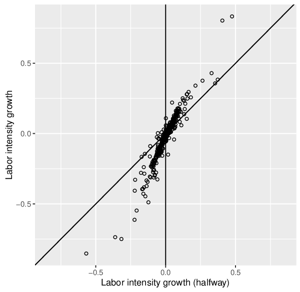
Let us consider the following labor intensity growth between the two periods $t=0,1$ for the $j$th sector:

Our database allows us to calculate labor intensity $a_{Ljt}=({w_{t}L_{jt}})/({p_{jt}Y_{jt})}$ for all $j$ sectors. However, they are also replicable by the system of unit cost functions $\bm{C}$ with restoring parameters as indicated in (42–43). We may then consider the following halfway labor intensity growth:

where ${a}_{Lj0.5}$ is obtained by the following calculations:

Here, sectoral TFP and primary factor prices are at halfway, i.e., $r_{0.5}=\frac{r_{1}+r_{0}}{2}$, $w_{0.5}=\frac{w_{1}+w_{0}}{2}$, and $\theta_{j0.5}=\frac{\theta_{j1}+\theta_{j0}}{2}$. Halfway commodity equilibrium price $\bm{p}_{0.5}$ is obtained by feedback recursion. Figure 6 displays sectoral labor intensity growth. Figure 6 displays halfway labor intensity growth on the horizontal axis.

We now consider an immortal representative household with identical $N$-commodity CES utility function $U(H_{1},\cdots,H_{N})$ of constant returns to scale, as follows:

where $0<\beta<1$ denotes the discount (time preference) factor. Elasticity of substitution, denoted as $1-\lambda$, is common across all goods. The share parameter $\mu_{i}$ must add up to one. Here, we assume that total labor supply $\mathcal{L}_{t}=\sum_{j=1}^{N}L_{jt}$ is determined by the demand side for all $t$, and not included in the utility function. Below is the representative household’s budget constraints:

We denote the ratio between capital stock and capital service by $\rho$ so that $\rho\mathcal{K}$ designates capital stock total when $\mathcal{K}$ denotes capital service total. Accordingly, $s$ denotes the price of capital. The depreciation rate is denoted by ${\delta}$. We use $\mathcal{B}$ to denote consumption expenditure total and $\mathcal{R}$ to denote the net export total. Regarding the linked input–output tables (2), (51) describes an equivalence between total expenditures and income of a representative household with the following: $\mathcal{B}_{t}=\sum_{i=1}^{N}p_{it}H_{it}$, $\mathcal{R}_{t}=\sum_{i=1}^{N}p_{it}E_{it}$, $\mathcal{L}_{t}=\sum_{j=1}^{N}L_{jt}$, $\mathcal{K}_{t}=\sum_{j=1}^{N}K_{jt}$, and $s_{t}(\rho\mathcal{K}_{t+1}-(1-\delta)\rho\mathcal{K}_{t})=\sum_{i=1}^{N}p_{it}G_{it}$.

Maximization of (50) subject to (51) yields the following Euler equation:

The CES indirect utility function must be of the following form:

Here, price index $I$ as defined above, is the cost of living index. We then know that the marginal utility of money can be expanded as follows:

Hence, by (52) and (54), the following condition must hold.

References

- Acemoglu and Guerrieri [2008] Acemoglu, D., Guerrieri, V., 2008. Capital deepening and nonbalanced economic growth. Journal of Political Economy 116, 467–498. doi:10.1086/589523.
- Alvarez-Cuadrado et al. [2018] Alvarez-Cuadrado, F., Long, N.V., Poschke, M., 2018. Capital-labor substitution, structural change and the labor income share. Journal of Economic Dynamics and Control 87, 206 – 231. doi:10.1016/j.jedc.2017.12.010.
- Antràs [2004] Antràs, P., 2004. Is the U.S. aggregate production function Cobb-Douglas? new estimates of the elasticity of substitution. Contributions in Macroeconomics 4, 67 – 69. doi:10.2202/1534-6005.1161.
- Arrow et al. [1961] Arrow, K.J., Chenery, H.B., Minhas, B.S., Solow, R.M., 1961. Capital-labor substitution and economic efficiencys. Review of Economics and Statistics 43, 225–250.
- Berndt [1976] Berndt, E.R., 1976. Reconciling alternative estimates of the elasticity of substitution. Review of Economics and Statistics 58, 59 – 68.
- Blackorby and Russell [1989] Blackorby, C., Russell, R.R., 1989. Will the real elasticity of substitution please stand up? (a comparison of the Allen/Uzawa and Morishima elasticities). American Economic Review 79, 882 – 888.
- Buera and Kaboski [2012] Buera, F.J., Kaboski, J.P., 2012. Scale and the origins of structural change. Journal of Economic Theory 147, 684 – 712. doi:10.1016/j.jet.2010.11.007. issue in honor of David Cass.
- Burfisher [2017] Burfisher, M.E., 2017. Introduction to Computable General Equilibrium Models. Cambridge University Press.
- Chenery and Watanabe [1958] Chenery, H.B., Watanabe, T., 1958. International comparisons of the structure of production. Econometrica 26, 487–521.
- Diewert [1976] Diewert, W.E., 1976. Exact and superlative index numbers. Journal of Econometrics 4, 115–145.
- Dixon and Jorgenson [2013] Dixon, P.B., Jorgenson, D.W. (Eds.), 2013. Handbook of Computable General Equilibrium Modeling. volume 1A of Handbooks in Economics. Elsevier, North Holland.
- Echevarria [2008] Echevarria, C., 2008. International trade and the sectoral composition of production. Review of Economic Dynamics 11, 192 – 206. doi:10.1016/j.red.2007.06.004.
- Herrendorf et al. [2015] Herrendorf, B., Herrington, C., Valentinyi, A., 2015. Sectoral technology and structural transformation. American Economic Journal: Macroeconomics 7, 104 – 133.
- Herrendorf et al. [2014] Herrendorf, B., Rogerson, R., Valentinyi, À., 2014. Chapter 6 - growth and structural transformation, in: Aghion, P., Durlauf, S.N. (Eds.), Handbook of Economic Growth. Elsevier. volume 2 of Handbook of Economic Growth, pp. 855 – 941. doi:10.1016/B978-0-444-53540-5.00006-9.
- Hudson and Jorgenson [1974] Hudson, E.A., Jorgenson, D., 1974. U.S. energy policy and economic growth, 1975-2000. Bell Journal of Economics 5, 461–514.
- Ida and Goto [2009] Ida, T., Goto, R., 2009. Simultaneous measurement of time and risk preferences: Stated preference discrete choice modeling analysis depending on smoking behavior. International Economic Review 50, 1169–1182. doi:10.1111/j.1468-2354.2009.00564.x.
- JIP [2015] JIP, 2015. Japan industrial productivity database. URL: http://www.rieti.go.jp/en/database/jip.html.
- Kawasaki et al. [2001] Kawasaki, K., Kumamoto, M., Ogawa, E., 2001. Empirical analysis on intrinsic bubbles in Japanese stock prices. The Hitotsubashi Review 126, 463–476. doi:10.15057/10342.
- Kim et al. [2017] Kim, J., Nakano, S., Nishimura, K., 2017. Multifactor CES general equilibrium: Models and applications. Economic Modelling 63, 115–127. doi:10.1016/j.econmod.2017.01.024.
- Klump and de La Grandville [2000] Klump, R., de La Grandville, O., 2000. Economic growth and the elasticity of substitution: Two theorems and some suggestions. American Economic Review 90, 282–291. doi:10.1257/aer.90.1.282.
- Klump et al. [2007] Klump, R., McAdam, P., Willman, A., 2007. Factor substitution and factor-augmenting technical progress in the United States: A normalized supply-side system approach. The Review of Economics and Statistics 89, 183–192. doi:10.1162/rest.89.1.183.
- Klump et al. [2012] Klump, R., McAdam, P., Willman, A., 2012. The normalized CES production function: Theory and empirics. Journal of Economic Surveys 26, 769–799. doi:10.1111/j.1467-6419.2012.00730.x.
- Kmenta [1967] Kmenta, J., 1967. On estimation of the CES production function. International Economic Review 8, 180–189.
- Krasnosel’skiĭ [1964] Krasnosel’skiĭ, M.A., 1964. Positive Solutions of Operator Equations. Groningen, P. Noordhoff.
- Matsuyama [2008] Matsuyama, K., 2008. Structural change, Palgrave Macmillan UK, London. The New Palgrave Dictionary of Economics, pp. 6408–6411. doi:10.1007/978-1-349-58802-2_1635.
- McFadden [1963] McFadden, D., 1963. Constant elasticity of substitution production functions. Review of Economic Studies 30, 73–83.
- MIAC [2016] MIAC, 2016. Ministry of Internal Affairs and Communications 2000–2005–2011 Linked Input-Output Tables [in Japanese]. URL: http://www.soumu.go.jp.
- Nakano and Nishimura [2018] Nakano, S., Nishimura, K., 2018. Structural propagation in a production network with restoring substitution elasticities. Physica A: Statistical Mechanics and its Applications 512, 986 – 999. doi:10.1016/j.physa.2018.08.110.
- Ngai and Pissarides [2007] Ngai, L.R., Pissarides, C.A., 2007. Structural change in a multisector model of growth. American Economic Review 97, 429 – 443.
- Nomura and Suga [2018] Nomura, K., Suga, Y., 2018. Measurement of depreciation rates using microdata from disposal survey of Japan, in: The 35th IARIW General Conference, Copenhagen, Denmark.
- Sato [1967] Sato, K., 1967. A two level constant elasticity of substitution production function. Review of Economic Studies 34, 116–138.
- Uzawa [1962] Uzawa, H., 1962. Production functions with constant elasticities of substitution. Review of Economic Studies 29, 291–299.
- Šizling and Storch [2004] Šizling, A.L., Storch, D., 2004. Power-law species-area relationships and self-similar species distributions within finite areas. Ecology Letters 7, 60–68. doi:10.1046/j.1461-0248.2003.00549.x.