Quantum spiral spin-tensor magnetism
Abstract
The characterization of quantum magnetism in a large spin () system naturally involves both spin-vectors and -tensors. While certain types of spin-vector (e.g., ferromagnetic, spiral) and spin-tensor (e.g., nematic in frustrated lattices) orders have been investigated separately, the coexistence and correlation between them have not been well explored. Here we propose a novel quantum spiral spin-tensor order on a spin-1 Heisenberg chain subject to a spiral spin-tensor Zeeman field, which can be experimentally realized using a Raman-dressed cold atom optical lattice. We develop a method to fully characterize quantum phases of such spiral tensor magnetism with the coexistence of spin-vector and spin-tensor orders as well as their correlations using eight geometric parameters. Our method provides a powerful tool for characterizing spin-1 quantum magnetism and opens an avenue for exploring novel magnetic orders and spin-tensor electronics/atomtronics in large-spin systems.
Introduction.— Quantum magnetism originates from the exchange coupling between quantum spins and lies at the heart of many fundamental phenomena in quantum physics Auerbach-1994; Schollwock-2008; Sachdev-2008. In particular, understanding exotic magnetic orders of strongly correlated quantum spin chains is one major issue of modern condensed matter physics. Such interacting many-body systems can give rise to various magnetic orders and the phase transitions between them DM-1; DM-2; Manousakis-1991; Haldane-1983; Affleck-1987; AKLT-1987; Islam2013; random2017. Major research efforts have been focused on spin-1/2 systems, where collinear (e.g., ferromagnetic and antiferromagnetic) and non-collinear (e.g., spiral) magnetic orders are fully characterized by the spin-vector () configurations, including their local orientations and densities as well as nonlocal correlations Greiner2011; Esslinger2013; Hulet2015; Bloch2016; Greiner2016; Greiner2017; wu2012; wu2013; wu2017; wu2018; Bloch2019.
Quantum magnetism with large spins, such as spin-1, has also received considerable attention in recent years, where the large spin could originate from, for instance, intrinsic orbital degrees of electrons or pseudo-spins defined by hyperfine states of cold neutral atoms or ions White-1993; Ripoll-2004; Rizzi-2005; Pixley2017; Pixley2018; Natu2015; spin-1SOC2016; Piraud2014; Hamley2012; Ueda2013; SOC-1BEC1; ions1. Mathematically, a full description of a large spin () involves not only rank-1 spin-vectors, but also higher-rank spin-tensors, therefore it is expected that the resulting quantum magnetism may possess both spin-vector and tensor orders. So far, spin-vector magnetism of a strongly correlated spin-1 (or higher) chain has been extensively studied Lou1999; Lou2005; Hagiwara2005; Manmana2011; Chiara2011; Rodriguez2011; Weyrauch2017; Pixley2017; Hermele2009; Gorshkov2010; Manmana2011A; yan2013; zhang2014, and the competition between spin interaction and Zeeman field (either uniform or spiral along the chain) leads to rich phase diagrams. Certain nematic magnetic orders of spin-tensors (with vanishing spin-vector) have been investigated in 2-dimensional (D) geometrically frustrated (e.g., triangle) lattices triangular1; triangular2; triangular3; triangular4; triangular5; triangular6; triangular7; triangular8; triangular9. However, magnetic orders with the coexistence of these two orders have not been discovered and a unified description of such magnetic orders is still lacking. Addressing these two important issues should be of great importance for the discovery of novel magnetic orders and the exploration of electronics/atomtronics characterized by spin-tensors.
We restrict to spin-1 magnetic orders, which may be characterized by two elements: rank-1 spin-vector (represented by an arrow using 3 parameters) and rank-2 spin-tensor (represented by an ellipsoid using 5 parameters). In this Letter, we propose a novel type of quantum spiral spin-tensor orders with the coexistence of spin-vector and tensor orders and develop a geometric method to describe them. Our main results are:
i) We propose an experimental setup for realizing a spin-1 Heisenberg chain subject to a spiral spin-tensor Zeeman field using a Raman coupled cold atom optical lattice, which can host the novel quantum spiral spin-tensor orders.
ii) We develop a method for characterizing any spin-1 quantum magnetism with the order parameters and long-range spin correlations described by eight geometric parameters originating from spin arrow and ellipsoid.
iii) We obtain the ground-state phase diagram numerically using the density-matrix renormalization group (DMRG) method and showcases its rich physics such as a ferromagnetic spiral tensor phase, where the relative orientation between spin-vector arrow and spin-tensor ellipsoid exhibits periodic oscillations. In previously studied spiral spin-vector order Pixley2017, arrow length, ellipsoid size, and their relative orientations are uniformly fixed across the lattice chain, while the 2D nematic phase in a frustrated lattice triangular1; triangular2 possesses vanishing spin-vector arrow and fixed ellipsoid size and directions.

The model.— We consider an experimental setup based on ultracold bosonic atoms in a 1D optical lattice, as shown in Fig. 1(a). Three Raman lasers are used to couple different spin and momentum states Ueda2013; Dalibard2011; Goldman2014; spielman2011; spielman2013; Zhai2015; Luo2017,. In particular, a pair of counter-propagating lasers with wavelength is used to realize the 1D optical lattice along the -direction, with wavenumber . All Raman lasers have an angle with respect to the -direction and they induce two Raman transitions between the spin states and [as shown in Fig. 1(b)] with the momentum transfer , where with the Raman-laser wavelength. Such Raman laser setup induces the spin-tensor-momentum coupling Luo2017 for ultra-cold atomic gases, which has been realized in experiment recently Li2020.
The tight-binding Hamiltonian without Raman lasers can be written as , where () is the creation (annihilation) operator with a spin , is the density operator, and with represent the total angular momentum spin operators and . is the tunneling amplitude between neighboring sites, and and are on-site density and spin interaction strengths.
In the Mott limit of commensurate odd integer filling and , we can get the effective spin Hamiltonian (see Appendix A), . Typically, for repulsive interaction, therefore we parameterize and on a unit circle with and and focus on the parameter region . For (i.e., ), the system possesses the ferromagnetic order, which maximizes but minimizes due to dominating negative bilinear interaction . For large negative biquadratic interaction in the region , the ground state should maximize by forming spin singlet between neighboring sites, which breaks the translational symmetry, leading to the dimer phase White-1993; Rizzi-2005; Ripoll-2004; Dimer2003. Typical values for alkaline atoms are for 23Na, for 7Li, for 41K, and for 87Rb Ueda2013.
The Raman lasers give rise to the site-dependent spin flipping terms and [see Fig. 1(c)], which would induce a spiral on-site spin-vector and tensor field. To see this, we write down the tight-binding Hamiltonian for such Raman processes , is the Raman coupling strength, describes the flux and can be tuned by the angle . In the Mott limit, can be treated as spiral spin-vector and spin-tensor Zeeman fields , where with the anticommutation relation and , is the Zeeman field strength, and is the spiral period of the field. The total Hamiltonian of our system reads
| (1) |
The competition between spin interaction and spiral on-site field may induce many novel spin-tensor magnetic phases, where both spin-vector and spin-tensor have to be considered to fully describe these quantum magnetic orders.

Description of spin-1 magnetic order.— The local magnetic order of a spin-1 system can be described by the local densities of 8 spin-moments (i.e., 3 spin-vectors and 5 spin-tensors). Here we consider the local spin-vector and the spin-tensor fluctuation matrix whose elements are tensor moments . Geometrically, is characterized by an arrow and by an ellipsoid (with principle axis lengths () and orientations given by the square-roots of the eigenvalues and eigenvectors of Bharath). To quantitatively characterize and geometrically visualize the magnetic order, we choose 8 independent geometric parameters that could fully describe the spin arrow and ellipsoid: the length and spherical coordinates , of the arrow, the two axis lengths with the third axis length and orientational Euler angles , , of the ellipsoid, as shown in Fig. 2(a).
Beside the local densities, the characterization of long-range correlations of the magnetic order requires spin-vector and spin-tensor correlations. In our Heisenberg model, only the same-spin-moment correlations are relevant because of the same-spin-moment interactions, and correlation function of spin moment over a distance can be defined as , with the average value of the -fold degenerate ground-states. The correlations can have the same geometrical representation as the local densities. The spin-vector correlation is described by an arrow with and spin arrow lengths , while the spin-tensor correlation is described by an ellipsoid with the principle axis lengths given by the tensor-correlation matrix .
Spiral spin-tensor magnetism.— The numerical ground-state phase diagram of the Hamiltonian (1) can be obtained through the DMRG calculation DMRG-1; DMRG-2, where the length of the spin chain is up to 96 sites, and we keep the maximum states at 200 and achieve truncation errors of . The resulting phase diagram for is plotted in the plane in Fig. 2(b). There are three different phases: the ferromagnetic spiral tensor phase (FST) for and the dimer spiral tensor phase (DST) for , both in the small spiral on-site field region, and the paramagnetic tensor phase (PT) for the large . All these phases possess both spiral spin-vector and -tensor densities and can be distinguished by spin correlations: i) For the FST phase, there are spin-vector and spin-tensor long-range correlations with nonzero ferromagnetic order ; ii) For the DST phase, the dimer-vector and dimer-tensor correlations are long-range with nonzero dimer order (see Appendix D); iii) For the PT phase, there is no any long-range correlations. For other spiral period , quantum phase diagrams are similar, except that the phase transitions may occur at different critical points and the period of the spiral modulation varies in the same way as the spiral period .
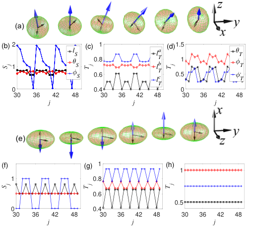
First we consider the region with the weak (the bottom-left part in the phase diagram), where the spin interactions are still dominant and the ferromagnetic order remains. At , the spin-vector arrow points to certain direction (assumed to be the axis) that does not change along the chain, and the spin-tensor ellipsoid is a flat disk in the - plane [i.e., , (i.e., axis is parallel to axis)] (see Appendix B). In the presence of the spiral Zeeman field (), the spin-vector density arrows , the spin-tensor density ellipsoids , and their relative orientations become oscillating periodically along the chain, forming spiral loops in the Bloch sphere (see Appendix B) and leading to the FST phase, where the local spiral magnetism and long-range correlations coexist. Fig. 3(a) shows the arrows and ellipsoids in one spatial period, which possess spiral structure.
For the quantitative characterization of the spiral tensor order, we plot the spatial distributions of for the vector-density arrows, the principle axis lengths , and the orientational Euler angles of the ellipsoids in Figs. 3(b)-3(d). We find , and oscillate along the chain with the period same as the spiral field, and changes from to during one period [see Fig. 3(b)]. Correspondingly, the arrows within one period form a circular loop around the axis (see Appendix B). For the spin-tensor density ellipsoids , beside the modulation in its size [see Fig. 3(c)], the corresponding axes form a twisted loop (-shaped) (see Appendix B), leading to relative rotations between spin-vector density arrows and spin-tensor density ellipsoids [, and oscillate differently from , ], as shown in Fig. 3(d). Such spiral magnetic configuration originates from the competition between the on-site spin-vector potential [] and spin-tensor potential []. Without the spin-tensor field (i.e. only spin-vector field), the spin-vector density arrows and spin-tensor density ellipsoids would rotate similarly with fixed relative orientation [i.e., , and uniform along the chain], and all ellipsoids would have a fixed size [i.e., uniform along the chain] (see Appendix C). Moreover, the ferromagnetic spiral order is characterized by the long-range correlation of both spin-vector and spin-tensor (see Appendix B).
As we increase , the spin-vector rotation loop in a period first enlarges and then shrinks to a narrow ellipse (cigar-shaped). For a strong , the system undergoes a second-order phase transition from the FST phase to the PT phase, where the long-range correlations and ferromagnetic order vanish [see Fig. 4(c)]. In the PT phase, the on-site Zeeman field in Hamiltonian (1) dominates, and all spin-vector density arrows are parallel to the Zeeman field [] with length modulations. The corresponding local magnetic densities are shown in Fig. 3(e). Clearly, the spin-vector density loop shrinks into a line on the -axis in the PT phase ( and ).
The rotation loop of the tensor ellipsoids changes similarly as we increase : the loop first enlarges then shrinks into a line after the phase transition, where only the sizes (not the direction) of the ellipsoids oscillate (see Appendix B), as shown in Figs. 3(g) and 3(h). The oscillation of makes the PT phase different from regular paramagnetic phase. In the PT phase, the vector correlation arrows and tensor correlation ellipsoids decay exponentially (in size) with the distance , indicating that there does not exist any long-range order (see Appendix B).
Now we turn to the parameter region . The system still stays in the PT phase for a large . For a small , the negative biquadratic interaction dominates, leading to the second-order phase transition to the DST phase. In this phase, the local spin-vector and spin-tensor densities behave similarly as in the PT phase, forming lines instead of spiral loops (see Appendix B). Interestingly, there exist spiral loops for the dimer-vector densities and dimer-tensor densities (see Appendix D), thanks to the presence of the on-site spin-tensor field. The ordinary correlations of both spin-vector and spin-tensor decay similarly as the PT phase (see Appendix D). However, there exist long-range correlations for both dimer-vector and dimer-tensor (see Appendix D), and the dimer order emerges.
Phase transitions.— The phase transitions between above phases can be characterized by the critical behaviors of the local densities and the correlations of the spin-vectors and -tensors. When increases from zero, the spiral loops of spin-vector density arrows and spin-tensor density ellipsoids’ axes emerge from initial uniform distribution, become larger, then shrink, and finally disappear at the phase transition (see Appendix B). The spin-tensor density ellipsoids have two critical behaviors when crossing the phase transition: i) the angles shows a large oscillation in the real space, which can be characterized by a sharp peak for the oscillatory amplitude of angles located at the phase boundary, as clearly shown in Fig. 4(a); ii) the oscillatory amplitude of ellipsoid’s axis lengths have sharp features at the critical point, as shown in Fig. 4(b). In addition, the ferromagnetic order decreases and vanishes across the phase transition, as shown in Fig. 4(c).
The transition from the PT to FST or DST phases corresponds to the formation of the long-range order, therefore the transition should also be captured by more essential correlation lengths. The numerical results for the spin-vector (-tensor) correlation length Campostrini2014 () for the transition between PT and FST phases are shown in Fig. 4(d), which show that there are (no) spin-vector and -tensor long-range correlations for the FST (PT) phase. The critical point in the thermodynamic limit is determined by the crossing point between curves for different finite lattice lengths, as shown in Fig. 4(d).
Similarly, Figs. 4(e) and 4(f) show the dimer order and dimer-vector(-tensor) correlation length for finite lattice lengths, where () is used to determine the critical point between PT and DST phases. The dimer correlation length of a finite lattice length retains and then decays. In the decaying region, the dimer correlation lengths of several finite lattices cross at one point. In the process of increasing , the dimer-vector(-tensor) density spiral loop emerges from a uniform distribution, becomes larger, then shrinks, and finally disappears (see Appendix D).
Discussion and conclusions.— The phase transition is related with the symmetry of the Hamiltonian. For instance, in the FST phase, the ground state is 4-fold degenerate due to spontaneously symmetry breaking of the exchange symmetry and reflection symmetry of the Hamiltonian (1), leading to nonzero and . However, in the PT phase, the ground state is non-degenerate, yielding and , thus the spiral loop shrinks into a line ( oscillate, , ) [see Fig. 3(f)].
Finally we remark that the local spin states are mixed states for the strongly correlated spin chain, therefore another useful representation of higher-spin pure states, Majorana stars Ueda2013; Majorana1932; Majorana1998; Majorana2012; Majorana2013zhai; Majorana2014, is not suitable for studying correlated quantum magnetism. The spin-tensor can appear not only as an on-site Zeeman field, but also as interactions between nearest-neighbor sites. We show the magnetic order with spin-tensor interaction in Appendix F.
In summary, we propose a new type of quantum magnetism, the spiral spin-tensor order, in a spin-1 Heisenberg chain subject to a spiral spin-tensor Zeeman field. We characterize such quantum spiral spin-tensor orders and their phase transitions using local spin-vector and -tensor densities and their correlations, which can be visualized using eight geometric parameters. To detect such magnetic orders, we can isolate the sites of interest using additional site-resolved potentials and measure their local spin states and non-local spin correlations Greiner2011; Greiner2016; Greiner2017; Bloch2016. Our method can also be used to describe spin-1 quantum magnetism formed by trapped ion array with tunable long-range interactions ions1. Our work should lay the foundation for exploring strongly-correlated quantum magnetism in a large spin system and pave the way for engineering novel types of spin-tensor electronic/atomtronic devices.
Acknowledgements.
Acknowledgements: X. Z., G. C., and S. J. are supported by National Key R&D Program of China under Grants No. 2017YFA0304203; the NSFC under Grants No. 11674200 and No. 11804204; and 1331KYC. X. L. and C. Z. are supported by AFOSR (FA9550-16-1-0387), ARO (W911NF-17-1-0128), and NSF (PHY-1806227),Appendix A Derivation of Hamiltonian (1)
The tight-binding Hamiltonian (1) can be written as three terms
| (2) |
where
| (3) | |||||
| (4) | |||||
| (5) |
The effective spin model is obtained through the projection
| (6) |
where is the projection operator that projects the states into the low-energy subspace with a filling ( is an odd integer), is the Hamiltonian after the Schrieffer-Wolff transformation Schrieffer-Wolff
| (7) | |||||
In the Mott insulator region, the hopping term is small. We choose such that , thus
| (8) | |||||
Up to the second order of ( is the first order), we have
| (9) |
Denote as the projection operator that projects the states into the subspace of the high-energy with filling. Because , we have
| (10) | |||||
where, . is not affected by . Thus the effective spin Hamiltonian
| (11) | |||||
where, , ,
Here and are given by Imambekov-2003
, and . After ignoring the constant term, the final effective spin Hamiltonian becomes,
| (12) | |||||
Appendix B Spin-vector and spin-tensor magnetic orders

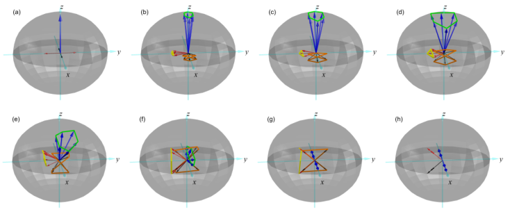
Without the on-site Zeeman field (), the ferromagnetic spiral tensor (FST) phase reduces to the ordinary ferromagnetic phase (F). The corresponding local magnetic orders represented by the spin-vector density arrows and spin-tensor density ellipsoids’ axes are uniform in space, as shown in Fig. 5(a). For the FST with a small , the spin-vector density arrows and spin-tensor density ellipsoids’ axes oscillate along the spin chain, forming spiral loops, as shown in Fig. 5(b). With increasing , the spiral loops first enlarge [see Figs. 5(c)-5(d)], then shrink to a narrow ellipse [see Figs. 5(e)-5(g)]. Across the phase transition point to the paramagnetic tensor phase (PT), the loops shrink to lines, where the spin-vector density arrows become parallel to the Zeeman field direction [see Fig. 5(h)].
With increasing , the relative rotation between two neighboring ellipsoids’ axes becomes more significant [see Fig. 3(a) in the main text]. In the paramagnetic tensor phase, the relative rotation angle becomes [see Fig. 3(e) in the main text]. Both the size and orientation of the ellipsoids oscillate along the spin chain, and a orientation change is equivalent to a size deformation without rotation. Therefore in the paramagnetic tensor phase, we only have the modulation in the ellipsoid size [see Fig. 3(e) in the main text].
The ferromagnetic spiral order is characterized by the long-range correlation of both spin-vector and spin-tensor . The spin arrow lengths and axis lengths of ellipsoids exhibit power-low decay with the distance , as shown in Figs. 6(a) and 6(b). In the paramagnetic tensor phase, the vector correlation arrows and tensor correlation ellipsoids decrease ( and exhibit exponential decay) with the distance , indicating that there is no long-range order, as shown in Figs. 6(c) and 6(d).

Appendix C The results due to the spin-vector potential
In contrast, in the ferromagnetic spiral vector phase induced by spiral spin-vector Zeeman field in previous studies Pixley2017 (tensor results were not discussed in these works), the spin-vector density arrows and spin-tensor density ellipsoids would rotate similarly with fixed relative orientation [i.e. , and are uniform along the chain], and all ellipsoids have fixed sizes [i.e. uniform along the chain], as shown in Fig. 7.
Appendix D Dimer spiral tensor phase



The spin-1 Hamiltonian may support dimer orders in certain parameter region (i.e. ), which describe the pairing order between two neighboring sites. The corresponding dimer-vector and dimer-tensor operators are defined as and . For instance, the dimer-vector and dimer-tensor are nonzero for the spin singlet pairing between neighboring sites in the dimer phase for the Hamiltonian even without the spiral Zeeman field. Such dimer-vector density and dimer-tensor density can also be described geometrically using arrows and ellipsoids, similar as the spin-vector and spin-tensor for a single site. There are also 8 dimer-moments (i.e., 3 dimer-vectors and 5 dimer-tensors: the length and spherical coordinates , of the arrow, the two axis lengths with the third axis length and orientational Euler angles , , of the ellipsoid). Similarly, dimer-vector correlation with elements can be described by arrows with the length of arrows, and dimer-tensor correlation can be described by ellipsoids with principle axis lengths () given by the matrix , respectively.
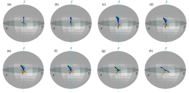
The dimer spiral tensor phase (DST) is non-degenerate, therefore the behaviors of spin-vector arrows and spin-tensor ellipsoids are the same as those in the paramagnetic tensor phase [see Fig. 8(a)]. Only the spin-tensor density ellipsoid’s lengths oscillate, while the angles , and are uniform. Specifically, the size of spin-vector density arrows and spin-tensor density ellipsoids oscillate along the chain, forming lines in the Bloch sphere that are similar as those for the paramagnetic tensor phase [see Figs. 8(b)-8(d)]. However, the dimer-vector density and dimer-tensor density can form spiral loops for a finite , as shown in Fig. 8(e). The , and oscillate along the chain [see Fig. 8(f)]. The dimer-tensor ellipsoids’ lengths and Euler angles , , oscillate along the chain [, oscillate differently from , ] [see Figs. 8(g) and 8(h)], originating from different spiral loops for the dimer-vector arrows and the dimer-tensor ellipsoid .
For the ordinary dimer phase (D) with , the dimer-vector density arrows and dimer-tensor density ellipsoids’ axes are uniform in space, as shown in Fig. 9(a). In the dimer spiral tensor phase with increasing , the spiral loop for the dimer order first enlarges [see Figs. 9(b)-9(g)], then shrinks into a point at the phase transition to the paramagnetic tensor phase [see Fig. 9(h)]. For the on-site Zeeman field given in the main text, the system has a mirror symmetry, therefore the spiral loops formed by the dimer densities shrink to lines. If a phase shift between spin-vector and -tensor terms is introduced to the on-site Zeeman field modulation along the chain, the mirror symmetry is broken and the dimer spiral loops would emerge as circles. In addition, the dimer-vector density and dimer-tensor density form different spiral loops, leading to relative rotations between them, as shown in Fig. 10.
There is no long-range ordinary correlations of spin-vector and spin-tensor in the dimer spiral tensor phase [see Figs. 11(a) and 11(b)], which are the same as the paramagnetic tensor phase [see Figs. 6(c) and 6(d)]. Instead, the system possesses long-range dimer correlations for both dimer-vector and dimer-tensor , the length of arrows and the axes length of ellipsoids () exhibit power-low decay and have long-range correlations [see Figs. 11(c) and 11(d)].
Appendix E Correlation lengths near phase transitions
The critical point for the phase transition between ferromagnetic spiral tensor and paramagnetic tensor phases in the thermodynamic limit can be examined by the spin-vector(-tensor) correlation lengths (). The DMRG results show that for several finite lattice lengths cross at one point with increasing , which is the critical point between ferromagnetic spiral tensor and paramagnetic tensor phases, as shown in Fig. 12.
Similarly, the phase transition between dimer spiral tensor and paramagnetic tensor phases in the thermodynamic limit can be examined by the dimer-vector(-tensor) correlation lengths (). There is (no) long-range dimer correlation in the thermodynamic limit for the dimer spiral tensor (paramagnetic tensor) phase. With increasing , the dimer correlation length for a finite lattice retains and then decays. In the decay region, for several finite lattice lengths cross at one point, which corresponds to the phase transition critical point , as shown in Fig. 13.
Appendix F Magnetic order with spin-tensor interaction
The spin-tensor can appear not only as an on-site Zeeman field, but also as interactions between nearest-neighbor sites. The biquadratic term of Hamiltonian (1) in the main text contains many types of spin-tensor interactions, making it hard to identify the spin-tensor correlations induced by each term. Moreover, the spin-tensor correlations cannot be isolated out because they are bound with the spin-vector correlations. Here we consider a simple toy spin Hamiltonian,
| (13) | |||||
where and . The competition between the spin-vector and spin-tensor interactions induces ferromagnetic or antiferromagnetic vector or tensor phases for different , as shown in Fig. 14.
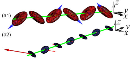
A weak spiral zeeman field (here we take ) can induce spiral spin-vector densities, but does not affect the long-range magnetic order. We find that the ferromagnetic (antiferromagnetic) vector phases are similar as those discussed in Ref. Pixley2017, where the system possesses both long-range vector and tensor correlations with spiral spin-vectors densities, and the long-range tensor correlations are induced by the spin-vector interactions. In ferromagnetic (antiferromagnetic) tensor phase [FT (AFT)], the system only possesses long-range spin-tensor correlations (with no long-range spin-vector correlations), which are induced directly by the spin-tensor interactions. In the AFT phase, the spin-tensor density ellipsoids have orthogonal axes between nearest-neighbor sites, while in the FT phase, the axes of the ellipsoids are parallel between nearest-neighbor sites. In both the FT and AFT phases, the spin-vector density arrows are spiral along the chain. Such FT and AFT phases due to the spin-tensor interactions are very different from previous studies of spin-vector interactions. As examples, in Figs. 15(a1)-15(a2), we show the magnetic local densities and non-local correlations in the AFT phase.
References
- (1) A. Auerbach, Interacting electrons and quantum magnetism (Springer, New York, 1994).
- (2) U. Schollwöck, J. Richter, D. J. J. Farnell, and R. F. Bisho, Quantum magnetism (Springer, New York, 2008).
- (3) S. Sachdev, Quantum magnetism and criticality, Nat. Phys. 4, 173 (2008).
- (4) I. Dzyaloshinskii, A thermodynamic theory of weak ferromagnetism of antiferromagnetics, J. Phys. Chem. Solids 4, 241 (1958).
- (5) T. Moriya, Anisotropic superexchange interaction and weak ferromagnetism, Phys. Rev. 120, 91 (1960).
- (6) E. Manousakis, The spin-1/2 Heisenberg antiferromagnet on a square lattice and its application to the cuprous oxides. Rev. Mod. Phys. 63, 1 (1991).
- (7) F. D. M. Haldane, Nonlinear field theory of large-spin heisenberg antiferromagnets: Semiclassically quantized solitons of the one-dimensional easy-axis néel state, Phys. Rev. Lett. 50, 1153 (1983).
- (8) I. Affleck and F. D. M. Haldane, Critical theory of quantum spin chains, Phys. Rev. B 36, 5291(1987).
- (9) I. Affleck, T. Kennedy, E. H. Lieb, and H. Tasaki, Rigorous results on valence-bond ground states in antiferromagnets, Phys. Rev. Lett. 59, 799 (1987).
- (10) R. Islam, C. Senko, W. C. Campbell, S. Korenblit, J. Smith, A. Lee, E. E. Edwards, C.-C. J. Wang, J. K. Freericks, and C. Monroe, Emergence and frustration of magnetic order with variable-range interactions in a rrapped ion quantum simulator, Science 340, 583 (2013).
- (11) K. D. McAlpine, S. Paganelli, S. Ciuchi, A. Sanpera, and G. D. Chiara, Magnetic phases of spin-1 lattice gases with random interactions, Phys. Rev. B 95, 235128 (2017).
- (12) J. Simon, W. S. Bakr, R. Ma, M. E. Tai, P. M. Preiss, and M. Greiner, Quantum simulation of antiferromagnetic spin chains in an optical lattice, Nature (London) 472, 307 (2011).
- (13) M. F. Parsons, A. Mazurenko, C. S. Chiu, G. Ji, D. Greif, and M. Greiner, Site-resolved measurement of the spin-correlation function in the Fermi-Hubbard model, Science 353, 1253 (2016).
- (14) A. Mazurenko, C. S. Chiu, G. Ji, M. F. Parsons, M. Kanász-Nagy, R. Schmidt, F. Grusdt, E. Demler, D. Greif, and M. Greiner, A cold-atom Fermi-Hubbard antiferromagnet, Nature (London) 545, 462 (2017).
- (15) M. Boll, T. A. Hilker, G. Salomon, A. Omran, J. Nespolo, L. Pollet, I. Bloch, and C. Gross, Spin- and density-resolved microscopy of antiferromagnetic correlations in Fermi-Hubbard chains. Science 353, 1257 (2016).
- (16) D. Greif, T. Uehlinger, G. Jotzu, L. Tarruell, and T. Esslinger, Short-range quantum magnetism of ultracold fermions in an optical lattice, Science 340, 1307 (2013).
- (17) R. A. Hart, P. M. Duarte, T.-L. Yang, X. Liu, T. Paiva, E. Khatami, R. T. Scalettar, N. Trivedi, D. A. Huse, and R. G. Hulet, Observation of antiferromagnetic correlations in the Hubbard model with ultracold atoms, Nature (London) 519, 211 (2015).
- (18) Z. Cai, X. Zhou, and C. Wu, Magnetic phases of bosons with synthetic spin-orbit coupling in optical lattices, Phys. Rev. A 85, 061605 (2012).
- (19) Z. Cai, H. Hung, L. Wang, and C. Wu, Quantum magnetic properties of the SU(2N) Hubbard model in the square lattice: a quantum Monte Carlo study, Phys. Rev. B 88, 125108 (2013).
- (20) W. Yang, J. Wu, S. Xu, Z. Wang, and C. Wu, Quantum spin dynamics of the axial antiferromagnetic spin-1/2 XXZ chain in a longitudinal magnetic field, arXiv:1702.01854
- (21) Z. Wang, J. Wu, W. Yang, A. K. Bera, D. Kamenskyi, A. T. M. N. Islam, S. Xu, J. M. Law, B. Lake, C. Wu, and A. Loidl, Experimental observation of bethe strings, Nature (London) 554, 219 (2018).
- (22) G. Salomon, J. Koepsell, J. Vijayan, T. A. Hilker, J. Nespolo, L. Pollet, I. Bloch, and C. Gross, Direct observation of incommensurate magnetism in Hubbard chains, Nature (London) 565, 56 (2019).
- (23) S. R. White and D. A. Huse, Numerical renormalization-group study of low-lying eigenstates of the antiferromagnetic S=1 heisenberg chain, Phys. Rev. B 48, 3844 (1993).
- (24) J. J. García-Ripoll, M. A. Martin-Delgado, and J. I. Cirac, Implementation of spin Hamiltonians in optical lattices, Phys. Rev. Lett. 93, 250405 (2004)
- (25) M. Rizzi, D. Rossini, G. De Chiara, S. Montangero, and R. Fazio, Phase diagram of spin-1 bosons on one-dimensional lattices, Phys. Rev. Lett. 95, 240404 (2005).
- (26) C. D. Hamley, C. S. Gerving, T. M. Hoang, E. M. Bookjans, and M. S. Chapman, Spin-nematic squeezed vacuum in a quantum gas, Nat. Phys. 8, 305 (2012).
- (27) D. M. Stamper-Kurn and M. Ueda, Spinor Bose gases: Symmetries, magnetism, and quantum dynamics, Rev. Mod. Phys. 85, 1191 (2013).
- (28) M. Piraud, Z. Cai, I. P. McCulloch, and U. Schollwöck, Quantum magnetism of bosons with synthetic gauge fields in one dimensional optical lattices: A density-matrix renormalizationgroup study, Phys. Rev. A 89, 063618 (2014).
- (29) S. S. Natu, X. Li, and W. S. Cole, Striped ferronamatic ground states in a spin-orbit-coupled S=1 Bose gas, Phys. Rev. A 91, 023608 (2015).
- (30) D. Campbell, R. Price, A. Putra, A. Valdés-Curiel, D. Trypogeorgos, and I. B. Spielman, Magnetic phases of spin-1 spin-orbit-coupled Bose gases, Nat. Commun. 7, 10897 (2016).
- (31) G. Martone, F. Pepe, P. Facchi, S. Pascazio, and S. Stringari, Tricriticalities and quantum phases in spin-orbit-coupled spin-1 Bose gases, Phys. Rev. Lett. 117, 125301 (2016).
- (32) E. J. König and J. H. Pixley, Quantum field theory of nematic transitions in spin orbit coupled spin-1 polar bosons, Phys. Rev. Lett. 121, 083402 (2018).
- (33) C. Senko, P. Richerme, J. Smith, A. Lee, I. Cohen, A. Retzker, and C. Monroe, Realization of a Quantum Integer-Spin Chain with Controllable Interactions, Phys. Rev. X. 5, 021026 (2015).
- (34) J. H. Pixley, W. S. Cole, I. B. Spielman, M. Rizzi, and S. D. Sarma, Strong-coupling phases of the spin-orbit-coupled spin-1 Bose-Hubbard chain: Odd-integer Mott lobes and helical magnetic phases, Phys. Rev. A 96, 043622 (2017).
- (35) J. Lou, X. Dai, S. Qin, Z. Su, and L. Yu, Heisenberg spin-1 chain in a staggered magnetic field: A density-matrix-renormalization-group study, Phys. Rev. B 60, 52 (1999).
- (36) J. Lou, C. Chen, J. Zhao, X. Wang, T. Xiang, Z. Su, and L. Yu, Midgap states in antiferromagnetic Heisenberg chains with a staggered field, Phys. Rev. Lett. 94, 217207 (2005).
- (37) M. Hagiwara, L. P. Regnault, A. Zheludev, A. Stunault, N. Metoki, T. Suzuki, S. Suga, K. Kakurai, Y. Koike, P. Vorderwisch, and J.-H. Chung, Spin excitations in an anisotropic bond-alternating quantum S=1 chain in a magnetic field: Contrast to Haldane spin chains, Phys. Rev. Lett. 94, 177202 (2005).
- (38) S. R. Manmana, A. M. Läuchli, F. H. L. Essler, and F. Mila, Phase diagram and continuous pair-unbinding transition of the bilinear-biquadratic S=1 Heisenberg chain in a magnetic field, Phys. Rev. B 83, 184433 (2011).
- (39) G. D. Chiara, M. Lewenstein, and A. Sanpera, Bilinear-biquadratic spin-1 chain undergoing quadratic Zeeman effect, Phys. Rev. B 84, 054451 (2011).
- (40) K. Rodríguez, A. Argüelles, A. K. Kolezhuk, L. Santos, and T. Vekua, Field-Induced Phase Transitions of Repulsive Spin-1 Bosons in Optical Lattices, Phys. Rev. Lett. 106, 105302 (2011).
- (41) M. Weyrauch and M. V. Rakov, Dimerization in ultracold spinor gases with Zeeman splitting, Phys. Rev. B 96, 134404 (2017).
- (42) M. Hermele, V. Gurarie, and A. M. Rey, Mott Insulators of Ultracold Fermionic Alkaline Earth Atoms: Underconstrained Magnetism and Chiral Spin Liquid, Phys. Rev. Lett. 103, 135301 (2009).
- (43) A. V. Gorshkov, M. Hermele, V. Gurarie, C. Xu, P. S. Julienne, J. Ye, P. Zoller, E. Demler, M. D. Lukin, and A. M. Rey, Two-orbital SU(N) magnetism with ultracold alkaline-earth atoms, Nat. Phys. 6, 289 (2010).
- (44) S. R. Manmana, K. R. A. Hazzard, G. Chen, A. E. Feiguin, and A. M. Rey, SU(N) magnetism in chains of ultracold alkaline-earth-metal atoms: Mott transitions and quantum correlations, Phys. Rev. A 84, 043601 (2011).
- (45) B. Yan, S. A. Moses, B. Gadway, J. P. Covey, K. R. A. Hazzard, A. M. Rey, D. S. Jin, and J. Ye, Observation of dipolar spin-exchange interactions with lattice-confined polar molecules, Nature (London) 501, 521 (2013).
- (46) X. Zhang, M. Bishof, S. L. Bromley, C. V. Kraus, M. S. Safronova, P. Zoller, A. M. Rey, and J. Ye, Spectroscopic observation of SU(N)-symmetric interactions in Sr orbital magnetism. Science 345, 1467 (2014).
- (47) H. Tsunetsugu and M. Arikawa, Spin nematic phase in S=1 triangular antiferromagnets, J. Phys. Soc. Jpn. 75, 083701 (2006).
- (48) A. Läuchli, F. Mila, and K. Penc, Quadrupolar phases of the S=1 bilinear-biquadratic Heisenberg model on the triangular lattice, Phys. Rev. Lett. 97, 087205 (2006).
- (49) S. Bhattacharjee, V. B. Shenoy, and T. Senthil, Possible ferro-spin nematic order in NiGa2S4, Phys. Rev. B 74, 092406 (2006).
- (50) J.-H. Park, S. Onoda, N. Nagaosa, and J. H. Han, Nematic and chiral order for planar spins on a triangular lattice, Phys. Rev. Lett. 101, 167202 (2008)
- (51) R. K. Kaul, Spin nematic ground state of the triangular lattice S=1 biquadratic model, Phys. Rev. B 86, 104411 (2012).
- (52) C. Xu, F. Wang, Y. Qi, L. Balents, and M. P. A. Fisher, Spin liquid phases for spin-1 systems on the triangular lattice, Phys. Rev. Lett. 108, 087204 (2012).
- (53) T. A. Tóth, A. M. Läuchli, F. Mila, and K. Penc, Competition between two- and three-sublattice ordering for S=1 spins on the square lattice, Phys. Rev. B 85, 140403 (2012)
- (54) A. Smerald and N. Shannon, Theory of spin excitations in a quantum spin-nematic state, Phys. Rev. B 88, 184430 (2013).
- (55) R. Yu and Q. Si, Antiferroquadrupolar and Ising-Nematic Orders of a Frustrated Bilinear-Biquadratic Heisenberg Model and Implications for the Magnetism of FeSe, Phys. Rev. Lett. 115, 116401 (2015).
- (56) J. Dalibard, F. Gerbier, G. Juzeliūnas, and P. Öhberg, Colloquium: Artificial gauge potentials for neutral atoms, Rev. Mod. Phys. 83, 1523 (2011).
- (57) N. Goldman, G. Juzeliūnas, P. Öhberg, and I. B. Spielman, Light-induced gauge fields for ultracold atoms, Rep. Prog. Phys. 77, 126401 (2014).
- (58) Y.-J. Lin, K. Jiménez-García, and I. B. Spielman, Spin-orbit-coupled Bose-Einstein condensates, Nature (London) 471, 83 (2011).
- (59) V. Galitski and I. B. Spielman, Spin-orbit coupling in quantum gases, Nature (London) 494, 49 (2013).
- (60) H. Zhai, Degenerate quantum gases with spin-orbit coupling: A review, Rep. Prog. Phys. 78, 026001 (2015).
- (61) X.-W. Luo, K. Sun, and C. Zhang, Spin-tensor–momentum-coupled Bose-Einstein condensates, Phys. Rev. Lett. 119, 193001 (2017).
- (62) D. Li, L. Huang, P. Peng, G. Bian, P. Wang, Z. Meng, L. Chen, and J. Zhang, Experimental realization of a spin-tensor momentum coupling in ultracold Fermi gases, manuscript under review (2020).
- (63) S. K. Yip, Dimer state of spin-1 bosons in an optical lattice, Phys. Rev. Lett. 90, 250402 (2003).
- (64) H. M. Bharath, Non-abelian geometric phases carried by the spin fluctuation tensor, J. Math. Phys. 59, 062105 (2018).
- (65) S. R. White, Density matrix formulation for quantum renormalization groups, Phys. Rev. Lett. 69, 2863 (1992).
- (66) U. Schollwök, The density-matrix renormalization group, Rev. Mod. Phys. 77, 259 (2005).
- (67) M. Campostrini, A. Pelissetto, and E. Vicari, Finite-size scaling at quantum transitions, Phys. Rev. B 89, 094516 (2014).
- (68) E. Majorana, Atomi orientati in campo magnetico variabile, Nuovo Cimento 9, 43 (1932).
- (69) J. H. Hannay, The Berry Phase for Spin in the Majorana Representation, J. Phys. A 31, L53 (1998).
- (70) B. Lian, T.-L. Ho, and H. Zhai, Searching for non-Abelian phases in the Bose-Einstein condensate of dysprosium, Phys. Rev. A 85, 051606 (2012).
- (71) X. Cui, B. Lian, T.-L. Ho, B. L. Lev, and H. Zhai, Synthetic gauge field with highly magnetic lanthanide atoms, Phys. Rev. A 88, 011601 (2013).
- (72) H. D. Liu and L. B. Fu, Representation of Berry Phase by the Trajectories of Majorana Stars, Phys. Rev. Lett. 113, 240403 (2014).
- (73) J. R. Schrieffer and P. A.Wolff, Relation between the Anderson and Kondo Hamiltonians, Phys. Rev. 149, 491 (1966).
- (74) A. Imambekov, M. Lukin, and E. Demler, Spin-exchange interactions of spin-one bosons in optical lattices: Singlet, nematic, and dimerized phases, Phys. Rev. A 68, 063602 (2003).