Training Artificial Neural Networks by Generalized Likelihood Ratio Method: Exploring Brain-like Learning to Improve Robustness
Abstract
In this work, we propose a generalized likelihood ratio method capable of training the artificial neural networks with some biological brain-like mechanisms,.e.g., (a) learning by the loss value, (b) learning via neurons with discontinuous activation and loss functions. The traditional back propagation method cannot train the artificial neural networks with aforementioned brain-like learning mechanisms. Numerical results show that the robustness of various artificial neural networks trained by the new method is significantly improved when the input data is affected by both the natural noises and adversarial attacks. Code is available at: https://github.com/LX-doctorAI/GLR_ADV .
1 Introduction
Artificial neural network (ANN) has been used as a universal classifier. In recent years, there have been tremendous successes in applying ANNs to image processing, speech recognition, game, and medical diagnosis (He et al. 2016; Graves et al. 2013; Silver et al. 2016; Gulshan et al. 2016; Esteva et al. 2017) . In ANN, the inputs such as texts and images are turned into a vector, and each neuron performs a nonlinear transformation on the input vector. A deep learning ANN typically contains multiple layers of convoluted neurons. This complicated machinery maps the input space to the target space. There are synaptic weights in each neuron to be adapted to the surrounding environment based on the loss between the ANN output and target data. The back propagation (BP) method has been the most widely used technique to train ANNs. However, the BP method requires the loss function and activation function to be smooth in ANNs, which limits the capability of ANNs to fit well with the surrounding environments.
Recent work in deep learning has demonstrated that ANNs can be more easily confused by small noises added to the images via snowing, blurring, and pixelation than human being (Hendrycks & Dietterich 2018; Recht et al. 2018; Azulay & Weiss 2018; Dan et al. 2018). Moreover, ANNs are vulnerable to adversarial attacks, where a very small perturbation of the inputs can drastically alter the classification result (C. Szegedy & Fergus 2014; Goodfellow et al. 2014; Carlini & Wagner 2017; Seyed-Mohsen Moosavi-Dezfooli & Frossard 2016; Bastani et al. 2016). In contrast, the adversarial phenomenon rarely happens for human being (Elsayed et al. 2018).
Then some interesting questions arise: what are the differences between biological neural networks in the human brains and ANNs? Can we borrow some mechanisms from the biological brain neural networks to improve the robustness of ANNs? There are some noticeable differences between the neurons in human brain and the neurons used in traditional ANNs (Dayan & Abbott 2018). First, the activation of the brain neuron is via an electric impulse, which can be captured by a threshold activation function, and there exists a (neuronal) noise in each neuron, whereas the traditional ANN uses continuous activation functions, e.g., Sigmoid and ReLu, and a deterministic nonlinear transformation. Second, human brain perceives an object as a specific category, e.g., dog or cat, which means that the loss function capturing the mechanism of a human brain should be a discontinuous zero-one function, whereas the loss functions in ANNs are smooth, e,g., the cross-entropy function. Furthermore, the brain neuron network is effected directly by the electronic signal sent by a sensory system and the chemical signal from the endocrine, therefore the biological brain functions like learning from the loss value itself rather than the gradient of the loss, which the BP method uses.
In this work, a generalized likelihood ratio (GLR) method is proposed to train ANNs with neuronal noises. Unlike the BP method, GLR trains ANNs directly by the loss value, rather than the gradient of the loss. GLR does not differentiate the sample path of the loss, and it can train ANNs with discontinuous activation and loss functions. Therefore, the new training method generalizes the scope of ANNs to be used in practice, which allows some brain-like mechanisms, i.e., (a) learning by the loss value and (b) learning via neurons with discontinuous activation functions and neuronal noises. The complexity in calculating the GLR estimator is also simpler than the BP method, because there is no need to calculate the backward propagation for the derivatives of the error signals.
The GLR method is a recent advance in stochastic gradient estimation studied actively in the area of simulation optimization (Asmussen & Glynn 2007, Fu 2015, Peng et al. 2018). Infinitesimal perturbation analysis (IPA) and the likelihood ratio (LR) method are two classic unbiased stochastic gradient estimation techniques (Ho & Cao 1991, Glasserman 1991, Hong 2009, Rubinstein & Shapiro 1993, Pflug 1996, Heidergott & Leahu 2010). IPA allows the parameters in the performance function but requires the continuity (differentiability) of the performance function; LR does not allow the parameters in the performance function, whereas it does not require continuity of the performance function. The GLR method extends two classic methods to a setting allowing both the parameters in the performance function and discontinuous performance function, so that it can be applied to train the parameters in discontinuous ANNs.
We test the classification results of various trained ANNs when the input data is corrupted by both the natural noises and the adversarial attacks. The robustness of all ANNs trained by the GLR method is significantly improved compared with the ANN with the Sigmoid activation function and cross-entropy loss function trained by the BP method.
2 Method
2.1 Setup and Background
Suppose we have inputs , . For the th input, the th output of the th level of neurons is given by
where is the th input of the th level of neurons (th output of the th level of neurons), is a synaptic weight, is a noise, is the th signal, and is the activation function. The synaptic weights , , are the parameters to be trained in the ANN. It is required that , and is called bias. Figure 1 illustrates the structure of a neuron in the ANN.

The classic ANN does not include the noise, i.e., , and the ANN considered in our work generalizes the classic one by adding a (random) noise to the neurons. The activation function is a nonlinear function. The Sigmoid function is a popular activation function defined by
where is a constant. The Sigmoid function is smooth. Notice that with parameter increasing to infinity, the Sigmoid function converges to a threshold function, i.e.,
In Figure 2, we can see the curves of the Sigmoid functions with different parameters and the threshold function.
Suppose the ANN has layers of neurons, and is the output vector of the ANN given the th input data. Let be the real observation vector given the th input data, and be a loss function of the outputs of ANN and observations. In classification, a popular loss function is the cross-entropy loss function given by
where
The functions , , are called softmax functions. Note that the cross-entropy loss function is smooth. Alternatively, we can also use the following 0-1 loss function:
To train the ANN, we want to minimize the expected loss:
where is a vector containing all synaptic weights. To solve the optimization, the stochastic approximation (SA) (Kushner & Yin 2003) is applied
| (1) |
where is the learning rate and is an unbiased stochastic gradient estimator of , i.e.,
| (2) |
In training ANN, the BP algorithm is the most popular stochastic gradient estimator (Haykin 2009):
where is an unbiased stochastic derivative estimator with respect to synaptic weight , and
with the error signal defined by
2.2 Generalized Likelihood Ratio method
Peng et al. prove that the BP algorithm is mathematically equivalent to IPA, but the computational complexity of BP is lower. BP directly differentiates the sample path of the output, so it requires the sample path of the output is Lipchitz continuous and differentiable almost surely. Therefore, BP cannot deal with the stochastic gradient estimation for ANN with discontinuous activation function and loss function. ANN used in our work may contain a discontinuous activation or loss function, which leads to a discontinuous sample path of the output. A push-out LR method proposed in Peng et al. can deal with the stochastic gradient estimation for ANN with discontinuous activation function and loss function. Here we derive a GLR estimator which coincides with the push-out LR estimator for the first-order gradient in Peng et al. under a special case with the Sigmoid activation and a bounded loss function with a bounded gradient. The derivation shows the connection between the GLR method and the BP method. We construct an ANN with the Sigmoid activation function:
and an ANN with the threshold activation function:
Theorem 1.
Assuming that density function of the noise (added to the -th output of the -th level of neurons) is differentiable and , and loss function is bounded and with a bounded gradient w.r.t , we have
Proof.
We have
where , and
In addition, we have
where
Notice that
It is straightforward to show
Then,
The interchange of derivative and expectation in the first equality can be justified by the dominated convergence theorem by noticing that the gradient of loss function w.r.t. and the gradient of w.r.t. are bounded. By integration by parts,
where te first term is zero on the right hand side of the first equality because the loss function and are bounded. By taking limit,
where and the interchange of limit and expectation in the first equality can be justified by the dominated convergence theorem by noticing that loss function is bounded and is uniformly bounded in . Moreover, for ,
for a bounded neighborhood containing ,
and
which further leads to
| (3) |
Summarizing the results above,
where the interchange of limit and derivative in the second equality is justified by uniform convergence (3). This proves the theorem. ∎
Remark 1.
Peng et al. show that for an ANN with certain smoothness in activation and loss functions,
The GLR estimator is defined by
| (4) |
where
From the proof of Theorem 1, we can see that for an ANN under certain regularity conditions, the estimator of the BP algorithm and the GLR estimator can be linked via integration by parts. For an ANN with a threshold activation function, the GLR estimator is derived by first smoothing the threshold activation function, which becomes the Sigmoid function, then integration by parts, and last taking limit to retrieve the threshold activation in the derivative estimator. These three components have also been used to derive the GLR method in a general framework (Peng et al. 2018), where we can find the smoothing technique is applied to a general discontinuous sample performance function without actually explicitly constructing the smoothing function. The GLR method can be generalized to deal with stochastic gradient estimation or even higher order gradient for the ANN with more general discontinuous activation and loss functions, which can be found in Peng et al..
Remark 2.
The BP method differentiates the loss and transmits the error signal from the output layer backward throughout the entire ANN via the chain rule of the derivative, whereas in Eq.4, the GLR method does not differentiate the loss and directly uses the loss function scaled by a weight function, which can be viewed as an interaction between the interior mechanism of ANN and the loss in a surrounding environment, to train the ANN.
Remark 3.
The BP method is computationally efficient because it only requires simulating a forward function propagation and backward error propagation for once, and the derivatives w.r.t. all synaptic weights , , , , are estimated. The GLR method is even faster than BP, since its computation only contains one forward function propagation for estimating the derivatives w.r.t. all parameters. For a Gaussian random noise with zero mean and variance , we have
2.3 Implementation Details
In implementation, we add a Gaussian noise with zero mean and certain variance to each neuron. Then, the GLR gradient estimator used in Eq.4 for a synaptic weight associated with the signal from the -th neuron at the -th level to the -th neuron at the -th level is
| (5) |
Here is the signal from the -th neuron at the -th level and is the noise of the -th neuron at the -th level, is the loss. For simplicity, we choose a common variance for the noises in all neurons. The training procedure by the GLR method is summarized in Algorithm 1.
3 Experiments
3.1 Dataset Preparation and Network Structure
We test the performance of the GLR method for training ANNs in the example of identifying the numbers from 0-9 of the MNIST dataset, where there are images in total. The images are split into the training set and testing set in a 6:4 ratio. Each image is resized to be a -pixels vector for facilitating the training. The appearance of the images is shown in Figure.3.

The ANN to be trained in the experiments have three layers: an input layer, a hidden layer, and an output layer. The structure of the ANN is depicted in Figure.4(a). The dimension of the input layer is , the same as the size of the image. The hidden layer has neurons, and the output layer has neurons representing numbers. The integer value of the label needs to be converted into a -unit array as the target of the ANN. For example, when the label is , the target vector should be . The operations between the layers are illustrated in Figure.1. The inputs of the input layer and hidden layer first go through linear operations with Gaussian noises added on and then nonlinear activation functions are operated. The bias term in our ANN is set to be at the head of each input array.


3.2 Training Procedure
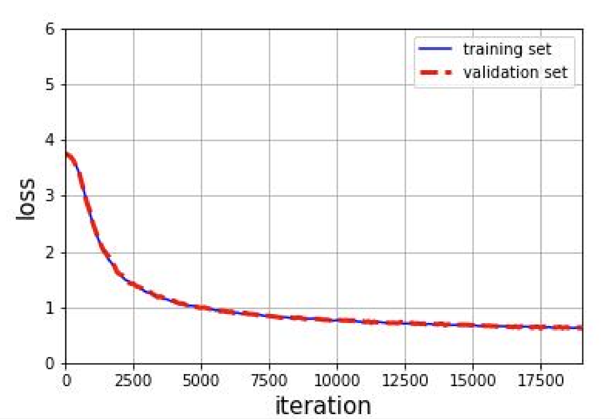
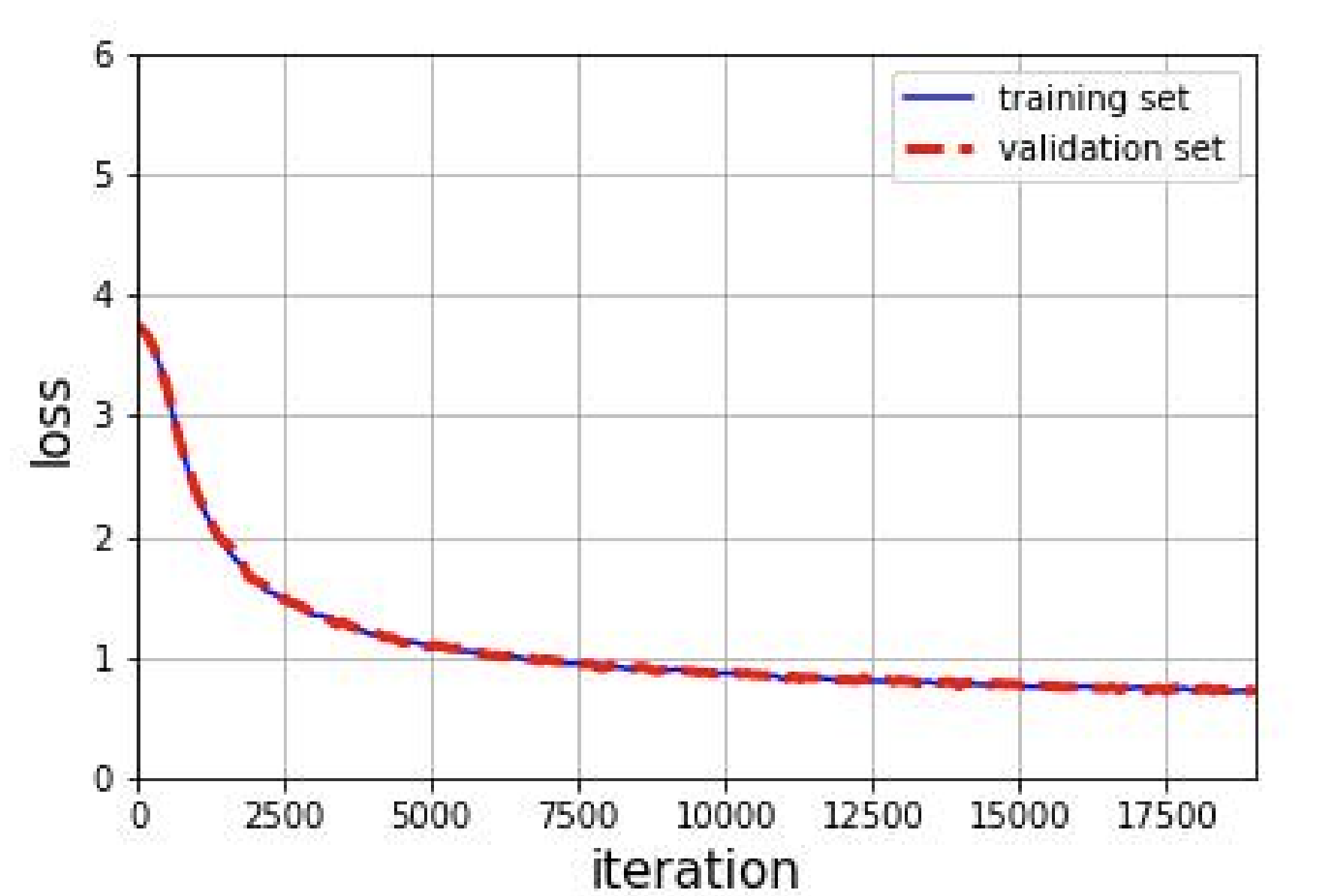
The number of replications in Algorithm 1 is set as . We apply the SA in Eq.1 with mini-batches and the batch size is set as , which takes about seconds to run in python in a desktop with Intel i7-6700 CPU @ 3.40 GHz for each iteration. Each epoch contains iterations which takes about five hours to run. The step size is set as and the noise variance is set as . Peng et al. present many training results of the GLR method on classifying the handwritten data included in the python sklearn package. In Figure.5, we show the training and validation errors of ANNs with the Sigmoid and threshold activation functions (as plotted in Figure.2) in the MNIST dataset, and the errors of ANNs converge fast after epochs ( iterations).
3.3 Robustness to Adversarial Attacks
3.3.1 Adversarial Samples
We generate the adversarial samples by an ANN with two hidden layers (as depicted in (b) of Figure.4). The ANNs are trained and validated by the BP method. The limited-memory Broyden–Fletcher–Goldfarb–Shanno (L-BFGS)(C. Szegedy & Fergus 2014) and fast gradient sign method (FGSM)(Goodfellow et al. 2014) are used to generate the adversarial samples of images randomly chosen from the testing set. The adversarial samples of the images generated by FGSM are shown in Figure.6.

3.3.2 Adversarial Test
Adversarial test is performed on several single hidden layer ANNs (Figure.4(a)) with different activation and loss functions. The accuracy is measured by the percentage of correct predictions over all adversarial samples. The ANN with the same structure in (a) of Figure.4 trained by BP is used as the baseline for comparisons. Table.1 presents the results when adversarial samples are generated by the ANN with two hidden layers (Figure.4(b)). The accuracies of the prediction on the original samples and the adversarial samples generated by the aforementioned two methods are reported.
| Activations Entropy | Orig | Adv_L_BFGS | Adv_FGSM |
| Sigmoid (trained by BP) | |||
| Sigmoid | |||
| Threshold | |||
| Activations 0-1 loss | Orig | Adv_L_BFGS | Adv_FGSM |
| Sigmoid | |||
| Threshold |
Besides the Sigmoid and threshold activation functions, three other discontinuous activation functions are also used in the experiments. Each test runs for 12 epochs and all of them demonstrate high accuracies on predicting the original samples after training. We also test the performance of an ANN with 0-1 loss function (the loss is 0 for a correct prediction and 1 otherwise), trained by the GLR. The ANN with 0-1 loss converges slower than the classic cross entropy loss (see Table.1), so we run 24 epochs in training.
In Tables.1 , an ANN with one hidden layer trained by the BP method reaches an accuracy of in predicting the original samples. However, the accuracy of the same ANN reduces dramatically to and in predicting the adversarial samples generated by L_BFGS and FGSM, respectively. This substantiates an observation in literature, i.e., the same adversarial samples can effectively attack ANNs under different architectures.
All ANNs with the cross-entropy loss function trained by the GLR method achieve accuracies in predicting original samples comparable to the ANN trained by the BP method (above in accuracy). Notice that GLR can train the ANNs with discontinuous activation functions, e.g., threshold function, and discontinuous loss functions, e.g, 0-1 loss, which cannot be handled by BP. Moreover, the ANNs trained by the GLR method have much higher accuracies (about increase) in predicting adversarial samples compared to the ANN trained by the BP method. Another interesting observation is that although the ANNs with 0-1 loss only reach accuracies less than 90% in predicting original samples, they might lead to even higher accuracies in predicting the adversarial samples than the ANNs with the cross-entropy loss.
3.4 Robustness to Natural Noises
Different from adversarial attack where the input images are affected by small, additive, classifier-tailored perturbations, natural noises add small, general, classifier-agnostic perturbations to the input images. In Hendrycks & Dietterich 2018, an IMAGENET-C benchmark generated from IMAGENET offers various corruption types with five severity levels for each type. In this work, we apply four algorithms to generate the corrupted samples for the MINST dataset. Assume the accuracy of the corruption type at the severity level for model is defined as , and then the average accuracy is defined as the evaluation metrics:
| (6) |
|
Sigmoid | Threshold |
|
| ||||||||
| Original | ||||||||||||
| Gaussian Noise | ||||||||||||
| Impulse Noise | ||||||||||||
| Glass Blur | ||||||||||||
| Contrast | ||||||||||||
| Average |
We compute the average accuracy under four types of natural noises. The images corrupted by the Gaussian noises under five levels of severity are shown in Figure 7. In Table.2, the ANN trained by the GLR method has a better performance than that trained by the BP method. Although the performance of the ANN with 0-1 loss is worse than that with a cross-entropy loss, an ANN with 0-1 loss achieves the best performance in predicting the images corrupted by the natural noises.

4 Conclusions
In this work, a GLR method is proposed for training ANNs with neuronal noises. Unlike the classic BP method, the GLR trains ANNs directly by the loss value rather than the gradient of loss and can handle ANNs with discontinuous activation and loss functions because it does not differentiate the loss output. Therefore, the GLR method could be a powerful tool to explore some brain-like learning mechanisms which allow more freedom to better represent the surrounding environment. The robustness of all ANNs trained by the GLR method is significantly improved compared with the ANN with the Sigmoid activation function and cross-entropy loss function trained by the BP method, which indicates that the new training method is a very promising tool for enhancing the security of ANNs used in practice.
A future direction lies in reducing the variance of the stochastic gradient estimation for ANNs and speed up the training procedure, so that our method can be used in the deep learning ANNs with higher complexity. Adding regularization functions to the loss function for further improving robustness also deserves future research.
References
- Asmussen & Glynn (2007) Asmussen, S. and Glynn, P. W. Stochastic Simulation: Algorithms and Analysis, volume 57. Springer Science & Business Media, 2007.
- Azulay & Weiss (2018) Azulay, A. and Weiss, Y. Why do deep convolutional networks generalize so poorly to small image transformations? CoRR, abs/1805.12177, 2018. URL http://arxiv.org/abs/1805.12177.
- Bastani et al. (2016) Bastani, O., Ioannou, Y., Lampropoulos, L., Vytiniotis, D., Nori, A., and Criminisi, A. Measuring neural net robustness with constraints. NeurIPS, 2016.
- C. Szegedy & Fergus (2014) C. Szegedy, W. Zaremba, I. S. J. B. D. E. I. G. and Fergus, R. Intriguing properties of neural networks. In International Conference on Learning Representations, 2014.
- Carlini & Wagner (2017) Carlini, N. and Wagner, D. Towards evaluating the robustness of neural networks. In Security and Privacy (SP), 2017 IEEE Symposium on, pp. 39–57, 2017.
- Dan et al. (2018) Dan, H., Mazeika, M., Wilson, D., and Gimpel, K. Using trusted data to train deep networks on labels corrupted by severe noise. NeurIPS, 2018.
- Dayan & Abbott (2018) Dayan, P. and Abbott, L. Theoretical Neuroscience. The MIT Press, 2018.
- Elsayed et al. (2018) Elsayed, G. F., Shankar, S., Cheung, B., Papernot, N., Kurakin, A., Goodfellow, I. J., and Sohl-Dickstein, J. Adversarial examples that fool both human and computer vision. CoRR, abs/1802.08195, 2018.
- Esteva et al. (2017) Esteva, A., Kuprel, B., Novoa, R. A., Ko, J., Swetter, S. M., Blau, H. M., and Thrun, S. Dermatologist-level classification of skin cancer with deep neural networks. Nature, 542:115–, 2017.
- Fu (2015) Fu, M. C. Stochastic gradient estimation. In Fu, Michael C. (ed.), Chapter 5 in Handbooks of Simulation Optimization, pp. 105–147. Springer, 2015.
- Glasserman (1991) Glasserman, P. Gradient Estimation via Perturbation Analysis. Kluwer Academic Publishers, Boston, 1991.
- Goodfellow et al. (2014) Goodfellow, I., Shlens, J., and Szegedy, C. Explaining and harnessing adversarial examples. arXiv, preprint arXiv:1412.6572, 2014.
- Graves et al. (2013) Graves, A., Mohamed, A., and Hinton, G. Speech recognition with deep recurrent neural networks. In 2013 IEEE International Conference on Acoustics, Speech and Signal Processing, pp. 6645–6649, 2013.
- Gulshan et al. (2016) Gulshan, V., Peng, L., Coram, M., Stumpe, M. C., Wu, D., Narayanaswamy, A., Venugopalan, S., Widner, K., Madams, T., Cuadros, J., Kim, R., Raman, R., Nelson, P. Q., Mega, J., and Webster, D. Development and validation of a deep learning algorithm for detection of diabetic retinopathy in retinal fundus photographs. JAMA, 2016.
- Haykin (2009) Haykin, S. S. Neural Networks and Learning Machines, volume 3. Pearson Upper Saddle River, NJ, USA:, 2009.
- He et al. (2016) He, K., Zhang, X., Ren, S., and Sun, J. Deep residual learning for image recognition. In Conference on Computer Vision and Pattern Recognition, pp. 770–778, 2016.
- Heidergott & Leahu (2010) Heidergott, B. and Leahu, H. Weak differentiability of product measures. Mathematics of Operations Research, 35(1):27–51, 2010.
- Hendrycks & Dietterich (2018) Hendrycks, D. and Dietterich, T. G. Benchmarking neural network robustness to common corruptions and perturbations. CoRR, abs/1807.01697, 2018. URL http://arxiv.org/abs/1807.01697.
- Ho & Cao (1991) Ho, Y.-C. and Cao, X.-R. Discrete Event Dynamic Systems and Perturbation Analysis. Kluwer Academic Publishers, Boston, MA, 1991.
- Hong (2009) Hong, L. J. Estimating quantile sensitivities. Operations Research, 57(1):118–130, 2009.
- Kushner & Yin (2003) Kushner, H. J. and Yin, G. G. Stochastic Approximation and Recursive Algorithms and Applications. Springer, 2003.
- (22) Peng, Y., Xiao, L., Heidergott, B., Hong, L. J., and Lam, H. Stochastic gradient estimation for artificial neural network. URL https://ssrn.com/abstract=3318847.
- Peng et al. (2018) Peng, Y., Fu, M. C., Hu, J.-Q., and Heidergott, B. A new unbiased stochastic derivative estimator for discontinuous sample performances with structural parameters. Operations Research, 66(2):487–499, 2018.
- Pflug (1996) Pflug, G. C. Optimization of Stochastic Models. Kluwer Academic, Boston, 1996.
- Recht et al. (2018) Recht, B., Roelofs, R., Schmidt, L., and Shankar, V. Do CIFAR-10 classifiers generalize to cifar-10? CoRR, abs/1806.00451, 2018. URL http://arxiv.org/abs/1806.00451.
- Rubinstein & Shapiro (1993) Rubinstein, R. Y. and Shapiro, A. Discrete Event Systems: Sensitivity Analysis and Stochastic Optimization by the Score Function Method. Wiley, New York, 1993.
- Seyed-Mohsen Moosavi-Dezfooli & Frossard (2016) Seyed-Mohsen Moosavi-Dezfooli, A. F. and Frossard, P. Deepfool: a simple and accurate method to fool deep neural networks. In Proceedings of the IEEE Conference on Computer Vision and Pattern Recognition, pp. 2574–2582, 2016.
- Silver et al. (2016) Silver, D., Huang, A., Maddison, C. J., Guez, A., Sifre, L., Driessche, G. V. D., Schrittwieser, J., Antonoglou, I., Panneershelvam, V., and Lanctot, M. Mastering the game of go with deep neural networks and tree search. Nature, 529(7587):484–489, 2016.