Laser-Driven Electron Lensing in Silicon MicrostructuresPreprint: APS/123-QED
Abstract
We demonstrate a laser-driven, tunable electron lens fabricated in monolithic silicon. The lens consists of an array of silicon pillars pumped symmetrically by two 300 fs, 1.95 m wavelength, nJ-class laser pulses from an optical parametric amplifier. The optical near-field of the pillar structure focuses electrons in the plane perpendicular to the pillar axes. With 100 10 MV/m incident laser fields, the lens focal length is measured to be 50 4 m, which corresponds to an equivalent quadrupole focusing gradient of 1.4 0.1 MT/m. By varying the incident laser field strength, the lens can be tuned from a 21 2 m focal length ( MT/m) to focal lengths on the cm-scale.
pacs
41.75.Jv,41.75.FrThe Dielectric Laser Accelerator (DLA) is a dielectric microstructure which harnesses the large electric fields in femtosecond-pulsed lasers to produce an electron linear accelerator with acceleration gradients orders of magnitude higher than conventional metal accelerators England et al. 2014; Wootton et al. 2017. The microstructure is a sub-wavelength grating whose optical near-field is phasematched to a propagating electron beam, thereby accelerating the electron beam. The accelerator size is commensurate with its drive wavelength; while advantageous in some respects, this presents new challenges. To confine an electron beam to a m-scale DLA channel, a lens with focusing strength many orders of magnitude higher than currently available is necessary.
In conventional accelerators, the magnetic quadrupole is the preferred lens for charged particle focusing due to its high focusing strength, low dispersion, and linear field gradient Smith 1970. Focusing strength is defined as , where is the focal length and the length of the lens. The magnetic quadrupole focusing strength is Rossbach and Schmüser 1993. It is common to compare lens strengths by their equivalent quadrupole field gradient , and this convention is adopted throughout this letter. The required for DLA is between 100-1000 kT/m, set by the resonant defocusing forces of the synchronous accelerating mode England et al. 2014; Ody et al. 2017; Niedermayer et al. 2018. Conventional quadrupoles can achieve a of only 500 T/m Strait; Eichner et al. 2007; Becker et al. 2009. The other commonly employed static-field lenses, einzel lenses H Read et al. 2001 and solenoids Kumar 2009, are also far too weak to achieve effective confinement. To realize an electron linac on-chip, a new type of lens, as proposed in Niedermayer et al. 2018, must be designed.

The ideal lens for DLA beam confinement would be stable, high-power, tunable, and monolithically integrable into the current architecture. Monolithic integration is especially critical, as alignment tolerances for m-scale beamlines are measured in nanometers, and such tight alignment tolerances are only realistically accessible by use of a monolithic fabrication procedure for both lens and accelerator.
Electrodynamic lenses can provide the required focusing strength. Active plasma lenses have focusing gradients exceeding 3 kT/m van Tilborg et al. 2015, while plasma wakefield lensing has focusing strengths on the order of 1 MT/m Ng et al. 2001; Chiadroni et al. 2018. Plasma wakefield lensing fits naturally with plasma-based accelerators Kuschel et al. 2016, and provides more than sufficient focusing strength. However, integration of plasma lenses with photonic accelerators would require generation of stable plasmas on-chip that are compatible with the accelerator nanofabrication processes.
Strong lensing effects can also be derived from the optical near-fields of femtosecond-pulsed lasers. Recently, a laser-driven lens with a 190 m focal length was demonstrated by McNeur et al. McNeur et al. 2018, which is estimated to have an equivalent of 85 kT/m. The evanescent fields near a curved silicon grating generate a focusing field in the plane of the wafer. However, in single gratings there are always undesirable out-of-plane deflection forces Leedle et al. 2015. Moreover, the curvature of the grating causes undesirable coupling of the two transverse planes, which complicates the lens implementation in a multi-stage accelerator design.
In this letter, we demonstrate a laser-driven, solid-state electron lens based on the DLA architecture, which was first proposed by Plettner et al. in Plettner et al. 2009; Plettner et al. 2011, and whose specific architecture is discussed by Leedle et al. in Leedle et al. 2018. When illuminated by two laser pulses, each with an electric field of 100 10 MV/m, its focal length is measured to be 50 4 m ( MT/m). The lens strength is continuously tunable, and we demonstrate its tuning to a focal length below 21 2 m ( MT/m). The lensing behavior agrees well with simulation, and we provide a linearized model that approximates the lens focal length. This lens architecture adds no additional complexity to the accelerator fabrication process, as it uses identical procedures and can be integrated directly into the lithographic mask. The demonstrated focusing strength is sufficient to confine an electron beam to a m-scale beamline. We propose that this lens be used in an Alternating Phase Focusing (APF) scheme Niedermayer et al. 2018, which allows stable beam confinement and acceleration over arbitrary distances.
The lens structure (Fig. 1) is fabricated from monolithic 510 -cm B:Si, and consists of 2 rows of 15 pillars, with periodicity nm and a 375 nm wide channel between the rows. The pillars are elliptical (613 nm x 459 nm), with a height of 2.7 m. The electron beam passes though the central channel, where it interacts with two 300 25 fs laser pulses with a center wavelength of 1.950 0.005 m and a 1/ radius of 20 2 m. Following the lens is 39.6 m of drift space, then an aperture consisting of two 4 m x 4 m x 2.7 m silicon blocks with a gap of 150 10 nm between them.
The electromagnetic fields in the lens are described following Leedle et al. 2018; Niedermayer et al. 2017a; Wei et al. 2017. We consider a dual-pillar structure semi-infinite in , symmetric in , and periodic in . The device is illuminated by two counter-propagating -polarized plane waves, incident from the directions (Fig. 1), each with electric field . The electrons travel in with velocity . The synchronicity (or phasematching) condition between the laser field and the electron is
| (1) |
where is the central laser wavelength and is the structure periodicity. The Lorentz force on an electron inside the structure, assuming Eq. 1 is satisfied and non-phasematched harmonics are negligible, is
| (2) |
where , is the wavevector of the evanescent field, is the elementary charge, and is the magnitude of the synchronous accelerating field at Niedermayer et al. 2017a. We assume a laser phase such that is purely real and positive, and define the structure constant . is the phase of the electron relative to the optical cycle of the plane wave, and is the relative phase between the counter-propagating waves. The force along the coordinate is zero by the semi-infinite assumption. Previous experimental results, as well as 3-D FDTD simulations, indicate that the semi-infinite approximation works well for 2.7 m tall (or taller) pillars Leedle et al. 2018. The magnitude of the transverse and longitudinal forces differ by a factor of , as expected from the Panofsky-Wenzel theorem K. H. Panofsky and A. Wenzel 1956.
For in-phase drive lasers ( = 0) and assuming perfect synchronicity, the focal length of a device with periods is approximately
| (3) |
Eq. S5 is valid for a sufficiently small such that the thin-lens approximation holds. The lens strengths considered here restrict the validity of Eq. S5 to devices with .
Neglecting phase slippage due to acceleration, valid for short structures, the energy gain in the = 0 mode is
| (4) |
For out-of-phase drive lasers (), there exists, to first order in , a constant deflection force whose direction varies sinusoidally with . Further discussion of the accelerator modes is contained in the Supplementary Material.
The electron bunch is modeled as a collection of normally distributed , , and values. Each electron experiences a focal length drawn from the distribution of Eq. S5, and for an electron beam much longer than an optical cycle (6 fs), the electrons within the bunch stochastically sample all possible focal lengths. To measure the minimum lens focal length, a very small aperture is placed one focal length from the lens and acts as a temporal filter, biasing electron detection towards the focusing phases () over the defocusing phases ().
The electron beam used in this experiment was produced with a 300 25 fs FWHM, 100 kHz, 256 nm laser pulse incident on a flat copper cathode. The electron beam has a circular gaussian spatial profile and a 4 width of 780 63 nm at the lens entrance, measured by a knife edge scan. The geometric 1-D emittance is estimated to be 0.5 nm rad. The beam energy is 89.4 0.1 keV, which corresponds to . The beam current is set to 730 200 /s to avoid energy broadening from space charge effects at the cathode. Each electron pulse at the interaction point is 740 110 fs FWHM in length, measured by cross correlation with a 300 25 fs laser pulse.

43 8% of electrons are transmitted through the aperture with the laser (and thus the lens) off. Leakage through the silicon blocks is small; the blocks block 95% of incident electrons. For the focusing mode, an increase in electron transmission through the aperture is expected, with maximal transmission when the drift length is matched to the lens focal length. “Contrast,” the percent increase in electron transmission when the lens is turned on (Eq. 5), quantifies this increase.
| (5) |
is the electron transmission with the lens on, and is the electron transmission with the lens off. After the aperture, the electrons travel through a magnetic spectrometer with an energy resolution of 100 eV, and are detected on a microchannel plate detector.
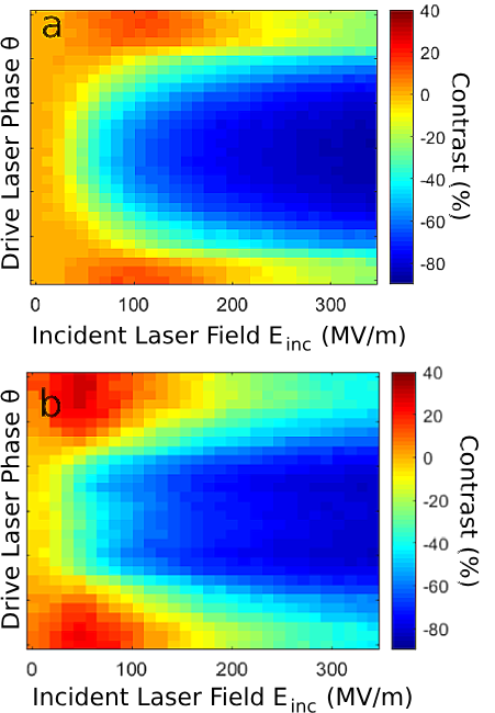
Electron transmission simulations were carried out for a range of incident laser fields () and drive laser phases () (Fig. 2a). Due to the long bunch length, the increased transmission from the focusing phases is partially offset by the decreased transmission from the defocusing phases. Thus, the expected contrast in this operating mode is low, only 11%. However, for the mode, a large transmission decrease for all values of is expected.

In Fig. 2b, the parameter space simulated in Fig. 2a is measured. The experimental data agrees qualitatively with the simulation. There is a small contrast peak at 100 10 MV/m for , with a large region of strong negative contrast in the region.
The energy modulation and contrast as a function of drive laser phase is shown in Fig. 3. The sinusoidal variation of energy gain and contrast predicted by Eq. 4 is demonstrated, and the peak transmission and peak energy modulation occur at the same , in agreement with theory.
Fig. 4 plots contrast in the focusing mode as a function of , to aid a visual comparison between simulation and experiment. The co-location of the peak contrast for simulation and experiment is apparent. Duplicate runs omitted from Fig. 2b for visual clarity are included in Fig. 4.
The contrast peak at 100 10 MV/m ( 38 MV/m) corresponds to a focal length of 64 6 m in the linearized approximation (Eq. S5). Our experimentally measured focal length, defined as the total distance from the lens principal plane to aperture center, is measured to be 50 4 m ( MT/m). The measured focal power is greater than predicted by Eq. S5, indicating that the thin-lens approximation breaks down at these lens strengths. The simulation, which uses the forces from Eq. 2, accurately predicts the incident field which gives peak contrast. Because the measured focal length will always be less than that predicted by the linearized approximation, Eq. S5 can be considered a lower bound on the lens focusing strength. The incident laser field is increased to a maximum of 306 16 MV/m, corresponding to a linearized focal length of 21 2 m ( MT/m).

The structure constant was measured to be 0.38 0.04 for this structure, with a maximum acceleration gradient of 111 6 MeV/m. Previous work with similar structures has demonstrated , with MeV/m Leedle et al. 2018.
The main experimental limitation was electron beam pointing instability. The electron beam could be stably aligned to the aperture for approximately 60 s, limited by thermal drifts. An averaging time of 3 s per data point (2000 electrons) was chosen to compromise between high frequency and low frequency noise. The effects of random beam motion are partially compensated by normalizing the total number of transmitted electrons to the fraction of electrons detected at the initial beam energy of 89.4 keV. Since the laser pulse is shorter than the electron pulse, many electrons within the pulse do not interact with the laser, and these electrons are all detected at 89.4 keV. The fluctuation of the electron counts detected at 89.4 keV serves as an instantaneous measure of electron beam misalignment. The details are included in the Supplementary Material.
The focusing strength scales as , which is a less favorable scaling than the scaling of solenoids or the scaling of quadrupoles. The equivalence point is found by equating of a quadrupole lens to of a DLA lens and solving for . The equivalence point here is 35 MeV. This can be increased by increasing either the electric field or the lens length. Efficient laser-electron interaction requires that the lens material refractive index be greater than Hughes et al. 2018; Kozák et al. 2017. Silicon has at 2.0 m, corresponding to a lower limit of (23 keV).
The lens focal length is continuously variable from approximately 20 microns to the cm-scale. However, electron pulses of duration are required for use as a single focal length lens. Fortunately, a pulse train created using the same DLA architecture Niedermayer et al. 2018; Niedermayer et al. 2017b has the correct microbunch length and periodicity. The use of evanescent fields to focus electrons necessitates a narrow aperture, and so its emittance acceptance is small. The beam emittance in this lens is not conserved, however the emittance growth due to field nonlinearity is quite small. Achievable spot sizes are limited by third-order aberrations from the sinh focusing profile. Lens nonlinearities are treated more fully by Niedermayer et al. in Niedermayer et al. 2017a; Niedermayer et al. 2018.
We propose to use this lens in an Alternating Phase Focusing (APF) confinement scheme. Briefly, lens stages are alternated with drift sections chosen to provide a specific phase offset between lens stages. For example, a drift length of one half-period is equivalent to a phase delay in , which reverses the sign of the lens focal length. If the phase offsets are chosen appropriately, it is possible to achieve stable confinement in both the transverse and longitudinal directions simultaneously, which can then be combined with high gradient acceleration, as detailed in Niedermayer et al. 2018. The confinement requirements for DLA are set by the resonant defocusing forces England et al. 2014; Ody et al. 2017; Niedermayer et al. 2018, and since the defocusing forces are exactly those forces described by Eq. 2, the lensing forces presented here have precisely the same strength as the resonant defocusing itself. Thus, using this architecture, the focusing strength requirement for confinement in DLA is satisfied automatically, even for the large defocusing forces present in high-gradient accelerators Cesar et al. 2018.
In summary, we have demonstrated a laser-driven, continuously tunable electrodynamic lens with a focusing strength equivalent to those observed in plasmas Ng et al. 2001; Chiadroni et al. 2018 and which far exceeds any static-field lens. Its design is easily and monolithically integrable with current photonic accelerator architectures, and its strength is sufficient to confine an electron beam to an accelerator channel less than 1 m wide for an arbitrary distance Niedermayer et al. 2018. This removes a major roadblock in the development of scalable on-chip electron accelerators.
References
- England et al. (2014) R. Joel England, Robert J. Noble, Karl Bane, David H. Dowell, Cho Kuen Ng, James E. Spencer, Sami Tantawi, Ziran Wu, Robert L. Byer, Edgar Peralta, Ken Soong, Chia Ming Chang, Behnam Montazeri, Stephen J. Wolf, Benjamin Cowan, Jay Dawson, Wei Gai, Peter Hommelhoff, Yen Chieh Huang, Chunguang Jing, Christopher McGuinness, Robert B. Palmer, Brian Naranjo, James Rosenzweig, Gil Travish, Amit Mizrahi, Levi Schachter, Christopher Sears, Gregory R. Werner, and Rodney B. Yoder. Dielectric laser accelerators. Reviews of Modern Physics, 86(4):1337–1389, dec 2014. ISSN 15390756. doi:10.1103/RevModPhys.86.1337. URL https://link.aps.org/doi/10.1103/RevModPhys.86.1337.
- Wootton et al. (2017) K P Wootton, R J England, Sami Tantawi, Slac National, Menlo Park, R W Aßmann, Ingmar Hartl, F X Kärtner, Willi Kuropka, Frank Mayet, A Ruehl, Deutsches Elektronen-synchrotron, D Hamburg, Leonid Rivkin, École Polytechnique, Fédérale De Lausanne, Ch Lausanne, Peter Hommelhoff, Johannes Illmer, Ang Li, J Mcneur, Anna Mittelbach, Norbert Schönenberger, Alex Tafel, Friedrich-alexander Universität Erlangen-nürnberg, Rasmus Ischebeck, Paul Scherrer Institut, Ch-Villigen Psi, Y Lee, Minghao Qi, West Lafayette, D S Black, R L Byer, Huiyang Deng, Shanhui Fan, J S Harris, Tyler Hughes, Neil Sapra, Olav Solgaard, J Vučković, B M Cowan, Tech-x Corporation, Thilo Egenolf, Uwe Niedermayer, Technische Universität Darmstadt, Max-planck-institut Quantenoptik, and D Garching. Towards a Fully Integrated Accelerator on a Chip : Dielectric Laser Acceleration ( DLA ) From the Source To Relativistic Electrons. Proceedings of IPAC, 4744:2520–2525, 2017. doi:10.3204/PUBDB-2017-05953. URL http://inspirehep.net/record/1608652/.
- Smith (1970) D. L. Smith. Focusing properties of electric and magnetic quadrupole lenses. Nuclear Instruments and Methods, 79(1):144–164, mar 1970. ISSN 0029554X. doi:10.1016/0029-554X(70)90020-0. URL https://www.sciencedirect.com/science/article/pii/0029554X70900200.
- Rossbach and Schmüser (1993) J Rossbach and P Schmüser. Basic course on accelerator optics, 1993. URL http://inspirehep.net/record/347558/files/Cern.pdfhttp://cds.cern.ch/record/247501.
- Ody et al. (2017) A. Ody, P. Musumeci, J. Maxson, D. Cesar, R.J. England, and K.P. Wootton. Flat electron beam sources for DLA accelerators. Nuclear Instruments and Methods in Physics Research Section A: Accelerators, Spectrometers, Detectors and Associated Equipment, 865:75–83, sep 2017. ISSN 01689002. doi:10.1016/j.nima.2016.10.041. URL https://linkinghub.elsevier.com/retrieve/pii/S0168900216310877.
- Niedermayer et al. (2018) Uwe Niedermayer, Thilo Egenolf, Oliver Boine-Frankenheim, and Peter Hommelhoff. Alternating-Phase Focusing for Dielectric-Laser Acceleration. Phys. Rev. Lett., 121(21):214801, nov 2018. doi:10.1103/PhysRevLett.121.214801. URL https://link.aps.org/doi/10.1103/PhysRevLett.121.214801.
- (7) J. Strait. Very high gradient quadrupoles. In PACS2001. Proceedings of the 2001 Particle Accelerator Conference (Cat. No.01CH37268), volume 1, pages 176–180. IEEE. ISBN 0-7803-7191-7. doi:10.1109/PAC.2001.987463. URL http://ieeexplore.ieee.org/document/987463/.
- Eichner et al. (2007) T Eichner, Florian Grüner, S Becker, Matthias Fuchs, D Habs, R Weingartner, U Schramm, H Backe, Peter Kunz, and Werner Lauth. Miniature magnetic devices for laser-based, table-top free-electron lasers. Physical Review Special Topics-accelerators and Beams - PHYS REV SPEC TOP-AC, 10, 2007. doi:10.1103/PhysRevSTAB.10.082401.
- Becker et al. (2009) S. Becker, M. Bussmann, S. Raith, M. Fuchs, R. Weingartner, P. Kunz, W. Lauth, U. Schramm, M. El Ghazaly, F. Grüner, H. Backe, and D. Habs. Characterization and tuning of ultrahigh gradient permanent magnet quadrupoles. Physical Review Special Topics - Accelerators and Beams, 12(10):102801, 2009. ISSN 1098-4402. doi:10.1103/PhysRevSTAB.12.102801. URL https://link.aps.org/doi/10.1103/PhysRevSTAB.12.102801.
- H Read et al. (2001) F H Read, A Adams, and J R Soto-Montiel. Electrostatic cylinder lenses. I. Two element lenses. Journal of Physics E: Scientific Instruments, 4:625, 2001. doi:10.1088/0022-3735/4/9/001.
- Kumar (2009) V Kumar. Understanding the focusing of charged particle beams in a solenoid magnetic field. American Journal of Physics, 77:737–741, aug 2009. doi:10.1119/1.3129242.
- van Tilborg et al. (2015) J van Tilborg, Sven Steinke, C G R Geddes, Nicholas Matlis, Brian Shaw, Anthony Gonsalves, J V Huijts, Kei Nakamura, Joost Daniels, C B Schroeder, Carlo Benedetti, E Esarey, S S Bulanov, Nadezhda Bobrova, P Sasorov, and Wim Leemans. Active Plasma Lensing for Relativistic Laser-Plasma-Accelerated Electron Beams. Physical Review Letters, 115:184802, 2015. doi:10.1103/PhysRevLett.115.184802.
- Ng et al. (2001) J. S. T. Ng, P. Chen, H. Baldis, P. Bolton, D. Cline, W. Craddock, C. Crawford, F. J. Decker, C. Field, Y. Fukui, V. Kumar, R. Iverson, F. King, R. E. Kirby, K. Nakajima, R. Noble, A. Ogata, P. Raimondi, D. Walz, and A. W. Weidemann. Observation of plasma focusing of a 28.5 gev positron beam. Phys. Rev. Lett., 87:244801, Nov 2001. doi:10.1103/PhysRevLett.87.244801. URL https://link.aps.org/doi/10.1103/PhysRevLett.87.244801.
- Chiadroni et al. (2018) Enrica Chiadroni, Maria Pia Anania, M Bellaveglia, Angelo Biagioni, Fabrizio Bisesto, E Brentegani, Fabio Cardelli, Alessandro Cianchi, G Costa, D Giovenale, Giampiero Di Pirro, Massimo Ferrario, Francesco Filippi, Gallo Alessandro, Anna Giribono, Alberto Marocchino, Andrea Mostacci, Luca Piersanti, Riccardo Pompili, and Arie Zigler. Overview of plasma lens experiments and recent results at SPARC_LAB. Nuclear Instruments and Methods in Physics Research Section A: Accelerators, Spectrometers, Detectors and Associated Equipment, 2018. doi:10.1016/j.nima.2018.02.014.
- Kuschel et al. (2016) S Kuschel, D Hollatz, T Heinemann, O Karger, M B Schwab, D Ullmann, A Knetsch, A Seidel, C Rödel, M Yeung, M Leier, A Blinne, H Ding, T Kurz, D J Corvan, A Sävert, S Karsch, M C Kaluza, B Hidding, and M Zepf. Demonstration of passive plasma lensing of a laser wakefield accelerated electron bunch. Phys. Rev. Accel. Beams, 19(7):71301, jul 2016. doi:10.1103/PhysRevAccelBeams.19.071301. URL https://link.aps.org/doi/10.1103/PhysRevAccelBeams.19.071301.
- McNeur et al. (2018) Joshua McNeur, Martin Kozák, Norbert Schönenberger, Kenneth J Leedle, Huiyang Deng, Andrew Ceballos, Heinar Hoogland, Axel Ruehl, Ingmar Hartl, Ronald Holzwarth, Olav Solgaard, James S Harris, Robert L Byer, and Peter Hommelhoff. Elements of a dielectric laser accelerator. Optica, 5(6):687–690, jun 2018. doi:10.1364/OPTICA.5.000687. URL http://www.osapublishing.org/optica/abstract.cfm?URI=optica-5-6-687.
- Leedle et al. (2015) Kenneth J Leedle, R Fabian Pease, Robert L Byer, and James S Harris. Laser acceleration and deflection of 96.3 keV electrons with a silicon dielectric structure. Optica, 2(2):158–161, feb 2015. doi:10.1364/OPTICA.2.000158. URL http://www.osapublishing.org/optica/abstract.cfm?URI=optica-2-2-158.
- Plettner et al. (2009) T Plettner, R L Byer, C. McGuinness, and P Hommelhoff. Photonic-based laser driven electron beam deflection and focusing structures. Physical Review Special Topics - Accelerators and Beams, 12(10):101302, 2009. ISSN 1098-4402. doi:10.1103/PhysRevSTAB.12.101302. URL https://journals.aps.org/prab/pdf/10.1103/PhysRevSTAB.12.101302https://link.aps.org/doi/10.1103/PhysRevSTAB.12.101302.
- Plettner et al. (2011) T. Plettner, R L Byer, and B. Montazeri. Electromagnetic forces in the vacuum region of laser-driven layered grating structures. Journal of Modern Optics, 58(17):1518–1528, oct 2011. ISSN 09500340. doi:10.1080/09500340.2011.611914. URL http://www.tandfonline.com/doi/pdf/10.1080/09500340.2011.611914?needAccess=truehttp://www.tandfonline.com/doi/abs/10.1080/09500340.2011.611914.
- Leedle et al. (2018) Kenneth J. Leedle, Dylan S. Black, Yu Miao, Karel E. Urbanek, Andrew Ceballos, Huiyang Deng, James S. Harris, Olav Solgaard, and Robert L. Byer. Phase-dependent laser acceleration of electrons with symmetrically driven silicon dual pillar gratings. Optics Letters, 43(9):2181, may 2018. ISSN 0146-9592. doi:10.1364/OL.43.002181. URL https://www.osapublishing.org/abstract.cfm?URI=ol-43-9-2181.
- Niedermayer et al. (2017a) Uwe Niedermayer, Thilo Egenolf, and Oliver Boine-Frankenheim. Beam dynamics analysis of dielectric laser acceleration using a fast 6D tracking scheme. Physical Review Accelerators and Beams, 20(11):111302, nov 2017a. ISSN 24699888. doi:10.1103/PhysRevAccelBeams.20.111302. URL https://link.aps.org/doi/10.1103/PhysRevAccelBeams.20.111302https://arxiv.org/pdf/1707.09815.pdfhttp://arxiv.org/abs/1707.09815.
- Wei et al. (2017) Y Wei, M Ibison, G Xia, J D A Smith, and C P Welsch. Dual-grating dielectric accelerators driven by a pulse-front-tilted laser. Appl. Opt., 56(29):8201–8206, oct 2017. doi:10.1364/AO.56.008201. URL http://ao.osa.org/abstract.cfm?URI=ao-56-29-8201.
- K. H. Panofsky and A. Wenzel (1956) W K. H. Panofsky and W A. Wenzel. Some Considerations Concerning the Transverse Deflection of Charged Particles in Radio‐Frequency Fields. Review of Scientific Instruments, 27, 1956. doi:10.1063/1.1715427.
- Hughes et al. (2018) Tyler W. Hughes, Si Tan, Zhexin Zhao, Neil V. Sapra, Kenneth J. Leedle, Huiyang Deng, Yu Miao, Dylan S. Black, Olav Solgaard, James S. Harris, Jelena Vuckovic, Robert L. Byer, Shanhui Fan, R. Joel England, Yun Jo Lee, and Minghao Qi. On-Chip Laser-Power Delivery System for Dielectric Laser Accelerators. Physical Review Applied, 9(5):054017, may 2018. ISSN 23317019. doi:10.1103/PhysRevApplied.9.054017. URL https://link.aps.org/doi/10.1103/PhysRevApplied.9.054017.
- Kozák et al. (2017) M Kozák, P Beck, H Deng, J McNeur, N Schönenberger, C Gaida, F Stutzki, M Gebhardt, J Limpert, A Ruehl, I Hartl, O Solgaard, J S Harris, R L Byer, and P Hommelhoff. Acceleration of sub-relativistic electrons with an evanescent optical wave at a planar interface. Opt. Express, 25(16):19195–19204, aug 2017. doi:10.1364/OE.25.019195. URL http://www.opticsexpress.org/abstract.cfm?URI=oe-25-16-19195.
- Niedermayer et al. (2017b) Uwe Niedermayer, Oliver Boine-Frankenheim, and Thilo Egenolf. Designing a Dielectric Laser Accelerator on a Chip. Journal of Physics: Conference Series, 874(1):12041, 2017b. URL http://stacks.iop.org/1742-6596/874/i=1/a=012041.
- Cesar et al. (2018) D Cesar, S Custodio, J Maxson, P Musumeci, X Shen, E Threlkeld, R J England, A Hanuka, I V Makasyuk, E A Peralta, K P Wootton, and Z Wu. High-field nonlinear optical response and phase control in a dielectric laser accelerator. Communications Physics, 1(1), 2018. doi:10.1038/s42005-018-0047-y.
Supplementary Material
I Summary
Supplementary material for Laser-Driven Electron Lensing in Silicon Microstructures, by Black et al. This appendix contains derivations of some equations stated in the main paper, as well as the details of the normalization scheme used to process the reported experimental data. All references refer to the bibliography in the main paper.
II DLA Lens Focal Length
For convenience, the definitions of various parameters are restated here.
As in the main manuscript, we consider a dual-pillar structure semi-infinite in , symmetric in , and periodic in (following [20-22]). The device is illuminated by two counter-propagating -polarized plane waves, incident from the direction. The electrons travel along with velocity , is the laser center wavelength, is the structure periodicity, , is the wavevector of the evanescent field, is the elementary charge, is the magnitude of the synchronous accelerating field at , is the phase of the electron relative to the laser optical cycle of the plane wave within the periodic structure, and is the relative phase between the counter-propagating waves. We assume a laser phase such that is purely real and positive.
Beginning from the Lorentz force (Eq. 2 in the main paper), the transverse force seen by an electron at a given can be written as a superposition of a cosh term and a sinh term, which correspond to the deflecting and focusing modes, respectively.
| (S1) |
The relative drive laser phase controls the behavior of the device. For in-phase drive lasers ( = 0) and assuming perfect synchronicity, integrating in time across one period (see [21]) gives
| (S2) |
Applying and expanding to first order in yields
| (S3) |
The angular deviation of the electron trajectory over one DLA period near the center of the channel is
| (S4) |
For a sufficiently small number of periods such that is nearly constant, the total angular deflection is . In analogy with the first order approximation of lens focal length, , the focal length of the DLA lens is approximately,
| (S5) |
Eq. S5 is valid only for cases where the focal length is much less than the length of the lens. For a lens of periods, the lens length is and the thin lens approximation holds when
| (S6) |
For the lens strengths considered here, the lens can be considered “thin” if . Longer lenses must be modeled as thick lenses (see [6]).
III Energy Gain of Short DLA Structures
On-axis (), the electron sees a longitudinal force of
| (S7) |
Since energy gain is small for small , phase slippage due to acceleration can be neglected, and the total energy gain over periods is found by integrating over the length of the structure, yielding an on-axis energy gain of
| (S8) |
IV Deflection Forces
For , the forces in the transverse direction are given by
| (S9) |
In the limit of small deviations from the axis, is
| (S10) |
For a lens with a channel width much less than , higher order terms may be neglected and the deflection force is approximately constant in magnitude across the lens channel. The direction of the deflection force varies sinusoidally with , and the magnitude is directly proportional to the laser field strength via . Operated in this mode, the structure can be used as an optical frequency streaking element.
The angular deflection for a single period is easily calculated by integration of over one period, yielding, to leading order,
| (S11) |
Since the deflection force is constant to leading order in , angular deflection for periods is well approximated by
| (S12) |
The same caveats that limit the applicability of the thin-lens approximation in the previous sections also apply here, with the additional constraint that a beam deflected uniformly by each period of accelerator structure will hit the channel wall after some distance, limiting the maximum angular deflection produced by this structure.
V Peak Normalization
V.1 Introduction
The electron beam misalignment caused by slow thermal drifts is the main source of experimental noise. A common technique for removing external effects from a measured signal is to compare the experiment to a simultaneous reference experiment. In light optics, for example, a beamsplitter can be used to create a reference beam against which the experiment may be compared.
An identical reference electron beam cannot be created for this experiment. However, since the laser pulse used to modulate the energy of the electron pulse is shorter than the electron pulse itself, there are many electrons detected which do not interact with the laser at all. The fluctuation of the non-interacting electron counts is not dependent on the laser fields, and can therefore be used as an instantaneous reference for beam alignment to the lens channel.
The non-interacting electrons are all detected at the initial beam energy (see Fig. 1). Thus, by filtering the detected electrons with a magnetic spectrometer and normalizing the total electron counts to the electron counts at the initial beam energy, it is possible to partially separate the electron count fluctuations due to the laser fields from the fluctuations due to beam misalignment. In other words, the height of the central energy peak (Fig. 1) constitutes an instantaneous pseudo- reference beam against which total electron transmission can be compared. Not all of the electrons which appear at the central energy peak are non-interacting. But, since the electron pulse used in this experiment is nearly twice as long as the laser pulse, the majority of the electrons detected at the initial beam energy are, in fact, non-interacting.
V.2 A Note on the Experimental Procedure
The independent variables in the experiment are the peak electric field of one drive laser , and the relative phase between the two drive lasers . The dependent variable is the electron counts measured on the detector. Each data point taken in the experiment was taken as part of a “phase sweep,” which consists of holding constant while is varied linearly, and continuously measuring the electron energy spectrum as a function of phase (see Fig. 4 in the main paper or Fig. 3 in the Supplementary Material for an example of a phase sweep). During the phase sweep, individual data points are collected, consisting of an electron energy spectrum with an averaging time of 3 s (2000 electrons). After each phase sweep is completed, the laser is turned off, and the energy spectrum is again measured. Then, is increased by a fixed amount, and another phase sweep is taken. In this way, the entire parameter space is sampled for both laser-on and laser-off conditions.

V.3 Notation
Let the total number of electron counts (“transmission”) measured at an energy for some be denoted by . In order to reduce visual clutter, this quantity will be written simply as when the functional dependence is not relevant. This experiment depends on measuring the “contrast” between a laser-on condition and a laser-off condition. These two conditions will be specified by a superscript when it is necessary to distinguish them, e.g. (the transmission with the laser on) or (the transmission with the laser off), but the superscript will be omitted when the equation can be applied equally to both laser conditions, i.e. an equation involving is valid for both and . The superscript will also be used to explicitly denote quantities which are measured or simulated when it is necessary to distinguish the two, e.g. is the simulated transmission for the laser-on condition.
Normalized quantities in the simplified scheme will be written with a hat, e.g. . Corrected, normalized quantities will be written with a tilde, e.g. .
V.4 Simplified Normalization Scheme
Define the normalization factor as
| (S13) |
where is the central beam energy, and is the average over all drive laser phases for a single phase sweep. is then a function of and , defined for each data point, whose mean over a single phase sweep is 1, and whose fluctuations are directly proportional to the electron counts detected with energy .
Define the total electron transmission as
| (S14) |
and the normalized transmission as
| (S15) |
Contrast is defined as
| (S16) |
The normalized contrast is then
| (S17) |
V.5 Corrected Normalization Scheme
The simplified normalization scheme above warps the parameter space (see Fig. 2), preventing a legitimate comparison of simulated and measured data. The normalization scheme must be corrected such that the parameter space in the zero-noise case remains invariant under normalization.
To construct the corrected normalized transmission , the normalization factor is simulated for the entire parameter space, and an inverse normalization is applied to both the simulated and the measured data, i.e. for simulated data,
| (S18) |
and for measured data,
| (S19) |
Clearly, for simulated data, the corrected, normalized transmission is identical to the actual electron transmission . For measured data, this is not necessarily true. In the following section, the desired signal, the “true” transmission , which is assumed to be identical to the simulated value, will be explicitly separated from any undesirable random fluctuations in the real experiment, denoted by . Define
| (S20) |
The measured normalization factor is
| (S21) |
The mean value of the drift over time is uncorrelated with drive laser phase . Assuming that averages to zero over many periods of , it can be neglected in the denominator, giving
| (S22) |
Again, to reduce visual clutter, the transmission ratios will be defined as
| (S23) |
The measured, normalized transmission ratio is, explicitly
| (S24) |

Applying the simulated correction factor according to Eq. S13 gives the corrected, normalized transmission ratio
| (S25) |
Which can be rewritten in terms of the “true” transmission ratio as
| (S26) |
where each quantity is understood to be evaluated for the same , . If any noise present in the measurement is a constant fraction of the signal over the whole electron energy spectrum, i.e. , then, even for cases where , and the expression for the corrected, normalized contrast reduces to the true contrast,
| (S27) |
An example phase sweep in unprocessed form and the correction of both slow drift and higher frequency fluctuations with the corrected peak normalization scheme is shown in Fig. 3. As Fig. 3 clearly shows, the corrected normalization scheme is effective in removing electron count fluctuations due to drift while preserving the general shape of the curve.
The maximum energy modulation for a given is robust to beam misalignment. Because the maximum energy modulation occurs at the edge of the lens channel, where the evanescent field is strongest, the maximum energy modulation for a given does not change with small misalignments of the electron beam - so long as the beam remains partially within the channel, some electrons from the beam experience the largest possible energy modulation provided by the optical mode. In this regime, the maximum energy modulation depends solely on the amplitude and phase of the drive lasers, whose fluctuations are small compared to the electron count fluctuations introduced by beam pointing instability.
Shown below each panel in Fig. 3 is the electron energy spectrum as a function of frame number (time) as the laser phase is linearly increased. The correlation between the contrast and the energy broadening is supported by analytical considerations (See Eq. 4 in the main paper), and is clearly seen in Fig. 3. This provides a good sanity check for our normalization scheme.
Restating the key result, if the noise is evenly distributed in electron energy space, then the corrected, normalized contrast is equal to the true contrast , and the correct (de-noised) value of contrast for each data point can be recovered through the peak normalization scheme without use of a distinct reference beam.