Optimal Contract Design for Incentive-Based Demand Response

Refer to the timeline shown in Figure 1. The true base load (without any manipulation) is given by $l$. At time $t_{1}$, the customer calculates the effort $a$ she is willing to put in for achieving the load reduction $x$ during the DR event. The load reduction is according to the probability density function $f(x|a)$ which is public knowledge. We assume that an effort $a$ costs the customer $h(a)$ ($h(a)$ is convex and $h(0)=0$). Further, this effort and the planned load reduction $(a,x)$ depends on private knowledge at the customer and hence can be calculated by the customer, but not by the DRA. For instance, a factory might be able to induce a large load reduction with a small effort based on its assembly line requirements given the orders it has to fulfill. After this calculation, the customer at time $t_{1}$ may increase (or decrease) the load by an amount $i$ in anticipation of the DR event.

At time $t_{2}$, the DR event begins and the DRA calls on the customer to decrease her load. The customer now makes the effort $a$ yielding a reduction of the load by $x$. The DR event ends at $t_{3}$ with the customer having decreased the load by an amount $R(x)$ (which is often simplified to $R$). Note that the planned reduction in the load is $x=R(x)-i(x)$, while the false reported load reduction is $R(x)$. We also show the times $t_{0}$, $t_{4}$ and $t_{5}$ in the timeline in Figure 1. At time $t_{0}$ (much before $t_{1}$), the contract is signed between the DRA and the customer, while at times $t_{4}$ and $t_{5}$, the customer is paid by the DRA according to the contract we will propose in the sequel. We note that $t_{0}$ is sufficiently early, so that at $t_{0}$, the customer does not know the local conditions and must consider her expected utility according to the probability density function $f(x|a)$.

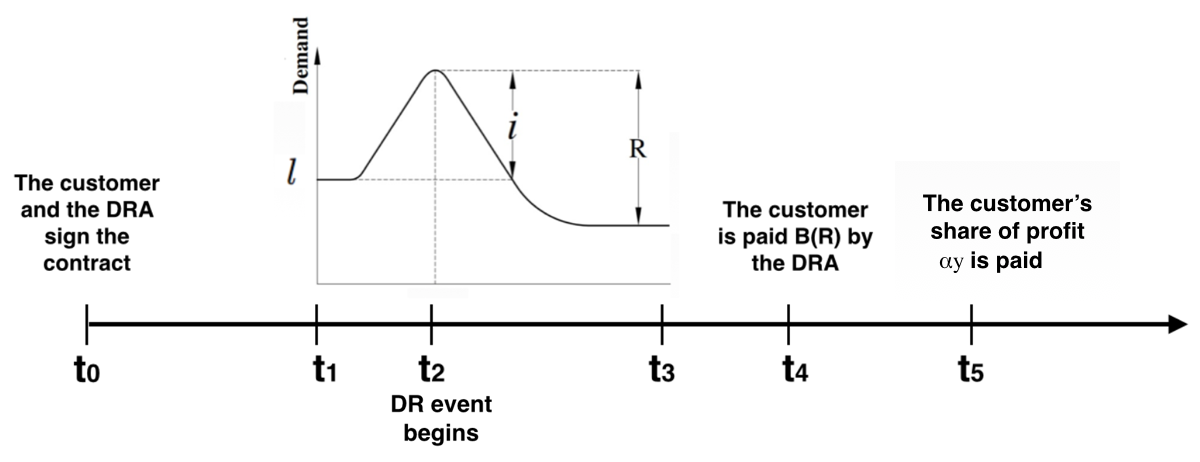
The time $t_{4}$ is sufficiently close to the DR event, so that, the realized value of $x$ is not known at time $t_{4}$ to the DRA. The customer needs to be paid at least in part at $t_{4}$ to incentivize her to participate in the DR event. However, at some (much) later time $t_{5}$, the DRA may be able to estimate the realized value of $x$, possibly with some error. This noisy estimate can be obtained by, e.g., large scale data analysis on all similar customers on that day or historical behavioral of the same customer. We denote this estimate by $y$ where $y=x+n$. We assume that the random variables $X$ and $N$ are independent and $N\sim\mathcal{N}(m_{n},\sigma_{n}^{2})$.

We model the falsification cost incurred by the customer (e.g. extra charge paid for boosting her consumption) by a quadratic function for simplicity and denote this cost as $g(R-x)=\frac{(R-x)^{2}}{2}$.

The problem is for the DRA to design a contract that maximizes his own profit. Since this profit depends on the load reduction by the customer, the contract must induce a rational customer to choose an action $a$ and a report $R$ that are optimal for the DRA. The profit for the DRA occurs due to the load reduction by the customer, modulo any payments made to the customer as part of her contract. We discuss the intuition for the proposed contract through some examples.

Next, we propose a contract structure free from the shortcomings of these intuitive contracts.

Inspired by managerial contracts studied e.g. in [9, 10], we propose a contract of the form $(\alpha,B(R))$ in which $\alpha$ refers to the share of his own profit that the DRA provides to the customer, while $B(R)$ refers to the payment made in proportion to the reported reduction $R(x)$. Referring to Figure 1, to incentivize the customers to participate in the program, $B(R)$ is paid at $t_{4}$. However, the shares (even though they are allotted at $t_{0}$) can be encashed only at a much later time $t_{5}$ when an estimated value of the profit can be calculated and revealed. Note that the portion of the payment corresponding to the share $\alpha$ is calculated on the basis of the noisy estimate $y$ of $x$. Thus, the customer’s utility is given by

while the DRA utility is given by

It is worth pointing out that the customer will report a load reduction to realize $x$; therefore, $R$ is a function of $x$, not $y$.

Thus, the optimization problem to be solved by DRA (subject to participation and rationality constraints for customer) is given by

We now describe the constraints for the optimization problem in (3).

1. 1.

   Rationality in the choice of effort: The first assumption is that the customer chooses the level of effort $a$ to maximize her expected utility $\E[V]$. Thus, the first two constraints are given by $\frac{\partial\E[V]}{\partial a}=0$ and $\frac{\partial^{2}\E[V]}{\partial a^{2}}\leq 0$ where the expectation is taken with respect to $x$ and $y$.

2. 2.

   Ex ante individual rationality: The expected utility of the customer must be positive to ensure that she participates in the DR event. This implies a constraint of the form $\E[V]\geq 0$.

3. 3.

   Interim individual rationality: We impose that the customer must be incentivized to continue even though she can choose to leave after she makes effort $a$ and sees her comfort reduced. We impose this constraint as

   $$W\stackrel{{\scriptstyle\triangle}}{{=}}V+h(a)\geq 0.$$

   (4)

4. 4.

   Incentive compatibility: We impose two further constraints $R^{\prime}(x)\geq 0$ and $W_{x}=\alpha+g^{\prime}(R(x)-x))$ as incentive compatibility constraints that ensure truthtelling by the customer in the conditional direct revelation contract [9].

Thus, the optimization problem can be rewritten as

subject to:

We will present the optimal contract in Section III. The solution depends on the properties of the pdfs $f_{X|A}(x|a)$ that describes the planned reduction $x$ based on effort $a$ of the customer and $f_{N}(n)$ which is the pdf of the estimation error in the knowledge of $x$ in the long term. We make the following assumptions about these functions :

1. 1.

   Assumption $\mathcal{A}_{1}$: The cdf $F_{X|A}(x|a)$ of $f_{X|A}(x|a)$ is strictly decreasing, convex and continuously differentiable in $a$ for all $x$ and for all $a$. This is a natural assumption implying that higher customer effort induces a first-order stochastic improvement in the distribution of load reduction and results in diminishing marginal returns from effort.

2. 2.

   Assumption $\mathcal{A}_{2}$: $f_{X|A}(x|a)>0$ for all $x$ and $a$. Further, there exists $M>0$ such that for all $x$ and $a,$ $f_{X|A}(x|a)<M$ and $\frac{\partial{f_{X|A}(x|a)}}{\partial{x}}<M$.

3. 3.

   Assumption $\mathcal{A}_{3}$: $\frac{\partial{f_{X|A}(x|a)}}{\partial{x}}\geq 0$ for all $a>0$. This assumption implies that positive values of load reduction are more likely than zero values of load reduction.

4. 4.

   Assumption $\mathcal{A}_{4}$: $(F_{X|A}(x|a)-1)/f_{X|A}(x|a)$ is strictly concave in $x$ for all $a$ and $F_{a}(x|a)/f_{X|A}(x|a)$ is strictly convex in $x$ for all $a$ where

   $$F_{a}(x|a)=\frac{\partial{F_{X|A}(x|a)}}{\partial{a}}.$$

   (7)

   Assumption $\mathcal{A}_{4}$ is provided for the proof of corollary 3 (in section IV) where we restrict to Gaussian distribution for $x$ and $n$ for simplicity.

We can obtain a clearer interpretation of over-reporting (inflation of base load) and underreporting (reduction of base load) through the following result that specifies the form of the reporting function.

In order to study the optimal compensation, we first present the following result without proof.

We notice that the bonus can be considered to be a function of the savings $x$ and written as $B(x)$. Further, the bonus is related to $W$ as

In order to compare the optimal reporting as a function of the noise in the estimation of the profit made due to the reduction of load, we need to investigate the optimal reporting function for the cases when $x$ is realized at $t_{5}$ exactly and with some error. Equation (16) shows the relation between the optimal reporting function and the true profit with estimation error. In the absence of any error, the expression reduces to

For simplicity, we assume for the next result that $f_{Y|A}(y|a)=\mathcal{N}(m(a),{\sigma_{y}}^{2})$ and $f_{N}(n)=\mathcal{N}(0,\sigma_{n}^{2}).$ It is worth pointing out that assumptions $\mathcal{A}_{1}-\mathcal{A}_{4}$ hold in this case (for Gaussian distribution). By definition, $x=y-n$ will be a Gaussian random variable and $f_{X|A}(x|a)=\mathcal{N}(m(a),{\sigma_{x}}^{2})$. Notice when there is no error $x=y$ and $f_{X|A}(z|a)=f_{Y|A}(z|a)=\mathcal{N}(m(a),{\sigma_{y}}^{2})$, in the case of noise; however, $x=y-n$ so $f_{X|A}(z|a)=\mathcal{N}(m(a),{\sigma_{x}}^{2}={\sigma_{y}}^{2}-\sigma_{n}^{2})$. Accordingly, suppose $f_{Y|A}(z|a)$ and $f_{X|A}(z|a)$ represent the pdf of $x$ in the absence and presence of noise. Comparing $f_{X|A}(z|a)$ and $f_{Y|A}(z|a)$ for a variable $0\leq z\leq 1$, we obtain:

where $c=m(a)+\sigma_{x}\sigma_{y}\sqrt{\frac{2\ln(\frac{\sigma_{x}}{\sigma_{y}})}{\sigma_{x}^{2}-\sigma_{y}^{2}}}$.

The following result shows that the optimal contract must utilize the option of giving shares to the customer.

References

- [1] J. S. Vardakas, N. Zorba, and C. V. Verikoukis, “A survey on demand response programs in smart grids: Pricing methods and optimization algorithms,” Communications Surveys & Tutorials, IEEE, vol. 17, no. 1, pp. 152–178, 2015.
- [2] R. Deng, Z. Yang, M.-Y. Chow, and J. Chen, “A survey on demand response in smart grids: Mathematical models and approaches,” Industrial Informatics, IEEE Transactions on, vol. 11, no. 3, pp. 570–582, 2015.
- [3] M. H. Albadi and E. El-Saadany, “Demand response in electricity markets: An overview,” in IEEE power engineering society general meeting, vol. 2007, 2007, pp. 1–5.
- [4] F. A. Qureshi, T. T. Gorecki, and C. Jones, “Model predictive control for market-based demand response participation,” in 19th World Congress of the International Federation of Automatic Control, no. EPFL-CONF-197950, 2014.
- [5] A.-H. Mohsenian-Rad, V. W. Wong, J. Jatskevich, and R. Schober, “Optimal and autonomous incentive-based energy consumption scheduling algorithm for smart grid,” in Innovative Smart Grid Technologies (ISGT), 2010. IEEE, 2010, pp. 1–6.
- [6] P. Samadi, A.-H. Mohsenian-Rad, R. Schober, V. W. Wong, and J. Jatskevich, “Optimal real-time pricing algorithm based on utility maximization for smart grid,” in Smart Grid Communications (SmartGridComm), 2010 First IEEE International Conference on. IEEE, 2010, pp. 415–420.
- [7] A. J. Roscoe and G. Ault, “Supporting high penetrations of renewable generation via implementation of real-time electricity pricing and demand response,” IET Renewable Power Generation, vol. 4, no. 4, pp. 369–382, 2010.
- [8] Q. Wang, M. Liu, and R. Jain, “Dynamic pricing of power in smart-grid networks,” in Decision and Control (CDC), 2012 IEEE 51st Annual Conference on. IEEE, 2012, pp. 1099–1104.
- [9] K. J. Crocker and T. Gresik, “Optimal compensation with earnings manipulation: Managerial ownership and retention,” mimeo, Tech. Rep., 2010.
- [10] K. J. Crocker and J. Slemrod, “The economics of earnings manipulation and managerial compensation,” The RAND Journal of Economics, vol. 38, no. 3, pp. 698–713, 2007.
- [11] A. Seierstad and K. Sydsaeter, Optimal control theory with economic applications. Elsevier North-Holland, Inc., 1986.
- [12] G. Maggi and A. Rodriguez-Clare, “On countervailing incentives,” Journal of Economic Theory, vol. 66, no. 1, pp. 238–263, 1995.
- [13] E. Nekouei, T. Alpcan, and D. Chattopadhyay, “Game-theoretic frameworks for demand response in electricity markets,” Smart Grid, IEEE Transactions on, vol. 6, no. 2, pp. 748–758, 2015.
- [14] A.-H. Mohsenian-Rad, V. W. Wong, J. Jatskevich, R. Schober, and A. Leon-Garcia, “Autonomous demand-side management based on game-theoretic energy consumption scheduling for the future smart grid,” Smart Grid, IEEE Transactions on, vol. 1, no. 3, pp. 320–331, 2010.