![[Uncaptioned image]](1902.00134v2/cern.jpg) CERN-LPCC-2018-04
August 11, 2026
CERN-LPCC-2018-04
August 11, 2026
Higgs Physics at the HL-LHC and HE-LHC Report from Working Group 2 on the Physics of the HL-LHC, and Perspectives at the HE-LHC
The discovery of the Higgs boson in 2012, by the ATLAS and CMS experiments, was a success achieved with only a percent of the entire dataset foreseen for the LHC. It opened a landscape of possibilities in the study of Higgs boson properties, Electroweak Symmetry breaking and the Standard Model in general, as well as new avenues in probing new physics beyond the Standard Model. Six years after the discovery, with a conspicuously larger dataset collected during LHC Run 2 at a 13 \UTeVcentre-of-mass energy, the theory and experimental particle physics communities have started a meticulous exploration of the potential for precision measurements of its properties. This includes studies of Higgs boson production and decays processes, the search for rare decays and production modes, high energy observables, and searches for an extended electroweak symmetry breaking sector. This report summarises the potential reach and opportunities in Higgs physics during the High Luminosity phase of the LHC, with an expected dataset of pp collisions at 14 \UTeV, corresponding to an integrated luminosity of 3 ab-1. These studies are performed in light of the most recent analyses from LHC collaborations and the latest theoretical developments. The potential of an LHC upgrade, colliding protons at a centre-of-mass energy of 27 \UTeVand producing a dataset corresponding to an integrated luminosity of 15 ab-1, is also discussed.
1 Introduction
One of the main goals of the physics program at the Large Hadron Collider is to elucidate the origin of electroweak symmetry breaking.
Relativistic quantum field and gauge theories have been remarkably successful to describe fundamental particles and their interactions. In this context, the seminal work of Brout, Englert [1], Higgs [2, 3, 4] and Guralnik, Hagen and Kibble [5, 6], has provided a consistent mechanism for the generation of gauge boson masses. The Glashow-Weinberg-Salam theory extended this mechanism proposing a theory of the electroweak interactions [7, 8, 9], introducing a doublet of complex scalar fields, which couples also to fermions, providing them with a mass which would otherwise be absent. This is now known as the Standard Model (SM) of particle physics. A complete and detailed description of the Higgs mechanism can be found at [10]. A salient prediction of the theory is the presence of a Higgs boson. The discovery of the Higgs boson with a mass of 125 \UGeV, during the first run of the LHC at reduced centre-of-mass energies of 7 \UTeVand 8 \UTeV, is a landmark result that has reshaped the landscape of High Energy physics [11, 12]. The mass of the Higgs boson is particularly favourable as it allows to measure directly a large number of its couplings. It has also important consequences in terms of probing the self-consistency of the Standard Model both through the global fit of precision observables and through its interpretation as a measure of the Higgs boson self coupling, allowing to extrapolate the SM at higher energies and verify the stability of the vacuum.
The existence of the Higgs boson as a light scalar leads to the hierarchy or naturalness problem, as its mass at the weak scale happens to be particularly sensitive to general larger scales beyond the SM (BSM), therefore apparently requiring a large fine tuning of fundamental parameters. Addressing the naturalness problem is and has been for decades one of the main guiding principles for the development of theories beyond the Standard Model. There are two main classes of theories attempting to address the naturalness problem: the first are weakly coupled theories, where the Higgs boson remains an elementary scalar and its mass is protected by additional symmetries, as in Supersymmetric theories. The second are strongly coupled solutions, which involve new strong interactions at approximately the \UTeVscale and deliver naturally light composite scalars as Pseudo Nambu-Goldstone bosons. Both approaches can have large effects on the phenomenology of the Higgs particle and in some cases predict new states that could be observed at the LHC.
Other questions of fundamental importance can affect the phenomenology of the Higgs boson. The question of the nature of the Electroweak Phase transition is strongly intertwined with Higgs physics where, in many scenarios, a detailed study of the Higgs pair production can reveal the strength of the transition. Similarly, certain models of Dark Matter involve potentially large effects on the phenomenology of the Higgs particle. These fundamental questions, and many more, can be addressed by the study of the Higgs boson at the LHC and its high luminosity (HL) and high energy (HE) upgrades.
Since the discovery, a large campaign of measurements of the properties of the Higgs boson has started, including exclusive production modes and differential cross sections. Many new ideas have emerged during the completion of this program. This chapter presents a reappraised estimate of the potential of the HL-LHC and the HE-LHC projects to measure the properties of the Higgs boson, highlighting the opportunities for measurements of fundamental importance.
Section 2 presents the foreseen program for precision measurements of the Higgs boson coupling properties through exclusive production modes and differential cross sections. Section 3 presents the potential to measure double Higgs production and to constrain the Higgs trilinear coupling, both through the double Higgs production and indirect probes from single Higgs boson production. Section 4 is devoted to a new class of measurements unique to the HL-HE program: high-energy probes. These include Higgs processes like associated production of a Higgs and a or boson, or vector boson fusion (VBF), for which the centre-of-mass energy is not limited to the Higgs mass, and it extends to Drell Yan, di-boson processes and vector boson scattering, which provide a context in which high-energy measurements can be associated with precision observables. Section 5 focuses on measurements of the Higgs mass and opportunities for the measurement of the Higgs boson width. Section 6 describes the constraints on the invisible decays of the Higgs boson and the indirect constraints on the couplings of the Higgs boson to undetected particles from the measurement of the Higgs boson couplings, in particular in the framework of Higgs portal and dark matter models. Section 7 will discuss approaches to constrain light and non diagonal Higgs Yukawa couplings directly and indirectly. Section 8 is devoted to a global interpretation of the measurements in the framework of the Standard Model Effective Field Theory. Section 9 is devoted to the discussion of the prospects for probing additional Higgs bosons both with a mass above or below 125 \UGeV, and for discovering a wide range of exotic Higgs boson decays.
1.1 Experimental analysis methods and objects definitions
Different approaches have been used by the experiments and in theoretical prospect studies, hereafter named projections, to assess the sensitivity in searching for new physics at the HL-LHC and HE-LHC. For some of the projections, a mix of the approaches described below is used, in order to deliver the most realistic result. The total integrated luminosity for the HL-LHC dataset is assumed to be fb-1 at a centre-of-mass energy of \UTeV. For HE-LHC studies the dataset is assumed to be ab-1 at a centre-of-mass of \UTeV. The effect of systematic uncertainties is taken into account based on the studies performed for the existing analyses and using common guidelines for projecting the expected improvements that are foreseen thanks to the large dataset and upgraded detectors, as described in Section 1.1.3.
Detailed-simulations are used to assess the performance of reconstructed objects in the upgraded detectors and HL-LHC conditions, as described in Sections 1.1.1,1.1.2. For some of the projections, such simulations are directly interfaced to different event generators, parton showering (PS) and hadronisation generators. Monte Carlo (MC) generated events are used for SM and BSM processes, and are employed in the various projections to estimate the expected contributions of each process.
Extrapolations of existing results rely on the existent statistical frameworks to estimate the expected sensitivity for the HL-LHC dataset. The increased centre-of-mass energy and the performance of the upgraded detectors are taken into account for most of the extrapolations using scale factors on the individual processes contributing to the signal regions. Such scale factors are derived from the expected cross sections and from detailed simulation studies.
Fast-simulations are employed for some of the projections in order to produce a large number of Monte Carlo events and estimate their reconstruction efficiency for the upgraded detectors. The upgraded CMS detector performance is taken into account encoding the expected performance of the upgraded detector in Delphes [13], including the effects of pile-up interactions. Theoretical contributions use Delphes with the commonly accepted HL-LHC card corresponding to the upgraded ATLAS and CMS detectors.
Parametric-simulations are used for some of the projections to allow a full re-optimisation of the analysis selections that profit from the larger available datasets. Particle-level definitions are used for electrons, photons, muons, taus, jets and missing transverse momentum. These are constructed from stable particles of the MC event record with a lifetime larger than s within the observable pseudorapidity range. Jets are reconstructed using the anti- algorithm [14] implemented in the FastJet [fastjet] library, with a radius parameter of 0.4. All stable final-state particles are used to reconstruct the jets, except the neutrinos, leptons and photons associated to or boson or lepton decays. The effects of an upgraded ATLAS detector are taken into account by applying energy smearing, efficiencies and fake rates to generator level quantities, following parametrisations based on detector performance studies with the detailed simulations. The effect of the high pileup at the HL-LHC is incorporated by overlaying pileup jets onto the hard-scatter events. Jets from pileup are randomly selected as jets to be considered for analysis with efficiency, based on studies of pile-up jet rejection and current experience.
1.1.1 ATLAS and CMS performance
The expected performance of the upgraded ATLAS and CMS detectors has been studied in detail in the context of the Technical Design Reports and subsequent studies; the assumptions used for this report and a more detailed description are available in Ref. [16, 17]. For CMS, the object performance in the central region assumes a barrel calorimeter ageing corresponding to an integrated luminosity of fb-1.
The triggering system for both experiments will be replaced and its impact on the triggering abilities of each experiment assessed; new capabilities will be added, and, despite the more challenging conditions, most of the trigger thresholds for common objects are expected to either remain similar to the current ones or to even decrease [ATLAS_TDAQ_TDR, CMSL1interim].
The inner detector is expected to be completely replaced by both experiments, notably extending its coverage to . The performance for reconstructing charged particles has been studied in detail in Ref. [ATLAS_Pixel_TDR, ATLAS_Strip_TDR, CMS_Tracker_TDR].
Electrons and photons are reconstructed from energy deposits in the electromagnetic calorimeter and information from the inner tracker[23, CMS_Barrel_TDR, Collaboration:2293646, 26]. Several identification working points have been studied and are employed by the projection studies as most appropriate.
Muons are reconstructed combining muon spectrometer and inner tracker information [27, CMS_Muon_TDR].
Jets are reconstructed by clustering energy deposits in the electromagnetic and hadronic calorimeters[29, 23, CMS_Barrel_TDR] using the anti- algorithm[14]. B-jets are identified via -tagging algorithms. B-tagging is performed if the jet is within the tracker acceptance (). Multivariate techniques are employed in order to identify jets and jets, and were fully re-optimised for the upgraded detectors [ATLAS_Pixel_TDR, CMS_Tracker_TDR]. An 70% jet efficiency working point is used, unless otherwise noted.
High boosted jets are reconstructed using large-radius anti- jets with a distance parameter of 0.8. Various jet substructure variables are employed to identify boosted W/Z/Higgs boson and top quark jets with good discrimination against generic QCD jets.
Missing transverse energy is reconstructed following similar algorithms as employed in the current data taking. Its performance has been evaluated for standard processes, such as top pair production [ATLAS_Pixel_TDR, Contardo:2020886].
1.1.2 LHCb
The LHCb upgrades are shifted with respect to those of ATLAS and CMS. A first upgrade will happen at the end of Run 2 of the LHC, to run at a luminosity five times larger () in LHC Run 3 compared to those in Runs 1 and 2, while maintaining or improving the current detector performance. This first upgrade phase (named Upgrade I) will be followed by by the so-called Upgrade II phase (planned at the end of Run 4) to run at an even more challenging luminosity of .
The LHCb MC simulation used in this document mainly relies on the Pythia 8 generator [32] with a specific LHCb configuration [33], using the CTEQ6 leading-order set of parton density functions [34]. The interaction of the generated particles with the detector, and its response, are implemented using the Geant toolkit [35, 36], as described in Ref. [37].
The reconstruction of jets is done using a particle flow algorithm, with the output of this clustered using the anti-kT algorithm as implemented in FastJet, with a distance parameter of 0.5. Requirements are placed on the candidate jet in order to reduce the background formed by particles which are either incorrectly reconstructed or produced in additional pp interactions in the same event.
Concerning the increased pile-up, different assumptions are made, but in general the effect is assumed to be similar to the one in Run 2.
1.1.3 Treatment of systematic uncertainties
It is a significant challenge to predict the expected systematic uncertainties of physics results at the end of HL-LHC running. It is reasonable to anticipate improvements to techniques of determining systematic uncertainties over an additional decade of data-taking. To estimate the expected performance, experts in the various physics objects and detector systems from ATLAS and CMS have looked at current limitations to systematic uncertainties in detail to determine which contributions are limited by statistics and where there are more fundamental limitations. Predictions were made taking into account the increased integrated luminosity and expected potential gains in technique. These recommendations were then harmonised between the experiments to take advantage of a wider array of expert opinions and to allow the experiments to make sensitivity predictions on equal footing [16, 17]. For theorists’ contributions, a simplified approach is often adopted, loosely inspired by the improvements predicted by experiments.
General guide-lining principles were defined in assessing the expected systematic uncertainties. Theoretical uncertainties are assumed to be reduced by a factor of two with respect to the current knowledge, thanks to both higher-order calculation as well as reduced parton distribution functions (PDF) uncertainties [38]. All the uncertainties related to the limited number of simulated events are neglected, under the assumption that sufficiently large simulation samples will be available by the time the HL-LHC becomes operational. For all scenarios, the intrinsic statistical uncertainty in the measurement is reduced by a factor , where L is the projection integrated luminosity divided by that of the reference Run 2 analysis. Systematics driven by intrinsic detector limitations are left unchanged, or revised according to detailed simulation studies of the upgraded detector. Uncertainties on methods are kept at the same value as in the latest public results available, assuming that the harsher HL-LHC conditions will be compensated by method improvements.
The uncertainty in the integrated luminosity of the data sample is expected to be reduced down to 1% by a better understanding of the calibration methods and their stability employed in its determination, and making use of the new capabilities of the upgraded detectors.
In addition to the above scenario (often referred to as “YR18 systematics uncertainties” scenario), results are often compared to the case where the current level of understanding of systematic uncertainties is assumed (“Run 2 systematic uncertainties”) or to the case of statistical-only uncertainties.
1.2 Implications for beyond the Standard Model theories
1.2.1 Heavy new physics: precision tests and effective field theories
Precision measurements provide an important tool to search for heavy BSM dynamics, associated with mass scales beyond the LHC direct energy reach, exploiting the fact that such dynamics can still have an impact on processes at smaller energy, via virtual effects. In this context the well-established framework of effective field theories (EFTs) allows to systematically parametrise BSM effects and how they modify SM processes. Assuming lepton and baryon number conservation, the leading such effects can be captured by dimension-6 operators,
| (1) |
for dimensionless coefficients and, for simplicity, a common suppression scale . Table 1 proposes a set of operators considered in this report. This set is redundant, in the sense that different combinations of operators might lead to the same physical effect; moreover this set is not complete, in the sense that there are more operators at dimension-6 level. In practical applications we will always be interested in identifying minimal (non-redundant) subsets of operators that contribute to a given process; we will also be interested that these operators be complete, at least under some well motivated assumption. For instance, the assumption that new physics only couples to the SM bosons, leads to the universal set of operators, from the second panel in table 1. Alternatively, the minimal flavour violation assumption [DAmbrosio:2002vsn] provides a well-motivated framework to focus on operators with a certain, family-universal, flavour structure; operators with a richer flavour structure will be studied in a dedicated section 7.
| Higgs-Only Operators | ||
| Universal Operators | ||
| and , , , , , | ||
| Non-Universal Operators that modify couplings to fermions | ||
| CP-odd operators | ||
Reduction to a minimal basis is achieved via integration by parts and field re-definitions, equivalent in practice to removing combinations proportional to the equations of motion. These imply relations between the operators of table 1; the most important ones being ( denotes here hyper-charge)
| (2) | |||
| (3) | |||
| (4) |
and similar expressions for and in terms of the products of and SM currents. Eqs. (2-4) can be used to define minimal, non-redundant operator bases; for instance, in the context of Higgs physics, the operators are retained at the expense of , , , , in what is known as the SILH basis [40], while in the opposite case we refer to the Warsaw basis [41].11 1 In addition, the SILH basis gives preference to the operators and , which are more easily found in universal BSM theories, while the Warsaw basis swaps them in terms of four-fermions operators.
These operators induce two types of effects: some that are proportional to the SM amplitudes and some that produce genuinely new amplitudes. The former are better accessed by high-luminosity experiments in kinematic regions where the SM is the largest. The most interesting example of this class for the LHC are Higgs couplings measurements in single-Higgs processes. The operators in the top panel of table 1 have the form , with denoting operators in the SM Lagrangian, and imply small modifications of the Higgs couplings to other SM fields, with respect to the SM value. These are often parametrised as rescalings of the SM rates, ( the Higgs partial width into channel ) assuming the same Lorentz structure as that of the SM, i.e. providing an overall energy-independent factor. This is known as the kappa framework [42]. We discuss Higgs couplings in detail in sections 2 and 4 .
Among effects associated with new amplitudes, that cannot be put in correspondence with the s, particularly interesting are BSM energy-growing effects. At dimension-6 level we find effects that grow at most quadratically with the energy. This implies a quadratic enhancement of the sensitivity to these effects, as we consider bins at higher and higher energy. This can be contrasted with high-intensity effects, whose sensitivity increases only with the square root of the integrated luminosity, and eventually saturates as systematics become comparable. High-energy effects are the ideal target of the HL and HE LHC programs, as we discuss in section 4. In section 8, we combine the results from the various EFT analyses and provide a global perspective on the HL and HE LHC sensitivity to EFT effects.
Ultimately, the goal of these global fits is to provide a model-independent framework to which large classes of specific models can be matched an analysed. We provide some example in section 8.
1.2.2 Light new physics: rare processes and new degrees of freedom
A complementary way to unveil BSM physics affecting the Higgs sector of Nature is the search for very rare processes involving the 125 \UGeVHiggs boson and for extended Higgs sectors.
The SM predicts several processes involving the Higgs boson to be very rare. Notable examples are the di-Higgs production, as well as the Higgs decays to first and second generation quarks and leptons. The search for these rare processes can unveil the presence of new degrees of freedom. Particularly, measurements of the di-Higgs production cross section (Sec. 3) will give constraints on the Higgs trilinear interaction, therefore providing information on electroweak symmetry breaking and allowing to set constraints on e.g. the nature of the phase transition between the trivial Higgs vacuum and the vacuum we observe at present (Sec. 3.6.2) and on the presence of extended Higgs sectors. The HL and HE stages of the LHC will be crucial to achieve this goal thanks to the relatively sizeable di-Higgs samples that will be produced: at HL-LHC and at HE-LHC (compared to the di-Higgs produced at Run 1 and 2 LHC). Furthermore, the branching ratios of SM rare Higgs decay modes such as , , and have been only mildly upper bounded by present LHC searches due in part to the low statistics (, ) and, in part, to the background limited analyses (). An important progress on these rare decay modes is expected at the HL and HE-LHC. For example, the HL-LHC will be able to discover and have a accuracy measurement of the di-muon decay mode (Sec. 2.3.8). Knowing the Higgs couplings to light quark and lepton generations will shed light on BSM flavor models and possibly on the SM flavor puzzle (Sec. 7).
Beyond rare SM Higgs processes, BSM models that contain new light degrees of freedom, , generically predict rare exotic Higgs, decays or where is a SM particle (Secs. 6 and 9.1. For a review see e.g. [43]). A typical example is the Higgs decaying to light dark matter particles. Thanks to the tiny Higgs width ( \UMeV), even very feebly coupled new light particles can lead to relatively sizeable Higgs branching ratios that can be probed by the LHC in the future. On the one hand, the HL and HE-LHC will produce huge samples of Higgs bosons from its main production mode, gluon fusion ( and , respectively). This can allow the search for super rare and low background signatures. On the other hand, the sample of Higgs bosons produced from sub-leading production modes in association with other SM particles (e.g. ) will be sizeable, increasing the discovery prospects for rare and more background limited Higgs decay signatures. Therefore, the HL/HE-LHC Higgs exotic decay program can be uniquely sensitive to the existence of a broad range of new light weakly coupled particles (on condition that trigger and analysis thresholds will be kept relatively low, to allow capturing this set of soft signatures).
In many BSM theories, electroweak symmetry is broken not only by one Higgs boson, but by several degrees of freedom. Examples are supersymmetric theories, composite Higgs theories, as well as theories of neutral naturalness. Overall, extended Higgs sectors can lead to new interesting signatures that are not contained in the SM. The search for additional Higgs bosons is a high priority for current and future colliders. The ATLAS and CMS collaborations have performed several searches for heavy neutral and charged Higgs bosons during the first two runs of the LHC. At the same time, the LHCb collaboration (as well as ATLAS and CMS) has pursued several searches for new Higgs bosons with a mass below 125 \UGeV. The reach of all these searches will expand considerably in the future and, especially, at the HL and HE-LHC. In Secs. 9.2-9.4 and 9.8 of this report, we study the prospects for testing some of the most promising signatures. Most of the BSM models that predict the existence of an extended Higgs sector, also predict a 125 \UGeVHiggs with the interactions which are generically different from the SM predictions. As we will show in Secs. 9.5-9.7, the study of the interplay between new Higgs searches and Higgs coupling measurements will be a powerful tool to probe vast regions of parameter space of BSM theories with an extended electroweak symmetry breaking sector.
2 Higgs boson precision measurements22 2 Contact Editors: S. Alioli, M. Dührssen, P. Milenovic
2.1 Introduction
The large number of events expected in almost all Higgs boson measurement channels for the HL-LHC and HE-LHC will allow very precise measurements of the Higgs boson production cross sections and its couplings to gauge bosons and fermions. In many measurement channels, the expected overall statistical, experimental and theoretical uncertainties will be comparable in size. Therefore, a close interaction between the communities of the experimental and theoretical particle physicists will be needed in order to reach the best possible measurements of the Higgs boson properties.
Experimental sensitivity for the Higgs boson properties measurements is estimated by extrapolating the performance of the existing measurements to the HL-LHC data set, assuming the experiments will have a similar level of detector and triggering performance. Results are presented for two assumptions on the size of the experimental and theoretical systematic uncertainties that will be achievable by the time of HL-LHC (so called conservative and optimistic scenarios). Details on the extrapolation methodology and scenarios will be presented in Section 2.3.
Section 2.2 provides an overview of theoretical predictions for the Higgs boson production at 14 and 27 \UTeV and of the uncertainties that are expected to be reached by the time of the final HL-LHC and HE-LHC measurements. These predictions are used as input to sensitivity studies of the ATLAS and CMS Higgs boson cross section and coupling measurements in individual channels that are summarised in Section 2.3 and for the expectations for differential cross section measurements presented in Section 2.4. Section 2.5 puts emphasis on all measurements related to the top Yukawa coupling, as this is the largest Yukawa coupling in the Standard Model with a value close to unity and, hence, of special interest in understanding the Higgs mechanism and its relation to fermions. The combination of the expected measurements in ATLAS and CMS are presented in Section 2.6 together with an interpretation in the kappa-model [44, 42] in Section 2.7.
The kappa-framework is closely related to a non-linear EFT, and projections of measurements of EFT coefficients in a non-linear EFT are presented in Section 2.8 together with a translation of these results in terms of composite Higgs scenarios in section 2.9. Finally, probes of anomalous HVV interactions are discussed in Section 2.10.
2.2 Theoretical predictions for the Higgs boson production33 3 Contacts: K. Becker, C. Bertella, M. Bonvini, A. Calderon Tazon, J. Campbell, F. Caola, X. Chen, P. Francavilla, S. Frixione, R. Frederix, T. Gehrmann, N. Glover, Y. Haddad, V. Hirschi, A. Huss, S. Jones, A. Karlberg, M. Kerner, J. Lindert, G. Luisoni, G. Marchiori, S. Marzani, A. Massironi, B. Mistlberger, P. Monni, M. Moreno Llacer, A. Mück, D. Pagani, C. Palmer, C. Pandini, L. Perrozzi, S. Pozzorini, E. Re, L. Reina, H.S. Shao, L. Simon, B. Stieger, V. Theeuwes, F. Tramontano, M. Zaro
Cross-section predictions for the high-energy (HE) LHC, and their associated theoretical uncertainties, are discussed and shown in Section 2.2.1. Predictions are computed for a proton-proton collider with a centre-of-mass energy \UTeVand use a Higgs boson mass of \UGeV. All other parameters are taken from YR4 [45], with exceptions noted where they are important. Projections of progress towards a reduction in theoretical uncertainties, on the timescale of the high-luminosity (HL) LHC (3 ab-1 of collisions at \UTeV), are discussed in Section 2.2.2. Tables summarising a detailed study of the dependence of the gluon-fusion cross section on the mass of the Higgs boson are presented in Section 2.2.4.
2.2.1 Cross sections for 13, 14 and 27 \UTeVHE-LHC
This section provides updated cross-sections for the LHC operating at energies of , and \UTeV. All predictions [46] include the latest theoretical input and supersede the older results in YR4 [45].
Gluon fusion In this section we document cross section predictions for a standard model Higgs boson produced through gluon fusion in 27 \UTeV collisions. To derive predictions we include contributions based on perturbative computations of scattering cross sections as studied in Ref. [47]. We include perturbative QCD corrections through next-to-next-to-next-to-leading order (N3LO), electroweak (EW) and approximated mixed QCD-electroweak corrections as well as effects of finite quark masses. The only modification with respect to YR4 [45] is that we now include the exact N3LO heavy top effective theory cross section of Ref. [48] instead of its previous approximation. The result of this modification is only a small change in the central values and uncertainties. To derive theoretical uncertainties we follow the prescriptions outlined in Ref. [47]. We use the following inputs:
| (5) |
All quark masses are treated in the scheme. To derive numerical predictions we use the program iHixs [50].
Sources of uncertainty for the inclusive Higgs boson production cross section have been assessed recently in refs. [47, 51, 52, 45]. Several sources of theoretical uncertainties were identified.
- •
Missing higher-order effects of QCD corrections beyond N3LO ().
- •
Missing higher-order effects of electroweak and mixed QCD-electroweak corrections at and beyond ().
- •
Effects due to finite quark masses neglected in QCD corrections beyond NLO ( and ).
- •
Mismatch in the perturbative order of the parton distribution functions (PDF) evaluated at NNLO and the perturbative QCD cross sections evaluated at N3LO ().
In the tables the linear sum of the effect of those uncertainties is referred to as . In addition, the imprecise knowledge of the parton distribution functions and of the strong coupling constant play a dominant role. The individual size of these contributions can be seen in fig. 1 as a function of the collider energy [50]. As can be easily inferred the relative importance of the different sources of uncertainty is impacted only mildly by changing the centre of mass energy from \UTeVto \UTeV. Inclusive cross sections for \UGeVare given in Table 2. As noted above, the exact treatment of N3LO QCD corrections results in a small shift in the cross-section at 13 \UTeV, relative to the YR4 result, and a slight reduction in the overall theoretical uncertainty.
| 13 \UTeV | 48.61 pb | |||
|---|---|---|---|---|
| 14 \UTeV | 54.72 pb | |||
| 27 \UTeV | 146.65 pb |
The dependence of the inclusive gluon-fusion cross-section on the Higgs boson mass at and 27 \UTeVis detailed at the end of this note in Section 2.2.4.
*Impact of threshold and high-energy corrections Recently, Ref. [53] has performed a study of the effects of simultaneous threshold and high-energy (small Bjorken ) resummations on the inclusive Higgs boson production cross section. In this brief section we summarise the main conclusions, while the numerical results will be discussed in the following section. For more details we refer the reader to Ref. [53]:
- 1.
At different collider energies, it was found that the impact of threshold resummation amounts to about on top of the N3LO cross section [52]. The size of this effect is compatible with other estimates of the size of missing higher-order corrections.
- 2.
Conversely, the inclusion of small- resummation was found to increase the cross section by about one percent at \UTeV, and by about at \UTeV, with respect to the N3LO prediction. The correction grows even larger at higher energies, reaching about for a \UTeV collider. The inclusion of high-energy resummation affects differently the perturbative coefficient functions and the parton densities.
- •
The effect on the coefficient functions is very moderate, and remains below the level for different collider energies. This indicates that the production of a Higgs boson at present and future colliders does not probe very small values of the momentum fraction at which the coefficient functions are evaluated. In turn, this implies that currently and at future colliders PDFs are probed at intermediate values of x.
- •
The parton densities receive a large correction from small- resummation. Its effect is twofold: on one hand, the evolution of the gluon density is modified by the inclusion of small- effects, and at average values of probed in Higgs production this leads to a moderate effect on the parton densities at (cf. Fig. 2.2 of Ref. [54]). On the other hand, the PDFs used in the double-resummed prediction of Ref. [53] (NNPDF31sx_nnlonllx_as_0118 [54]) include small- data from HERA, which Ref. [54] observes to require high-energy resummation for the fit to be robust. The fixed-order prediction of Ref. [53] instead uses a PDF set which fits the small- HERA data without including high-energy resummation (
NNPDF31sx_nnlo_as_0118[54]). This results in sizeable differences in the parton distribution functions and drives the large correction to the N3LO total cross section observed in Ref. [53].
- •
Summarising, the sizeable corrections to the N3LO prediction due to high-energy resummation observed in Ref. [53] are, to a large extent, due to the need for high-energy resummation in the PDF fit which are necessary to get a reliable description of small- HERA data. Performing a fit without high energy resummation results in considerable tension with respect to low HERA data. In order to corroborate these findings, and assess precisely the effect of high-energy resummation on parton distribution fits, it is important to make progresses in the theoretical knowledge of small- dynamics. Furthermore, it would be desirable to include additional small- collider data in the fits of parton distributions. We would like to encourage the PDF and theory community to further investigate these effects in view of future high energy colliders.
*Predictions for double-resummed cross section
The setup is the same of the YR4 ( \UGeV, \UGeV,
\UGeV, \UGeV, ,
), with the only difference being that we do not use
PDF4LHC but the
NNPDF31sx_nnlonllx_as_0118 set of
Ref. [54]. Since these resummed PDFs are available for
a single value of , we could not compute the uncertainty in
our result. The results are collected in Tab. 3.
For each value of the collider energy, we give the full N3LO+N3LL+LL cross section which includes top, bottom and charm contributions (as discussed in Ref. [55]) and EW corrections included in the complete factorisation approach, i.e. as a contribution. The breakdown of the individual terms contributing to the cross section (the main contribution assuming only top runs in the loop, the bottom+charm correction, and the EW correction) is presented in the third column. In the next columns, we present various sources of uncertainties, following Ref. [53]:
- •
Missing higher-order uncertainty (scale uncertainty) . It is the envelope of standard 7-point scale variations for each of the sub-leading variations of threshold resummed contributions, resulting in a total of 42 variation.
- •
PDF uncertainty . This is the standard NNPDF Monte Carlo replica uncertainty, but it does not contain the uncertainty, as previously discussed.
- •
Sub-leading small- logarithms uncertainty . This uncertainty is computed as described in Refs. [53, 55], and it likely overestimates the effect of sub-leading contributions in the coefficient functions. However, as argued in Refs. [53, 55], this uncertainty can be considered as an estimate of the uncertainty from sub-leading contributions in the PDFs. In this respect, this provides an alternative to the uncertainty from missing higher-order PDFs adopted in YR4, which should thus not be included.
Additional uncertainties from missing effects, missing bottom+charm effects and sub-leading EW effects should be included according to the YR4 prescription. Since the N3LO heavy-top result is matched to the exact small- according to the construction of Ref. [55], the “truncation of the soft expansion” uncertainty discussed in YR4 should not be considered.
Finally, in the last column of the table we present the ratio of our
resummed result with a purely fixed-order N3LO cross section
obtained with the same settings but using the NNLO parton distribution
functions
NNPDF31sx_nnlo_as_0118 of Ref. [54]. This is
useful to understand how large the effect of resummation(s) in our
prediction is. We see in particular that the effect (of small-
resummation) grows with the collider energy, reaching at
the HE-LHC. For any of the scales, approximately of the effect of
resummations is due to threshold resummation (in the coefficient
functions), while the rest of the effect is due to small-
resummation, which mostly comes from the PDFs (see
Ref. [53]) as discussed in the previous subsection.
| 13 \UTeV | pb | pb | ||||
|---|---|---|---|---|---|---|
| 14 \UTeV | pb | pb | ||||
| 27 \UTeV | pb | pb |
Vector boson fusion The vector-boson fusion (VBF) cross sections are computed with the same settings as in YR4 and reported in Tab. 4. The description of the setup can be found in the YR4 itself. The EW and photon cross sections have been computed using the LUXqed_plus_PDF4LHC_nnlo_100 [56, 57] PDF set and hence the 13 and 14 \UTeVcross sections differ slightly from those reported in the YR4, where NNPDF23_nlo_as_0118_qed [58] was used instead. The QCD cross section was computed at NNLO with proVBFH [59, 60], while the EW and photon contributions have been computed at NLO with HAWK [61, 62, 63].
| [\UTeV] | [fb] | [%] | [%] | [fb] | [%] | [fb] | [fb] |
|---|---|---|---|---|---|---|---|
We note that the photon induced contribution is more reliably predicted here than was the case in the YR4 due to the LUXqed method. In particular the photon PDF should no longer be considered as a source of uncertainty as in eq. (I.5.7) in the YR4, as it is now constrained at the percent level. Quantitatively the photon induced contributions are reduced by about compared to in the YR4.
The s-channel contributions at and \UTeVhave on the other hand increased compared to the YR4 results. This is due to the updated set of parton distribution functions used for this prediction, i.e. LUXqed_plus_PDF4LHC_nnlo_100 instead of NNPDF23_nlo_as_0118_qed. We also note that the relative size of the s-channel decreases as the collider energy increases - from at \UTeVto at \UTeV.
VH production
| [\UTeV] | [pb] | [%] | [%] |
|---|---|---|---|
| [\UTeV] | [pb] | [%] | [%] |
|---|---|---|---|
| [\UTeV] | [pb] | [%] | [%] |
|---|---|---|---|
| [\UTeV] | [pb] | [%] | [%] | |
|---|---|---|---|---|
| [\UTeV] | [pb] | [%] | [%] | |
|---|---|---|---|---|
| [\UTeV] | [pb] | [%] | [%] |
|---|---|---|---|
| [\UTeV] | [pb] | [%] | [%] |
|---|---|---|---|
| [\UTeV] | [pb] | [%] | [%] |
|---|---|---|---|
| [\UTeV] | [pb] | [%] | [%] | |
|---|---|---|---|---|
| [\UTeV] | [pb] | [%] | [%] |
|---|---|---|---|
In Tabs. 5–14 we report the inclusive cross sections for associated production of a Higgs boson and a weak gauge boson , for collisions at 13, 14 and 27 \UTeV. The results have been obtained using HAWK, combining NNLO QCD and NLO EW corrections [64, 63, 65, 66, 67, 68, 69], by means of a multiplicative scheme, as described in the YR4 studies (eq. I.5.15 and I.5.16 of Ref. [45]). For ZH production, the loop-induced channel has been computed at NLO+NLL, using a Born-improved Higgs effective field theory (HEFT) approach, and added linearly.
The contribution from photon-induced channels depends on the specific decay mode of the vector boson, and thus it has been removed from the total cross-sections, while it is instead included in the total result for the dedicated cross-sections where decay products are specified. In the latter cases, the individual photon-induced cross section is also separately reported.
The results at 27 and 14 \UTeVshow a similar pattern of good perturbative convergence. There are two points that deserve some specific comment:
- 1.
As can be evinced from the above tables, photon-induced contributions are relatively important in the case (where they amount to of the total cross section). For the case instead, they contribute to only permille.
We also notice that the relative weight of the photon-induced channel is computed more reliably than in the results previously obtained for the YR4 study: the changes in the values of from the YR4 results (which also had large uncertainties) to those presented here are indeed non-negligible, and they are due to the fact that the photon PDF is now constrained significantly better, thanks to the LUXqed approach [56, 57]. We refer the reader to paragraph I.5.2.c of the YR4 for details on how this channel was treated previously. For the numbers in the new tables, the cross section for was computed using the LUXqed_plus_PDF4LHC15_nnlo PDF set. For completeness, we also included an update for the 13 \UTeVcross sections using this PDF set.
- 2.
As far as the loop-induced process is concerned, we remind that this channel starts contributing only at order , hence it is part of the NNLO corrections to the cross section. Nevertheless, due to the gluon luminosity, its relative size is important, especially at large centre-of-mass energies. Due to the fact that it is a loop-induced channel, this contribution is known exactly (i.e. retaining finite values for the top mass) only at LO. However, because of its numerical size, and due to the fact that it contributes to the total cross section with a leading-order-like scale uncertainty, it is important to compute it at higher order. Exact NLO corrections to are not yet available. The numbers in the tables are obtained using a Born-improved HEFT approach, which essentially consists in computing the process at LO exactly, and rescaling it with the NLO/LO -factor obtained in the limit. NLL threshold effects have also been included. At order there are however many other gluon-gluon initiated sub-processes that are not yet calculated. It is reasonable to expect that for VH the correction to the loop induced process will be the first at order to be evaluated in the near future, so that this contribution can provide an order of magnitude estimate of the remaining perturbative uncertainty coming from the missing higher orders.
and Cross sections for and production at and 27 \UTeVare presented in Tables 15-17 and Tables 18-20 respectively. Results have been obtained using the same setup as in YR4, and considering three values for , namely \UGeV. The theoretical uncertainties from renormalisation and factorisation scale dependence, PDF, and are calculated as explained in Sec. I.6.2 of YR4 [45], to which we refer for full details. predictions include NLO QCD [70, 71, 72, 73, 74, 75, 76] and NLO QCD+EW corrections [75, 77, 76], while predictions are accurate at NLO QCD only [78]. In both cases, MadGraph5_aMC@NLO [79, 80] has been employed for the computation of the cross sections. As expected, going to higher energies greatly enhances both and cross sections.
| [\UGeV] | [fb] | Scale [%] | [%] | PDF [%] | PDF+ [%] |
|---|---|---|---|---|---|
| [\UGeV] | [fb] | Scale [%] | [%] | PDF [%] | PDF+ [%] |
|---|---|---|---|---|---|
| [\UGeV] | [pb] | Scale [%] | [%] | PDF [%] | PDF+ [%] |
|---|---|---|---|---|---|
| [\UGeV] | [fb] | Scale+FS [%] | [%] | PDF [%] | PDF+ [%] | [fb] | [fb] |
|---|---|---|---|---|---|---|---|
| [\UGeV] | [fb] | Scale+FS [%] | [%] | PDF [%] | PDF+ [%] | [fb] | [fb] |
|---|---|---|---|---|---|---|---|
| [\UGeV] | [fb] | Scale+FS [%] | [%] | PDF [%] | PDF+ [%] | [fb] | [fb] |
|---|---|---|---|---|---|---|---|
2.2.2 Projections of uncertainty reductions for the HL-LHC
This section discusses improvements to the theoretical predictions that may be possible on the timescale of the HL-LHC. Estimates of potential reductions in current theoretical uncertainties are made where possible and potential limiting factors identified.
Gluon fusion Improving substantially on any of the current sources of uncertainty represents a major theoretical challenge that should be met in accordance with our ability to utilise said precision and with experimental capabilities. The computation of sub-leading mass and EW corrections is currently being addressed by several groups, and therefore it is likely to be achieved in the next decade. Although such computations will allow for a better control over some sources of uncertainty, their final impact on the full theoretical error is likely to be moderate as current estimates indicate. Another source of error that might improve in the forthcoming years is that related to the parton densities. In particular, the extraction of N3LO PDFs would lead to the disappearance of the PDF-TH uncertainty. Similar considerations apply to the error on the strong coupling constant, that will be reduced due to more accurate extractions. Overall, the above progress would ultimately lead to a notable reduction of the uncertainties of Figure 1.
It is obvious that the future precision of experimental measurement of Higgs boson properties will challenge the theoretical community. Achieving a significant improvement of our current theoretical understanding of the Higgs boson and its interactions will inspire us to push the boundaries of our capabilities to predict and extract information. New ways of utilising quantum field theory in our endeavours have to be explored and our perturbative and non-perturbative understanding of hadron scattering processes has to evolve substantially. It is clear that this exciting task can only be mastered by a strong and active collider phenomenology community.
*Impact of future precision of parton distribution function It is a tantalising question to ask by how much one of the largest sources of uncertainty - the imprecise knowledge of PDFs - would be reduced if already all future LHC data were available. To this end a study was performed in ref. [38] (see also Section 2.2.5) that uses simulated future data with accordingly shrunken statistical uncertainties to constrain parton distribution functions. The authors used pseudo data corresponding to measurements of ATLAS, CMS and LHCb for key precision processes after of integrated luminosity were collected at the High-Luminosity LHC at 14 \UTeV. They then performed a new fit according to the PDF4LHC15 framework [49] and studied the implications of their analysis. The resulting PDFs are readily available and can be used in order to estimate the impact of this future data on specific observables. Three scenarios were considered in this study that assume that experimental systematic uncertainties will shrink at different levels relative to the 8 \UTeVrun of the LHC. Scenario 1, scenario 2 and scenario 3 assume that the future systematic uncertainty will be equal, shrunk by a factor or a factor of w.r.t to the 8 \UTeVrun respectively.
Evaluating the inclusive Higgs boson production cross section with this simulated PDFs results in the PDF uncertainties summarised in Tab. 21. Note, that the central values stay unchanged and all other uncertainties are not afflicted by the change of PDFs.
| Current | Scenario 1 | Scenario 2 | Scenario 3 | |
|---|---|---|---|---|
| 13 \UTeV | ||||
| 14 \UTeV | ||||
| 27 \UTeV |
Even the most pessimistic scenario leads to a reduction of the PDF uncertainty by factor of two. However, this projections should be viewed only as a first estimate for the determination of PDFs from future measurements. Predicting the future development and correlation of systematic experimental uncertainties is non trivial and may differ strongly from observable to observable. PDF uncertainties may in the future also be adversely impacted by a more accurate treatment of theoretical uncertainties in the predictions of cross sections that serve as input for PDF extraction. Data incompatibilities may occur for various reasons. It is clear that an understanding of the structure of the proton at percent level accuracy is clearly a formidable task and rightly deserves significant research in the future.
Vector boson fusion
VBF Higgs boson production is currently known at a very high theoretical accuracy. In the structure-function approximation, the cross section has been computed fully inclusively at N3LO accuracy in QCD. Fiducial calculations in the same approximation exist at NNLO accuracy in QCD. The only contribution which is currently unknown is the contribution from two-loop diagrams with gluon exchange between the two VBF quark lines. The conceptual difficulty is that it is a process and that currently there are no methods available for evaluating two-loop diagrams with more than four external legs. It is realistic that such methods will become available before the HE-LHC is in operation. Beyond the VBF approximation, the full NLO corrections in both the strong and electroweak coupling have been computed. The electroweak contributions are of the same order as, or in certain phase space regions even larger than, the NNLO QCD corrections. Taking all of this into account, it has been estimated that the VBF cross section under typical VBF cuts has an accuracy at the 1% level. In order to connect these calculations to experimental measurements one would ideally need merged 2- and 3-jet NLO samples matched with the parton shower [81, 82] (NLOPS level) or even better a fully exclusive generator for VBF matched with the parton shower at NNLO (NNLOPS) . It is realistic that this will become available within the next few years and certainly before the HL-/HE-LHC phases.
production The Higgs couplings to and bosons are related by gauge invariance. As such, the measurement of the Higgs associated production with a or a is complementary to the vector boson fusion process, as first considered in colliders in Ref. [83]. At the time of writing, the numbers shown in Section 2.2.1 are the best estimates available for the contribution. As far as the ZH final state is concerned, due to the progress made in the last couple of years for the computation of top-mass effects at NLO in Higgs-boson pair production, it is foreseeable that, in the forthcoming years (definitely in the timescale of HL/HE LHC), an exact NLO result (including finite- effects) will be available also for . If one assumes that a pattern similar to what was found for di-higgs production [84] also holds for , one can expect that the total NLO/LO -factor will be slightly smaller than in the HEFT limit (from 1.9–2.0 to 1.6) and the final scale uncertainty for the cross section will decrease from 18--25% to about 15%.44 4 We stress that these numbers have been obtained as a back-of-the-envelope estimate through a comparison with di-higgs production.
All the above results have been obtained for a stable Higgs boson. For the Higgs boson decay to bottom quarks, it is known that higher-order corrections to the line-shape are relevant, as shown in Ref. [85] and also recently confirmed in Ref. [86]. Although explicit studies are not available, one can expect that effects similar to those observed at 13–14 \UTeVin the region will persist also at higher energies.
The matching of fixed-order corrections to parton showers (PS) is available for the signal processes, at NLO as well as at NNLO [87, 88]. As for Higgs decays to bottom quarks, a fixed-order study [86] suggests that higher-order corrections to the shape are not always very well modelled by a LO + parton shower treatment of the decay. Event generators as the one developed in Ref. [88], and improvements thereof for the treatment of radiation off -quarks [89], will allow one to assess this issue in the forthcoming years. A solid prediction of the decay, also matched to parton-showers, can definitely be expected in the timescale of HL/HE LHC.
Furthermore, once the exact computation at NLO will be completed, a NLO matching to parton-shower will be straightforward to achieve, thereby improving on the currently available more advanced treatments, where a LO-merging of the exact matrix elements for and -jet is performed.
Finally, as for the VH and VHJ event generators, recently there has been also the completion of the NLO EW corrections matched to the parton shower [90] showing once again the relevance of the EW corrections for the distributions for both the fixed order and the matched predictions.
and The cross sections for and production are known at NLO accuracy in QCD [70, 72, 91] and, in the case of , NLO EW corrections have also been calculated [75, 77]. The corresponding theoretical uncertainty is of the order of 10–15% and is mainly induced by the residual scale dependence and, to a lesser extent, by PDF uncertainties. A drastic improvement can only come from the calculation of the NNLO QCD corrections. Given the ongoing rapid progress in cross section calculations with NNLO accuracy in QCD, it is foreseeable that NNLO QCD corrections to and will become available in the next decade. In this scenario it is reasonable to expect a factor-two improvement of the theoretical accuracy.
On the other hand, the extraction of the signal is at the moment mainly limited by the theoretical uncertainties in the modelling of the background, mainly and jets, via Monte Carlo generators. The reliable assessment of the related uncertainties and their further reduction are the main goals of an ongoing campaign of theoretical studies within the HXSWG. On a time scale of 5–10 years such background uncertainties may be reduced by a factor two to three.
2.2.3 Predictions for boosted Higgs production
The HL and HE LHC upgrades would allow for in-depth analyses of high- tail of the Higgs transverse momentum distribution. This region is particularly interesting as it is very sensitive to BSM physics in the Higgs sector. For example, measures in the boosted region would allow one to lift the degeneracy between and couplings, and more in general to probe the internal structure of the interaction. In this section, we report theoretical predictions for boosted Higgs production.
We first present results for the 13-\UTeVLHC. In Fig. 2(left) we show the cumulative Higgs transverse momentum distribution, defined as
for the main production channels.
The prediction is obtained by rescaling the exact NLO with the NNLO factor in the approximation, and it does not contain EW corrections. The VBF and VH predictions include NNLO QCD and NLO EW corrections, while the prediction includes NLO QCD and EW corrections. In Fig. 2(right), we show the relative importance of the different production mechanisms.55 5 The small feature around in the channel is due to lack of statistics in the theoretical simulation and it is not a genuine physical feature. As it is well known, at high the channel becomes somewhat less dominant. Still, radiative corrections strongly enhance this channel, which remains the dominant one in the \UTeVregion. A very similar picture is expected for the HL-LHC.
At high , the channel become sub-dominant compared to the other ones. VBF becomes the dominant channel around , and VH around . In the \UTeVregion, the channel becomes larger than .
This picture is however significantly altered by radiative correction, whose size and impact is very different for different channels. This is shown in Fig. 4, where predictions include radiative corrections. More precisely, the VBF, VH and predictions have the same accuracy as the ones in Fig. 2. The prediction contains exact LO mass effects rescaled by the NLO factor in the approximation. This is expected to provide an excellent approximation of the exact NLO result. Radiative corrections enhance the relative importance of the and channels, which still dominate over VBF well into the multi-\UTeVregion. At large , the channel becomes the dominant one.
Obtaining accurate and precise theoretical predictions in the boosted region is very challenging. Nevertheless, it is natural to expect progress in the timescale for the HL and HE LHC upgrades. This would allow for a proper scrutiny of the structure of Higgs interactions in the multi-\UTeVregime.
2.2.4 Dependence of gluon-fusion cross section at and \UTeVon
The dependence of the inclusive gluon-fusion cross-section on the Higgs boson mass is shown in Tables 22 and 23, for collisions at and 27 \UTeV, respectively.
2.2.5 PDF uncertainty expectations at the HE/HL-LHC66 6 Contacts: R. Abdul Khalek, S. Bailey, J. Gao, L. Harland-Lang, J. Rojo
PDFs in the HL-LHC era. The detailed understanding of the quark and gluon structure of the proton, quantified by the parton distribution functions (PDFs) [92, 93, 94], is an essential ingredient for the theoretical predictions at hadron colliders. PDF uncertainties represent one of the dominant theoretical systematic errors both for direct searches of new physics beyond the Standard Model (BSM) [95] as well as in the profiling of the Higgs boson sector [45]. Therefore, improving our knowledge of the proton structure is an essential task for the high-precision physics program to be carried out at future runs of the LHC, including the HL-LHC era.
Modern global PDF fits [96, 97, 98, 99] include a wide range of LHC measurements in processes such as the production of jets, weak gauge bosons, and top quark pairs, among others. Recent breakthroughs in the calculation of NNLO QCD and NLO QED and electroweak corrections to most PDF-sensitive processes have been instrumental in allowing for the full exploitation of the information provided by the LHC measurements. The impact of high-precision LHC data combined with state-of-the art perturbative calculations has been quantified for many of the processes of interest, such as top-quark pair production [100, 101], the transverse momentum spectrum of bosons [102], direct photon production [103, 104], meson production in the forward region [105, 106, 107], production in association with charm quarks [108, 109], and inclusive jet production [110, 111].
From the point of view of PDF determinations, the availability of the immense data samples at the HL-LHC will permit a significant extension of the kinematic coverage of PDF-sensitive measurements as well as a marked improvement in their statistical and systematic uncertainties. In this contribution, we summarise the main results of our PDF projections for the HL-LHC era presented in [38]. The main idea is to quantify the impact of the future HL–LHC measurements on the proton PDFs and their uncertainties, with emphasis on their implications for Higgs physics. Specifically, we quantify the constraints of the HL–LHC pseudo-data on the PDF4LHC15 set [112, 113, 114, 115] by means of the Hessian Profiling method [116] (see also [117]). We choose the PDF4LHC15 set since it broadly represents the state-of-the-art understanding of the proton structure.
In Fig. 5 we show the kinematic coverage in the plane of the HL–LHC pseudo-data included in this analysis. As indicated there, we have simulated pseudo-data for the following processes: top quark pair production, high-mass and forward Drell-Yan production, direct photon and inclusive jet production, the transverse momentum of bosons, and the production of bosons in association with charm quarks. The HL–LHC pseudo-data therefore spans a wide region in the kinematic plane, namely and . In particular, one sees that the HL-LHC coverage of the large- region, where current PDF fits exhibit large uncertainties, is markedly improved as compared to available LHC measurements.
Results. As an illustration of the impact of individual sets of HL-LHC pseudo-data, in Fig. 6 we show the comparison between the HL–LHC projected measurements and the theoretical predictions for the lepton rapidity distribution in forward charm production and for the invariant mass distribution in top-quark pair production. These two particular datasets probe the poorly-known strange quark and the gluon at large-, respectively. The theory calculations are shown both before (PDF4LHC15) and after profiling. In the bottom panel, we show the same results normalised to the central value of the original theory calculation. In both cases we see that the expected precision of the HL-LHC measurements is rather higher than the current PDF uncertainties, and therefore we observe a marked improvement once they are included in PDF4LHC15 via the Hessian profiling.

In this study we have considered three different scenarios for the experimental systematic uncertainties of the HL–LHC pseudo-data. These scenarios, ranging from more conservative to more optimistic, differ among them in the reduction factor applied to the systematic errors of the reference 8 \UTeVor 13 \UTeVmeasurements, see [38] for more details. In particular, in the optimistic scenario we assume a reduction of the systematic errors by a factor 2.5 (5) as compared to the reference 8 \UTeV(13 \UTeV) measurements, while for the conservative scenario we assume no reduction in systematic errors with respect to the 8 \UTeVreference. Reassuringly, we obtain that the main results of our study depend only mildly in the specific assumption for the values of this reduction factor.
In Fig. 7 we compare the PDF4LHC15 set with the strange quark and gluon PDFs obtained once the entire set of HL-LHC pseudo-data summarised in Fig. 5 has been included via profiling. We show results both in the conservative (A) and optimistic (C) scenarios for the projections of the experimental systematic uncertainties. We observe that the impact of the HL–LHC pseudo-data is reasonably similar in both scenarios. This is due to the fact that we have chosen those processes which will benefit from a significant improvement in statistics, independent of the specific assumption about the systematic errors. These then tend to lie in kinematic regions where the PDFs themselves are generally less well determined. We also observe a marked reduction of the PDF uncertainties in all cases. In the case of the gluon PDF, there is an improvement of uncertainties in the complete relevant range of momentum fraction . This is a direct consequence of the fact that we have included several HL–LHC processes that have direct sensitivity to the gluon content of the proton, including jet, direct photon, and top quark pair production, as well as the transverse momentum of bosons. As we discuss next, this has direct implications for the phenomenology of Higgs boson production.
Implications for Higgs physics. In Table 24 we indicate the reduction of the PDF uncertainties in comparison to the PDF4LHC15 baseline for different initial partonic combinations (that is, a value of 1 corresponds to no improvement). Results are presented for three different bins of the invariant mass of the produced system for the three initial states relevant for Higgs production: gluon-gluon (for and ), quark-quark (for vector boson fusion) and quark-antiquark (for associated and production). The values shown outside (inside) the brackets correspond to the optimistic (conservative) scenario. We can see that for the region relevant for the SM Higgs boson production, as well as for related BSM Higgs-like scalars, namely , the HL-LHC pseudo-data leads to a reduction by almost a factor four in the optimistic scenario in the channel, and around a factor three in the and channels. This implies that precision calculations of Higgs production at the HL-LHC should be possible with significantly reduced PDF uncertainties compared to current state-of-the-art predictions.
| Ratio to baseline | |||
|---|---|---|---|
| gluon-gluon | 0.50 (0.60) | 0.28 (0.40) | 0.22 (0.34) |
| quark-quark | 0.74 (0.79) | 0.37 (0.46) | 0.43 (0.59) |
| quark-antiquark | 0.71 (0.76) | 0.31 (0.40) | 0.50 (0.60) |
To illustrate this improvement, in Fig. 8 we present the comparison of the predictions for SM Higgs production at \UTeVbetween the PDF4LHC15 baseline and the profiled PDF sets. Specifically, we show Higgs boson production in gluon fusion with heavy top quark effective theory, both inclusive and decaying into as a function of (left), and then in association with a hard jet as a function of its transverse momentum (right). The calculations have been performed using MCFM8.2 with leading-order matrix elements. The marked reduction of PDF uncertainties is consistent with the values reported in Table 24.
Finally, there are two caveats to be added concerning this study. First we have only considered a subset of all possible measurements of relevance for PDF fits at HL–LHC. Second, possible data incompatibility has not been accounted for fully. These may strengthen and weaken, respectively, the constraining powers of future LHC data on PDFs.
The results of this study are made publicly available in the LHAPDF6 format [118], for the three scenarios that have been considered, and can be downloaded from:
https://data.nnpdf.science/HLLHC_YR/PDF4LHC15_nnlo_hllhc_scen1.tgz
https://data.nnpdf.science/HLLHC_YR/PDF4LHC15_nnlo_hllhc_scen2.tgz
https://data.nnpdf.science/HLLHC_YR/PDF4LHC15_nnlo_hllhc_scen3.tgz
2.3 Overview of experimental analysis for the Higgs boson measurement channels77 7 Contacts: M. Delmastro, N. De Filippis, P. Francavilla, A. Gilbert, S. Jezequel, P. Milenovic, M. Testa
2.3.1 Extrapolation assumptions
The results presented in this Section are based on the extrapolation to an expected integrated luminosity of 3000 fb-1 of the corresponding ATLAS and CMS Run-2 results. For some of the Higgs decay final states (ATLAS: , , , ; CMS: , , , , , , and ) the extrapolation is performed from results obtained with the 2015-2016 36 fb-1 datasets; the remaining final state analyses (ATLAS: , , and ) use the results based on the 2015+2016+2017 80 fb-1 data samples. The starting points of the extrapolated results are measurements based on datasets of size of the expected HL-LHC integrated luminosity. The extrapolations are in this regard very limited with respect to the potential reach of the real HL-LHC analyses, which large statistics will allow to probe corners of the phase space inaccessible at the LHC Run-2.
In addition to the increase in integrated luminosity, the ATLAS extrapolations also account for the increase of signal and background cross-sections from = 13 \UTeVto 14 \UTeV. In those cases, the signal yields have been scaled according to the Higgs boson production cross sections values at 13 and 14 \UTeV, as reported in Ref. [45]. Similarly, the background yields have been scaled according to the parton luminosity ratio between 13 and 14 \UTeV, as reported in Ref. [42], by taking into account whether the background process is predominantly quark pair or gluon pair initiated.
Object reconstruction efficiencies, resolutions and fake rates are assumed to be similar in the Run-2 and HL-LHC environments, based on the assumption that the planned upgrades of the ATLAS and CMS detectors will compensate for the effects of the increase of instantaneous luminosity and higher pile-up environment at HL-LHC. For the systematic uncertainties which include experimental, signal and background components, two scenarios have been considered. The first scenario (S1) assumes the same values as those used in the published Run-2 analyses. The second scenario (S2) implements a reduction of the systematic uncertainties according to the improvements expected to be reached at the end of HL-LHC program in twenty years from now: the correction factors follow the recommendations from Ref. [119]. In certain analyses some of the systematic uncertainties are treated in a specific way, and this is discussed explicitly in each corresponding section. In all analyses, the theory uncertainties for signal and background are generally halved, except where more precise extrapolated values have been provided. Details on the projections of theoretical uncertainties are given in Section 2.2.2. The reduction of the theory uncertainties in gluon-fusion Higgs production is for instance associated to a better understanding of the correlation of their components, leading to their sum in quadrature in scenario S2, instead of the linear sum used in S1 (see Section 2.2.2 for details). The uncertainties related to missing higher orders in theory calculations are in particular discussed in Section 2.2.5: these uncertainties are halved in all analyses extrapolation in scenario S2, even though larger improvements are expected in some cases (e.g. gluon-fusion Higgs production). The uncertainty on the luminosity is set to 1%. The uncertainty related to Monte Carlo samples statistics is assumed to be negligible.
The extrapolated results are generally limited by systematic uncertainties. It is worth noting that, despite all efforts to design proper projections, the values of the systematic uncertainties of the Run-2 analyses cannot fully account neither for the HL-LHC data-taking conditions, nor for the level of understanding of the various sources of systematic uncertainties that will be achieved by fully exploiting the large HL-LHC statistic. The systematic models in current Run-2 analyses are in fact designed for the needs of Run-2, and hence lack flexibility and details needed to account for full-fledged HL-LHC analyses. In this sense, these extrapolated uncertainties are to be considered an approximation: future analyses will exploit and gain sensitivity from phase space regions that are not accessible yet, or use analysis techniques that reduce the impact of systematic uncertainties. In many cases one can as well expect that several uncertainties will be be highly constrained with very large luminosity, and therefor updated uncertainty models with greater flexibility will be needed to properly fit the data.
In the following, all analyses segment the selected events according to the objects produced in association with the Higgs boson decay products and their topology, in order to maximise the sensitivity to the main Higgs production modes (, VBF, = and top = ) and to reduce the uncertainties on the respective cross sections. Details on how this segmentation is performed, and on the event selection and categorisation in the various analyses, are found in the Run-2 analysis references quoted in each section.
2.3.2 88 8 Contact: S. Falke
The measurement of the Higgs boson properties in the channel is performed using the events that contain two isolated photon candidates passing good quality requirements in the precision regions of the detectors. Events are further segmented according to the objects accompanying the di-photon system, in order to maximise the sensitivity to the main Higgs production modes and to reduce the uncertainties on the respective cross sections, as well as to the Simplified Template Cross Section (STXS, first introduced in Refs. [45, 120]) in the merged version of Stage-1. The Higgs production cross sections are measured for a Higgs boson absolute rapidity smaller than 2.5, and with further requirements on the objects accompanying the di-photon system (e.g. jet ). The signal is extracted by means of a combined signal-plus-background fit of the di-photon invariant mass spectra in the various event categories, where both the continuous background and the signal resonance are parametrised by analytic functions. The shape properties of the signal PDF are obtained by Monte Carlo (MC) simulation, and constrained by performance studies of the photon energy scale and resolution. The background PDF is completely determined by the fit on data, with systematic uncertainties attributed to the specific choice of functional form following the procedure described in Ref. [11] or using the discrete profiling method [121]. More details on the analyses methods can be found in most recent measurements in the channel published by ATLAS [122] and CMS [123].
The performance of the measurement of the Higgs boson properties in the channel at HL-LHC is extrapolated from the most recent measurements by ATLAS with 80 [122] and by CMS with 36 [123]. The main systematic uncertainties affecting the results are the background modelling uncertainty, missing higher order uncertainties causing event migrations between the bins, photon isolation efficiencies and jet uncertainties. On top of the common assumptions mentioned in Section 2.3.1, the results of the studies performed by ATLAS include a 10% increase of the background modelling systematic uncertainties, to account for the potentially worst knowledge of the background composition in each analysis category at HL-LHC: this assumption has anyway negligible impact. In the Run-2 analyses, a conservative 100% uncertainty on the heavy flavour resonant background in top-sensitive categories is applied. Measurements by ATLAS and CMS of the heavy flavour content, or the -jet multiplicity, are expected to better constrain these contributions: for the S2 scenario extrapolation, this uncertainty is therefore halved.
Figure 9 shows the ratio of the extrapolated ATLAS measurements of the cross sections times branching fraction of the main Higgs production modes to their respective theoretical SM predictions (left), and uncertainties on these measurements for S1, S2, and stat-only scenarios as extrapolated using the CMS measurements (right). CMS extrapolation is obtained from the simultaneous fit in all production and decay modes, as described in Section 2.6.1. The reduction of the total uncertainty with respect to the 80 results ranges from a factor of about 2 (3) for the S1 (S2) scenario for the , VBF, top cross sections, to a factor of about 5(6) for the cross section, that remains dominated by the statistical uncertainty.
2.3.3 99 9 Contact: Y. Huang
Due to the small branching fraction in the SM, the decay has not yet been observed at the LHC. The experimental observed limits at the confidence level are currently 6.6 times the SM prediction for a Higgs boson mass of 125.09 \UGeVby ATLAS and 3.9 times the SM prediction for a Higgs boson mass of 125 \UGeVby CMS, based on the analyses of 36 of collision at \UTeVdescribed in Ref. [124, 125].
The analyses select events with an isolated photon candidate passing good quality requirements in the precision regions of the detectors, and a di-lepton system with properties compatible with that of the decay of a boson. Events are separated according to lepton flavour, the event kinematic properties, and the presence of jets compatible with the VBF production of the Higgs boson, in order to maximise the signal sensitivity. The signal is sought for by means of a combined signal-plus-background fit of the photon-di-lepton invariant mass spectra in various event categories, where both the continuous background and the signal resonance are parametrised by analytic functions. The Run-2 analyses are strongly driven by statistical uncertainty, and the main systematic uncertainties are from the bias associated to the background modelling, based on the MC simulation of some background processes, and on low-statistics data control regions for others.
The extrapolations to HL-LHC are performed with a simple scaling approach, assuming the same signal and background modelling used in the Run-2 analyses. All experimental and systematic uncertainties are considered to remain the same (S1), except the uncertainty associated to the background modelling, which is taken to be negligible. The latter assumption is based on the idea that, thanks to the large HL-LHC statistics and the use of modern functional modelling techniques, the background shape could be constrained exclusively using data with great accuracy, thus dramatically reducing the modelling uncertainty.
The ATLAS expected significance to the SM Higgs boson decaying in is 4.9 with 3000 . Assuming the SM Higgs production cross section and decay branching ratios, the signal strength is expected to be measured with a uncertainty. The cross section times branching ratio for the process is projected to be measured as times the SM prediction. Even at the HL-LHC scenario S1, the analysis sensitivity to will remain driven by the statistical uncertainty. The dominant source of systematic uncertainty in the extrapolation is that associated to the missing higher order uncertainties [126].
2.3.4 1010 10 Contacts: A. Gabrielli, A. Schaffer, V. Walbrecht
The measurement of the Higgs boson properties in the channel is performed using the events that contain at least two same-flavour opposite-sign di-lepton pairs, chosen from isolated electrons and muons candidates passing good quality requirements in the precision regions of the detectors. Additional constraints on the kinematic properties of the lepton pair associated with the decay of the on-shell boson, and on the global topology of the event, helps to improve the signal to background ratio. The four-lepton invariant mass resolution is improved by correcting for the emission of final-state radiation photons by the leptons. The signal is extracted from the four-lepton invariant mass spectra in the different event categories, after having evaluated the background components using simulations to constrain their shapes, and data control regions to extrapolate their normalisation in the signal regions. Signal to background sensitivity is in general enhanced using the multivariate and/or matrix-element based techniques. More details on the analyses methods can be found in most recent measurements in the channel published by ATLAS [127] and CMS [128].
The performance of the measurement of the Higgs boson properties in the at HL-LHC is extrapolated from the most recent measurements by ATLAS with 80 [127], and by CMS with 36 [128]. CMS extrapolation is obtained from the simultaneous fit in all production and decay modes, as described in Section 2.6.1. The dominant systematic uncertainties affecting the extrapolation of the ggH cross section measurement are the lepton reconstruction and identification efficiencies, and pile-up modelling uncertainties. The VBF and VH cross-sections are primarily affected by the uncertainty on the jet energy scale and resolution, and by the missing higher order uncertainties. These and the parton shower modelling primarily affects the extrapolated top cross section.
The VBF, VH and especially top measurements in the decay channel remain largely dominated by statistical uncertainty when extrapolated to 3000 while the cross section is dominated by systematic uncertainties both in scenario S1 and S2. Figure 10 shows the ratio of the extrapolated ATLAS measurements of the main Higgs boson production modes to their respective theoretical SM predictions in the scenario S2 (left), and uncertainties on these measurements for S1, S2, and stat-only scenarios as extrapolated using the CMS measurements (right). The ggF and top measurements at HL-LHC are expected to reach a level of precision comparable to the projected uncertainty on the corresponding theory predictions.
2.3.5 1111 11 Contacts: R. Gugel, K. Koeneke
The measurement of the Higgs boson properties in the channel is performed using the events that contain two opposite-charged isolated leptons passing good quality requirements in the precision region of the detectors and missing transverse momentum. Additional requirements on the event kinematic properties are applied to reduce the various background components (e.g. requirements on the di-lepton invariant mass, transverse mass of the di-lepton + missing-transverse-energy (MET) system). Events are categorised as a function of the jet multiplicity in order to exploit the different background composition in different categories, and to help extracting the Higgs ggH and VBF production cross sections. The normalisations of the top ( and ), and backgrounds are set using dedicated control regions of the same jet multiplicity as the signal category to which the normalisation is transferred. In case of the (non-resonant) background, its normalisation is either determined using dedicated control regions (ATLAS approach) or by using theoretical prediction with corresponding uncertainty on it (CMS approach). More details on the analyses methods can be found in most recent measurements in the channel published by ATLAS [129] and CMS [130].
The performance of the measurements of Higgs boson properties in the channel at HL-LHC is extrapolated from the most recent measurements in this channel performed by ATLAS with 80 [129] and by CMS with 36 [130]. These measurements are completely dominated by systematic uncertainties, and their extrapolation to the S2 scenario shows the expected reduction by a factor two. The measurement of the ggH cross section by branching fraction is dominated by theoretical PDF uncertainty, followed by experimental uncertainties affecting the signal acceptance, including uncertainties on the jet energy scale and flavour composition, and lepton mis-identification; the VBF result suffers from similar dominant uncertainties. Figure 11 shows the ratio of the extrapolated ATLAS measurements of the main Higgs production modes to their respective theoretical SM predictions in scenario S2 (left), and uncertainties on these measurements for S1, S2, and Stat-only scenarios as extrapolated using the CMS measurements (right). CMS extrapolation is obtained from the simultaneous fit in all production and decay modes, as described in Section 2.6.1.
2.3.6 1212 12 Contacts: M. Mlynarikova, L. Thomsen
The measurement of the Higgs boson in the channel considers the leptonic () and the hadronic () decays of the lepton. Three subs-channels (, and ) are defined by requirements on the number of hadronically decaying -leptons candidates and leptons (electrons or muons) in the event. Candidate events are divided into categories using kinematic properties to target cases in which the Higgs boson is produced with a boost ( \UGeV), primarily from gluon fusion, and cases primarily produced from vector boson fusion, in which the Higgs boson is produced with two jets separated in pseudo-rapidity. Additional requirements are employed to discriminate signal from background. One of the most important variables is the mass of the system, calculated in ATLAS with the Missing Mass Calculator [131], and in CMS with a dynamical likelihood technique named SVFit [132]. The normalisation of the dominant backgrounds (, , Fake-) is determined using dedicated control regions, or extracted directly in each signal region (, the dominant and irreducible background). More details on the analysis methods can be found in the most recent measurements in the channels published by ATLAS [133] and CMS [134].
The performance of the measurements of Higgs boson properties in the channel at HL-LHC is extrapolated from the recent measurements in this channel performed by ATLAS [135] and by CMS [134] with 36 . The measurements of the cross sections for the gluon fusion and vector boson fusion production modes are dominated by systematic uncertainties, as can be seen in Table 25, which lists the total expected uncertainties on the cross sections normalised to their SM values as well as the different contributions from different types of uncertainties. The dominant contributions, the experimental and background modelling errors, are due to uncertainties on jet calibration and resolution, on the reconstruction of the , and on the determination of the background normalisation from signal and control regions.
Figure 12 shows the ratio of the extrapolated ATLAS measurements of the main Higgs production modes to their respective theoretical SM predictions in scenario S2 (left), and uncertainties on these measurements for S1, S2, and Stat-only scenarios as extrapolated using the CMS measurements (right). In case of the ATLAS extrapolation, the SM uncertainties are divided by two compared to their current values, which approximately corresponds to the scaling expected from S2 scenario. The figure shows that at the HL-LHC the measurement will reach a level of precision which is similar to the theory predictions. These systematic uncertainties are dominated by the theoretical errors on the signal acceptance for the gluon fusion measurement both for S1 and S2. In the measurement of the vector boson fusion cross section, the effects of the experimental errors and uncertainties on the background modelling become more relevant, particularly in S2.
| Experiment, Process | ATLAS, ggF | ATLAS, VBF | ||
|---|---|---|---|---|
| Scenario | S1 | S2 | S1 | S2 |
| Total uncertainty | ||||
| Statistical uncert. | ||||
| Experimental uncert. | ||||
| Signal theory uncer. | ||||
| Background theory uncer. | ||||
2.3.7 1313 13 Contacts: L. D’eramo, C. Li, G. Marchiori, A. de Wit
The measurement of the Higgs boson in the channel presented here considers the Higgs boson production in association with a vector boson (). Searches for in association with a vector boson drove the recent observation of this decay mode reported by the ATLAS and CMS Collaborations [136, 137]. The analyses make use of leptonic decays of the vector boson for triggering and to reduce the multi-jet background: the final states of the system covered in the analyses always contain two b-jets and either zero, one or two electrons or muons. Both leptons are required to have the same flavour in the two lepton selection. Major backgrounds arising from SM production of vector boson plus heavy- or light-flavour jets, in addition to production, are controlled and constrained via dedicated control regions. The b-jet energy resolution is improved by using multivariate energy regression techniques (CMS), or sequential corrections (ATLAS), and a boosted decision tree is used to improve the discrimination between signal and background. The distribution of this multivariate discriminator is used as the discriminating variable in the signal extraction fit.
The ATLAS and CMS Collaborations have both recently reported the observation of the decay [136, 137]. The studies presented here are performed by extrapolating this most recent ATLAS measurements using a dataset corresponding to an integrated luminosity of 78.9 , and by extrapolating a previous analysis by the CMS Collaboration. In this previous analysis evidence for the decay in the VH production mode was reported using a dataset corresponding to an integrated luminosity of 35.9 [HIG16044].
Figure 15 shows the extrapolation of the signal strength uncertainty per-channel (CMS) and per-production mode (ATLAS). The details of the contributions of different sources of uncertainty in scenarios S1 and S2 for the projection of the ATLAS and CMS analyses are shown in Table 28. The large improvement, by a factor 2.5–3, in the uncertainty of the measurement for the (1-lepton channel) compared to the Run-2 results (around 45%) is caused by the integrated luminosity scaling of the uncertainty in the modelling of the boson distribution for both the collaborations, being the dominant uncertainty in scenario S1.
| Experiment | CMS | |
|---|---|---|
| Process | ||
| Scenario | S1 | S2 |
| Total uncertainty | 7.3% | 5.1% |
| Statistical uncert. | 3.2% | 3.2% |
| Experimental uncert. | 2.6% | 2.2% |
| b-tagging | 2.2% | 2.0% |
| JES and JER | 0.7% | 0.6% |
| Signal theory uncer. | 5.4% | 2.6% |
| Inclusive | 4.6% | 2.2% |
| Acceptance | 2.7% | 1.3% |
| Background uncert. | 2.8% | 2.3% |
| Experiment | ATLAS | |||||
|---|---|---|---|---|---|---|
| Process | ||||||
| Scenario | S1 | S2 | S1 | S2 | S1 | S2 |
| Total uncertainty | ||||||
| Statistical uncert. | ||||||
| Experimental uncert. | ||||||
| Signal theory uncer. | ||||||
| Background uncert. | ||||||
Both in scenario S1 and S2 the largest component of the systematic uncertainty is theoretical. This arises from the uncertainty in the gluon-induced () production cross section due to QCD scale variations. The process contributes a small fraction of the total process. Despite this, the uncertainty in the production cross section for this process due to QCD scale variations becomes dominant because it is very large: 25% for the process, compared to approximately 0.7% for the process [45]. The theoretical uncertainties on the production are reduced to 15% in the S2. An important contribution to the uncertainty is due to category-acceptance uncertainties in the dominant and backgrounds due to QCD scale variations, as well as the uncertainty in the and production cross section due to QCD scale variations. To improve the precision of the measurement it is therefore important to improve these theoretical uncertainties.
In the future, and at the HL-LHC in particular, the b-tagging efficiency may change. The conditions could worsen the efficiency, but at the same time new detectors and new techniques could also lead to an improvement in the b-tagging efficiency. The effect of changes in b-tagging efficiency on the overall signal strength uncertainty has been evaluated by the CMS collaboration, showing that an improvement of 10% in the b-tagging efficiency leads to a relative improvement in the signal strength uncertainty of up to 6% [139].
2.3.8 1414 14 Contacts: M. Klute, H. Li, G. Marchiori, A.Marini, M. Verducci, M. Zgubic, J. Zhang
The analyses play a crucial role in the determination of the couplings to the second fermion generation. The analyses search for a narrow peak in the di-muon invariant mass over a smoothly falling background, dominated by Drell–Yan and top-pair productions. Events are selected requiring two oppositely charged muons passing loose quality criteria to retain as much signal as possible. The overall sensitivity to this decay mode benefits from multivariate or sequential categorisation techniques that allow separating the two dominant production modes, the vector boson fusion (with the typical presence of a forward-backward jet pair) and the gluon fusion. Additional enhancements in the sensitivity are achieved by a further sub-categorisation based on the muon momentum resolution. More details on the analysis methods can be found in the most recent searches of the channels published by ATLAS [140] and CMS [141].
The extrapolation studies presented here by ATLAS Collaboration are based on a previous analysis performed by that collaboration using the 2015–2017 proton-proton collision dataset collected at , which corresponds to an integrated luminosity of 79.8 [140]. In addition to the standard extrapolation procedure, the di-muon signal widths are reduced by 15-30% thanks to the improvements expected from the performance of the ATLAS upgrade Inner Tracker (ITk) [Collaboration:2285585]. In this analysis, the background is fully determined by data, and it is modelled by fitting the di-muon invariant mass distribution in each category using a Breit–Wigner function convoluted with a Gaussian summed to a smooth function.
Similar studies have been carried out by the CMS Collaboration, based on the analysed data collected during 2016 and corresponding to an integrated luminosity of [HIG-17-019]. The analysis was optimised to have the overall best sensitivity to a standard model Higgs boson inclusively with respect to the production modes with the data collected in 2016. In addition to the extrapolation procedure based on the increased luminosity, the di-muon invariant mass width is reduced in order to match the expected increase in performances due to the upgrade in the tracking system [22] and displayed in Fig. 14. The di-muon mass resolution plays a crucial role in the analysis performances and in the systematic uncertainty induced by the choice of the background function. The CMS experiment [CMS] benefits from the large solenoidal fields that allowed it to achieve down to 1.1% di-muon mass resolution in 2016 and, with the upgrade projects, the CMS detector will be able to reach in the best category a di-muon mass resolution of 0.65% [22].
Table 27 shows the expected precision on the signal strength (ATLAS) and branching fraction (CMS) measurement with 3000 of HL-LHC data in the scenarios S1 and S2. In both scenarios, the analysis is limited by the statistical uncertainty, while the leading systematic uncertainty is the bias introduced by the choice of the function describing the background (spurious signal uncertainty), and the uncertainties on the modelling of the signal (their reduction in S2 contributes to an overall improvement of 10% on the precision of the measurement). Expected uncertainties on signal strength vary from 15 to 13% (ATLAS) and on the branching fraction vary from 13 to 10% (CMS), accordingly to the projection scenario. CMS extrapolation is obtained from the simultaneous fit in all production and decay modes, as described in Section 2.6.1.
| Experiment | ATLAS | |
|---|---|---|
| Process | Combination | |
| Scenario | S1 | S2 |
| Total uncertainty | ||
| Statistical uncert. | ||
| Experimental uncert. | ||
| Theory uncer. | ||
| Experiment | CMS | |
|---|---|---|
| Process | Combination | |
| Scenario | S1 | S2 |
| Total uncertainty | ||
| Statistical uncert. | ||
| Experimental uncert. | ||
| Theory uncer. | ||
To be written by: P. Francavilla, A. de Wit
TODO: Text currently reflects CMS studies only. Should be updated to reflect ATLAS and CMS studies. Differences for ATLAS: -> the analysis is the observation (78.9 fb-1) -> tagger is named MVa, and we use a 70% WP -> mbb is improved with muon in jet correction and ptReco, + kinematic fit for 2 leptons -> add the mu for ATLAS -> Add the results from ATLAS
The ATLAS and CMS Collaborations have both reported the observation of the decay [136, 137]. The studies presented here are performed by extrapolating the most recent ATLAS measurements using a dataset corresponding to an integrated luminosity of 78.9 , and by extrapolating a previous analysis by the CMS Collaboration. In this previous analysis evidence for the decay in the VH production mode was reported using a dataset corresponding to an integrated luminosity of 35.9 [HIG16044].
The analyses make use of leptonic decays of the vector boson which is produced in association with the Higgs boson. The final states of the system covered in the analyses always contain two b-jets and either zero, one or two electrons or muons. Both leptons are required to have the same flavour in the two lepton selection. Major backgrounds arising from SM production of vector boson plus heavy- or light-flavour jets, in addition to production, are controlled and constrained via dedicated control regions. Multivariate energy regression techniques are used to improve the b-jet energy resolution, and a boosted decision tree is used to improve the discrimination between signal and background. The distribution of this multivariate discriminator is used as the discriminating variable in the signal extraction fit. The signal strength observed in the CMS analysis is . The projected uncertainties on the signal strength reported here assume .
Figure 15 shows the per-channel signal strength uncertainty as well as the uncertainty on the overall signal strength, showing results for all three scenarios described above. These results are for the projection of the CMS analysis. The large improvement in the signal strength uncertainty for the 1-lepton channel, which is most sensitive to the WH production mode, is caused by the integrated luminosity scaling of an uncertainty in the modelling of the boson distribution. This uncertainty dominates this channel in scenario S1.
The contributions of different sources of uncertainty in scenarios S1 and S2 for the projection of the CMS analysis are shown in Table 28. Both in scenario S1 and S2 the largest component of the systematic uncertainty is theoretical. This arises from the uncertainty in the gluon-induced () production cross section due to QCD scale variations. The process contributes a small fraction of the total process. Despite this, the uncertainty in the production cross section for this process due to QCD scale variations becomes dominant because it is very large: 25% for the ggZH process, compared to approximately 4% for the ZH process [45]. The next most important uncertainties are category-acceptance uncertainties in the dominant Z+bb and W+bb backgrounds due to QCD scale variations, as well as the uncertainty in the ZH and WH production cross section due to QCD scale variations. In scenario S2 these four most important uncertainties contribute 1.6%, 1.5%, 1.3% and 1.2% (absolute) to the total uncertainty of 5.1%, respectively. To improve the precision of the measurement it is therefore important to improve these theoretical uncertainties.
| S1 | S2 | |
|---|---|---|
| Total uncertainty | 7.3% | 5.1% |
| Signal theory uncertainty | 5.4% | 2.6% |
| Inclusive | 4.6% | 2.2% |
| Acceptance | 2.7% | 1.3% |
| Background theory uncertainty | 2.8% | 2.3% |
| Experimental uncertainty | 2.6% | 2.2% |
| b-tagging | 2.2% | 2.0% |
| JES and JER | 0.7% | 0.6% |
| Statistical uncertainty | 3.2% | 3.2% |
In the future, and at the HL-LHC in particular, the b-tagging efficiency may change. The conditions could worsen the efficiency, but at the same time new detectors and new techniques could also lead to an improvement in the b-tagging efficiency. The effect of changes in b-tagging efficiency on the overall signal strength uncertainty is evaluated. Changes in the b-tagging efficiency are emulated by scaling the rates of processes with a single b-tag by the change in b-tagging efficiency, and scaling the rates of processes with two b-tags by the change in b-tagging efficiency squared. The modifications are applied only to the efficiency to select genuine b-jets; the mis-tagging rates for light quark and gluon jets remain unchanged.
Figure 16 shows the results of the projection of the CMS analysis assuming various reductions and improvements in the b-tagging efficiency relative to the performance of the b-tagging algorithm used in the analysis. A 10% improvement in the b-tagging efficiency leads to a relative improvement in the signal strength uncertainty of up to 6%. The improvements on the signal strength precision are limited because the uncertainty is dominated by theoretical sources. When neglecting inclusive signal theory uncertainties this improvement becomes up to 8%.
2.4 Fiducial and differential cross-section measurements1515 15 Contacts: M. Delmastro, A. Gilbert, T. Klijnsma, J. Langford, W. Leight, R. Naranjo Garcia, A. Salvucci, M. Scodeggio, K. Tackmann, N. Wardle, C. Vernieri
2.4.1 Measurements using , , (boosted) decay channels1616 16 Contacts: M. Delmastro, T. Klijnsma
In the context of Higgs boson property measurements, one of the main goals of HL-LHC, differential measurements provide a probe of various Higgs boson properties by looking at distortions of differential distributions. The distribution is of particular interest, as potential new physics may reside in the tails of the distribution, which cannot be measured in inclusive measurements [144, 145, 146]. Differential Higgs boson production cross section measurements are available for a range of observables from both the ATLAS [147, 148, 149, 150, 151, 152] and CMS [153, 154, 155, 156, 128, 157] Collaborations at = 8 and 13 \UTeV.
The most recent spectra at = 13 \UTeV from both the ATLAS [152] and CMS [157] Collaborations are projected to an integrated luminosity of [139, 158]. The projection of the differential cross section measurement by the CMS Collaboration is shown in Fig. 17, for both scenarios S1 and S2. The corresponding total uncertainties are respectively given in Tables 29 and 30. With respect to the uncertainties affecting the measurement based on an integrated luminosity of 35.9, the uncertainties at 3000 in the higher region are about a factor of ten smaller. This is expected, as the uncertainties in this region remain statistically dominated. The uncertainties in the lower region are however no longer statistically dominated, as can been seen by comparing Table 29 with Table 30, where the reduced systematic uncertainties in S2 yield a reduction in the total uncertainty of up to 25% compared to S1.
Figure 18 shows the ATLAS projections to 3000 fb-1 of the differential measurements of , the Higgs rapidity , the jet multiplicity of jets with 30 \UGeVand the transverse momentum of the leading jet accompanying the Higgs boson , as obtained by combining the measurement in the and channels, in scenarios S1 and S2. The relative uncertainties affecting the measurement are given in Tables 29 and 30. The ATLAS combined measurement extrapolation exhibits relative uncertainties ranging from about 5% in the lower bins to about 9% in the highest bin in scenario S1, reducing to uncertainties ranging from 4% to 8% in scenario S2.
| 3000 fb-1 ATLAS | ||||||||||||
|---|---|---|---|---|---|---|---|---|---|---|---|---|
| [\UGeV] | 0-10 | 10-15 | 15-20 | 20-30 | 30-45 | 45-60 | 60-80 | 80-120 | 120-200 | 200-350 | 350-1000 | |
| 6.5% | 5.9% | 6.2% | 6.0% | 6.5% | 6.7% | 6.0% | 5.4% | 6.3% | 9.5% | |||
| 9.0% | 8.1% | 8.9% | 6.9% | 6.3% | 6.8% | 6.8% | 6.2% | 6.7% | 13.2% | 24.3 | ||
| Combination | 5.5% | 4.8% | 5.0% | 4.7% | 5.0% | 5.1% | 4.6% | 4.4% | 5.4% | 8.7% | ||
| 3000 fb-1 CMS | ||||||||||||
| [\UGeV] | 0-15 | 15-30 | 30-45 | 45-80 | 80-120 | 120-200 | 200-350 | 350-600 | 600- | |||
| 5.1% | 6.8% | 7.1% | 6.9% | 7.1% | 6.7% | 7.1% | 9.9% | 32.5% | ||||
| 5.4% | 5.7% | 5.0% | 5.5% | 9.6% | ||||||||
| none | 38.2% | 37.1% | ||||||||||
| Combination | 4.7% | 4.4% | 5.0% | 4.7% | 4.8% | 4.7% | 5.2% | 8.5% | 25.4% | |||
| 6000 fb-1 | ||||||||||||
| Combination | 4.0% | 3.7% | 4.0% | 3.9% | 4.0% | 4.0% | 4.3% | 6.3% | 18.3% | |||
| 3000 fb-1 ATLAS | ||||||||||||
|---|---|---|---|---|---|---|---|---|---|---|---|---|
| [\UGeV] | 0-10 | 10-15 | 15-20 | 20-30 | 30-45 | 45-60 | 60-80 | 80-120 | 120-200 | 200-350 | 350-1000 | |
| 5.3% | 4.6% | 4.9% | 4.7% | 5.4% | 5.7% | 4.9% | 4.2% | 5.1% | 8.7% | |||
| 8.3% | 7.6% | 8.3% | 6.3% | 5.7% | 6.2% | 6.3% | 5.7% | 6.4% | 13.1% | 23.2% | ||
| Combination | 4.5% | 3.8% | 3.9% | 3.6% | 4.1% | 4.2% | 3.7% | 3.5% | 4.5% | 8.2% | ||
| 3000 fb-1 CMS | ||||||||||||
| [\UGeV] | 0-15 | 15-30 | 30-45 | 45-80 | 80-120 | 120-200 | 200-350 | 350-600 | 600- | |||
| 5.1% | 4.6% | 5.1% | 4.8% | 4.9% | 4.5% | 5.1% | 8.6% | 32.2% | ||||
| 5.4% | 4.8% | 4.1% | 4.7% | 9.1% | ||||||||
| none | 31.4% | 36.8% | ||||||||||
| Combination | 3.7% | 3.3% | 4.2% | 3.7% | 4.0% | 3.8% | 4.4% | 8.0% | 24.5% | |||
| 6000 fb-1 | ||||||||||||
| Combination | 2.9% | 2.6% | 3.2% | 2.9% | 3.0% | 2.9% | 3.2% | 5.8% | 17.9% | |||
Due to a different choice of binning by ATLAS and CMS, and the lack of a more sophisticated study of the correlation of systematic uncertainties, it was chosen not to combine the projected spectra presented above. Instead, the projections from CMS are scaled to an integrated luminosity of 6000, providing a proxy estimate of the overall sensitivity of an eventual combination of measurements by the two experiments. Figure 19 shows the CMS projection at 6000, with the same systematic scaling as for the projection at 3000. As expected at very high integrated luminosity, the systematic uncertainties dominate the statistical ones.
2.4.2 Measurement of spectrum in production mode1717 17 Contacts: N. Wardle, J. Langford
This section describes the strategy for measuring the differential cross section for Higgs boson production in association with at least one top quark, and decaying to photons (, ), at the High-Luminosity LHC with the CMS Phase-2 detector. The decay mode provides a final state in which the decay of the Higgs boson can be fully reconstructed, and a direct measurement of the differential cross-section can be made.
The expected precision of the analysis is determined based on simulated proton-proton () events, at a centre of mass energy of 14 \UTeV. Simulated signal and background events are generated using a combination of POWHEG v2.0 [160, 81], MADGRAPH5_AMC@NLO v2.2.2 [79], SHERPA v2.2.5 [161], and interfaced with PYTHIA v8.205 [32]. The signal and background events are processed with DELPHES [13], using the CMS Phase-2 card, to simulate the response of the upgraded CMS detector to showered particles. Full details of the analysis can be found in Ref. [162].
Analysis strategy
An event selection is applied to the simulated background and signal events following a similar strategy to the CMS Run 2 strategy [123]. The events are required to contain two photons, with 2.4 excluding the region 1.44 1.57, with an invariant mass satisfying 100 180 \UGeV, where the leading- (sub-leading-) photon satisfies 1/3 (1/4). The two photons are also required to be separated by 0.4. The photons must also be isolated, which is achieved by requiring that the sum of charged transverse momentum in a cone of radius = 0.4, centred on the photon direction, is less than 0.3. For events where more than one photon pair passes the selection, then the pair with closest to the Higgs boson mass is chosen.
In order to isolate the production of the Higgs boson in association with top quarks, the selection requires all events to have at least one tagged jet. Such events are separated into two orthogonal categories based on the decay products of the top quark, a hadronic category and a leptonic category. In the hadronic category, events must contain at least 3 jets, clustered using the anti- algorithm with a cone size of 0.4, separated by 0.4 with respect to both photon candidates. The jets are required to have \UGeVand 4. In the leptonic category, only 2 jets are required, however, in addition, the events must contain at least one isolated muon or electron. The muons or electrons must satisfy 20 \UGeVand 2.4, excluding the region 1.44 1.57 for electrons. The muons must satisfy an isolation requirement that the sum of all reconstructed particles , inside a cone of radius , excluding the muon itself, is less than 0.25 times the transverse momentum of the muon. In addition, for electrons, the invariant mass of pairs formed from the electron and either selected photon, , is required to be greater than 95 \UGeVto reduce contamination from decays. Events passing the leptonic category selection are excluded from the hadronic selection to maintain orthogonality of the two categories. For the signal extraction, boosted decision tree (BDT) classifiers are trained independently in each channel, which distinguish between signal-like and background-like events, using input variables related to the kinematics of the events, such as the lepton and jet momenta and pseudo-rapidities, and the scalar sum of transverse momentum of all final state objects in the event. Events are required to have output BDT values greater than fixed thresholds, which are tuned to provide the best sensitivity to . The hadronic category is further split into two different regions of BDT output, for events with di-photon transverse momentum () less than 350 \UGeV, to reduce the contamination of gluon fusion Higgs boson production.
Finally, the events are further divided into six bins of , given in Tab. 31, making a total of 17 categories.
| or bin boundaries (\UGeV) | ||||||
| 0 | 45 | 80 | 120 | 200 | 350 | |
Experimental systematic uncertainties are included in the signal model, which can cause migration both between the different categories and in and out of the fiducial region. The dominant uncertainties are related to the reconstruction and identification efficiencies for photons and b jets as well as the energy scale and resolution of reconstructed jets. Furthermore, theoretical uncertainties are included on the rates of and contamination, which modify both the overall normalisation and the relative contamination between the different categories for these processes. The background estimation follows the same strategy as in the CMS Run 2 analysis [123], in that the parameters of the background functions are free to float in the fit, and constrained directly from the data. Therefore the uncertainties on the background will be statistical in nature. However, the impact of increasing the rate of fake photons in the background component has been studied and was found to reduce the sensitivity to by roughly 10% in the worst case scenario [162].
Differential cross-section results
In order to account for resolution effects, the signal events are separated based on the at generator level. Signal and background models are constructed using the simulated events in each category. The signal model accounts for the relative populations of events from the different production processes as well as from different bins, and the di-photon mass resolution expected from events in each category. The background model is constructed from a fit of smoothly falling functions to the weighted sum of simulated background samples, accounting for the different fake photon rates for each source of background and normalised to the total background yield expected in 3000 fb of High-Luminosity LHC data. The differential cross-section is determined from a simultaneous maximum likelihood fit to an Asimov data set [163] corresponding to , and assuming SM Higgs boson production in each category. Systematic uncertainties are accounted for through the introduction of constrained nuisance parameters in the log-likelihood, which are profiled.
The results of this fit are given in figure 20. The results shown are unfolded back to a fiducial region which is common to both the hadronic and leptonic selections, and shown using only the hadronic or leptonic categories, and their combination. The theoretical uncertainties displayed on the predicted cross section are calculated by modifying the renormalisation and factorisation scales up and down by a factor of 2.
2.5 Direct and indirect probing of top Yukawa coupling1818 18 Contacts: A. Calandri, P. Das, K. El Morabit, S. Folgueras, S. Gadatsch, A. Gilbert, P. Keicher, T. Klijnsma, K. Mazumdar, M. Schröder
2.5.1 Measurements in and tH production modes1919 19 Contacts: A. Calandri, M. Schröder
One of the main targets of the High-Luminosity LHC upgrade is to achieve precision measurements of the Higgs boson properties. The Yukawa coupling of the Higgs boson to the top quark is expected to be of the order of unity and could be partially sensitive to effects beyond the Standard Model. Therefore, a direct measurement of the coupling of the Higgs boson to top quarks is extremely important to access possible deviations in the top quark’s Yukawa couplings due to couplings to new particles. Such a measurement can be performed by measuring the rate of the process where the Higgs boson is produced in association with a pair of top quarks () or a single top quark (tH). Even though the process is characterised by a small cross section compared to the dominant gluon fusion Higgs boson production (approximately two orders of magnitude smaller), the signature with top quarks in the final state can be exploited to reconstruct the event and gives access to many Higgs boson decay modes. The SM tH production cross-section is yet smaller by a factor five, but due to interference effects between diagrams with top-Higgs and W-boson-Higgs couplings, the process allows access to the sign of the top-Higgs Yukawa coupling. The ATLAS and CMS Collaborations have searched for the and tH production with LHC Run 2 data of 2015, 2016, and 2017, and observed the Higgs boson production in association with a top-quark pair [164, 165]. The analyses are sensitive to a large variety of final-state event topologies, HWW∗, HZZ∗, H, and H. Dedicated multivariate analysis techniques, including boosted decision trees and deep neural networks, that combine the information of several discriminating variables, as well as classifiers based on a matrix element method are utilised to identify the signal against the background.
In this Section, projections based on dedicated analyses with 36 of Run-II data of 2016 are presented, which target the , channel with leptonic decays of the system [166, 167] and the multi-lepton final state [168], where the Higgs boson decays into a pair of Z and W vector bosons or into leptons. Furthermore, results are presented for the projection of a search for tH production that considers all of the above decay channels [169].
Sensitivity to production in the and multi-lepton final states
The analyses in the final state benefit from the large branching ratio. At the same time, the relatively poor b jet energy resolution, the large jet combinatorics, and the sizeable background of SM processes with large modelling uncertainties, in particular +heavy-flavour jet () production, pose major challenges. The expected relative precision of the , cross-section measurement reaches the level of 20%-14% for the ATLAS analysis and 15%-11% for the CMS analysis [170, 139] corresponding to 7%-11% relative uncertainty on the signal strength (), depending on the scenario and the assumptions of the background modelling, as detailed below.
Table 32 shows a breakdown of the contributing sources of uncertainty in the CMS analysis; their evolution with integrated luminosity is depicted in Fig. 21. Compared to the result at 35.9, the relative contribution of the experimental uncertainties, such as the b-tagging uncertainty, remains approximately the same, while the signal-theory uncertainty component increases and becomes the major uncertainty component, mostly driven by the inclusive cross-section uncertainty on the SM prediction entering . The statistical uncertainty becomes small compared to the systematic components. A similar behaviour is observed in the ATLAS analysis.
| S1 | S2 | |||
|---|---|---|---|---|
| Source | 35.9 | 3000 | 35.9 | 3000 |
| Total | 48.7 | 11.1 | 46.1 | 7.3 |
| Stat | 26.7 | 2.9 | 26.7 | 2.9 |
| SigTh | 10.8 | 8.7 | 5.0 | 4.4 |
| BkgTh | 28.6 | 4.1 | 25.6 | 3.5 |
| XS | 14.6 | 0.8 | 16.5 | 0.7 |
| Exp | 17.4 | 4.2 | 16.6 | 2.6 |
| Luminosity | 1.6 | 1.8 | 0.5 | 0.8 |
| B tagging | 12.0 | 2.8 | 10.8 | 1.6 |
| JES | 10.9 | 1.6 | 11.3 | 1.6 |
In both analyses, a rather sizeable reduction of the uncertainties related to the modelling of the background, which relies on MC simulation, is observed. Relevant nuisance parameters are constrained to a few percent, such as the nuisance parameters describing the difference between four and five-flavour scheme calculations which is treated as a 2-point systematic uncertainty in the ATLAS analysis (Fig. 22) or the nuisance parameters describing the additional cross-section uncertainties in the CMS analysis (Table 32 and Fig. 21). This is attributed to the increasing power of the profile likelihood fit to constrain the uncertainties.
The results illustrate that the background modelling, which has been designed to work well with 35.9 of data, will need to be refined at 3000, requiring improved simulations or in-situ measurements of the processes themselves. The observed constraints on the background model systematics uncertainties shown in Fig. 22 demonstrate that there will be enough data at the HL-LHC to obtain further information about the background beyond the current modelling. The level at which the nuisance parameters are constrained at 3000, corresponding to a few percent cross-section uncertainty, demonstrate the level of sensitivity at which the data will be able to distinguish different models and sets a benchmark for the required precision. Monte Carlo prediction will thus need to improve sufficiently to match the data within the uncertainties expected at 3000.
Following the expected improvement by a factor two to three in the theoretical uncertainties on the cross-section calculation described in Section 2.2.2, ATLAS and CMS have also performed the , extrapolation assuming that the reduction of the modelling uncertainties is limited to factors of two (in scenario S1) and three (in scenario S2) relative to the uncertainty at 35.9. In this case, the obtained relative modelling uncertainties are approximately 23% (S1) and 15% (S2) in the ATLAS analysis as reported in Table 33 and approximately 15% (S1) and 10% (S2) in the CMS analysis. These results enter the combined coupling measurement presented in Sections 2.6 and 2.7. The impact of limiting the constraints of the uncertainties on the total uncertainties on the extracted parameters is relatively small, e.g. the uncertainty on increases by approximately 10% and 15% in CMS and ATLAS, respectively.
| Final state | Scenario | ||||||
|---|---|---|---|---|---|---|---|
| Run 2, 36 fb-1 | |||||||
| (single lepton) | HL-LHC S1 | ||||||
| HL-LHC S2 | |||||||
| Run 2, 36 fb-1 | |||||||
| (di-lepton) | HL-LHC S1 | ||||||
| HL-LHC S2 |
Studies in the channel of the boosted regime using substructure techniques, where the Higgs boson has significant transverse momentum, have been carried out and reported in [171]. The main background remains the top pair production in association with additional heavy flavour quarks, however the boosted regime allows to reduce the combinatorial background and therefore the use of side-bands in the invariant mass distribution. This study confirms the statistical power of the analysis and the side-bands, but would require a more detailed study of the background systematic uncertainties to be fully compared with the current projected results based on the LHC Run 2 analysis.
In conclusion, production in the final state will provide a powerful channel to probe the top-Higgs Yukawa coupling at the HL-LHC. The control of the background is crucial, and it is expected to benefit from measuring relevant quantities from data, thus mitigating the impact of theoretical uncertainties.
ATLAS performs the extrapolation to HL-LHC also for the ttH multi-lepton (ML) final state [170] where the Higgs boson decays into a pair of Z and W vector bosons or into a pair of leptons. Table 34 shows the results on the extrapolation to 3000 fb-1 under S1 and S2. As shown in the ranking plot in Figure 23, in the final state, the dominant uncertainty pertains to the object reconstruction for such a channel. It is also worth noting that the main theoretical systematic uncertainties concerns the modelling of the tt+V background. Finally, fake lepton uncertainties are moderately constrained as well: this is due to the absence of a reduction factor of prior uncertainties for such a source of systematic uncertainties under S1 and S2.
| Final state | Scenario | ||||||
|---|---|---|---|---|---|---|---|
| ML | Run 2, 36 fb-1 | ||||||
| (no ) | HL-LHC S1 | ||||||
| HL-LHC S2 | |||||||
| ML | Run 2, 36 fb-1 | ||||||
| (with ) | HL-LHC S1 | ||||||
| HL-LHC S2 |
[Sensitivity to tH production]Sensitivity to tH production2020 20 Contacts: K. Mazumdar, P. Das
The sensitivity to the tH process at the HL-LHC is determined by extrapolating a combination of Run 2 analyses based on of data at [169]. Two of these analyses are dedicated searches for : one targets a multi-lepton final state in which the Higgs boson decays to , or pairs, and the other targets the decay. In both analyses the presence of at least one central b tagged jet and an isolated lepton from the top quark decay is required. Furthermore, the presence of a light quark jet at high pseudorapidity, a unique feature of the production mode, is exploited. Both analyses also rely heavily on multivariate techniques to discriminate the signal against the large background. The final state is also utilised, via a reinterpretation of the inclusive analysis [123]. In this analysis the and processes primarily contribute to the“ leptonic” and “ hadronic” event categories, and these are included in the combination.
In Figure 24 the variation of the expected upper limits on is shown as a function of the integrated luminosity for the S1 and S2 scenarios. The limits are determined assuming a background-only hypothesis in which the process is considered as following the SM expectation (). In order to minimise further assumptions on the rate of production, is treated as a free parameter in the fit. In the S1 scenario the expected median upper limit on at 3000 is determined to be 2.35. The corresponding value in S2 is 1.51. With the dataset and foreseen reduction in systematic uncertainties in S2, the expected upper limit on improves by about a factor of eight with respect to the current exclusion.
The evolution of the expected uncertainty on the measurement of , assuming the SM rate, is given in Table 35. Values are given for two cases of background: one in which is unconstrained in the fit, and one in which it is fixed to the SM value of 1. In the latter case the uncertainties are reduced by around at , indicating that a precise simultaneous measurement of the signal strength will be needed to obtain the optimal sensitivity to the tH channel. In both cases it is found that the reduced systematic uncertainties in S2 improve the precision by up to .
| floating | fixed | ||
|---|---|---|---|
| \multirow3*S1 | 35.9 | ||
| 300 | |||
| 3000 | |||
| \multirow3*S2 | 35.9 | ||
| 300 | |||
| 3000 |
2.5.2 Constraints from differential measurements2121 21 Contact: T. Klijnsma
Higgs boson couplings can be constrained by fitting theoretical predictions for [173, 174, 175] to data, exploiting not only the overall normalisation (as is done in inclusive measurements [144, 145, 146]), but also the shape of the distribution. One of the first constraints on Higgs boson couplings using differential Higgs boson production cross sections was made in Ref. [173]. The limits at 95% CL were found, using data collected by the ATLAS Collaboration at \UTeV [176], corresponding to an integrated luminosity of . More recently, the CMS Collaboration performed a similar fit using data [CMS-PAS-HIG-17-028] collected at \UTeV, corresponding to an integrated luminosity of . The limits on and are discussed in Section 7.6, whereas the interpretation in terms of and , the anomalous direct coupling to the gluon field, is discussed here. The projected simultaneous limits on and at are shown in Fig. 25, assuming branching fractions that scale according to SM predictions. It is expected to observe the loop in the gluon-fusion production process, which is clear from the fact that heavy top mass limit, given by the point , is excluded.


In order to determine solely the constraint obtained from the distribution (and not the overall normalisation), the fit is repeated with the branching fractions implemented as nuisance parameters with no prior constraint, effectively profiling the overall normalisation. With this parametrisation, the sensitivity to the sign of coming from the branching fraction is lost. The fits obtained this way are shown in Fig. 26; although less significantly, the loop is still distinguished from the point-like coupling to the gluon field, using only the information in the shape of the distribution.


2.6 Combination of Higgs boson measurement projections2222 22 Contacts: R. Di Nardo, A. Gilbert, H. Yang, N. Berger, D. Du, M. Dührssen, A. Gilbert, R. Gugel, L. Ma, B. Murray, P. Milenovic
The projections documented in this section [139, 126] are based on the extrapolation of the following analyses:
- •
- •
, with , , and production [HIG16041, ATLAS-CONF-2018-018],
- •
, with , and production [HIG-16-042, 129],
- •
, with and production [HIG16043, 135],
- •
production with decay [HIG16044, 136],
- •
Boosted H production with decay [HIG17010],
- •
- •
- •
, with and production [HIG-17-019, 181],
- •
, with and production [124].
The projected results given in this section are based on the combined measurement of these channels [182, ATLAS-CONF-2018-031]. In the following results, the signal model in the channel is modified to account for the improved di-muon mass resolution in the Phase-2 ATLAS and CMS tracker upgrades [22, Collaboration:2285585]. In CMS, it is estimated that the reduced material budget and improved spatial resolution of the upgraded tracker will yield a improvement in the di-muon mass resolution, for example a reduction from to for muons in the barrel region. In ATLAS, instead, the reduction of the di-muon invariant mass resolution is estimated to be between 15% and 30% depending on the analysis categories (forward/central).
In the ATLAS projection the expected signal and background yields in all channels are scaled to account for the increasing cross sections going from to , while no scaling is performed in the CMS projection. The impact of this scaling on the projected sensitivity is found to be small.
Projections are given for three different sets of measurements:
- •
Higgs boson production cross sections in different decay channels: the parameters of interest are the cross sections times branching fractions for ggH, VBF, WH, ZH and ttH production in each relevant decay mode, normalised to their SM predictions.
- •
Higgs boson production cross sections: the parameters of interest are the production cross sections normalised to the corresponding SM predictions where , , , and , assuming the SM values for the branching fractions. The small contribution from bbH is grouped with while the process includes production with the gluon-gluon initial state. The overall theoretical uncertainties on the inclusive SM cross section predictions are not included, while the uncertainties on the branching ratios are included as the values are assumed to be given by the SM.
- •
Higgs boson branching fractions: the parameters of interest are the branching fractions normalised to the corresponding SM values , where , , , , , , assuming the SM cross sections for the production modes. In this case the uncertainties on the decay branching ratios are not included, while the overall QCD scales and PDF+ uncertainties on the inclusive production cross sections are included.
For each projected measurement the uncertainty is decomposed into four components: statistical, experimental, background theory and signal theory. The combination is based on the assumption that these components are independent within each experiment. Among them, the statistical and experimental uncertainties are treated as fully uncorrelated between the two experiments, while the signal and background theory uncertainties are assumed to be fully correlated. The combination is performed for each parameter individually using the the BLUE methodology as described in Ref. [184]. This procedure does not take into account correlations that may exist between parameters. These arise when analysis channels are sensitive to more than one production or decay mode and the chosen fit observables do not fully distinguish between these, as well as when the same systematic uncertainties apply to multiple production or decay modes. The effect of including these correlations via a simultaneous combination of all parameters has been verified, utilising the same BLUE methodology and including the complete covariance matrices for both experiments, and is found to have a minor effect on the projection results. Specifically, the effect on the combined statistical and experimental uncertainties is negligible given the reported precision. For the theory uncertainties this procedure can lead to smaller values than in the case where these correlations are neglected. This is a feature of the methodology of Ref. [184], due to the different approaches concerning the theoretical uncertainties used in the extrapolations by the two experiments, which leads to differences in some of the correlation values. However, it is expected that by the time of the HL-LHC both experiments will employ a more consistent treatment of the theoretical uncertainties, making this reduction largely artificial. This motivates the choice to combine measurement projections independently and neglect such correlations in the following results.
2.6.1 Production mode cross-sections in different decay channels
The expected uncertainties on the production mode cross sections in the different decay channels in S2 are summarised in Figure 27 for and , in Figure 28 for and , in Figure 29. These are shown for ATLAS, CMS and their combination. Additionally, the numerical values for the ATLAS-CMS combination in scenario S2 are also reported in the figures, with the uncertainty decomposed in three components: statistical, experimental and theory. There are few cases where the extrapolation is currently available only for one experiment (e.g. only in CMS, and only in ATLAS). In these cases, the combined result is obtained by using the same available extrapolation for both experiments. The correlations between the different production mode cross-sections in different decay channels are in general small, with the exception of the and measurements in the decay (for this reason the cross-section is also reported) and the and production mode cross sections in the decay.
The numerical values of the expected uncertainties on the per-production-mode cross sections in the different decay channels for the ATLAS and CMS projections are given in Table 36. The table gives the breakdown of the uncertainty into four components: statistical, signal theory, background theory and experimental for both scenarios S1 and S2.
| ATLAS | ||||||
|---|---|---|---|---|---|---|
| 3000 uncertainty [%] | ||||||
| Total | Stat | Exp | SigAcc | BkgTh | ||
| \multirow2* | S1 | 5.2 | 1.7 | 4.7 | 1.1 | 1.2 |
| S2 | 3.6 | 1.7 | 3.0 | 0.9 | 0.5 | |
| \multirow2* | S1 | 4.9 | 2.0 | 3.7 | 1.8 | 1.9 |
| S2 | 3.9 | 2.0 | 3.0 | 1.0 | 1.0 | |
| \multirow2* | S1 | 6.0 | 1.2 | 3.2 | 3.7 | 3.4 |
| S2 | 4.3 | 1.2 | 2.7 | 2.1 | 2.4 | |
| \multirow2* | S1 | 10.6 | 3.3 | 5.0 | 7.5 | 4.4 |
| S2 | 8.2 | 3.3 | 4.4 | 5.4 | 2.7 | |
| \multirow2* | S1 | 19.9 | 17.9 | 2.8 | 8.0 | 0.1 |
| S2 | 18.5 | 17.9 | 2.7 | 3.8 | 0.1 | |
| \multirow2* | S1 | 33.3 | 31.1 | 4.9 | 10.1 | 0.3 |
| S2 | 33.3 | 31.1 | 4.9 | 10.1 | 0.3 | |
| \multirow2* | S1 | 12.0 | 4.4 | 7.3 | 8.2 | 2.1 |
| S2 | 8.9 | 4.4 | 5.5 | 5.4 | 0.9 | |
| \multirow2* | S1 | 13.0 | 9.6 | 5.1 | 6.8 | 2.1 |
| S2 | 11.8 | 9.6 | 5.1 | 4.5 | 1.2 | |
| \multirow2* | S1 | 10.3 | 3.3 | 3.9 | 7.7 | 4.5 |
| S2 | 6.6 | 3.3 | 2.9 | 4.0 | 2.8 | |
| \multirow2* | S1 | 8.7 | 3.7 | 4.1 | 5.5 | 3.8 |
| S2 | 7.8 | 3.7 | 4.8 | 3.2 | 3.6 | |
| \multirow2* | S1 | 38.7 | 32.5 | 11.7 | 17.1 | 0.2 |
| S2 | 36.1 | 32.5 | 11.7 | 10.4 | 0.3 | |
| \multirow2* | S1 | 68.2 | 62.2 | 10.9 | 25.0 | 0.5 |
| S2 | 68.2 | 62.2 | 10.9 | 25.0 | 0.5 | |
| \multirow2* | S1 | 14.8 | 13.1 | 5.2 | 4.0 | 1.3 |
| S2 | 13.8 | 13.1 | 3.3 | 2.8 | 0.7 | |
| \multirow2* | S1 | 18.7 | 17.3 | 4.2 | 5.4 | 2.2 |
| S2 | 18.1 | 17.3 | 3.4 | 4.1 | 1.7 | |
| \multirow2* | S1 | 14.1 | 4.3 | 4.9 | 7.3 | 10.1 |
| S2 | 10.1 | 4.4 | 4.1 | 4.2 | 6.9 | |
| \multirow2* | S1 | 17.0 | 14.9 | 5.1 | 6.3 | 1.3 |
| S2 | 15.7 | 14.9 | 3.2 | 3.7 | 0.6 | |
| \multirow2* | S1 | 7.0 | 3.5 | 2.7 | 4.0 | 3.6 |
| S2 | 5.2 | 3.5 | 2.0 | 2.1 | 2.4 | |
| \multirow2* | S1 | 10.0 | 4.6 | 5.9 | 6.4 | 1.5 |
| S2 | 7.4 | 4.6 | 4.1 | 3.9 | 0.5 | |
| \multirow2* | S1 | 20.5 | 18.6 | 4.1 | 7.3 | 1.7 |
| S2 | 19.3 | 18.6 | 3.1 | 3.8 | 0.9 | |
| \multirow2* | S1 | 22.1 | 6.3 | 18.2 | 7.0 | 8.1 |
| S2 | 20.2 | 6.3 | 17.9 | 4.3 | 5.1 | |
| \multirow2* | S1 | 19.9 | 3.2 | 4.2 | 7.4 | 17.8 |
| S2 | 14.2 | 3.2 | 3.4 | 4.4 | 12.7 | |
| CMS | ||||||
|---|---|---|---|---|---|---|
| 3000 uncertainty [%] | ||||||
| Total | Stat | Exp | SigAcc | BkgTh | ||
| \multirow2* | S1 | 3.9 | 1.9 | 3.3 | 0.7 | 1.0 |
| S2 | 2.8 | 1.9 | 2.1 | 0.8 | 0.9 | |
| \multirow2* | S1 | 4.1 | 2.1 | 2.7 | 1.2 | 1.7 |
| S2 | 3.0 | 2.1 | 1.8 | 0.8 | 0.7 | |
| \multirow2* | S1 | 3.6 | 1.2 | 1.5 | 2.9 | 1.0 |
| S2 | 2.5 | 1.2 | 1.2 | 1.6 | 0.9 | |
| \multirow2* | S1 | 5.7 | 2.6 | 3.5 | 3.3 | 1.7 |
| S2 | 4.6 | 2.6 | 2.9 | 2.3 | 0.7 | |
| \multirow2* | S1 | 34.3 | 20.6 | 10.0 | 23.7 | 3.2 |
| S2 | 24.7 | 20.6 | 2.6 | 12.2 | 1.5 | |
| \multirow2* | S1 | 15.9 | 13.4 | 8.0 | 2.6 | 1.9 |
| S2 | 13.5 | 13.4 | 2.0 | 1.4 | 0.6 | |
| \multirow2* | S1 | 22.1 | 5.2 | 19.9 | 7.9 | 1.3 |
| S2 | 12.7 | 5.2 | 10.9 | 4.0 | 0.3 | |
| \multirow2* | S1 | 15.1 | 11.7 | 1.8 | 8.8 | 2.4 |
| S2 | 13.3 | 11.7 | 1.3 | 5.9 | 0.8 | |
| \multirow2* | S1 | 8.1 | 6.3 | 2.0 | 4.4 | 1.8 |
| S2 | 7.2 | 6.3 | 1.6 | 2.8 | 1.1 | |
| \multirow2* | S1 | 4.9 | 3.8 | 2.0 | 2.8 | 1.5 |
| S2 | 4.2 | 3.8 | 1.3 | 1.2 | 0.4 | |
| \multirow2* | S1 | 57.3 | 53.2 | 11.3 | 18.0 | 4.5 |
| S2 | 54.0 | 53.2 | 2.6 | 9.5 | 1.0 | |
| \multirow2* | S1 | 14.3 | 13.6 | 3.7 | 2.0 | 1.4 |
| S2 | 13.8 | 13.6 | 1.7 | 1.5 | 0.2 | |
| \multirow2* | S1 | 47.9 | 46.5 | 7.8 | 11.2 | 2.8 |
| S2 | 47.8 | 46.5 | 3.8 | 4.0 | 0.8 | |
| \multirow2* | S1 | 15.6 | 12.9 | 6.5 | 5.3 | 2.2 |
| S2 | 13.7 | 12.9 | 3.1 | 2.9 | 1.5 | |
| \multirow2* | S1 | 16.0 | 5.6 | 9.8 | 5.3 | 10.8 |
| S2 | 9.4 | 5.6 | 5.1 | 2.2 | 5.1 | |
| \multirow2* | S1 | 23.5 | 23.1 | 2.9 | 3.1 | 1.5 |
| S2 | 23.2 | 23.1 | 1.2 | 2.4 | 0.4 | |
| \multirow2* | S1 | 82.3 | 75.7 | 16.4 | 26.3 | 7.6 |
| S2 | 78.4 | 75.7 | 9.9 | 15.1 | 1.3 | |
| \multirow2* | S1 | 18.5 | 17.2 | 3.5 | 5.3 | 2.4 |
| S2 | 17.7 | 17.2 | 3.0 | 2.8 | 1.7 | |
| \multirow2* | S1 | 7.9 | 4.2 | 2.3 | 5.6 | 3.1 |
| S2 | 6.0 | 4.2 | 1.9 | 2.9 | 2.6 | |
| \multirow2* | S1 | 9.3 | 7.7 | 3.9 | 3.5 | 1.0 |
| S2 | 8.4 | 7.7 | 2.7 | 1.9 | 0.2 | |
| \multirow2* | S1 | 24.6 | 23.6 | 4.2 | 4.9 | 2.5 |
| S2 | 24.2 | 23.6 | 3.1 | 2.6 | 1.8 | |
| \multirow2* | S1 | 11.2 | 4.2 | 9.1 | 1.8 | 4.5 |
| S2 | 8.7 | 4.2 | 6.9 | 1.1 | 3.0 | |
| \multirow2* | S1 | 15.9 | 2.8 | 3.9 | 0.0 | 15.2 |
| S2 | 10.8 | 2.8 | 2.7 | 0.1 | 10.0 | |
| \multirow2* | S1 | 16.5 | 8.7 | 13.1 | 3.4 | 3.5 |
| S2 | 14.2 | 8.7 | 10.9 | 1.6 | 2.1 | |
2.6.2 Cross sections per-production mode
The expected relative uncertainties on the per-production-mode cross sections parameters in S2 for ATLAS, CMS and their combination are summarised in Figure 30. Additionally, the numerical values for the ATLAS-CMS combination are also given, with the uncertainty decomposed in three components: statistical, experimental and theory. In scenario S2 the contribution from the statistical, experimental and theoretical uncertainties to the total error for the combined and cross section measurements is similar. For and production cross section measurements, the statistical and theoretical uncertainty are the dominant one. Finally, the total uncertainty on the production cross section measurement is dominated by the theoretical uncertainty, which is almost a factor two larger with respect to the other components. The numerical values of the expected uncertainties on the per-production-mode cross sections for the ATLAS and CMS projections are given in Table 37. The table gives the breakdown of the uncertainty into four components: statistical, signal theory, background theory and experimental for both scenarios S1 and S2.
| ATLAS | ||||||
|---|---|---|---|---|---|---|
| 3000 uncertainty [%] | ||||||
| Total | Stat | Exp | SigTh | BkgTh | ||
| \multirow2* | S1 | 3.5 | 0.8 | 2.1 | 2.1 | 1.6 |
| S2 | 2.4 | 0.8 | 1.7 | 1.2 | 1.0 | |
| \multirow2* | S1 | 5.5 | 2.0 | 2.7 | 3.7 | 2.1 |
| S2 | 4.2 | 2.0 | 2.3 | 2.2 | 1.7 | |
| \multirow2* | S1 | 9.3 | 4.0 | 4.0 | 5.1 | 5.4 |
| S2 | 7.7 | 4.0 | 3.4 | 3.3 | 4.5 | |
| \multirow2* | S1 | 6.2 | 3.4 | 2.4 | 3.4 | 3.0 |
| S2 | 4.8 | 3.4 | 1.8 | 2.0 | 2.1 | |
| \multirow2* | S1 | 6.7 | 1.9 | 3.1 | 3.7 | 4.3 |
| S2 | 5.3 | 1.9 | 2.8 | 2.4 | 3.3 | |
| CMS | ||||||
|---|---|---|---|---|---|---|
| 3000 uncertainty [%] | ||||||
| Total | Stat | Exp | SigTh | BkgTh | ||
| \multirow2* | S1 | 2.4 | 0.8 | 1.2 | 1.6 | 0.9 |
| S2 | 1.7 | 0.8 | 0.9 | 0.9 | 0.6 | |
| \multirow2* | S1 | 4.1 | 2.6 | 2.1 | 2.0 | 1.3 |
| S2 | 3.5 | 2.6 | 1.6 | 1.8 | 0.3 | |
| \multirow2* | S1 | 8.1 | 4.6 | 5.2 | 2.6 | 3.3 |
| S2 | 6.4 | 4.6 | 3.2 | 1.5 | 2.7 | |
| \multirow2* | S1 | 6.7 | 3.9 | 2.1 | 4.3 | 2.5 |
| S2 | 5.4 | 3.9 | 1.7 | 2.4 | 2.3 | |
| \multirow2* | S1 | 5.8 | 1.8 | 3.1 | 1.9 | 4.1 |
| S2 | 4.6 | 1.8 | 2.4 | 1.1 | 3.4 | |
2.6.3 Branching ratios per-decay mode
The expected uncertainties on the per-decay-mode branching ratios normalised to the SM expectations in S2 for ATLAS, CMS and their combination are summarised in Figure 31. Additionally, the numerical values for the ATLAS-CMS combination are also reported in the figure, with the uncertainty decomposed in three components: statistical, experimental and theory. The S2 uncertainties for the combined ATLAS-CMS extrapolation range from , with the exception of that on at and on at . The numerical values in both S1 and S2 for ATLAS and CMS are given in Table 38 where the the breakdown of the uncertainty into four components is provided. In projections of both experiments, the S1 uncertainties are up to a factor of 1.5 larger than those in S2, reflecting the larger systematic component. The systematic uncertainties generally dominate in both S1 and S2. In S2 the signal theory uncertainty is the largest, or joint-largest, component for all parameters except and , which remain limited by statistics due to the small branching fractions.
| ATLAS | ||||||
|---|---|---|---|---|---|---|
| 3000 relative uncertainty [%] | ||||||
| Total | Stat | Exp | SigTh | BkgTh | ||
| \multirow2* | S1 | 6.0 | 1.2 | 4.7 | 3.3 | 1.4 |
| S2 | 3.7 | 1.2 | 2.9 | 1.8 | 0.6 | |
| \multirow2* | S1 | 5.8 | 1.0 | 2.8 | 4.3 | 2.6 |
| S2 | 4.4 | 1.0 | 2.4 | 3.2 | 1.6 | |
| \multirow2* | S1 | 5.3 | 1.6 | 3.0 | 3.7 | 1.7 |
| S2 | 3.8 | 1.6 | 2.7 | 1.9 | 1.0 | |
| \multirow2* | S1 | 7.6 | 2.0 | 2.4 | 5.0 | 4.7 |
| S2 | 5.0 | 2.0 | 1.9 | 2.8 | 3.2 | |
| \multirow2* | S1 | 6.0 | 1.7 | 2.7 | 4.4 | 2.4 |
| S2 | 4.4 | 1.7 | 2.5 | 2.8 | 1.7 | |
| \multirow2* | S1 | 14.9 | 12.7 | 3.2 | 6.8 | 0.3 |
| S2 | 13.7 | 12.7 | 3.2 | 3.7 | 0.3 | |
| \multirow2* | S1 | 24.2 | 20.3 | 4.5 | 12.2 | 0.0 |
| S2 | 24.2 | 20.3 | 4.5 | 12.2 | 0.0 | |
| CMS | ||||||
|---|---|---|---|---|---|---|
| 3000 relative uncertainty [%] | ||||||
| Total | Stat | Exp | SigTh | BkgTh | ||
| \multirow2* | S1 | 4.4 | 1.3 | 2.6 | 3.3 | 0.3 |
| S2 | 3.0 | 1.3 | 1.7 | 1.9 | 0.3 | |
| \multirow2* | S1 | 4.0 | 1.0 | 1.4 | 3.5 | 1.0 |
| S2 | 2.8 | 1.0 | 1.1 | 2.2 | 0.9 | |
| \multirow2* | S1 | 5.0 | 1.6 | 2.5 | 3.5 | 1.9 |
| S2 | 3.2 | 1.6 | 1.7 | 2.1 | 0.7 | |
| \multirow2* | S1 | 7.0 | 2.1 | 2.3 | 5.2 | 3.6 |
| S2 | 4.7 | 2.1 | 1.7 | 2.4 | 2.9 | |
| \multirow2* | S1 | 3.9 | 1.6 | 1.9 | 2.6 | 1.5 |
| S2 | 2.9 | 1.6 | 1.4 | 1.9 | 0.6 | |
| \multirow2* | S1 | 12.8 | 9.1 | 7.6 | 4.7 | 0.8 |
| S2 | 9.6 | 9.1 | 1.7 | 2.6 | 0.8 | |
The correlations range up to 40%, and are largest between modes where the sensitivity is dominated by gluon-fusion production. This reflects the impact of the theory uncertainties affecting the SM prediction of the gluon-fusion production rate.
2.7 Kappa interpretation of the combined Higgs boson measurement projections2323 23 Contacts: R. Di Nardo, A. Gilbert, H. Yang, N. Berger, D. Du, M. Dührssen, A. Gilbert, R. Gugel, L. Ma B. Murray, P. Milenovic
2.7.1 Interpretations and results for HL-LHC
In this section combination results are given for a parametrisation based on the coupling modifier, or -framework [42]. A set of coupling modifiers, , is introduced to parametrise potential deviations from the SM predictions of the Higgs boson couplings to SM bosons and fermions. For a given production process or decay mode , a coupling modifier is defined such that,
| (6) |
In the SM, all values are positive and equal to unity. Six coupling modifiers corresponding to the tree-level Higgs boson couplings are defined: , , , , and . In addition, the effective coupling modifiers , and are introduced to describe production, decay and decay loop processes. The total width of the Higgs boson, relative to the SM prediction, varies with the coupling modifiers as , where is the SM branching fraction for the channel and is the Higgs boson branching fraction to BSM final states. In the results for the parameters presented here is fixed to zero and only decays to SM particles are allowed. Projections are also given for the upper limit on when this restriction is relaxed, in which an additional constraint that is imposed. A constraint on is also obtained in this model by treating it as a free parameter in place of one of the other parameters.
The expected uncertainties for the coupling modifier parametrisation for ATLAS, CMS [126, 139] and their combination for scenario S2 are summarised in Figure 32. The numerical values in both S1 and S2 for ATLAS and CMS are provided in Table 39. For the combined measurement in S2, the uncertainty components contribute at a similar level for , , and . The signal theory remains the main component for and , while and are limited by statistics.
The expected uncertainty on , for the parametrisation with and , is () in S1 and () in S2 for CMS (ATLAS), where in the latter case the statistical uncertainty is the largest component. The expected uncertainty for the ATLAS-CMS combination on is in S2. The uncertainty on , determined for CMS only, is () in S1 (S2).
| ATLAS | ||||||
|---|---|---|---|---|---|---|
| 3000 uncertainty [%] | ||||||
| Total | Stat | SigTh | BkgTh | Exp | ||
| \multirow2* | S1 | 3.7 | 0.9 | 2.2 | 1.4 | 2.5 |
| S2 | 2.4 | 0.9 | 1.1 | 0.9 | 1.7 | |
| \multirow2* | S1 | 3.1 | 0.8 | 1.9 | 1.9 | 1.3 |
| S2 | 2.2 | 0.8 | 1.2 | 1.3 | 1.2 | |
| \multirow2* | S1 | 2.6 | 0.8 | 1.8 | 1.2 | 1.1 |
| S2 | 1.8 | 0.8 | 1.0 | 0.8 | 0.9 | |
| \multirow2* | S1 | 4.2 | 1.0 | 3.2 | 2.2 | 1.4 |
| S2 | 3.1 | 1.0 | 2.2 | 1.6 | 1.2 | |
| \multirow2* | S1 | 6.3 | 1.1 | 4.9 | 3.4 | 1.6 |
| S2 | 4.2 | 1.1 | 2.6 | 2.7 | 1.4 | |
| \multirow2* | S1 | 6.2 | 1.6 | 3.7 | 4.1 | 2.3 |
| S2 | 4.4 | 1.6 | 2.1 | 2.8 | 2.0 | |
| \multirow2* | S1 | 3.7 | 1.1 | 2.6 | 1.8 | 1.7 |
| S2 | 2.7 | 1.1 | 1.5 | 1.2 | 1.6 | |
| \multirow2* | S1 | 7.7 | 6.4 | 3.6 | 1.4 | 1.9 |
| S2 | 7.0 | 6.4 | 2.0 | 0.9 | 1.8 | |
| \multirow2* | S1 | 12.7 | 10.2 | 6.9 | 1.4 | 2.5 |
| S2 | 12.4 | 10.2 | 6.4 | 0.9 | 2.4 | |
| CMS | ||||||
|---|---|---|---|---|---|---|
| 3000 uncertainty [%] | ||||||
| Total | Stat | SigTh | BkgTh | Exp | ||
| \multirow2* | S1 | 2.9 | 1.1 | 1.8 | 1.0 | 1.7 |
| S2 | 2.0 | 1.1 | 0.9 | 0.8 | 1.2 | |
| \multirow2* | S1 | 2.6 | 1.0 | 1.7 | 1.1 | 1.1 |
| S2 | 1.8 | 1.0 | 0.9 | 0.8 | 0.8 | |
| \multirow2* | S1 | 2.4 | 1.0 | 1.7 | 0.9 | 0.9 |
| S2 | 1.7 | 1.0 | 0.9 | 0.7 | 0.7 | |
| \multirow2* | S1 | 4.0 | 1.1 | 3.4 | 1.3 | 1.2 |
| S2 | 2.5 | 1.1 | 1.7 | 1.1 | 1.0 | |
| \multirow2* | S1 | 5.5 | 1.0 | 4.4 | 2.7 | 1.6 |
| S2 | 3.5 | 1.0 | 2.2 | 2.1 | 1.2 | |
| \multirow2* | S1 | 6.0 | 2.0 | 4.3 | 2.9 | 2.3 |
| S2 | 4.0 | 2.0 | 2.0 | 2.2 | 1.8 | |
| \multirow2* | S1 | 2.8 | 1.2 | 1.8 | 1.1 | 1.4 |
| S2 | 2.0 | 1.2 | 1.0 | 0.9 | 1.0 | |
| \multirow2* | S1 | 6.7 | 4.7 | 2.5 | 1.0 | 3.9 |
| S2 | 5.0 | 4.7 | 1.3 | 0.8 | 1.1 | |
The correlation coefficients between the coupling modifiers are in general larger compared to the one related to the signal strength (up to ). One reason for this is that the normalisation of any signal process depends on the total width of the Higgs boson, which in turn depends on the values of the other coupling modifiers. The largest correlations involve , as this gives the largest contribution to the total width in the SM. Therefore improving the measurement of the process will improve the sensitivity of many of the other coupling modifiers at the HL-LHC.
Projections have also been determined for a parametrisation based on ratios of the coupling modifiers () together with a reference ratio of coupling modifiers . This parametrisation requires no assumption on the total width of the Higgs boson, as its effective modifier has been absorbed into the ratio . The results of this projection for ATLAS, CMS and their combination in S2 are given in Fig 33. The numerical values in both S1 and S2 for ATLAS and CMS are given in Table 40.
| ATLAS | ||||||
|---|---|---|---|---|---|---|
| 3000 uncertainty [%] | ||||||
| Total | Stat | SigTh | BkgTh | Exp | ||
| \multirow2* | S1 | 3.4 | 0.8 | 2.8 | 0.9 | 1.5 |
| S2 | 2.2 | 0.8 | 1.5 | 0.5 | 1.3 | |
| \multirow2* | S1 | 3.1 | 1.0 | 1.5 | 0.6 | 2.4 |
| S2 | 2.2 | 1.0 | 0.7 | 0.5 | 1.7 | |
| \multirow2* | S1 | 2.7 | 0.9 | 1.5 | 1.3 | 1.5 |
| S2 | 2.2 | 0.9 | 1.0 | 1.0 | 1.4 | |
| \multirow2* | S1 | 4.5 | 1.3 | 3.7 | 1.6 | 1.6 |
| S2 | 3.4 | 1.3 | 2.4 | 1.3 | 1.4 | |
| \multirow2* | S1 | 6.1 | 1.3 | 5.4 | 1.8 | 1.8 |
| S2 | 3.9 | 1.3 | 3.0 | 1.3 | 1.7 | |
| \multirow2* | S1 | 5.3 | 1.6 | 3.1 | 3.3 | 2.2 |
| S2 | 3.9 | 1.6 | 1.8 | 2.3 | 2.0 | |
| \multirow2* | S1 | 3.4 | 1.2 | 2.3 | 1.4 | 1.8 |
| S2 | 2.6 | 1.2 | 1.3 | 1.0 | 1.7 | |
| \multirow2* | S1 | 7.7 | 6.4 | 3.6 | 0.9 | 2.1 |
| S2 | 7.0 | 6.4 | 1.9 | 0.5 | 1.9 | |
| \multirow2* | S1 | 12.7 | 10.2 | 6.9 | 1.0 | 2.6 |
| S2 | 12.3 | 10.2 | 6.3 | 0.5 | 2.5 | |
| CMS | ||||||
|---|---|---|---|---|---|---|
| 3000 uncertainty [%] | ||||||
| Total | Stat | SigTh | BkgTh | Exp | ||
| \multirow2* | S1 | 3.2 | 0.8 | 2.7 | 0.9 | 1.2 |
| S2 | 1.9 | 0.8 | 1.4 | 0.4 | 0.8 | |
| \multirow2* | S1 | 2.6 | 1.0 | 1.1 | 1.0 | 1.8 |
| S2 | 1.8 | 1.0 | 0.7 | 0.2 | 1.2 | |
| \multirow2* | S1 | 2.3 | 0.9 | 1.4 | 1.0 | 1.3 |
| S2 | 1.6 | 0.9 | 0.8 | 0.5 | 0.9 | |
| \multirow2* | S1 | 3.9 | 1.4 | 3.2 | 1.1 | 1.4 |
| S2 | 2.6 | 1.4 | 1.8 | 0.7 | 1.1 | |
| \multirow2* | S1 | 5.8 | 1.2 | 5.0 | 1.8 | 1.9 |
| S2 | 3.5 | 1.2 | 2.5 | 1.3 | 1.6 | |
| \multirow2* | S1 | 5.2 | 1.7 | 3.4 | 2.6 | 2.3 |
| S2 | 3.4 | 1.7 | 1.7 | 1.7 | 1.7 | |
| \multirow2* | S1 | 2.6 | 1.2 | 1.2 | 1.2 | 1.6 |
| S2 | 1.9 | 1.2 | 0.9 | 0.4 | 1.2 | |
| \multirow2* | S1 | 6.6 | 4.7 | 2.2 | 1.1 | 4.0 |
| S2 | 5.0 | 4.7 | 1.1 | 0.4 | 1.2 | |
2.7.2 Higgs boson coupling measurements projections estimates for HE-LHC
As discussed above, except for the and coupling modifiers measured directly through the rare decay channels and , the precision of the measurement of the Higgs boson couplings at HL-LHC are limited by systematic uncertainties and in particular those related to the theoretical predictions and the modelling of the signal and the backgrounds.
Detailed studies on how the main systematic uncertainties will be reduced with foreseeable theoretical developments and the input of the large amount of data from the HL-LHC have not been carried out so far, except for PDF uncertainties. A very approximate estimate can however be given from the studies made for the projected sensitivities at HL-LHC, where HE-LHC sensitivities are derived neglecting the statistical uncertainty taking into account the increase in centre-of-mass energy of 27 \UTeVand the much larger dataset of 15 ab-1 for all measurements, except and channel where a simple scaling of the cross sections and luminosities is applied, which is a fair assessment with the current systematic uncertainties and assuming that the experimental performance and systematic uncertainties are unchanged with respect to the current LHC experiments. Two scenarios are then assumed for the theoretical and modelling systematic uncertainties on the signal and backgrounds. The first (S2) is the foreseen baseline scenario at HL-LHC, and the second (S2′) is a scenario where theoretical and modelling systematic uncertainties are halved, which in many cases would correspond to uncertainties roughly four times smaller than for current Run 2 analyses. It should be noted that HL-LHC measurements, whose precision is limited by systematic uncertainties, would also improve for S2’. The results of these projections are reported in Table 41.
2.8 Higgs couplings precision overview in the Kappa-framework and the nonlinear EFT2424 24 Contacts: J. de Blas, O. Catà, O. Eberhardt, C. Krause
After the discovery of the Higgs boson at the LHC, the first exploration of the couplings of the new particle at Run I and Run II has achieved an overall precision at the level of ten percent. One of the main goals of Higgs studies at the HL-LHC or HE-LHC will be to push the sensitivity to deviations in the Higgs couplings close to the percent level.
In this section we study the projected precision that would be possible at such high luminosity and high energy extensions of the LHC from a global fit to modifications of the different single-Higgs couplings. Other important goals of the Higgs physics program at the HL/HE-LHC, such as extending/complementing the studies of the total rates with the information from differential distributions, or getting access to the Higgs trilinear coupling, will be covered in other parts of this document.
In order to study single-Higgs couplings, we introduce a parametrisation, the nonlinear EFT, that transparently connects with the -formalism, but is based on the language of effective field theories (EFTs). We then present a fit to the projected HL/HE-LHC uncertainties both in the -formalism and in the more general nonlinear EFT, discussing the expected sensitivities to deviations on the Higgs couplings at the HL/HE-LHC, and compare with the recent results obtained using current data from [185]. The translation of these results in terms of composite Higgs scenarios will be discussed in section 2.9.
The -formalism was introduced in[44, 42] as an interim framework to report on the measurements of the Higgs-boson couplings and characterise the nature of the Higgs boson. The are defined as ratios of measured cross sections and decay widths with respect to their SM expectation, i.e.
| (7) |
so that the SM is recovered for . This framework, defined at the level of signal strengths, was appropriate for the observables under study at Run I, which tested deviations in event rates. For Run II and the analyses required at the HL/HE-LHC, differential information is needed and the formalism defined by eq. (7) has to be extended. In practice it then becomes more efficient to work directly at the level of Lagrangians. Here we will discuss the interpretation of the factors within the electroweak chiral Lagrangian (EWChL or HEFT). Within this EFT, the contributions to processes with a single Higgs, in the unitary gauge, are [186, 187, 185]
| (8) |
where is the mass of particle , , and the describe the modifications of the Higgs couplings. The previous Lagrangian differs from a naive rescaling of Higgs couplings, even though superficially it might seem to be equivalent. In particular, the Standard Model is consistently recovered in eq. (8) for
| (9) |
This Lagrangian, taken in isolation, leads to a theory with a parametrically low cutoff: it has therefore to be thought as part of a bigger EFT: the EWChL[188, 189, 190, 191, 192, 193, 194, 195, 196, 197, 198, 199, 200, 201, 202, 203, 204, 205]. This is a bottom-up EFT, constructed with the particle content and symmetries of the SM. These are the same requirements adopted in the construction of the SMEFT. The main difference between both EFTs concerns the Higgs field. In the EWChL, the Higgs boson, , is included as a scalar singlet, with couplings unrelated to the ones of the Goldstone bosons of electroweak symmetry breaking (EWSB). Therefore, is not necessarily part of an SU(2) doublet and consequently (contrary to the SMEFT) the leading-order Lagrangian is already an EFT, leading potentially to effects in the s and to a potentially low cutoff. Further details and explanations are discussed in [206, 207, 208, 204, 205, 187, 209].
Focusing on the leading effects in single-Higgs processes only, the full EWChL reduces to eq. (8) which, if needed, can be extended to describe other processes: double-Higgs production from gluon fusion, for instance, would require three more operators, corresponding to the interactions [210, 45, 211, 212] (see section 3.1.2). Since the observed processes are mediated by both tree level and one-loop amplitudes at the first non-vanishing order, operators of leading order in the EFT (first line of eq. (8)) and next-to-leading order in the EFT (second line of eq. (8)) have to be included[187]. Corrections beyond the leading ones, both strong and electroweak, can also be incorporated to arbitrary order in the description of Higgs processes. These corrections involve additional operators, not present in eq. (8), but contained in the EWChL.
As stated above, the couplings in eq. (8) can receive a priori large contributions and have to be considered as numbers. This is the expectation if new physics contains strongly-coupled new interactions at the electroweak scale. In other scenarios of compositeness, new-physics interactions can be associated with a larger scale and progressively decoupled from the SM: it is therefore useful to understand the Wilson coefficients in eq. (8) as functions of the parameter . The scale could correspond, for example, to the scale of global symmetry breaking in composite Higgs models (see the discussion in sec. 2.9). The SM is then recovered for . For , one can perform an expansion in on top of the loop expansion in the EWChL. This yields a double expansion in and [213], in the spirit of the strongly-interacting light Higgs (SILH) [40]. The expected size of the Wilson coefficients is then
| (10) |
The mapping of the Wilson coefficients to the parameters is done using the relations of the signal strengths computed from the Lagrangian in eq. (8). The necessary formulas can be found in [186, 185]. These relations can be written as
| (11) |
where is the corresponding transition amplitude of each process (the absolute value on the right hand side is necessary, as the loop functions of the light fermions () for the , and are complex). We can obtain an approximate inverse of eq. (11), to connect both formalisms in the opposite direction, by assuming that all the imaginary parts are negligible.2525 25 This is a good approximation for some of the coefficients in , for example for the coefficient of , or as long as the Wilson coefficients stay relatively close to the SM value. This is not the case for the coefficients of the light fermion loops, where real and imaginary parts are of similar size. With the assumption of vanishing imaginary parts, eq. (11) becomes
| (12) |
These numbers also include the leading QCD corrections of the and amplitude. An explicit comparison of this approximation and the full formulas shows only negligible numerical differences. The inverse of eq. (12) is
| (13) |
With these relations one can translate the results of a fit into the EWChL formalism and vice-versa.
Fit to HL/HE-LHC Higgs precision data. The fits presented in what follows have been performed using the HEPfit package [214, 215], and following a Bayesian statistical approach. The prior for the different model parameters both in the EFT and in the framework are taken as flat, centred around the SM solution, and restricting the ranges to avoid other solutions present due to the parametrisation invariances of the different formalisms. Since no direct sensitivity to the channel is available in the HL/HE-LHC inputs used for the fits, we fix the corresponding parameters controlling the interactions to their SM values (). 2626 26 See [185] for a discussion of the multiplicities of the different solutions in the fit as well as the effect of letting the charm coupling float in the fits in absence of a significant direct constraint.
To assess the sensitivity to deviations from the SM, we assume the future measurements are SM-like and include them in the likelihood of the fit assuming Gaussian distributions with standard deviations given by the corresponding projections for the experimental uncertainties.
The analysis of current constraints has been taken directly from [185], which is based on the experimental data from [216, 217, 218, 219, 220, 221, 222, 223, 224, 225, 226, 227, 228, 229, 230, 231, 232, 233, 234, 144, 168, 140, 166, 124, 235, 236, 237, 238, 142, 138, 128, 134, 150, 239, 130, 167, 179, 180]. For the HL-LHC fits we use the corresponding ATLAS and CMS projections presented in this document in sections 2.3 and 2.6. Since CMS does not currently have any projections for the channel, we assume measurements with the same precision as ATLAS. For the systematics and theory uncertainties we use the 2 scenarios presented in section 2.3.1: S1, for which the systematics are kept as in current values, and S2, where experimental systematics are reduced with the luminosity and theory errors are reduced. The correlations between the ATLAS and CMS sets of inputs were not available for these fits and are therefore ignored. We note that the absence of that information can result, in some cases, in somewhat optimistic bounds. This is particularly the case for those couplings whose uncertainty is dominated by theoretical errors (e.g. ).
Finally, we follow the ATLAS and CMS guidelines to estimate the HE-LHC uncertainties for the different signal strengths. Starting from the HL-LHC S2 projections we define the Base HE-LHC scenario by scaling the statistical uncertainties according to the changes in the production cross section going from 14 \UTeVto 27 \UTeV, as well as the different luminosities (3 ab-1 for the HL-LHC and 15 ab-1 in the HE-LHC):
| (14) |
Other experimental and theory uncertainties are kept as in the HL-LHC S2 case. To compare the results with those that would be possible in a scenario where better understanding of theory errors or systematics is achieved, it was suggested to use a more optimistic scenario where such uncertainties are further reduced by a factor of 2. We also include this optimistic scenario in our fits, and we denote it by “Opt.”. One should note, however, that such a scenario does not come from a systematic extrapolation of the possible reduction of uncertainties. It is only an educated guess for illustration purposes.
In Table 42 we show the results of the fit for the different scenarios discussed above for the EWChL. The numbers for the HL-LHC and the HE-LHC are reported independently (i.e. the HE-LHC does not includes the HL-LHC results on the Higgs couplings). These results are also shown in Figure 34. The analogous results for the fit using the formalism are presented in Table 43 and Figure 35. In order to put both approaches on an equal theoretical footing, in the fit we assumed custodial symmetry as well as the absence of extra exotic decays of the Higgs. As expected from the discussion above, the results show an excellent agreement between the and fits for most of the parameters. The exceptions are the parameters entering in loop-induced processes, and , whose interpretation differs in the two formalisms. In particular, the interplay between and the couplings modifying the SM loops results in a significant difference between the results and the ones for .
Focusing our attention on the HL-LHC results, we observe that, even in the conservative S1 scenario, the knowledge of the different EFT parameters, , and Higgs-couplings modifiers, , will improve by at least a factor of 2-3 with respect to current experimental limits. The improvement is more marked for channels that benefit from very high statistics, such as , with a precision times better than in the current fit, and where current data does not allow to set any meaningful bound on , . Further progress is expected at the HE-LHC where, for instance, we foresee level determinations for the Higgs couplings to vector bosons and leptons. As one can see by comparing the HL-LHC S2 and HE-LHC Base scenarios, the precision of the interactions associated with the main Higgs couplings will be controlled, to a large extent, by systematic and theory errors.
One must be careful with the interpretation of these results, though. These projections implicitly assume that departures from the SM appear only as modifications in the Higgs couplings or, in other words, that any other interaction entering the relevant Higgs processes is exactly SM-like. However, at the level of precision we observe in the results, close to the , this may not be a justified assumption given current bounds on other electroweak interactions that could modify, e.g. VBF or VH associated production. This comment applies even more to the HE-LHC uncertainties obtained assuming the reduced theory and systematic uncertainties which, in particular, predict a sub-percent precision for the Higgs coupling to vector bosons. We believe this to be too aggressive. A more realistic assessment of the HE-LHC uncertainties would require an equally realistic study of the experimental precision at that machine, as well as the results of a full global fit combining Higgs data with other relevant observables of the EW sector. We refer to section 8 for more details in this regard (in the context of the SMEFT).
| Current limits [185] | HL-LHC S1 | HL-LHC S2 | HE-LHC (Base) | HE-LHC (Opt.) | |
|---|---|---|---|---|---|

| Current limits [185] | HL-LHC S1 | HL-LHC S2 | HE-LHC (Base) | HE-LHC (Opt.) | |
|---|---|---|---|---|---|

2.9 Interpretation of the Higgs couplings in terms of Composite Higgs models2727 27 Contact: L. Vecchi
Composite Higgs (CH) models postulate that the Standard SM Higgs sector is UV-completed by a strongly-coupled dynamics characterised by some scale , not too far above the \UTeV. Since, by analogy with QCD, can naturally be small compared to any existing microscopic scale, this framework provides an attractive solution to the hierarchy problem.
Historically, precision indirect tests, mainly from EW data, have resulted in important constraints on strongly-coupled extensions of the SM. The discovery of the Higgs boson has removed the uncertainty associated to the value of but otherwise has not improved those bounds qualitatively. On the other hand, direct access to the Higgs boson properties has had a qualitative impact on CH scenarios: we now know that viable realizations must contain a light scalar resonance with properties that mimic those of the SM Higgs boson. This observation excludes Higgless solutions to the hierarchy problem (like old-fashioned technicolor), but leaves open a number of options, a representative set of which will be discussed here. Overall, CH scenarios with a Higgs-like resonance continue to offer a very compelling explanation of the weak scale.
In this section we will focus on two representative classes of CH scenarios that predict a light scalar with SM-like couplings:
- 1)
the Strongly-Interacting Light Higgs (SILH). In this class the exotic strong dynamics generates a light scalar doublet with the same charges of the SM Higgs, and it is the latter which spontaneously breaks the EW symmetry [240, 241]. The doublet may be part of a Nambu-Goldstone multiplet, or simply be an accidentally light scalar. The physical Higgs boson belonging to the composite doublet behaves as the SM Higgs boson up to corrections induced by higher-dimensional operators suppressed by the strong coupling scale .
- 2)
the Strongly-Interacting Light Dilaton (SILD). In this class of theories the strong dynamics is assumed to feature the spontaneous breaking of an approximate scale invariance at a scale . In such a framework the low energy EFT possesses an approximate Nambu-Goldstone mode, the dilaton, which automatically has couplings aligned along the direction of those of the SM Higgs [242]. The key difference compared to the SILH is that this is a non-decoupling scenario, in which the new physics threshold is controlled by the EW scale. We interpret the SILD as a representative of CH scenarios based on the EW chiral Lagrangian, in which the EW symmetry is non-linearly realised and the Higgs-like particle is not embedded in an EW doublet .
The main goal of this section is to review what we can learn about the CH picture from the investigation of the Higgs properties at the HL and HE-LHC. We will focus on modifications of the on-shell couplings, as opposed to off-shell rates like double-Higgs production or scattering. Of course, more direct ways to test the CH hypothesis include the observation of new resonances. Here we however assume that the new resonances are too heavy to be directly accessible and focus on the low energy EFT for the light state .
| Operator name | Operator definition | Main on-shell process |
|---|---|---|
The SILH
The operators that dominantly impact on-shell processes involving are collected in table 44 under the assumption that is an EW doublet. We do not include operators of higher dimension and those that are severely constrained by precision data, which for this reason are expected to lead to negligible corrections to the rates induced by those in the table. 2828 28 These include , , , current-current interactions and containing non-universal couplings to the SM fermions , and dipole operators. The operator is constrained by the EW parameter; whereas by the EW parameter. Current-current operators are constrained by LEP and the non-observation of rare flavor-violating processes. Dipole operators are severely constrained by measurements of electric and magnetic moments. See, e.g., [243] for more details. In particular, in realistic SILH scenarios the Higgs coupling to fermions must be aligned to the SM Yukawas. For illustrative purposes, here we further simplify our discussion specialising on realisations in which the SM fermions are all coupled analogously to the strong sector, such that a universal fermionic operator is sufficient. (We will comment below on more general scenarios.)
The observables that are mostly affected by the new interactions are shown in the third column of table 44. An estimate of the various Wilson coefficients in concrete CH models reveals that corrections to are typically dominated by [40]. Those to the radiative processes are controlled by 1-loop diagrams with an insertion of if the doublet is a Nambu-Goldstone mode of the strong dynamics, but may also receive important contributions from if is an accidentally light resonance. For what concerns we find that give contributions parametrically comparable to . The same is true for , but only when is not a Nambu-Goldstone mode. Because the sensitivity on is appreciably weaker than , it makes sense to simplify our discussion by neglecting the impact of in our fit. Similarly, we will ignore since this operator only controls the very poorly known Higgs self-couplings.
From these considerations follows that the leading on-shell signatures of the Higgs-like state in SILH scenarios can be characterised by the reduced set of operators
| (15) |
where are expected to be of order unity and are the typical couplings and mass scale of the new physics. We included a factor of in front of the last two operators in order to emphasise their radiative nature [40]. We further assumed CP is approximately satisfied by the strong sector.
We can now match the Wilson coefficients appearing in (15) onto the phenomenological Lagrangian (8) for the light boson , up to additional interactions that are irrelevant to the present analysis. The resulting modified Higgs couplings are collected here:
| (16) |
where we defined
| (17) |
with \UGeV. Note that our assumption of SM fermion-universality implies that is a single real number (independent of ). This leaves us with a total of 4 independent parameters (16). Our truncation of the EFT to dimension 6 operators is crucially associated to the working hypothesis : operators of higher dimension are suppressed by larger powers of .
Analysis
The expected reach of the HL ( ab-1) and HE ( ab-1) LHC on the modified Higgs couplings has been presented in Section 2.8. Here we specialise to scenarios defined by the 4 couplings .
To better quantify the sensitivity of the future LHC upgrades on CH models we identify the benchmark scenarios shown in table 45. SILH1 is intended to capture the low energy physics of CH models with a Nambu-Goldstone boson , where couplings to the massless gauge bosons are suppressed [40]. SILH2 is expected to mimic scenarios with an accidentally light CH doublet, since in that case one typically expects of order unity. To assess the impact of the fermionic coupling we distinguished between scenarios with (a) and (b); models in which the SM fermions have different couplings for the various SM representations should lie somewhat in between these two.
In table 45 we present, for each benchmark model, the expected HL/HE sensitivity. We treat the systematic uncertainties using the conservative hypothesis S1. Note the significant impact of a non-vanishing — especially the coupling to gluons; of the four options with we quote only the most stringent bound for brevity. Making a fair comparison between present LHC data and our projections is not possible because current data slightly favours values , a fact that in some benchmark models results in stronger constraints than our projections (even when restricting our fit to the domain ). Perhaps a more significant measure of the improvement of the HL/HE-LHC can be obtained if we artificially assume the currently preferred central values are , as in our projections. This way we obtain the CL expected limits shown in table 45.
| \multirow 2* | \multirow 2* | \multirow 2* | \multirow 2* | \multirow 2* | expected LHC14 | HL-LHC | HE-LHC | |||
|---|---|---|---|---|---|---|---|---|---|---|
| SILH1a | ||||||||||
| SILH1b | ||||||||||
| SILH2a | ||||||||||
| SILH2b | ||||||||||
Recalling our definition (17) we can translate the results of table 45 into a lower bound on the new physics scale as a function of the size of the typical coupling of the exotic sector. The result is shown in Fig 36. For presentation purposes, in the figure we only show the reach of the HL-LHC and HE-LHC on the benchmark models SILH1b (black) and SILH2b (red). The constrained region lies on the left of each line. The bounds tend to push the CH scenario towards the SM limit , obtained decoupling the new physics scale. We see that in the case the exotic dynamics is maximally strongly coupled () the LHC will be able to indirectly access mass scales of order \UTeV.
In Fig 36 we also include (blue dashed and dot-dashed lines) the current CL limits derived from precision EW data [244] and encoded in the oblique parameters (with )
| (18) | |||
Note that these include 1-loop effects within (8) as well as contributions from heavy particles of mass that we parametrised via and . The blue dot-dashed line refers to scenarios in which additional violations of custodial symmetry are negligible, , whereas the blue dashed line to the more natural expectation . Precision EW data already exclude a sizeable portion of parameter space. However, as our plot clearly illustrates, these indirect bounds significantly depend on unknown physics at the cutoff scale . Hence, a direct probe of the Higgs couplings provides a more robust and model-independent assessment of a given CH scenario.
The SILD
The dominant interactions of the dilaton (still denoted by ) to the SM are derived from an EFT with non-linearly realised EW symmetry, where the Nambu-Goldstone bosons eaten by the are encapsulated into the unitary matrix , which transforms as under . The powers of the singlet are fully determined by the approximate conformal symmetry. Neglecting possible (small) sources of custodial symmetry breaking, one identifies the dominant interactions: [242]
| (19) | |||||
where the dots refer to operators that impact negligibly our analysis. In the unitary gauge, the first operator in (19) describes the main coupling between and the EW vector bosons. The couplings to fermions depend on how the latter interact with the underlying (approximately) conformal dynamics and are therefore model-dependent. A family-universal interaction in (19) is expected in any UV theory that does not suffer from sizeable flavor-changing effects, which would otherwise be in tension with precision flavor observables. Interactions with the unbroken gauge bosons in the second line of (19) also depend on the details of the UV dynamics. We do not make any restrictive assumption here (besides an approximate CP symmetry) and instead allow the parameters to acquire any real value. We however included a loop factor to emphasise we expect them to arise at the loop level. Similarly to what we have already stressed above (15), novel corrections to are not important to our analysis and can be ignored in a first assessment: the Lagrangian (19) is enough to capture the dominant on-shell signatures of the SILD scenario as well. From (37) one obtains a Lagrangian like (8) with
| (20) |
Under the simplifying assumption of flavor universality () our EFT contains only 4 independent real parameters.
We are now able to draw a few conclusions. First, as anticipated, experimental constraints on force , see Fig. 37. Therefore the SILD, as any other framework based on the non-linear chiral Lagrangian (i.e. where is not part of a Higgs doublet), implies the characteristic mass of the new physics lies at the relatively low scale \UTeV. On the one hand this is an exciting possibility because it suggests its UV completion is more likely to be accessible at the LHC. On the other hand, a strong dynamics at such low scales contributing to EW symmetry breaking is in serious tension with EW precision data (e.g. is typically too large as in technicolor). One can only hope the UV theory somehow cures this problem, though no concrete mechanism to achieve this is known.
Secondly, explicit realisations of the SILD are characterised by sizeable couplings to the massless gauge bosons, , and this appears to be in conflict with data. For example, the prototypical SILD scenario — in which the entire SM is part of the conformal sector — has [242] and is already excluded with large confidence. Scenarios with partially composite SM, , will be subject to the significant constraints from the HL and HE upgrades, see Fig. 37. Unfortunately, even in this case there is no known symmetry argument that may be invoked to ensure . The only way to accommodate such a constraint within explicit strongly-coupled models seems to be via fine tuning.
Overall, the SILD scenario — and all scenarios based on a non-linear realisation of the EW symmetry — suffers from a major drawback compared to the SILH: the SM is recovered by tuning several (often uncorrelated) parameters. This is because the former do not possess a simple decoupling mechanism (analogous to the limit in the SILH) that switches off the new physics corrections to precision data as well as . The simultaneous non-observation of new physics at the \UTeVscale and of deviations from the SM in the future LHC upgrades would then unambiguously prove that the Higgs boson must be the missing component of the doublet responsible for EW symmetry breaking. In such a situation the only compelling realisation of the CH paradigm is represented by the SILH class.
2.10 Probing of anomalous HVV interactions
2.10.1 Probes using differential distributions of CP sensitive observables2929 29 Contacts: S. Boselli, C. M. Carloni Calame, G. Montagna, O. Nicrosini, F. Piccinini, A. Shivaji, F. Yu, M. M. Llacer
We present prospects for studies on CP-odd couplings in the interactions of the Higgs boson with the electroweak gauge bosons as well as in the Yukawa couplings of the Higgs boson with fermions, in particular with pairs.
CP-odd couplings
While a large number of studies assessing the impact of CP-even effective operators on Higgs physics is available in the literature (see for instance our analysis in Ref. [245] and the references therein), the present analysis is focused on the impact of CP-odd effective operators on the interactions among the Higgs boson and the electroweak bosons. In the Higgs basis, the CP-violating (CPV) sector of the BSM Lagrangian affecting couplings is given by,
| (21) |
where, and are the and gauge coupling constants. Out of the above four parameters, only three are independent. In particular,
| (22) |
The processes which are sensitive to CP-odd operators are the Higgstrahlung processes ( and ), the vector boson fusion (VBF) and the Higgs decay into four charged leptons (). Here we focus on angular observables which are sensitive to CPV effects. Indeed, since the total cross-section is a CP-even quantity, the effects of CPV operators can affect the shape of some specific kinematic distributions only.
| Process | Combination | Statistical | Theory (Sig.) | Theory (Bkg.) | Experimental | |
|---|---|---|---|---|---|---|
| \multirow5* | ggF | 6.6 | 2.1 | 5.4 | 1.7 | 2.7 |
| VBF | 15.2 | 11.7 | 9.1 | 2.4 | 1.8 | |
| 48.0 | 46.5 | 6.2 | 2.8 | 7.8 | ||
| 82.5 | 75.7 | 27.0 | 7.6 | 16.4 | ||
| 26.9 | 23.6 | 10.9 | 2.5 | 4.2 | ||
Global Fit
To study the sensitivity on CP-violating parameters and at HL and HE-LHC, we perform a fit using, as observable, the signal strength () in the Higgs production channel () and Higgs decay channel (). We can build a as follows:
| (23) |
The signal strength, is a function of the BSM parameters and it is defined as,
| (24) | |||||
| (25) |
The total uncertainty, includes theoretical, experimental systematic and statistical uncertainties, which are added in quadrature. The one-sigma uncertainties for the high-luminosity (14 \UTeVcentre of mass energy and 3 ab-1 integrated luminosity) are given in table 46. Assuming the same acceptance efficiency, we scale the statistical uncertainties at 14 \UTeVand 3 ab-1 luminosity appropriately to obtain the statistical uncertainties at 27 \UTeVand 15 ab-1 luminosity. The theoretical and experimental systematic uncertainties are kept unchanged.
When considering kinematic distributions in the fit, we estimate the statistical uncertainty in each bin by scaling the overall statistical uncertainty by the fraction of number of events in each bin. On the other hand, the theoretical and systematic uncertainties are assumed to be the same in all the bins implying a very conservative scenario.
Since we are interested in the sensitivity on the CPV parameters that can be reached at HL and HE LHC, due to the present lack of experimental data, we take
, implying that the future data would be consistent with the SM hypothesis. In the current analysis, we consider all the single Higgs production channels and Higgs decaying to four charged-leptons, i.e and . The projected uncertainties in these channels for HL-LHC are given in table 46.
All the results in the following sections are presented taking 125 \UGeV.
Production signal strengths : Inclusive
The first step is to calculate the signal strengths for the relevant production channels in presence of the CP-violating parameters and . We use Madgraph5_aMC@NLO [79] to obtain the inclusive cross sections in presence of these parameters. We have generated the required UFO model file for Madgraph using the FeynRules package [246, 247]. At 14 \UTeV, the production signal strengths are given by,
| (26) | |||||
| (27) | |||||
| (28) |
At 27 \UTeV, the corresponding signal strengths are given by,
| (29) | |||||
| (30) | |||||
| (31) |
The BSM predictions for VBF are derived using following cuts,
We find that the production modes are more sensitive to parameters. The ggF and production channels are unaffected in presence of CP-violating couplings. Therefore,
| (32) | |||||
| (33) |
In the present analysis we consider only kinematic distributions of the Higgs decay products,
in the Higgs rest frame.
Decay signal strength : Inclusive
Now we turn to the calculation of the signal strength for the decay channel . This decay channel receives contributions from (), () and () final states. We use the latest version of the Hto4l event generator [245] to obtain the partial decay widths in these channels in presence of and . Both the and are treated as massless. The ratio of the partial decay widths in BSM and in SM () for different channels are given by,
| (34) | |||||
| (35) | |||||
The above expression for Higgs decay into and are obtained after applying a selection cut of 4 \UGeV on the leading and sub-leading lepton pairs of opposite sign.
In the present analysis, we also assume that the total Higgs decay width remains unchanged in presence of BSM. In this case, the signal strength for decay is just the ratio of decay widths in BSM and in SM, that is,
| (36) | |||||
We note that, the dependence of the decay signal strength on the parameter is very weak.
Decay signal strength : Differential
We now turn to assessing the role of kinematic distributions in decay channel, which are affected by CP-violating couplings, in improving the sensitivity on and at the HL and HE-LHC. The Higgs rest frame angle between the decay planes of the two intermediate gauge bosons is very sensitive to the CP-Violating couplings [248, 249, 250, 251]. We have considered 50 bins of -distribution to perform the fit at differential level. For each bin, we calculate the signal strength () corresponding to Eq. 36. Unlike in Eq. 36, is also sensitive to linear terms in and .
Result: HL and HE-LHC Analyses
The results of the fit for CP-violating parameters and are displayed in Fig. 38 and Fig. 39. In these results, incl. refers to the fit obtained using the partial decay width information in the channel, while diff. refers to the fit obtained using -distribution in decay. In Fig. 38, we show and bounds on and in a one parameter (1P) analysis. We find that at HL-LHC we are more sensitive to than to . At the inclusive level we gain better sensitivity on than on when going from HL-LHC to HE-LHC. This is mainly due to a stronger dependence of the production signal strength on parameter . However, due to a stronger dependence of on the effect of using -distribution in the fit is larger for than for .
In Fig. 39, we provide contour lines in the plane. We can see that the parameters and are weekly correlated. Once again we find that using -distribution in the fit improves our sensitivity on CP-violating parameters significantly. The parameter is mainly constrained by the production channels and VBF. We have given a summary of bounds on and obtained from our analyses for HL and HE-LHC in Table 47.
| Case | |||
|---|---|---|---|
| HL-LHC (, incl.) | [-0.22,0.22] | [-0.33,0.33] | 1P |
| [-0.25,0.25] | [-0.27,0.27] | 1Pmarg. | |
| HL-LHC (, diff.) | [-0.10,0.10] | [-0.31,0.31] | 1P |
| [-0.13,0.13] | [-0.22,0.22] | 1Pmarg. | |
| HE-LHC (, incl.) | [-0.18,0.18] | [-0.17,0.17] | 1P |
| [-0.23,0.23] | [-0.20,0.20] | 1Pmarg. | |
| HE-LHC (, diff.) | [-0.05,0.05] | [-0.13,0.13] | 1P |
| [-0.06,0.06] | [-0.10,0.10] | 1Pmarg. |
The most promising direct probe of CP violation in fermionic Higgs decays is the decay channel, which benefits from a relatively large Yukawa giving a SM branching fraction of . Measuring the CP violating phase in the tau Yukawa requires a measurement of the linear polarisations of both leptons and the azimuthal angle between them. This can be done by analysing tau substructure, namely the angular distribution of the various components of the tau decay products.
The main decay modes studied include , [252, 253, 254, 255, 256, 257] and [258, 259, 260]. Assuming CPT symmetry, collider observables for CP violation must be built from differential distributions based on triple products of three-vectors. In the first case, , angular distributions built only from the outgoing charged and neutral pions are used to determine the CP properties of the initial Yukawa coupling. In the second case, , there are not enough reconstructible independent momenta to construct an observable sensitive to CP violation, requiring additional kinematic information such as the decay impact parameter.
In the kinematic limit when each outgoing neutrino is taken to be collinear with its corresponding reconstructed meson, the acoplanarity angle, denoted , between the two decay planes spanned by the decay products is exactly analogous to the familiar acoplanarity angle from CP-property studies [261, 262]. Hence, by measuring the decay products in the single-prong final state, suppressing the irreducible and reducible QCD backgrounds, and reconstructing the acoplanarity angle of vs. , the differential distribution in gives a sinusoidal shape whose maxima and minima correspond to the CP-phase in the Yukawa coupling. We can parametrise the Yukawa coupling to include CP violation using the Lagrangian term , where is the magnitude of the tau Yukawa coupling and remains fixed to the SM value for this study.
An optimal observable using the collinear approximation was derived in [255]. Assuming 70% efficiency for tagging hadronic final states, and neglecting detector effects, the estimated sensitivity for the CP-violating phase of the Yukawa coupling using 3 ab-1 at the HL-LHC is 8.0∘. A more sophisticated analysis [256] found that detector resolution effects on the missing transverse energy distribution degrade the expected sensitivity considerably, and as such, about 1 ab-1 is required to distinguish a pure scalar coupling (CP phase is zero) from a pure pseudoscalar coupling (CP phase is 90∘).
At the HE-LHC, the increased signal cross section for Higgs production is counterbalanced by the increased background rates, and so the main expectation is that improvements in sensitivity will be driven by the increased luminosity and more optimised experimental methodology. Rescaling with the appropriate luminosity factors, the optimistic sensitivity to the Yukawa phase from acoplanarity studies is 4-5∘, while the more conservative estimate is roughly an order of magnitude bigger.
CP violation in the top quark-Higgs coupling is strongly constrained by EDM measurements and Higgs rate measurements [263]. However, these constraints assume that the light quark Yukawa couplings and couplings are set to their SM values. If this is not the case, the constraints on the phase of the top Yukawa coupling are less stringent.
Assuming the EDM and Higgs rate constraints can be avoided, the CP structure of the top quark Yukawa can be probed directly in . Many simple observables, such as and are sensitive to the CP structure, but require reconstructing the top quarks and Higgs.
Some observables have been proposed recently that access the CP structure without requiring full event reconstruction. These include the azimuthal angle between the two leptons in a fully leptonic decay with the additional requirement that the [264], and the angle between the leptons (again in a fully leptonic system) projected onto the plane perpendicular to the momentum [265]. These observables only require that the Higgs is reconstructed and are inspired by the sensitivity of to top/anti-top spin correlations in [266]. The sensitivity of both of these observables improves at higher Higgs boost (and therefore higher energy), making them promising targets for the HE-LHC, though no dedicated studies have been carried out to date.
2.10.2 Experimental constraints on anomalous HVV couplings3030 30 Contacts: K. Prokofiev, A. Gritsan, P. Milenovic, H. Roskes, U. Sarica
Experimental constraints from decays
The projections for anomalous coupling measurements from decays at the HL-LHC were studied within the context of the last ECFA HL-LHC Experiments Workshops in 2013 and 2014 [267]. The obtained limits are quantified in terms of the effective couplings introduced in the invariant amplitude describing the interaction of a spin-0 particle and and two spin-one gauge bosons introduced in Refs. [268] and [42]. The couplings , and correspond to the interaction with the CP-even and to the interaction with the CP-odd boson, respectively. The direct measurement of couplings is free of assumptions on the size of the interference effects and its results can be expressed in terms of the parametrisation:
In this analysis and are measured separately, assuming the simultaneous presence of only and of the coupling under study, this corresponds to set in the expression of above.
The analysis was performed by fitting the observables based on the analytic calculation of Leading Order Matrix Element describing decays in the presence of anomalous couplings. The final fit is based on Monte Carlo modelling of the expected signal at each bin of the plane, where represents or . The irreducible background was suppressed by using a dedicated Boosted Decision Tree discriminant.
Following the event selection and applying the fit methodology described above, the expected exclusion of the non-Standard Model contributions given the Standard Model data is evaluated for and . Examples of the corresponding exclusion plots are given in Figure 40. With a conservative analysis limits of at CL and at CL for are obtained. This allows a sensitive test of the tensor structure of the couplings at the HL-LHC.
Experimental constraints from production and decay in channel Anomalous contributions in the spin-0 tensor structure of interactions can be characterised by coefficients , , , and defined in Refs. [269, 270]. The and coefficients have one-to-one correspondence with the and coefficients mentioned in Section 2.10.2. The contribution to the total cross section from these coefficients is parametrised in terms of their fractional contribution to on-shell decays via the fractions and phases [269, 270]. Constraints on these anomalous contributions can further be improved by including off-shell Higgs boson production. An enhancement of signal events is expected in the presence of either anomalous couplings or large Higgs boson total width, [270, 45, CMS-PAS-HIG-18-002].
In the study from Ref. [139], only the tensor structure proportional to is considered using either the combination of on-shell and off-shell events or with only on-shell events with decay, following the techniques described in Refs. [269, 45, CMS-PAS-HIG-18-002]. Constraints are placed in terms of with the assumptions or , , and in the case of limits from the combined on-shell and off-shell likelihood parametrisation.
The projections are shown in Fig. 41 and summarised in Table 48. Systematic uncertainties are found to have a negligible effect on the results for using either on-shell and off-shell events combined or only on-shell events, so only the case when systematic uncertainties are as in Run 2 [CMS-PAS-HIG-18-002], is shown.
| Parameter | Scenario | Projected 95% CL interval |
|---|---|---|
| Only on-shell | ||
| On-shell and off-shell |
3 Di-Higgs production and Higgs self couplings3131 31 Contact Editors: L. Cadamuro, E. Petit, M. Riembau
The HL-LHC is expected to be a Higgs boson factory, and the study of the double-Higgs () production is one of the key goal of this high-luminosity program. Despite the small production cross-section compared to the single-Higgs boson production, more than 100000 pairs should be produced by the HL-LHC per experiment. The trilinear self-interaction of the Higgs boson is described by the coupling strength , where is the Higgs boson mass, and the electroweak symmetry breaking vacuum expectation value. Measurements of the Higgs trilinear interaction would provide constraints on the shape of the Higgs potential close to the minimum and would allow to verify the electroweak symmetry breaking mechanism of the SM. The existence of an extended scalar sector or the presence of new dynamics at higher scales could modify the Higgs boson self-couplings. In the following the trilinear self-coupling strength, measured relative to the SM expectation is denoted by .
This section describes the prospects for studies of the Higgs boson pair production at the HL-LHC and HE-LHC and is organised as follows: the state-of-the-art NLO computations of the Higgs boson pair production cross sections is shown in Section 3.1. Section 3.2 describes the prospect experimental analyses with the ATLAS and CMS experiments with realistic conditions, while Section 3.3 concentrates on alternative methods with phenomenology studies. Studies at the HE-LHC are shown in Section 3.4 with both phenomenological and experimental perspectives. Indirect probes of the trilinear couplings are described in Section 3.5, using differential cross-section measurements or global fits. Finally Section 3.6 shows the implications of the trilinear coupling measurements on b-physics and the electroweak phase transition.
3.1 Higgs boson pair production cross section
3.1.1 SM Calculation
[HH production via gluon fusion at NNLO]HH production via gluon fusion at NNLO3232 32 Contact: J. Mazzitelli
The fusion of gluons via a heavy-quark (mainly top-quark) loop is the most important production mechanism of Higgs boson pairs at hadron colliders within the SM. The NLO QCD corrections for this process have been known in the large- limit for some time [272], and the NNLO cross section has also been computed within this approximation [273]. The NLO corrections retaining the full dependence on the top-quark mass have been obtained for the first time in Refs. [274, 84], and have been recently confirmed by an independent calculation [275]. On top of this, an improved NNLO prediction –labelled NNLOFTa for full-theory approximation– was presented in Ref. [276]. This approximation is obtained by combining one-loop double-real corrections with full dependence with suitably reweighted real-virtual and double-virtual contributions evaluated in the large- limit. Furthermore, the stability of the QCD perturbative expansion at this order has been confirmed by consistently matching the NNLOFTa prediction with the next-to-next-to-leading logarithmic terms coming from threshold resummation [277].
More details on the NLO results with full- dependence (including the effect coming from variations in the Higgs self-coupling and the contributions arising from BSM EFT operators) are provided in the following sections, therefore we focus here on the state-of-the-art NNLO prediction, i.e., the NNLOFTa result from Ref. [276].
Before focusing on the numerical results, it is worth to stress out that the NNLO cross sections presented here, as well as the NLO predictions for gluon fusion present in the following sections, are computed using the on-shell scheme for the top-quark mass renormalisation . Some partial results on the uncertainties related to the scheme and scale choice have been presented in Ref. [275] at NLO, and further studies to gauge the size of their effect on the total cross section and distributions are in progress. This source of uncertainty is for the moment not considered in the NLO and NNLO predictions.
In Table 49 we present results for the total cross section at \UTeVand 27 \UTeV. We use the values \UGeVfor the Higgs boson mass and \UGeVfor the on-shell top quark mass. The NNLO PDF4LHC15 sets of parton distribution functions are used, and PDF and uncertainties are also provided. An estimation of the systematic uncertainty of the approximation due to missing finite- effects is also presented, and it is found to be at the few percent level. For the renormalisation and factorisation scales we use the central value , which has been shown to provide a better convergence for the fixed order prediction [277]. We obtain the scale uncertainties via the usual 7-point scale variation.
| [\UTeV] | NNLOFTa [fb] | unc. | PDF unc. | unc. | PDF unc. |
|---|---|---|---|---|---|
The NNLOFTa predictions from Ref. [276] are also fully differential in the Higgs boson pair and the associated jet activity. As an example, we present the Higgs pair invariant mass distribution at 14 \UTeVand 27 \UTeVin Figure 42, together with the corresponding NLO prediction. We can observe the strong reduction in the size of the scale uncertainties when including the NNLOFTa corrections, and the sizeable overlap with the NLO uncertainty band (not present between the LO and NLO predictions), suggesting a significant improvement in the perturbative convergence as we move from NLO to NNLO.
[HH production in sub-dominant channels]HH production in sub-dominant channels3333 33 Contact: E. Vryonidou
| (\UTeV) | VBF | ||||
|---|---|---|---|---|---|
| 14 | |||||
| 27 |
Results shown in Table 50 have been obtained within the MadGraph5_aMC@NLO [79] framework, as in Ref. [278]. The renormalisation and factorisation scale was set to and varied up and down by a factor of two to obtain the scale uncertainties. The 5-flavour PDF4LHC NLO Monte Carlo PDF set was used to obtain the results (LHAPDF set number 90500, PDF4LHC15_nlo_mc). The results are the sum of the and cross-sections. Similarly involves both top and anti-top production.
[Probing the Higgs boson self-coupling in di-Higgs production with full -dependence at NLO QCD]Probing the Higgs boson self-coupling in di-Higgs production with full -dependence at NLO QCD3434 34 Contacts: G. Heinrich, S. Jones, M. Kerner, G. Luisoni, L. Scyboz
In this section we consider the impact of varying the Higgs self-coupling on the NLO computations of the HH production cross section. In particular, we announce a version of the ggHH code [84, 279, 274] implemented in the POWHEG-BOX-V2 [160] where variations of are accessible to the user in a parton shower Monte Carlo program at full NLO.
Total cross sections at different values of the trilinear coupling
In Table 51 we list total cross sections at 14 \UTeVand 27 \UTeVfor various values of the trilinear Higgs coupling .
| [fb] | [fb] | K-fac.@14TeV | K-fac.@27TeV | |
| 1 | 32.88 | 127.7 | 1.66 | 1.62 |
| 2 | 14.91 | 59.10 | 1.58 | 1.52 |
| 2.4 | 13.81 | 53.67 | 1.65 | 1.60 |
| 3 | 19.82 | 69.84 | 1.97 | 1.89 |
| 5 | 98.42 | 330.61 | 2.21 | 2.18 |
| 0 | 73.84 | 275.29 | 1.79 | 1.78 |
| -1 | 137.69 | 504.9 | 1.87 | 1.83 |
The results have been obtained using the parton distribution functions PDF4LHC15_nlo_100_pdfas [112, CT14, MMHT14, 280], along with the corresponding value for for both the NLO and the LO calculation. The masses have been set to \UGeV, \UGeV, and the top quark width has been set to zero. The scale uncertainties are the result of a 7-point scale variation around the central scale , with , where , except that the extreme variations and are omitted.
Table 51 also shows that the K-factors do vary substantially as functions of the trilinear coupling. This fact is illustrated in Fig. 43, where it is demonstrated that the K-factor takes values between 1.57 and 2.16.
Differential cross sections at 14 \UTeVand 27 \UTeV
In Figs. 44 and 45 we show the distribution for various values of at 14 \UTeV. Figs. 46 and 47 show results for the distribution at 27 \UTeV. The scale variation band for is also included. Note that is the value where the cross section as a function of goes through a minimum, due to maximal destructive interference between diagrams containing the trilinear coupling and diagrams which do not contain Higgs boson self-couplings.

Fig. 48 shows the Higgs boson pair invariant mass distributions at NLO as a function of as a 3-dimensional heat map. The dip in the distribution around is clearly visible.
3.1.2 Di-Higgs production in the non-linear EFT with full -dependence at NLO QCD3535 35 Contacts: G. Buchalla, A. Celis, M. Capozi, G. Heinrich, L. Scyboz
The Higgs sector in the non-linear EFT framework
Below we will describe the potential impact of physics beyond the Standard Model through a non-linear Effective Field Theory, also called the electroweak chiral Lagrangian including a light Higgs boson [204, 205, 207]. This framework provides us with a consistent EFT for New Physics in the Higgs sector, where the Higgs field is an electroweak singlet , independent of the Goldstone matrix . The latter transforms as under the SM gauge group. The symmetry is non-linearly realised on the Goldstone fields , therefore the name non-linear EFT. More details about this framework already have been given in Section 2.8. Therefore we restrict ourselves to stating the part of the Lagrangian relevant for our study of anomalous Higgs couplings:
| (37) |
To lowest order in the SM and . In general, all couplings may have arbitrary values of . Note that we have extracted a loop factor from the definition of the Higgs-gluon couplings.
The leading-order diagrams are shown in Fig. 49.
Examples for virtual diagrams at NLO are shown in Fig. 50. For further details we refer to Ref. [212].
Total cross sections for 14 and 27 \UTeVat some benchmark points
In the following we will show results for some benchmark points, specified in Table 52, some of them having been first defined in Refs. [Carvalho:2015ttv]. The results at 14 \UTeVand 27 \UTeVare given in Table 53. Note that our conventions for and differ from the ones in Ref. [Carvalho:2015ttv, 282], the relations are and , where are the couplings defined in Refs. [Carvalho:2015ttv, 282]. We also take into account recent constraints on from Refs. [CMS-PAS-HIG-17-031, 185] and the limits on the Higgs boson pair production cross section from Refs [CMS-PAS-HIG-17-030, 284]. This is why we do not show results for the original benchmark point 5 anymore, as its value for is outside the 2-sigma band of a combined fit of from single Higgs production data [CMS-PAS-HIG-17-031, 185]. Benchmark point 6 is interesting because its value for is near the point where maximal destructive interference takes place between triangle-type and box-type contributions if the other couplings are SM-like, leading to a total cross section which is below the SM value.
| Benchmark | |||||
|---|---|---|---|---|---|
| 5a | 1 | 1 | 0 | ||
| 6 | 2.4 | 1 | 0 | ||
| 7 | 5 | 1 | 0 | ||
| 8a | 1 | 1 | 1/2 | 0 | |
| SM | 1 | 1 | 0 | 0 | 0 |
| Benchmark | [fb] | K-factor | scale uncert. | stat. uncert. | |
| [%] | [%] | ||||
| [14 \UTeV] | 38.64 | 1.78 | 0.24 | 1.17 | |
| [27 \UTeV] | 198.64 | 1.75 | 0.43 | 1.56 | |
| [14 \UTeV] | 24.69 | 1.89 | 2.1 | 0.75 | |
| [27 \UTeV] | 97.25 | 1.58 | 1.6 | 0.76 | |
| [14 \UTeV] | 169.41 | 2.07 | 2.2 | 5.14 | |
| [27 \UTeV] | 598.20 | 2.11 | 2.0 | 4.68 | |
| [14 \UTeV] | 41.70 | 2.34 | 0.63 | 1.27 | |
| [27 \UTeV] | 179.52 | 2.33 | 0.49 | 1.40 | |
| [14 \UTeV] | 32.95 | 1.66 | 0.1 | 1 | |
| [27 \UTeV] | 127.7 | 1.62 | 0.1 | 1 |
Table 53 shows that the total cross sections increase by a factor of 3.5-5 when increasing the centre-of-mass energy from 14 \UTeVto 27 \UTeV. The increase for is largest because of the large value of , which yields a contribution growing linearly with energy.
HH invariant mass distributions at 14 and 27 \UTeVat some benchmark points
In Figs. 51 and 52 we show Higgs boson pair invariant mass distributions for the benchmark points 7 and 8a. For both of them the shape of the distribution is very different from the SM one, and the K-factor is non-homogeneous over the whole -range. Benchmark point 7 is characterised by a large enhancement of the low region, induced by the large value of . The lower ratio plot shows the ratio of the two approximations “Born-improved HEFT" and “FTapprox" to the full NLO, where the former denotes the limit rescaled by the -dependent LO, while FTapprox includes the Born-improved limit for the virtual part and the full -dependence for the real radiation part. One can see from Fig. 51 that these approximations are off by about 20% even below the threshold. Therefore one cannot claim that the limit works well in the region below \UGeV. As the triangle-type contributions are dominating for , their full -dependence plays a significant role.
Benchmark point 8a shows a characteristic dip near and an enhancement in the tail compared to the SM. As the total cross section for is very similar to the SM one, both at 14 \UTeVand at 27 \UTeV, this is an example where the discriminating power of differential information is very important.
Characterising the BSM parameter space
The total cross section can be written in terms of the 15 coefficients , at LO [Carvalho:2015ttv, 285] and in terms of 23 coefficients at NLO [212].
| (38) |
Based on our results for , we produce heat maps for the ratio , varying two of the five parameters, while for the fixed parameters the SM values are used, along with fb, fb. The couplings are varied in a range which seems reasonable when taking into account the current constraints on the Higgs coupling measurements as well as recent limits on the di-Higgs production cross section [CMS-PAS-HIG-17-030, 284].
Fig. 53 shows variations of the triple Higgs coupling in combination with and at \UTeV. We observe that the deviations from the SM cross section can be substantial.
In Fig. 54 we show the K-factors as a function of the coupling parameters, with the others fixed to their SM values. It shows that the K-factors exhibit a much stronger dependence on the coupling parameters once the full top quark mass dependence is taken into account when compared to the results in the limit [210, 286].
Fig. 55 shows the Higgs boson pair invariant mass distributions as a function of (a) and (b) as 3-dimensional heat maps. In case (a) the other couplings are fixed to their SM values. We can see that large values of lead to a substantial increase of the cross section, in particular at low values.


In case (b) the other couplings are fixed to their SM values except for , which is fixed to in order to demonstrate the following point: varying only , the distribution shows a dip in the differential cross section just below for , while the low region gets enhanced for larger values of , see Section 34. However, this pattern can get destroyed by non-zero Higgs-gluon contact interactions. While is increasingly well constrained meanwhile, still could be relatively large. We can see from Fig. 55(b) that the dip is not present for very low (negative) values and also gets very shallow for values of . Therefore it would be premature to conclude that a dip in the distribution points to a value of close to 2.4.
We also point out that the LO and NLO coefficients for both the total cross section and the distributions at both 14 \UTeVand 27 \UTeVare available as ancillary files coming with Ref. [212]. These data files allow to reconstruct the full NLO result for any point in the 5-dimensional parameter space.
3.2 Double Higgs measurements and trilinear coupling: experimental prospects
The current Run 2 measurements of the Higgs-boson-pair production are performed with approximately 36 of collision data at a centre-of-mass energy of 13 \UTeV, combining different decay channels [284, 283]. The ATLAS collaboration reports the combined observed (expected) limit on the non-resonant Higgs-boson-pair production cross-section of 6.7 (10.4) times the SM expectation. The ratio of the Higgs boson self-coupling to its SM expectation is observed (expected) to be constrained at 95% CL to (). The reported combined observed (expected) limit on the non-resonant Higgs-boson-pair production cross-section by the CMS collaboration is 22.2 (12.8) times the predicted Standard Model cross-section. The ratio of the Higgs boson self-coupling to its SM expectation is observed (expected) to be constrained at 95% CL to ().
Only the production of HH pairs through gluon-gluon fusion is considered (the other production mechanisms being more than an order magnitude smaller), with an expected cross-section of 36.69 fb at 14 \UTeVas described in Section 32. The state of the art NNLO/NNLL calculation with finite top mass effects included at NLO in QCD is used, for a Higgs boson mass of 125 \UGeV. Scale uncertainties are reported as superscript/subscript. The estimated top quark mass uncertainty of the NNLOFTapprox predictions is also computed, together with PDF and uncertainties. PDF uncertainties are estimated within the Born-improved approximation. The calculation is performed in the on-shell top quark mass scheme. The Feynman diagram which exhibits a dependence interferes destructively with the box diagram that is independent of , thus a small increase in the value of decreases the expected HH production cross section, and modifies the distributions of event kinematics.
3.2.1 Measurements with the ATLAS experiment3636 36 Contacts: A. Bethani, A. Betti, P. Bokan, E. Carquin, M. Donadelli, A. Ferrari, K. Grimm, C. Gwilliam, M. Haacke, S. Lai, K. Leney, T. Lenz, S. Olivares Pino, E. Petit, N. Readioff, P. Sales De Bruin, J. Stark, F. Garay Walls, D. Wardrope, M. Wielers
A direct measurement of the Higgs boson trilinear self-coupling can be made via the study of Higgs boson pair production.
The small SM non-resonant HH production cross section means that it is necessary to consider final states where at least one of the two Higgs bosons decays into a final state with a large branching ratio, ie . The most promising decays channels are , and with branching ratios of 33.9, 7.3 and 0.26% respectively.
The expected performance for the and channels is assessed through extrapolation of measurements performed by the ATLAS detector using 24.3 and 36.1 of data, respectively, obtained at TeV during Run 2. The expected performance for the channel is assessed through the use of truth-level Monte Carlo samples. These MC samples have been adjusted with parametrised functions to estimate the response of the upgraded ATLAS detector at the HL-LHC, assuming a mean pile-up rate <> = 200. An 8% improvement in b-tagging efficiency is expected for all channels as a result of improvements to the inner tracker [20]. This improvement is factored into the and extrapolations, and it is included in the smearing functions used in the analysis.
A short description of the analysis strategy and of the results is given here, and further details can be found in Ref. [287]. The systematic uncertainties used follow the common recommendations for HL-LHC studies [16].
The channel
Projections for this channel were made by extrapolating from the ATLAS Run 2 analysis of 24.3 of 13 TeV data, described in Ref. [20]. This extrapolation assumes similar detector performance to Run 2. Four central jets with transverse momentum higher than 40 GeV are paired to construct the Higgs boson candidates. Additional requirements are made on Higgs boson mass and transverse momentum, and the pseudorapidity between the two Higgs boson candidates. The acceptance times efficiency of the full event selection for the SM signal is of 1.6%, and around 95% of the background consists of multi-jet events. This dominant background is assessed using data-driven techniques.
The largest source of systematic uncertainty comes from the ability to model the QCD multi-jet background using control regions in data. A conservative assumption in the extrapolation is made that the systematic uncertainties related to this background are left unchanged. Figure 56a shows the impact of this uncertainty on the results.
The final analysis discriminant, mHH, showed in Figure 56b, is the invariant mass of the selected four-jet system, after a correction based on the known Higgs boson mass. The significance neglecting the systematic uncertainties is 1.4 standard deviations, while it is 0.61 standard deviations when the current systematic uncertainties are included. The high number of pile-up events at the HL-LHC cause difficulties in maintaining high acceptance when triggering on multi-jet final states. Ref. [18] proposes a trigger menu which thresholds corresponding to asking for jets with a transverse energy higher than 75 GeV. In the scenario without systematic uncertainties this would degrades the sensitivity by 50% relative to the threshold used by default in this extrapolation.
The channel
Results [287] for this channel are computed by extrapolating from the Run 2 analysis of 36.1 of 13 TeV data [288], which currently sets the world’s strongest limit by a single channel on the di-Higgs production. The leptonic/hadronic and hadronic/hadronic decay modes of the -lepton are considered, the first one being separated in two categories, depending on the trigger used. A multivariate analysis with a Boosted Decision Tree is performed to separate the signal from the background processes. The Run 2 BDT distributions are scaled to the integrated luminosity of 3000 , taking into account the change of cross-section with the increased centre-of-mass energy. The binning of those BDT distributions is also redefined to take into account the increased number of events. A profile-likelihood fit is applied to the BDT score distributions shown in Figures 57a to 57c.
In the Run 2 analysis one of the dominant systematic uncertainty is the one coming from the limited statistics of the MC samples used to estimate the background. In the baseline scenario, following the prescriptions of Ref. [16], this uncertainty is neglected. Different scenarios are considered: the one in which the systematic uncertainties remain the same as for the Run 2 analysis (scenario S1 described in Section 2.3.1); the scenario with the current systematic uncertainties but neglected MC statistical uncertainties and the baseline scenario for systematic uncertainties (scenario S2 described in Section 2.3.1). The effect on those various scenarios is shown in Figure 57d.
The expected significance without systematic uncertainties is of 2.5 standard deviations, while it is 2.1 standard deviations when the baseline scenario for the systematic uncertainties is considered.
For the measurement of the output score of a BDT trained on the = 20 signal is used as the final discriminant. This was shown to provide similar performance with BDTs trained specifically for every value, as = 20 corresponds to a softer mHH spectrum, which is where the nominal BDT is less sensitive. The minimum negative-log-likelihood for a SM signal hypothesis is shown in Figure 57d.
The channel
The analysis [287] is based on truth level particles convoluted with the detector resolution, efficiencies and fake rates computed for = 200 which were extracted from fully simulated samples using the detector layout described in Ref. [20]. The selection is made using a multivariate analysis with a BDT using the full kinematic information of the event, in particular to reject the continuum and backgrounds. The di-photon invariant mass distribution, , is shown in Figure 58a. The number of signal, single Higgs and continuum background in a 123-127 GeV window is 6.5, 3.2 and 3.7 respectively.
The systematic uncertainties follow the prescriptions of Ref. [16]. Their effect is very small since this channel will still be dominated by statistical uncertainties at the end of the HL-LHC programme.
The sensitivity of the analysis to is assessed by using the distribution for events in a 123 < 127 GeV. This distribution is shown in Figure 58b for different values of and split into eight categories. It should be noted that the BDT was trained on the SM signal only, so the constraints on are pessimistic. Using separate BDTs trained on specific values of would bring negligible improvements at negative values of , but up to 1 reduction in the expected limit at high positive values of . The expected significance was evaluated to be 2.1 and 2.0 standard deviations with and without systematic uncertainties included.
Combined results
The combination of various channels is realised by constructing a combined likelihood function that takes into account data, models and correlated systematic uncertainties from all channels.
Setting appropriate nuisance parameters (NP) to be correlated with one another induced a negligible change in the combination results compared to assuming all nuisance parameters are uncorrelated. No strong correlation between any of the NP are found by the fits, with the exception of some correlation between the background models of the and channels. Theoretical uncertainties on the cross-sections have negligible impact on the combined results.
The combined significance is 3.5 and 3.0 standard deviations with and without systematic uncertainties included. Table 54 shows the signal strength measured in the individual channels, as well as the combination, when the SM signal is injected.
| Measured | Statistical-only | Statistical + Systematic |
|---|---|---|
| 1.0 0.6 | 1.0 1.6 | |
| 1.0 0.4 | 1.0 0.5 | |
| 1.0 0.6 | 1.0 0.6 | |
| Combined | 1.00 0.31 | 1.0 0.4 |
The combined sensitivity of the three channels to is assessed by generating an Asimov dataset containing the background plus SM signal. The ratio of the negative-log-likelihood of the maximum likelihood fit for was calculated and shown in Figure 59. A morphing technique [289] is used to generate signal distributions of mHH for any arbitrary value of .
The 68% Confidence Intervals for , from the likelihood ratio test performed on the Asimov dataset created from the backgrounds and the SM HH signal are and with and without systematic uncertainties respectively. The Confidence Intervals per channel are summarised in Table 55. The Higgs boson self-coupling is constrained at 95% confidence level (CL) to (), with (without) systematic uncertainties.
| Statistical-only | Statistical + Systematic | |
|---|---|---|
| combined |
Assuming the SM HH signal the expected exclusion significance for the = 0 hypothesis, i.e. no Higgs self-coupling, is 1.4 and 1.8 standard deviations with and without systematic uncertainties respectively.
3.2.2 Measurements with the CMS experiment3737 37 Contacts: A. Benaglia, M. Bengala, O. Bondu, L. Borgonovi, S. Braibant, L. Cadamuro, A. Carvalho, C. Delaere, M. Delcourt, N. de Filippis, E. Fontanesi, M. Gallinaro, M. Gouzevitch, J. R. Komaragiri, D. Majumder, K. Mazumdar, F. Monti, G. Ortona, L. Panwar, N. Sahoo, R. Santo, G. Strong, M. Vidal, S. Wertz
The work described in this section studies the prospects for production at the HL-LHC with the CMS experiment. The five decay channels , , ( with ), , and ( with ) are explored. The corresponding branching fractions and the total number of events expected to be produced at the HL-LHC assuming and an integrated luminosity of are reported in Table 56.
A short description of the analysis strategy and of the results is given here, and further details can be found in Ref. [290].
| Channel | |||||
|---|---|---|---|---|---|
| [%] | 33.9 | 7.3 | 1.7 | 0.26 | 0.015 |
| Number of events | 37000 | 8000 | 1830 | 290 | 17 |
A parametric simulation based on the Delphes [13] software is used to model the CMS detector response in the HL-LHC conditions. The Delphes simulation accounts for the effects of multiple hadron interactions (“pileup”) by overlaying simulated minimum-bias events with on average 200 interactions per bunch crossing. The performance of reconstruction and identification algorithms for electrons, muons, tau decays to hadrons () and a neutrino, photons, jets (including the identification of those containing heavy flavour particles), and the missing transverse momentum vector is parametrised based on the results obtained with a full simulation of the CMS detector and dedicated reconstruction algorithms.
The channel
While characterised by the largest branching fraction among the final states, the decay channel suffers from a large contamination from the multi-jet background that makes it experimentally challenging. Two complementary strategies are explored here to identify the signal contribution. For those events where the four jets from the decay can all be reconstructed separately, also referred to as the “resolved” topology, the usage of multivariate methods is explored to efficiently identify the signal contribution in the overwhelming background. In cases where the invariant mass of the system, , is large, the high Lorentz boost of both Higgs bosons may results in a so-called “boosted” event topology where the two jets from a decay overlap and are reconstructed as a single, large-area jet. Resolved topologies correspond to the large majority of SM events, giving the largest sensitivity on this signal. Boosted topologies help to suppress the multi-jet background and provide sensitivity to BSM scenarios where the differential production cross section is enhanced at high by the presence of and effective contact interactions.
In the resolved topology, events are pre-selected by requiring four jets with and 3.5 that satisfy the medium b-tagging working point, corresponding to a b jet identification efficiency of approximately 70% for a light flavour and gluon jet mis-identification rate of 1%. Triggers are assumed to be fully efficient in the phase space defined by this selection. In scenarios where the minimal jet trigger threshold is increased the loss in sensitivity to the SM signal amounts to approximately 10% and 25% for a 10 and 30 GeV increase, respectively.
The four selected b tagged jets are combined into the two Higgs boson candidates and , choosing the pairs of jets with the minimal invariant mass difference. The invariant mass of the two Higgs candidates is required to satisfy the relation:
| (39) |
i.e. a circular selection where the centre and radius are chosen based on the expected response and resolution of the CMS detector, accounting for the energy loss from undetected neutrinos from B hadron decays.
Because of the very large QCD multi-jet background, a multivariate discriminant, in the form of a boosted decision tree, is trained to identify the signal contribution and used as the discriminant variable. Other background processes considered are and single Higgs boson production. The output of the BDT discriminant is shown in Fig. 60.
The boosted topology offers a good handle to investigate effective Higgs boson contact interactions predicted in BSM scenarios that enhance the production cross section at high values. For that reason, the prospects in this channels focus on anomalous couplings and make use of the shape benchmarks signals described in Ref. [Carvalho2016]. Large radius jets, clustered with the anti- algorithm with a cone radius of 0.8 (AK8 jets), are used to identify the overlapping b jets. The event is required to contain at least two AK8 jets with and . The two highest jets are chosen in case multiple candidates satisfy such requirements. The soft drop [291, 292] jet grooming algorithm is used to remove soft and collinear components of the jet and retain the two sub-jets associated with the showering and hadronisation of the two b quarks from the decay. A selection is applied on the N-sub-jettiness variable [293] to reduce the background contamination, mostly represented by di-jet production from QCD interactions. Algorithms for the b jet identification are applied on the sub-jets with a working point corresponding to an efficiency of about 49% for genuine b jets for a mis-identification rate of light flavour and gluon jets of about 1%. Events are divided in two categories if they contain exactly three (3b category) or exactly four (4b category) b-tagged sub-jets.
The invariant mass of the two selected AK8 , , is used to look for the presence of a signal. Its distribution is shown in Fig. 61 for the two event categories.
The channel
The decay channel is experimentally favourable thanks to its sizeable branching fraction of 7.3% and the moderate background contamination. Out of the six possible decay channels of the system, the , , and final states are considered here, corresponding together to about 88% of the total branching ratio. Events in the three channels are selected requiring the presence of a candidate in association to an isolated muon, electron, or another depending on the final state considered. Events in all the three categories above are then required to contain at least two b-tagged jets with and .
The main backgrounds are and Drell-Yan production of pairs. Their separation is experimentally challenging because of the incomplete reconstruction of the event due to the presence of neutrinos from decays that escape detection.
A multivariate analysis method is thus used to identify the signal contribution and separate if from the large background. The usage of state-of-the-art machine learning techniques is studied in this work. The discriminant consists of a pair of ensembles of ten fully connected deep neural networks (DNN), each with three hidden layers of 100 neurons, trained to separate the signal from the background processes using a wide set of kinematic variables, a few of which are shown for illustration in Fig. 62. Each network is trained using events from all three decay channels, and advanced optimisation techniques are explored and applied to maximise the expected sensitivity.


The channel
Despite its low branching fraction, the decay channel is one of the most sensitive to production. It benefits of an excellent di-photon invariant mass () resolution and on the possibility to fully reconstruct all final state objects. The analysis strategy combines these two aspects and uses a multivariate kinematic discriminant to suppress the background contributions, and the signature to look for the presence of a signal.
The candidate is built from two photons in the collision event that satisfy identification, isolation, and quality criteria. Only events where the two photons satisfy and are considered. The candidate is built from the two jets with the highest b tag discriminant value that satisfy and . The background from light flavour jets is suppressed by requiring both jets to satisfy a loose working point of the b tagging algorithm, corresponding to a 90% efficiency for a genuine b-jet and 10% mis-identification rate. The di-jet invariant mass is required to be between 80 and 190 GeV.
The backgrounds mainly consist of non-resonant production in association with heavy flavour jets, with a smaller contribution from plus light flavour jets, and single Higgs boson production in association with top quark (, with ).
A multivariate discriminant in the form of a BDT is used to suppress the background. The BDT is trained to identify the presence of decay products from bosons originating from top quark decays, and combines the information on the presence and properties of leptons, additional jets, and helicity angles of the system and its decay products. A selection on the discriminant is applied, rejecting approximately 75% of the events for a 90% signal efficiency.
A second BDT classifier is trained to separate the signal from the non-resonant di-photon background. Several variables related to the kinematic properties of the event and to the quality of the selected objects are combined, and background-like events with a low BDT scores are rejected.
Events thus selected are simultaneously classified based on the value of the BDT discriminant described above and on the reduced mass of the four objects selected, defined as:
| (40) |
where , , and refer respectively to the four body, di-photon, and di-jet invariant masses. The definition of mitigates resolution effects by using the expected Higgs boson mass. Two intervals of the BDT scores are used to define medium and high purity categories (MP and HP), and events in each category are further divided in a low, medium, and high mass category if , , or , respectively. While the high mass category is the most sensitive to SM production, low mass categories are important to constrain anomalous values of the Higgs boson self-coupling, that enhance the cross section at the threshold.
The signal is extracted from a simultaneous fit in each of the categories defined above. A parametric maximum likelihood fit of the signal and background in the is used. An example of the expected event distributions in the high mass and high purity category for the two variables is shown in Fig. 63.
The channel
We consider here final states containing two \PQbjets and two neutrinos and two leptons, either electrons or muons. The decay channels involved are thus in association with either a or a decay. While the analysis described in the following is optimised for decays, that provide the largest branching fraction, the contribution of Higgs boson decays to both and , globally denoted as VV, is considered. Decays of the VV system to tau leptons subsequently decaying to electrons or muons with the associated neutrinos are also considered in the simulated signal samples. The corresponding branching fraction for the decay is 1.73 %.
The dominant and sub-dominant background processes are the production in its fully leptonic decay mode, and Drell-Yan production of lepton pairs in association with jets. As both are irreducible background processes, \iethey result in the same final state as the signal, the kinematic properties of the signal and background events are used and combined in an artificial Neural Network (NN) discriminant to enhance the sensitivity.
Events are required to contain two isolated leptons of opposite electric charge, with an invariant mass to suppress leptonia resonances and to suppress Drell-Yan lepton pair production. The decay is reconstructed by requiring the presence of two b-tagged jets in the event with \UGeVand , separated from the selected leptons by a distance of .
The NN discriminant utilises information related to object kinematics. The variables provided as input to the NN exploit the presence of two Higgs bosons decaying into two b-jets on the one hand, and two leptons and two neutrinos on the other hand, which results in different kinematics for the di-lepton and di-jet systems between signal and background processes. The set of variables used as input is:, , , , , defined as the between the di-jet and the di-lepton systems, , , min, and , defined as .
The output of the NN is used as the discriminant variable in the three decay channels studied, and its distribution is reported in Fig. 64.
The channel
The searches at the LHC have so far focused on final states with a sizeable branching ratio because of the small cross section of this process. The HL-LHC will open the possibility to study rare but clean decay channels thanks to the large dataset available. The channel, that is investigated in this work, benefits from the clean four lepton signature to clearly identify signal events in the busy pileup environment of the HL-LHC.
Events are required to have at least four identified and isolated (isolation < 0.7) muons (electrons) with and . The two boson candidates are formed from pairs of opposite-charge leptons The candidate with the invariant mass closest to the nominal Z mass is denoted as , while the other one is labelled as . candidates are required to have an invariant mass in the range [40, 120] \UGeV() and [12, 120] \UGeV(), respectively. The four leptons invariant mass is requested to be in the range [120,130] \UGeV. At least two (but not more than three) b-tagged jets are also required to be present and have an invariant mass. The jet pair is required to have an invariant mass in the range [80, 160] \UGeVand an angular distance between the 2 jets between 0.5 and 2.3. The number of events thus selected are used to look for the presence of a signal on top of the background processes, mostly constituted of single Higgs boson production in the final state. The distribution of the four lepton invariant mass is shown in Fig, 65.
Combined results
The five decay channels are combined statistically assuming the SM Higgs boson branching fractions. Assuming the presence of a signal with the properties predicted by the SM, its total expected significance is . If instead the background only hypothesis is assumed, an expected upper limit on the SM signal cross section can be set to 0.77 times the SM prediction. The contributions from the five decay channels and the combined expected sensitivities are reported in Tab. 57.
| \multirow2*Channel | Significance | 95% CL limit on | Measured signal strength | |||||
|---|---|---|---|---|---|---|---|---|
| Stat. + syst. | Stat. only | Stat. + syst. | Stat. only | Stat. + syst. | Stat. only | |||
| 0.95 | 1.2 | 2.1 | 1.6 | 1.00 | 1.00 | |||
| 1.4 | 1.6 | 1.4 | 1.3 | 1.00 | 1.00 | |||
| 0.56 | 0.59 | 3.5 | 3.3 | 1.00 | 1.00 | |||
| 1.8 | 1.8 | 1.1 | 1.1 | 1.00 | 1.00 | |||
| 0.37 | 0.37 | 6.6 | 6.5 | 1.0 | 1.0 | |||
| Combination | 2.6 | 2.8 | 0.77 | 0.71 | 1.00 | 1.00 | ||
Prospects for the measurement of the Higgs boson self coupling are also studied. Under the assumption that no signal exists, 95% CL upper limits on the SM production cross section are derived as a function , where denotes the SM prediction. The result is illustrated in Fig. 66. A variation of the excluded cross section, directly related to changes in the kinematic properties, can be observed as a function of .
Assuming instead that a signal exists with the properties predicted by the SM, prospects for the measurement of the are derived. The scan of the likelihood as a function of the coupling is shown in Fig. 66. The projected confidence interval on this coupling corresponds to at the 68% CL and to at the 95% CL. The peculiar likelihood function structure, characterised by two local minimums, is related to the dependence of the total cross section and kinematic properties on , while the relative height of the two minimums depends to the capability of the analyses to access differential information. The degeneracy of the second minimum is largely removed thanks to the analysis and its categorisation.
3.2.3 Combination of measurements3838 38 Contacts: L. Cadamuro, E. Petit, D. Wardrope
A simple combination is performed of the measurements from the ATLAS and CMS collaborations described in Sections 3.2.1 and 3.2.2. The channels are treated as uncorrelated, in particular because the systematic uncertainties that we could expect to be correlated between the experiments, such as the theory uncertainties and the luminosity uncertainty, have little impact on the individual results. Since the measurements in the and are only performed by the CMS experiment, the likelihoods for those two channels are scaled to 6000fb-1 in the combination. The significances are added in quadrature and the negative-log-likelihood are simply added together. A summary of the different expected significances, as well as the combination, are shown in Table 58. A combined significance of 4 standard deviation can be achieved with all systematic uncertainties included.
| Statistical-only | Statistical + Systematic | |||
| ATLAS | CMS | ATLAS | CMS | |
| 1.4 | 1.2 | 0.61 | 0.95 | |
| 2.5 | 1.6 | 2.1 | 1.4 | |
| 2.1 | 1.8 | 2.0 | 1.8 | |
| - | 0.59 | - | 0.56 | |
| - | 0.37 | - | 0.37 | |
| combined | 3.5 | 2.8 | 3.0 | 2.6 |
| Combined | Combined | |||
| 4.5 | 4.0 | |||
Comparisons of the minimum negative-log-likelihoods for ATLAS and CMS are shown in Figure 67. In those plots the likelihoods for the and channels are not scaled to 6000fb-1. A difference of shape between the two experiments can be seen around the second minimum. This difference comes mainly from the channel as illustrated in Figure 67b. In this channel both experiment use categories of the distributions. But for ATLAS the analysis was optimised to increase the significance of the SM signal so the low values of the distribution are cut by the selection cuts, while for CMS a category of events with low values of is very powerful to remove the second minimum, while having no effect on the SM signal. The lower precision on is slightly better for CMS thanks to the contribution of the channel, as well as the and ones, while the higher precision on is similar between the two experiments.
The combined minimum negative-log-likelihoods are shown in Figure 68. The 68% Confidence Intervals for are and with and without systematic uncertainties respectively. The second minimum of the likelihood is excluded at 99.4% CL. A summary of the 68% CI for each channel in each experiment, as well as the combination are shown in Figure 68b.

3.3 Double Higgs measurements and trilinear coupling: alternative methods
3.3.1 Prospects for 3939 39 Contacts: J. Han Kim, M. Kim, K. Kong, K.T. Matchev, M. Park
In this section, we discuss the discovery prospects for double Higgs production in the channel. In order to increase sensitivity in the di-lepton channel [294, 295, 296], we propose a novel kinematic method, which relies on two new kinematic functions, Topness and Higgsness [297]. They characterise features of the major () background and of events, respectively. The method also utilises two less commonly used variables, the subsystem (or subsystem ) [298, 299, 300] for and the subsystem (or subsystem ) [301, 302, 300] for production. For any given event, Topness [303, 297] quantifies the degree of consistency to di-lepton production, where there are 6 unknowns (the three-momenta of the two neutrinos, and ) and four on-shell constraints, for , , and , respectively. The neutrino momenta can be fixed by minimising the quantity
| (41) |
subject to the missing transverse momentum constraint, . Since there is a twofold ambiguity in the paring of a -quark and a lepton, we define Topness as the smaller of the two s,
| (42) |
In double Higgs production, the two -quarks arise from a Higgs decay (), and therefore their invariant mass can be used as a first cut to enhance the signal sensitivity. For the decay of the other Higgs boson, , we define Higgsness [297] as follows:
| (43) | |||||
where is the invariant mass of the lepton-neutrino pair which resulted from the off-shell . It satisfies and is the peak in the distribution. \UGeVis the location of the peak in the or distribution [297, 304].
The values in Eqs. (41) and (43) result from the experimental uncertainties and intrinsic particle widths. In principle, they can be treated as free parameters and tuned using a neutral network (NN), a boosted decision tree (BDT), etc. In our numerical study, we use \UGeV, \UGeV, \UGeV, \UGeV, and \UGeV. The main contribution in Eq. (43) comes from the on-shell conditions for the Higgs and the , while the effects of the invariant mass of the two neutrinos and the off-shell are minor.
Along with Higgsness and Topness, we adopt the subsystem for [301, 302] and the subsystem for the system () and the lepton system () [299]. The variable is defined as [301, 302, 300], where represents a set of visible particles under consideration, while and are their invariant mass and transverse momentum, respectively. It provides the minimum value of the Mandelstam invariant mass which is consistent with the observed visible 4-momentum vector. The is defined as where is the test mass for the daughter particle and the minimisation over the transverse masses of the parent particles () is performed over the transverse neutrino momenta and subject to the constraint [298, 299, 300, 305, 306, 307, 308].
Events for the signal and all relevant background processes were simulated as described in Ref. [297]. After basic selection cuts, we use the kinematic information discussed above for further background suppression. Distributions of , and are shown in Fig. 69, while scatter distributions of Topness and Higgsness are displayed in Fig. 70. The right panel in Fig. 70 shows the expected signal significance at the HL-LHC as a function of the triple Higgs coupling . We obtain each curve by applying the same set of cuts optimised for the SM point () to non-SM points () for in black, in red and in blue. The three symbols , and show the signal significance using CMS-NN [294], CMS-BDT [295] and BDT [296], respectively.

Finally Fig. 71 shows the significance for observing an anomalous Higgs self-coupling at the 14 \UTeVLHC with an integrated luminosity of 3 ab-1 and at 27 \UTeVwith 15 ab-1, respectively. For the HL-LHC, we follow the analysis presented in Ref. [297]. The red solid curves are obtained with nominal efficiencies for (mis-)tagging (, and ) [309]. The HL-LHC will rule out the Higgs self-coupling outside the range . The four vertical dashed lines in the left panel represent the expected 95% CL exclusion of in the channel (black, from Ref. [310]), in the channel (blue, from Ref. [311] and green from Ref. [312]) and in the channel (cyan, from Ref. [211]). We notice that the sensitivity in the channel is comparable to the sensitivity in those other channels. For the 27 \UTeVstudy, we normalise our signal cross section to fb [276], and use factors of for production [313], for [314], for and a conservative for and [297]. Our result shows that the 27 \UTeVcollider could observe double Higgs production at 5 for a wide range of values for and would be able to exclude outside the range (for a comparative study in the channel, see Ref. [Goncalves:2018qas] (vertical, dashed lines in the middle panel)).
In summary, we obtained a significant increase in the signal sensitivity for production in the di-lepton channel compared to previous analyses [294, 295, 296]. The method can be easily incorporated into more advanced algorithms for further improvement. For example, using deep learning (convolutionary neutral network) slightly improves the discovery significance, see the right panel of Fig. 71. The discussed method is very general and can be easily applied to other processes such as the semi-leptonic final state, resonant production, non-resonant production with more than one Higgs boson, etc. It is straightforward to generalise the idea to different topologies in searches for other BSM particles as well.
3.3.2 Prospects for : Bayesian optimisation and BDT4040 40 Contacts: A. Alves, T. Ghosh, and K. Sinha
Searches for double Higgs pair production in the channel are an important target for the future. In this section, we study this problem at the 14 \UTeVLHC in two steps, following [316]:
We first propose a Bayesian optimisation approach to select cuts on kinematic variables and study its performance compared to manual and random cuts, taking into account systematic uncertainties. We demonstrate our results with the Python algorithm Hyperopt .
We next perform a joint optimisation of kinematic cuts and boosted decision trees (BDT) hyper-parameters to further discriminate signal and background events. For our calculations, we use the XGBoost implementation of BDTs for Python.
Signal and Backgrounds
For the simulation of the signal, we use MadGraph5_aMC@NLO_v2.3.3 [317], to generate process exclusively at the leading order (LO). The simulation of our signal include both the triangle and box diagrams. We scale our LO cross-section by the partial NNLO K-factor of 2.27 [318], calculated in the large quark mass limit and use the resulting production cross section of 36.8 fb.
The following backgrounds were taken into account in our study: ; with and ; with ; ; where the light-jets are mistaken for a -jet pair in the detector; , where the light-jets are mistaken for a photon pair; , where a -jet is mis-tagged as a -jet; , where one light-jet is mistaken for a photon; where the -jets are mis-tagged as bottom jets and the light-jet as a photon. We note that the , , and backgrounds were neglected in several early studies.
The cross section normalisations for the backgrounds from - are taken from ref. [285], which we consider reliable. In order to obtain the distributions of the kinematic variables of interest, we pass our simulated events to PYTHIA_v6.4 [pythia] for showering, hadronisation and underlying event and finally to DELPHES_v3.3 [13] for detector simulation. For all further details of our signal and background simulation, we refer to our paper [316].
The following basic cuts were applied on both signal and background:
| (44) |
The number of backgrounds events after imposing the basic cuts for 3 ab-1 of integrated luminosity is shown in Table 59.
| signal | total backgrounds | ||||||||
|---|---|---|---|---|---|---|---|---|---|
| 42.6 | 1594.5 | 447.7 | 160.3 | 137 | 101.1 | 38.2 | 2.4 | 1.8 | 2483 |
Bayesian Optimisation
The channel has been studied by several groups using cut and count strategies. Once signal and background cross sections are normalised to the proper values, one finds that the analysis of any particular group does not radically outperform that of any other. For a detailed comparison, we refer to Table 2 of [316].
Bayesian optimisation offers a systematic way to obtain the most optimal cuts on a set of kinematic variables. The algorithm we utilise is implemented in the Python library HyperOpt , based on the so-called sequential model-based optimisation (SMBO) technique [320, 321, 322].
The kinematic variables used in our study are: transverse momentum of -jets and photons: and ; and invariant masses: and , where signal events exhibit resonance peaks at ; transverse momentum of and : and ; invariant mass of two -jets and two photons: ; distance between pairs of -jets and photons: , and , where in the pseudo-rapidity and azimuthal angle plane ; the fraction for the two hardest photons in the event; these are variables used in experimental searches as in Ref. [323, CMS].
In Figure 72, we display the results obtained from the Bayesian optimisation of cuts on the above kinematic variables. We see that after 100-200 trials, the signal significance does not change much and the optimised cuts achieved a significance of 2.81 against 2.1 of the manual search of ref. [285], a 34% improvement. If , , and backgrounds are incorporated, the Bayesian search reached 2.48 against 1.85 of the cuts of ref. [285], again roughly the same improvement. The performance of the Bayesian algorithm is also displayed in Figure 72.
BDT Analysis
We now turn to a discussion of the BDT analysis, for which we utilise the XGBoost implementation of BDTs for Python. XGBoost is chosen for its good discrimination performance, speed and capacity of parallelisation. For our analysis we simulated ; depending on the cuts, however, the total number of events usually drops to around – events which also turned out to be a sufficient number of samples to keep over-fitting under control.
Using HyperOpt, we perform a joint optimisation of the kinematic variables introduced previously in conjunction with the following BDT hyper-parameters: the number of boosted trees, the learning rate, the maximum depth of the trees, and the minimum sum of instance weight needed in a child to continue the splitting process of the tress, min_child_weight. All the BDT results were obtained from a 5-fold cross validation by randomly splitting training and testing samples at the proportion of 2/3 and 1/3 of the total sample, respectively. We allowed for 300 trials in HyperOpt.
Hyper-parameters like the number of boosted trees, maximum depth of the trees and the min_child_weight are directly related to the complexity of the algorithm by controlling the number, size and configuration of the trees. The learning rate, also known as shrinkage in this context, is a parameter that controls the weight new trees have to further model the data. A large value permits a larger effect from new added trees and might lead to more severe over-fitting. There are other parameters which can be eventually used to prevent over-fitting and loss of generalisation power, but we found that tuning these parameters was sufficient to achieve a good performance.
A comparative result of a simple cut and count analysis and a sequential optimisation of cuts and BDT hyper-parameters are presented Table 60. We note that BDT outperforms simple cut and count, even when cutting is performed using Bayesian optimisation. This is due to the better discrimination between the signal and background classes achieved by the machine learning algorithms as they find more profound correlations among the kinematic features and those classes. These correlations cannot be fully explored in simple/manual rectangular cut-and-count analyses.
| systematics (%) | Cut-and-count | BDT |
|---|---|---|
| 0 | 2.34[1.76] | 3.88 |
| 10 | 1.93[1.43] | 3.57 |
| 20 | 1.51[1.0] | 3.10 |
However, there is a trade-off between the efficiency of the cuts and the ML performance which is usually neglected in phenomenological works where these tools are employed. The reasoning is simple: cutting harder cleans up more backgrounds but weakens the correlations between the kinematic variables and the event classes, thereby decreasing the ML performance. On the other hand, relaxing the cuts makes the correlations stronger helping to boost ML but the discrimination power gained might not be enough to get a good significance with a large number of surviving back- ground events. Hence, a joint optimisation of cuts and BDT hyper-parameters improve the performance of our analysis further.
The maximum AMS significance is 4.0 for a joint optimisation analysis of cuts and BDT hyper-parameters. The final selections of the kinematic variables and BDT hyper-parameters are the following . We have denoted as the leading -jet or photon, and as the next-to-leading -jet or photon.
The results are shown in Figure 73. The left panel shows the normalised histograms for the signal and the continuum background, the signal efficiency (background rejection) is the red (blue) line, and the area under the Receiver-Operator curve (ROC), AUC, is the dashed line. The bigger the AUC, the better the performance of a cut-and-count analysis based on that distribution. On the right panel, we show the histogram of number of cut strategies producing a given significance interval in a BDT-aided joint optimisation analysis. Finding this optimal performance from the competition between hard cuts and an ML algorithm is the core of the method presented in the section.
3.4 HE-LHC prospects
This section shows prospective results that could be obtained with 15 of data at a centre-of-mass energy of 27 TeV at the HE-LHC.
3.4.1 Theoretical prospects: from kinematics to dynamics4141 41 Contacts: D. Gonçalves, T. Han, F. Kling, T. Plehn, M. Takeuchi
sHiggs pair production offers a direct path to pin down the Higgs self-coupling at a hadron collider [324, 325, 326, 327, 328, 329]. Theoretical studies as well as current analyses point to the decay as the most promising signature at the LHC [330, 331]. For the high-luminosity LHC (HL-LHC), ATLAS and CMS projections indicate a very modest sensitivity to the Higgs self-coupling [312, CMS-PAS-FTR-16-002]. In the optimistic scenario that we can neglect systematic uncertainties, those studies indicate that the LHC will probe the coupling at 95% confidence level , where the SM value is , falling short in precision in comparison to other Higgs property measurements at the LHC, and far from satisfactory in probing the Higgs potential. For example, determination of would be required to test some of the EW Baryogenesis models [332, 333, 334, 335, 336, 337, 338, 339].
Because of the rapidly growing gluon luminosity at higher energies, the production cross section increases by about a factor of 4 (40) at 27 (100) \UTeV. This means that at the HE-LHC with the anticipated integrated luminosity of the number of events in the channel increases by a factor to around 5k events. A 100 \UTeVhadron collider with a projected integrated luminosity of features another increase by a factor , to around 100k expected Higgs pair events in the Standard Model. This estimate shows how the combination of increased energy and increased luminosity slowly turns Higgs pair production into a valid channel for precision measurements [315].
Information in Distributions
Previous studies have shown that multivariate analysis, taking into account kinematic distributions, gives a substantially better reach on the Higgs self coupling over the purely rate-based analysis [315, 311, 340, 341]. In the following, we therefore summarise which kinematic features include information about the Higgs self-coupling.
At leading order, Higgs pair production receives contributions both from a triangular loop diagram sensitive to the Higgs-self coupling and from a box or continuum diagram. The box contribution completely dominates the total rate over most of the phase space, making the Higgs coupling measurements a challenge. While we can define a number of kinematic observables describing the continuum backgrounds, the measurement of the Higgs self-coupling relies on a simple process with two independent kinematic variables.
Three distinct phase space regions provide valuable information on a modified Higgs self-coupling, all from a large destructive interference between the triangle and box contributions. First, there is the threshold [327, 328, 329, 342, 343, 344] in the partonic centre of mass energy . Based on the effective Higgs-gluon Lagrangian [345, 346, 347] we can therefore write the corresponding amplitude for Higgs pair production as
| (45) |
While the heavy-top approximation is known to give a poor description of the signal kinematics as a whole, it does describe the threshold dependence correctly [342, 343, 344]. This indicates that we can search for a deviation of the Higgs self-coupling by looking for an enhancement of the rate at threshold. Second, an enhanced sensitivity to the self-coupling appears as top mass effect. For large positive values of absorptive imaginary parts lead to a significant dip in the combined rate at the threshold [348, 349, 311]. The sharpest interference dip takes place near while for negative values of the interference becomes constructive. Finally, the triangular and box amplitudes have a generally different scaling in the limit [327, 328, 329, 348, 349]. While the triangle amplitude features an explicit suppression of either or at high invariant mass, the box diagrams drops more slowly towards the high-energy regime. This explains why a rate based analysis focusing on the high di-Higgs mass region only has limited sensitivity. The impact of all three kinematic features can be quantified statistically and indicate that essentially the full information on the Higgs self-coupling can be extracted through a shape analysis of the distribution [341].
In Fig. 74 we present the signal and background distributions for three relevant kinematic variables: , and . Using the MadMax approach [350, 351], based on the Neyman Pearson Lemma we also estimate the maximum significance with which any multi-variate analysis will be able to extract an anomalous self-coupling . The corresponding differential distribution of maximum significance are shown as solid lines in Fig. 74. In addition to the signal features, the significance is limited by the rapidly dropping backgrounds, covering both of the above-mentioned regions with an enhanced dependence on the triangle diagram. In the absence of background, the significance indeed peaks between the production threshold and the top-mass threshold [311]. The drop towards large values of is a combination of the dominance of the box diagram in the signal and the limited number of expected signal events. The significance with which we can extract modified self-couplings either smaller () or larger () than in the Standard Model shows a similar phase space dependence. The only difference is a slightly harder significance distributions for , an effect of the dip at .
Detector-Level Analysis
Based on our findings above, we now design a detailed analysis strategy to extract the Higgs self-coupling with a focus on the shape of the distribution [315]. Our signal is . The signal and background samples are generated with MadGraph5+Pythia8 [317, 79, 32], including one extra jet using the Mlm scheme [352].
In the final state we demand two -tagged jets and two isolated photons with the minimal acceptance and trigger cuts
| (46) |
The background to our signal consists of other Higgs production modes () with , continuum production, and of multi-jet events with light-flavor jets faking either photons or -jets () [353].
The proper simulation of efficiencies and fake rates are a key ingredient for a realistic background estimate in this analysis. For the HE-LHC and the future 100 \UTeVcollider we follow the ATLAS projections [354]. The efficiency for a tight photon identification can be well parametrised by
| (47) |
and a jet-to-photon mis-identification rate by
| (48) |
This leads to a photon efficiency of about 40% at \UGeV, saturating around 85% for \UGeV. Note that the Higgs decay products tend to be soft, . For -tagging, we adopt an efficiency with associated with mis-tag rates of 15% for charm quarks and 0.3% for light flavors. These flat rates present a conservative estimate from the two dimensional distribution on shown in the HL-LHC projections [311]. Encouragingly, the small light flavor fake rate projections result in a strong suppression for the initially dominant background.
To control the continuum backgrounds, we require two Higgs mass windows,
| (49) |
An obvious way to enhance the Higgs pair signal is to improve the resolution on the reconstructed photons and -jets from the Higgs decays. We adopt the rather conservative resolution for as in Eq. (49). Any improvement on it in experiments would be greatly helpful for the signal identification and background separation.
To take the information in the the differential distribution into account, we employ a binned log-likelihood analysis based on the CLs method, using the full distribution to extract [355]. As a starting point, we show the determination on the Higgs pair signal strength for the SM hypothesis as a function of the luminosity in the left panel of Fig. 75. Here we require two -tagged jets among the two or three leading jets. We decompose the latter case in two sub-samples and . We see how exploring the extra-jet emission significantly improves the significance as compared to the standard procedure adopted in the literature. The measurement for HE-LHC is pushed from to below .
In the right panel of Fig. 75 we show the discovery reach for the Higgs pair signal at HE-LHC and a 100 \UTeVcollider for three di-photon invariant mass resolutions described by a Gaussian width of GeV and corresponding Higgs mass windows . As resolution of \UGeVhas already been achieved at the LHC [356]. Higgs pair production will be discovered at the HE-LHC with approximately and at the 100 \UTeVcollider with of data, in both cases well below the design luminosity.
As commented in the introduction, there exist physics scenarios in which the Higgs self-coupling could be modified at the level of order one deviation from the SM value. The accurate measurement of the Higgs self-coupling via Higgs pair production at future colliders has the best promise to uncover the new physics associated with the Higgs sector. In Fig. 76, we show the accuracy on this measurement. We find that the Higgs self-coupling can be measured with a precision
| (50) |
While our conclusions on the determination of Higgs-self-interaction at future hadron colliders are robust and important, there is still room to improve. Although the final state is believed to be the most sensitive channel because of the background suppression and signal reconstruction, there exist complementary channels such as , , , etc. The kinematics-based measurement and the all features related to QCD radiation at higher energies should be equally applicable to all of them.
3.4.2 Theoretical prospects: importance of the gluon fusion single Higgs background.4242 42 Contacts: S. Homiller, P. Meade
The Higgs self-coupling plays a central role in the spontaneous breaking of electroweak symmetry, and governs a pure elementary scalar interaction – one that has never been observed in nature. Unfortunately, due to the small rate of production, measuring the Higgs self-coupling at a appears exceedingly difficult unless it deviates substantially from the Standard Model value [357, 312]. A precision measurement of the Higgs self-coupling is thus one of the primary goals of any higher energy collider. In this section we use the convention
| (51) |
such that in the SM .
While the prospects of a collider in measuring the self-coupling have been well studied [358], relatively less attention has been paid to intermediate energy colliders such as HE-LHC. Previous studies indicate that the channel has the most promising signature at hadron colliders, and this is expected to be true at as well. However, the channel still suffers from significant backgrounds from particle mis-identification in the detector, making a dedicated detector study including these effects essential. Finally, as discussed below, single-Higgs production – including through gluon-fusion – is a significant background that must be properly understood to accurately project the capabilities of HE-LHC. In what follows, we present a projection of the capabilities of a HE-LHC to measure the self-coupling with these intricacies carefully considered.
Signal and Background Simulations
The signal and background samples generated for this study are summarised in Table 61. We also show the cross sections of samples generated for validation with previous projections.
The details of the signal and background simulations mimic those in Ref. [359]. The signal is simulated at leading order using MadGraph5_aMC@NLO [79, 360] using the NNPDF2.3LO PDF set [280] including all finite top mass effects. The MadSpin package [361] was used for the Higgs boson decays and Pythia 8 [319] for the showering and hadronisation of events. The LO signal is normalised to match the state of the art NNLO/NNLL calculation with finite top mass effects included at NLO in QCD [276]. Additional samples with the self-coupling modified to values between and times the SM value were also generated. Representative kinematic distributions of the signal at parton level are shown in Fig. 77.
Backgrounds to the decay channel include single Higgs production modes, non-resonant QCD backgrounds, as well as and production. We include all backgrounds where up to two additional photons or -jets can arise from either misidentified light jets or electrons misidentified as photons.
The background from single Higgs production via gluon fusion () was generated in MadGraph with up to two extra partons allowed in the matrix element, with no additional -factor due to the already present real emissions. Events from other single Higgs production modes were generated directly in Pythia 8 at LO and normalised based on the recommendations in Ref. [45]. The remaining backgrounds were generated in MadGraph interfaced with Pythia 8 for showering and hadronisation, with one additional jet allowed in the matrix element with MLM matching [362, 363] to the parton shower.
| \multirow2*Process | \multirow2*Generator | [fb] | \multirow2*Order QCD | Expected Events | |||
| 14 \UTeV | 27 \UTeV | () | |||||
| MadGraph/Pythia 8 | 0.11 | 0.41 | NNLO/NNLL | ||||
| Pythia 8 | 1.40 | 6.54 | NLO | ||||
| Pythia 8 | 2.24 | 5.58 | NLO | ||||
| MadGraph/Pythia 8 | 83.2 | 335.1 | |||||
| MadGraph/Pythia 8 | LO | ||||||
| MadGraph/Pythia 8 | LO | ||||||
| MadGraph/Pythia 8 | LO | ||||||
| MadGraph/Pythia 8 | LO | ||||||
| MadGraph/Pythia 8 | LO | ||||||
| MadGraph/Pythia 8 | LO | ||||||
| MadGraph/Pythia 8 | 2.61 | 5.23 | LO | ||||
| MadGraph/Pythia 8 | NNLO | ||||||
| MadGraph/Pythia 8 | NLO | ||||||
| Total Background | |||||||
| Significance () | |||||||
Detector Simulation
To approximate the effects of detector resolution and reconstruction efficiencies, we use Delphes 3 with a dedicated card developed to approximate the performance of ATLAS and CMS at HL-LHC. We take this as a reasonable benchmark for the expected performance after the HE-LHC upgrade.
With respect to the Delphes setup used in [359], the card here has an improved E-Cal resolution and assumes a higher photon identification efficiency, but a somewhat degraded di-jet mass resolution. Aside from resolution and efficiency effects, particle mis-identification in the detector is also an important source of backgrounds to . To avoid issues with MC statistics, we implement -tagging and jet mis-tagging rates at analysis level using a reweighting scheme, with probabilities taken as functions of the jet as in Ref. [359]. These probabilities correspond to roughly , and . The probability for a light jet to fake a photon in the detector is also included via reweighting at analysis level as a function of (see [359]) which peaks at for before falling exponentially to .
Results and Limits on the Self-Coupling
To isolate the signal, we implement selection cuts as follows:
- •
At least 2 isolated photons and b-tagged jets with leading and sub-leading , all with .
- •
.
- •
- •
.
- •
.
- •
for jets with , .
- •
No isolated leptons with .
- •
.
- •
where is the decay angle of the Higgs boson pair evaluated in the lab frame (see Fig. 78).
Note that cuts on the and of the and pair are tightly correlated with the invariant mass of the system. As seen in Fig. 78 the photon pair has strong discriminating power for the SM signal, but for non-SM values of , the signal and background become more degenerate.
The final selection efficiency is , and the expected number of events from each signal/background channel after applying all the cuts and detector effects is given in Table 61 assuming integrated luminosity at HE-LHC. The uncertainty for each sample is estimated by partitioning the full event sample in to sub-samples and computing the standard deviation of the results from each sub-sample.
The largest backgrounds are from continuum and single Higgs production and decay to . Particularly, we see that the induced mode contributes an background, despite being neglected in previous studies. The accurate modelling of the extra jets that arise in the hadron collision is a necessity for properly understanding this contribution. Other large backgrounds arise from processes where a jet is reconstructed as a photon – even when two fake photons are needed. Finally, we see that and are not insignificant backgrounds with the set of cuts we’ve applied. Several of these backgrounds might be mitigated by exploring the additional kinematic information in events with multiple jets, but the single-Higgs production backgrounds are difficult to reduce in light of the true present.
To understand the attainable precision on , we assume a hypothetical observation of events after all selection cuts with and as in Table 61. This allows us to derive and confidence intervals on the expected number of signal events using a likelihood scan, including only the MC and statistical uncertainties. The expected number of signal events with integrated luminosity is plotted in Fig. 79 along with the regions in green (yellow).
We can also compute the expected number of events at as a function of , taking into account both the varying cross section and the modified acceptance due to changes in the signal kinematics. The resulting curve is shown in red in Fig. 79. The intersection of this curve with the and regions indicate the expected precision on in the absence of systematic uncertainties. We find
| (52) |
Note that, as a result of the destructive interference between the triangle and box diagrams leading to production, there is a degeneracy in the expected number of events around . However, the kinematic structure of the signal is very different at large values of , and such values could be easily rejected using differential measurements (e.g, with or ), so the degeneracy can be safely ignored for the purposes of this work.
In conclusion, we find that with a full account of the detector effects and backgrounds to , a cut based analysis leads to an expected significance of , corresponding to a measurement of the Higgs self-coupling at with . Future improvements can be made both by considering other decay channels (e.g., , and ) and by exploiting the additional information present in the invariant mass distribution, as discussed elsewhere in this report.
3.4.3 Experimental prospects with the ATLAS detector4343 43 Contacts: P. Bokan, E. Petit, N. Readioff, M. Wielers
The results presented in Section 3.2.1 were extended to provide estimates of the prospects at the HE-LHC, assuming a centre of mass collision energy of 27 TeV and 15 of data.
The assumption is made that the detector performance will be the one of the HL-LHC ATLAS detector. Comparisons between simulation at centre of mass energy of 14 and 27 TeV show that the kinematic of the Higgs boson decay particles, as well as the distribution are similar. However the pseudorapidity of the particle tends to point more frequently in the forward region, which would decrease the acceptance by around 10%. This effect is not taken into account and the impact is expected to be small.
The event yields for the various background processes are scaled by the luminosity increase and the cross-section ratio between the two centre of mass energies. For the signal the cross-section of 139.9 fb is used, as described in Section 32.
Without including systematic uncertainties a significance of 7.1 and 10.7 standard deviations is expected for the and channels respectively. The hypothesis of no Higgs self-coupling can be excluded with a significance of 2.3 and 5.8 standard deviations respectively. Finally the parameter is expected to be measured with a 68% CI precision of 40% and 20% for the two channels respectively. With the channel, if the HL-LHC systematic uncertainties were considered this precision would be 50%, dominated by the uncertainty on the photon energy resolution. If this uncertainty were divided by a factor 2 then the precision would be 45%.
3.4.4 Comparison of results
The results presented in Sections 3.4.1 and 3.4.3 appear to be quite different, with the parameter being measured with a precision of 15% and 40% respectively at 68% CL. Thorough studies were performed to understand the difference. The result from the ATLAS experiment is an extrapolation of the HL-LHC results (which consider a mean pile-up rate of 200) which were optimised to increase the sensitivity to the SM signal, but could be improved for a precise measurement of . In particular low values of the di-Higgs invariant mass below 400 GeV are suppressed where most of the sensitivity lies. When a selection similar to the one in Section 3.4.1 is applied to ATLAS simulated samples, 40% more background events are found. Half of it comes from missing background processes, while the other half comes from differences in the selection because of the effect of pile-up in the ATLAS simulation. There is also a categorisation based on the \pT-ordering of the jets and b-jets which improves the results as shown in Figure 75 but is hard to reproduce when large pile-up is considered.
In order to get an estimate of the best sensitivity achievable with HE-LHC data, a simple combination of the results of the channel presented in Section 3.4.1 and the results presented with the presented in Section 3.4.3 is performed. No correlations are taken into account in this combination, and no systematic uncertainties are considered. A precision of around 10% could be then achieved. The measurement alone is used as an upper value of this precision, so at this point we can consider that the parameter could be measured with a precision of 10 to 20%, as illustrated in Figure 80. It should also be noted that the second minimum of the likelihood would be unambiguously excluded at the HE-LHC.
It should be emphasised that these results rely on assumptions of experimental performance in very high pile up environment O(800-100) that would require further validation with more detailed studies, and that no systematic uncertainties are considered at this point. On the other hand these studies do not include the additional decay channels that have already been studied for HL-LHC, and of others that could become relevant at the HE-LHC. Exclusive production modes are also very interesting to take into consideration for this measurement. The potential improvements from these have not yet been assessed yet.
3.5 Indirect probes
In this section we discuss the possibility of indirectly extract information on the trilinear self interaction of the Higgs boson via precise measurements of single-Higgs production [364, 365, 366, 367, 368, 369, 370, 371, 372] at the HL-LHC and HE-LHC. This strategy is complementary to the direct measurement via double-Higgs production, which already at leading order, i.e. at one loop in the case of , depends on the trilinear Higgs self interaction. In the case of single-Higgs production, on the contrary, the Higgs self interactions enter only via one-loop corrections, i.e., at the two-loop level for the gluon-fusion () production mode. The effects of modified Higgs self interactions are therefore generically much smaller, but for single-Higgs production processes the precision of the experimental measurements is and will be much better than for double-Higgs production. This, and the fact that for single-Higgs production many different final states and both inclusive as well as differential measurements are possible will lead to competitive indirect determinations of the trilinear Higgs self coupling. In [373, 374] also electroweak precision observables have been considered to this purpose.
3.5.1 Indirect probes through single Higgs boson production4444 44 Contacts: W. Bizon, M. Gorbahn, U. Haisch, F. Maltoni, D. Pagani, A. Shivaji, G. Zanderighi, X. Zhao
In the following subsection, we will briefly recall the calculation framework introduced in [365, 366]. We also provide numerical results for the effects due to a modified trilinear Higgs coupling in the most important inclusive and differential single-Higgs production cross sections as well as the Higgs branching ratios. Based on these results, we will analyse the sensitivity of the HL-LHC and HE-LHC in constraining the trilinear Higgs self interactions.
Theoretical framework
The effects of anomalous Higgs interactions can be extracted from experimental data via the signal strength parameters , which are defined for any specific combination of production and decay channel as follows
| (53) |
Here the quantities and are the production cross sections ( , VBF, , , , ) and the branching ratios normalised to their SM values, respectively. Assuming on-shell production, the product therefore corresponds to the rate for the process normalised to the corresponding SM prediction.
The quantities and that enter the definition of in (53) can be expressed as
| (54) |
where and are the deviations induced by an anomalous trilinear Higgs self interaction to the production cross sections and branching ratios, respectively. This definition can be straightforwardly extended to the differential level and one has in the SM.
In single-Higgs production, the trilinear Higgs self interactions start to enter only at the one-loop level in the case of VBF, , , , production, while in the case of production and the decays one has to calculate two-loop EW corrections. The appearance of the quadrilinear Higgs self coupling in single-Higgs processes is further delayed by one loop order.
For the strategy discussed here, the anomalous trilinear Higgs self interactions can be equivalently parametrised either via an anomalous trilinear coupling
| (55) |
where with the EW vacuum expectation value, or via the corresponding dimension-six operator
| (56) |
with denoting the usual SM Higgs doublet. In the normalisation adopted in (56), the simple relation
| (57) |
is obtained and allows to translate constraints on the coupling modifier into bounds on the Wilson coefficient and vice versa.


In the presence of modified trilinear Higgs self interactions, all single-Higgs production and decay channels receive two types of contributions [365, 366], as shown in Fig 81: firstly, a process and kinematic dependent one, denoted as hereafter, which is linear in or and second, a universal one proportional to the Higgs wave function renormalisation constant , which is proportional to and therefore contains both a linear and quadratic piece in . The quantity introduced in (54) as well as any differential distribution related to it can thus be written as4545 45 This equation is in reality a linearised version of the complete formula that is used for extracting the results in Section … and involves the Higgs wave function resummation [366, 370]. Also (59) is a linear expansion.
| (58) |
where denotes the one-loop correction to the Higgs wave function renormalisation constant associated to modifications of the trilinear Higgs self coupling. In the case of the decays, the effects due to Higgs wave function renormalisation cancel in the branching ratios, and as a result the quantities defined in (54) take the following form
| (59) |
Here is an effective term that describes the process dependent corrections to the total decay width of the Higgs boson.
In the following we provide the values of the coefficients that are used in the numerical analyses presented in section 4. The given values correspond to the input
| (60) |
For these parameters one finds numerically [366]
| (61) |
In the calculations of production cross sections and distributions, the renormalisation and factorisation scales are taken to be with the masses of the particles in the final state and PDF4LHC2015 [112] parton distribution functions are used. On the other hand, the dependence of the coefficients on , and the PDF set is negligible.
| VBF | ||||||
|---|---|---|---|---|---|---|
| [\UGeV] | ||||||
|---|---|---|---|---|---|---|
| VBF | ||||||
| [\UGeV] | ||||||
|---|---|---|---|---|---|---|
| VBF | ||||||
| on-shell | 0.49 | 0.83 | 0.73 | 0.66 |
|---|
In table 62 we list the values of for the various production modes at different centre of mass (CM) energies. One first notices that , and especially production depend stronger on the anomalous trilinear Higgs self coupling than the , the and the channel. Furthermore, in the case of , and production the loop corrections contributing to feature a Sommerfeld enhancement, which results in an increased sensitivity to anomalous trilinear Higgs self interactions at low energies [366, 367, 370]. This feature is illustrated in tables 63 and 64 where we give the values of in bins of the Higgs transverse momentum for collisions at and , respectively.4646 46 Results for a different binning or different observables can be easily obtained with the code presented in [370]. Table 65 finally provides the values of the coefficients for the decay modes of the Higgs boson that are relevant in our numerical study.
Notice that all the formulas and numbers presented in this subsection take into account only effects associated to an anomalous trilinear Higgs self coupling. The extension to more general and physically motivated scenarios that include also other new-physics effects is simple and has been worked out in [368, 370]. It consists in adding to (58) and (59) the effects of other anomalous interactions such as a modified top Yukawa coupling or altered/new gauge-Higgs vertices. In the next subsection, we perform a global analyses of the constraints on that the HL-LHC and the HE-LHC should be able to set. We thereby follow the lines of the study [368], using the results for the coefficients provided above.
As discussed in refs. [370, 368], the constraints that can be set on critically depend on the interplay between the following aspects:
- •
The number of additional parameters related other anomalous interactions.
- •
The number of independent measurements considered in the analysis.
- •
The inclusion of differential information.
- •
The assumptions on the theoretical and experimental (statistical and systematic) errors.
In the section 3.5.3 we explore this interplay for the cases of the HL- and HE-LHC following the lines of the study presented in refs. [368] augmented with the new results provided in this section. Independent analyses performed by the ATLAS and CMS collaborations with a full-fledged treatment of all the correlations among experimental uncertainties are desirable, and the first steps towards this are being presented in the next section 3.5.2. It is worth noting that, when other anomalous interactions are also considered, the effects of are degenerate with those in general affecting the Higgs wave-function normalisation, typically parametrised via the Wilson coefficient . Thus, the coefficients and therefore the differential distributions have a primary role in the extraction of the information on from measurements of single Higgs production.
We also recall that limits on or equivalently obtained with this strategy are sensible only when ; as discussed in refs. [366] this limit guarantees that the perturbative loop expansion is converging and that the leading missing higher orders depending on are below 10% level. On the contrary, as discussed in refs. [375, 372], when the information from double Higgs production is considered a more cautious limit should be adopted in order to achieve both perturbative unitarity and the convergence of the loop expansion.
3.5.2 Indirect probes of the trilinear coupling through differential distributions measurements with the CMS detector4747 47 Contacts: N. Wardle, J. Langford
As detailed in the previous section, an alternative approach to probing the Higgs boson self-coupling is to measure deviations of the inclusive and differential Higgs boson production rates. Contributions to single Higgs boson production from the Higgs boson self-coupling are sizeable for production in association with a pair of top quarks () or a single top-quark (tH). The contributions are greatest in these production modes due to the large mass of the top quark. Differential cross section measurements, in particular as a function of the Higgs boson transverse momentum , allow one to disentangle the effects of modified Higgs boson self-coupling values from other effects such as the presence of anomalous top–Higgs couplings.
The differential cross-section measurements, described in section 2.4.2, are used to extract a constraint on the Higgs boson self-coupling (), by parametrising deviations from SM predictions as described in the previous section. The kinematic dependence of these deviations are determined by reweighting signal events, on an event by event basis, using the tool described in Ref. [376], which calculates -dependent corrections to the tree level cross-sections as a function of the kinematic properties of the event, and is encapsulated as a varying coefficient. The value of depends on both the Higgs boson production mode and the kinematic properties of the event. Table 66 shows the values of calculated in the fiducial region for and tH production, in each bin of .
| [\UGeV] | ||||||
|---|---|---|---|---|---|---|
| ttH | ||||||
| tH | ||||||
| VH |
In addition, the contribution from production is included by similarly calculating the values for events. For the contribution of and to account for modifications of the decay width, the parametrisations which have been calculated for inclusive events provided in Ref. [366] are used directly.
Figure 82 shows a scan of the profile log-likelihood as a function of . In the scan, all other Higgs boson couplings are assumed to attain their SM values. For the purposes of constraining , theoretical uncertainties in the differential + tH cross section, as described in section 2.4.2, are included in the signal model. The results when only including the hadronic or leptonic categories are shown in addition to the result obtained from their combination.
The profiled log-likelihood in the region around results from the behaviour of the parametrisations which modify the predicted cross sections. For the production mode, the derivative of the predicted cross section with respect to changes sign in this region, such that the predicted cross section is relatively stable for different values of . This degeneracy is however somewhat resolved by the other production modes for which the change in sign occurs at different values of . With of data collected by CMS at the HL-LHC, this result shows that a constraint of at the 95% confidence level (CL) is achievable from the differential cross-section measurement of a single Higgs boson decay channel produced in association with tops, using data from only one of the two general purpose detectors at the HL-LHC.
The + tH differential cross section measurements are also sensitive to other potential BSM effects, such as those which give rise to anomalous top–Higgs couplings. A two-dimensional profile log-likelihood scan is shown in Fig. 83 as a function of and . The parameter is a multiplicative scaling factor which is common to all Higgs boson production modes and all bins. Even with this additional parameter, constraints on are still achievable, owing to the information retained in the shape of the distribution. The constraint on is at the 95% CL, when the log-likelihood is also profiled with respect to .
3.5.3 Global fit4848 48 Contacts: S. Di Vita, G. Durieux, C. Grojean, J. Gu, Z. Liu, G. Panico, M. Riembau, T. Vantalon
Assuming that the trilinear coupling is the only coupling deviating from its SM value, single Higgs observables can give competitive bounds with double Higgs production, see Refs. [365, 366, 367, 373, 370] 4949 49 Electroweak processes where the Higgs trilinear coupling enter at the two loop level have also been studied in [374].. Nevertheless, departures of the Higgs self-coupling from its SM prediction signal the existence of new dynamics that, in general, would leave an imprint on other Higgs couplings as well which have a strong impact on the bound as shown by Ref. [368]. The importance of a global fit is therefore two-fold, namely to assess the robustness of the studies that take into account deformations exclusively in the Higgs trilinear coupling, and to single out the sensitivity on the single-Higgs couplings that is required to minimise the impact of the possible correlations.
To include the effect of the different deformations away from the SM, we use the EFT framework described in Ref. [368], where 9 parameters describe the deviations of the single-Higgs couplings. In particular, we consider three5050 50 If other fermionic decay channels can be observed, further parameters can be included, with no effect on the number of degrees of freedom. parameters for the Yukawa interactions (), two for the contact interactions with gluons and photons (), rescalings of the SM and interactions (parametrised by one coefficient, , if custodial symmetry is unbroken), and three coefficients () parametrising interactions of the Higgs with the electroweak bosons that have non-SM tensor structures. Note that two combinations of the last three parameters are constrained by di-boson data, showing an interesting interplay between the gauge and the Higgs sectors. A global fit on the Higgs self-coupling, parametrised by (which is zero in the SM) using only inclusive single Higgs observables, and taking into account the additional 9 EFT deviations described above, suffers from a flat direction. To lift it, it is necessary to include data from differential measurements of those processes, since the single-Higgs deformations and tend to affect the distributions in complementary ways.
As input for the uncertainties we consider the S1 and S2 scenarios, corresponding to the projected uncertainties on the inclusive signal strengths of the different production and branching ratio modes of the Higgs, recommended by ATLAS and CMS. The projections of the differential uncertainties are estimated by first rescaling the statistical uncertainty on each bin. This gives an overestimation of the actual reach since it assumes a flat background distribution while it tends to peak at lower invariant masses. We use therefore the CMS analysis on in production as a template for the tilt of the background. With this we get a good agreement with the CMS fit on the trilinear coupling using this channel only, and we use it as a simple guess for the rest of the uncertainties.
The global fit for the HL-LHC is summarised in Fig. 84. In the left plot, we show in green the including only single-Higgs data, both in an exclusive study (dotted, pale colour), and after profiling over all the other parameters (solid, strong colour). The width of the lines correspond to the difference between the scenarios S1 and S2. The fact that the lines are not very separated means that the constraints are mostly statistics dominated. In orange, we consider only inclusive measurements, while in blue we include the differential information. We can see that, in a global fit, the constraint on the trilinear coupling is worsened due to correlations (mainly with the top Yukawa and the contact interaction with gluons , and, to a lesser degree, between and . The inclusion of the differential information allows to partially remove the flat directions. In the right plot we compare the constraints using differential observables with the ones obtained from double Higgs production, taken from the study in Ref. [285], in dashed red. We include the combination in pink. While double-Higgs is clearly driving the bound, differential single-Higgs data is nonetheless relevant as it can help lift the degenerate minima around .
We now discuss projections for the HE-LHC at 27 \UTeVwith 15 ab-1 of integrated luminosity. For the uncertainties we perform a simple extrapolation where the theory and systematic uncertainties are kept the same as in the HL-LHC projections, while the statistical uncertainty is rescaled accordingly [Goncalves:2018qas]. We show the results in Fig. 85. In the left plot, in brown, we present the analysis using the projections for the single-Higgs channels at HE-LHC at the inclusive level. Inclusive measurements are able to lift the flat direction due to the measurement of the production and the decay. In blue we present the results using differential observables. We note that the with of the line indicates that, contrary to the HL-LHC case, the constraint is limited by systematics, as expected. In the right plot we compare the constraints with the projections coming from double Higgs production measurement.
3.6 Implications of the HH measurements
3.6.1 Implications for flavor models5151 51 Contacts: M. Bauer, M. Carena, A. Carmona
In the Two-Higgs-Doublet Model (2HDM), the term is a SM singlet which can however be charged under an additional flavor symmetry. This is an interesting possibility that allows to generate the different fermion masses with a Froggatt-Nielsen (FN) mechanism where the flavon is replaced by the operator. In this way, the new physics scale where the higher dimensional FN operators are generated is tied to the electroweak scale, leading to much stronger phenomenological consequences. Let us assume for concreteness a type-I like 2DHM with the following Yukawa Lagrangian
| (62) |
where as usual and the charges are a combination of the charges of , and the different SM fermion fields. For simplicity, we set the flavor charges of and to and , respectively, such that
| (63) |
if we denote by the charges of the SM fermions. In general, the fermion masses are given by
| (64) |
with the vacuum expectation values and . Besides being able to accommodate the observed hierarchy of SM fermion masses and mixing angles for the right assignment of flavor charges [377, 378], this framework can lead to enhanced diagonal Yukawa couplings between the Higgs and the SM fermions while having suppressed flavour changing neutral currents (FCNCs). If we denote by and the two neutral scalar mass eigen-states, with being the observed \UGeVHiggs, the couplings between the scalars and SM fermions in the mass eigen-basis read
| (65) |
with , such that , and . This induces flavor-diagonal couplings
| (66) |
as well as flavor off-diagonal couplings
| (67) |
The flavor universal functions in (66) and (67) read
| (68) |
and
| (69) |
where , . One can see that, unless all flavor charges for a given type of fermions are equal, the off-diagonal elements in matrices and lead to FCNCs which are chirally suppressed by powers of the ratio , see [341] for more details.
The scalar couplings to the different gauge bosons are the same as in a normal type-I 2HDM while the scalar coupling between the heavy Higgs and two SM Higgs scalars , as well as the triple Higgs coupling can be expressed as [379, 380]
| (70) | ||||
| (71) |
where is the pseudoscalar mass. The flavor symmetry restricts the number of allowed terms in the scalar potential forbidding e.g. terms proportional to . The interesting feature is that one can rewrite such self scalar interactions with the help of the function , since it is somehow related to the combination appearing in both the scalar potential and the higher dimensional operators generating the different Yukawa couplings. Therefore, the parameter space for which and leads to maximally enhanced diagonal couplings of the SM Higgs to fermions (66) as well as to an enhancement of the trilinear couplings (70) and (71). For maximally enhanced Yukawa couplings, the mass of the heavy Higgs cannot be taken arbitrarily large and resonant Higgs pair production has to be present. This correlation between the enhancement of the Higgs Yukawa couplings and is illustrated for \UGeVin Fig. 86 where we plot the dependence of on and . The dashed contours correspond to constant values of for . This correlation does not dependent of the factor , although leads to a larger enhancement. The two exceptions for which this correlation breaks down are the limits and . Whereas the second case is strongly disfavoured by SM Higgs couplings strength measurements, the first one (which corresponds to the decoupling limit) is at odds with the flavor model, for it requires large values of the spurion which softly breaks the flavor symmetry.
The enhancement in shown in Figure 86 is partially cancelled in the production cross section for large values of due to the fact that , with . However, the cross-section is not suppressed for such values of and the combination of both contributions leads to a continuous enhancement in the di-Higgs cross-section. There is therefore a non-trivial interplay between resonant and non-resonant contributions, which we illustrate in the left panel of Fig. 87, where we plot both contributions assuming as a function of for fixed values of (which is a monotonic function of ). We assume a centre-of-mass energy of \UTeVand set \UGeVand \UGeV, while choosing two different values of and . Dashed (dotted) lines correspond to the non-resonant (resonant) contributions, whereas the solid lines represent the full in the 2HDM in units of the SM prediction, both at LO and NLO. Solid lines show the NLO results, while the solid shaded lines mark the values of excluded by perturbativity and unitarity constraints [381]. More details about the calculation of the signal and plots for \UTeVcan be found in Ref. [341]. The values of in Fig. 87 correspond to but values of and larger are obtained for . We also show in the right panel of Fig. 87 the invariant mass distribution for the different contributions to the di-Higgs signal for and three different values of and . The interesting feature is that, when the enhancement in the Higgs Yukawa couplings is large enough, the interference between both non-resonant and resonant contributions turns the broad peak into a shoulder in the distribution for the total cross section, as shown for the case by the blue line in the right panel of Fig. 87. Resolving such shape in the invariant mass distribution can be quite challenging. We encourage a dedicated analysis considering the corresponding templates to maximise the sensitivity to features in the di-Higgs invariant mass distribution from the simultaneous enhancement of , and .
3.6.2 Implications for theories of electroweak phase transition5252 52 Contacts: J. Kozaczuk, A.J. Long, J.M. No, M.J. Ramsey-Musolf
Introduction. Explaining the origin of the cosmic matter-antimatter asymmetry is a key open problem at the interface of high energy physics and cosmology. A number of scenarios have been proposed, ranging in energy scales from and above to below the electroweak scale and corresponding to different eras in cosmic history. One of the most compelling – electroweak baryogenesis – ties the generation of the asymmetry to electroweak symmetry breaking (for a review, see Ref. [382]). In this scenario, the universe must have undergone a first order phase from the electroweak symmetric to broken phase at a temperature \UGeV. If such a transition occurred, then there must have also existed sufficiently active CP-violating interactions to produce the observed asymmetry. Neither requirement is satisfied by the Standard Model. The symmetry-breaking transition for a 125 \UGeVHiggs boson is known to be of a crossover type, and the CP-violating interactions encoded in the Cabibbo-Kobayashi-Maskawa matrix are too feeble to have produced the observed asymmetry. Thus, viable electroweak baryogenesis (EWBG) requires physics beyond the standard model that couples to the Higgs boson.
The HE LHC would provide new opportunities to search for this BSM physics. Studies of di-Higgs production, measurements of the Higgs triple self-coupling, and precision tests of other Higgs couplings are particularly interesting as probes of the new interactions needed for a first order electroweak phase transition (EWPT). For the first order phase transition to be sufficiently strong, so as to provide the needed conditions for EWBG, the new interactions must be mediated by particles with masses below roughly one \UTeV, making them accessible to collisions at \UTeV. While a definitive program of searching for these interactions would likely require higher centre of mass energy, the HE LHC would significantly extend the discovery reach over what is accessible at the HL LHC. Below, we provide a few key examples that illustrate this possibility.
Higgs Potential at Finite Temperature. The nature of the EWSB transition is governed by the temperature-dependent Higgs potential, . In the regime where , this potential takes the simple form
| (72) |
In the SM one has , while , , and are all non-vanishing functions of the zero temperature parameters of the theory (e.g., gauge, Yukawa, and Higgs self-couplings). At any temperature, the minimum of energy is obtained when equals its vacuum expectation value , with \UGeV. The Higgs boson field is just the difference .
At sufficiently high temperatures, the minimum of the potential resides at the origin, i.e., . As the universe cools, however, the minimum eventually moves away from the origin, corresponding to the onset of EWSB. The details of this evolution, and the nature of the transition (first order, second order, or crossover) depends on the values of the couplings in Eq. (72). Since the latter are determined by the interactions, measurements of Higgs boson properties allow one to infer the thermal history of electroweak symmetry breaking.
Assuming the SM form of the Higgs potential and Higgs couplings to other SM particles, lattice studies imply that for a 125 \UGeVHiggs boson, the symmetry-breaking transition is of a cross over type[383, 384, 385, 386]. Thus, one of the three “Sakharov conditions” for successful baryogenesis[387] – out of equilibrium dynamics – would not have been satisfied, thereby precluding EWBG. However, the presence of additional bosons that interact with the Higgs boson could yield a first order EWPT even for a 125 \UGeVHiggs boson (see e.g., [382, 388]). A sufficiently strong first order EWPT may arise if these interactions induce changes in the zero-temperature vacuum structure of the scalar potential and/or generate finite-temperature quantum corrections that modify the parameters in Eq. ((72)). In addition, the presence new neutral scalars that may also obtain vacuum expectation values may allow for a richer thermal history than in the SM universe, including the presence of new symmetry-breaking phases that preceded the presence of the “Higgs phase”[389, 390, 391, 392].
Collider Probes. Existing searches for new scalars at the LHC, together with present measurements of Higgs boson properties, generally rule out a strong first order transition if the new scalars are charged under S(3[393, 394]. In contrast, interactions involving scalars that carry only EW quantum numbers (EW multiplets) or no SM quantum numbers at all (singlets) are considerably less constrained. Cross sections for directly producing these scalars can be as small as a few fb when model parameters are consistent with a strong first order EWPT. If one of these scenarios is realised in nature, then one may or may not be able to discover it at the HL LHC. The higher energy and integrated luminosity of the HE LHC would significantly expand this discovery potential.
Perhaps, the simplest illustration of this potential is the extension of the SM scalar sector with a single real singlet scalar[395, 396, 397, 398, 399, 400, 401, 402, 403, 404, 405, 333, 406], the “xSM” [407] (for analogous studies with a complex singlet, see [408, 409]). The xSM contains two Higgs-like scalars, and that are admixtures of the neutral component of the SM Higgs doublet and the singlet. For a wide range or model parameters, the interactions in the xSM scalar potential can lead to a strong first order EWPT when the SM-like state has a mass of 125 \UGeV. The associated collider signatures direct and indirect effects: direct production of scalar pairs; include modifications of the Higgs self-coupling, which may be as as large as or small as a few percent; and a shift in the associated production () cross section.
We consider first scalar pair production. In pp collisions, a pair of SM-like scalars can be produced through an on-shell , corresponding to the so-called “resonant di-Higgs production”. Each then decays to the conventional Higgs boson decay products, yielding various combinations. The possibilities for discovery through the “resonant di-Higgs production” process are illustrated in Fig. 88, where the results are obtained by combining the 4τ and bb̄γγ final states[403] (for early studies of resonant di-Higgs production, see, e.g.. Ref. [353]). Each coloured band gives the projected significance of observation as a function of the mass, with the range obtained by varying over all other model parameters consistent with a strong first order EWPT, constraints from EW precision observables, and present LHC Higgs signal strength determinations. The maximum mass consistent with a strong first order EWPT is just below 900 \UGeV. Results are shown for different prospective centre of mass energies.
At the time this work was completed, no analysis had been performed for \UTeVand 15 ab-1 integrated luminosity. Consequently, we show in the left panel the reach for the LHC and a 100 \UTeV collider and in the right panel the corresponding reach for , 100, and 200 \UTeVwith 30 ab-1. As one can see, the HL-LHC discovery potential is limited to a relatively modest portion of the light parameter space, whereas the FCC-hh with 30 ab-1 would enable discovery over the entire first order EWPT-viable parameter space in this model. Interpolating by eye, one can anticipate that the reach for the HE LHC will lie somewhere between that of the LHC and the 50 \UTeVband in the right panel.
It is worth noting that the foregoing analyses are based on the assumption that the di-Higgs production process is dominated by the resonant amplitude. As discussed in Section 9.6.2, inclusion of interference with non-resonant amplitudes may lead to an enhanced sensitivity, particularly at higher values of the singlet-like mass . The corresponding gain in going to the HE-LHC may be as much as a 40-50% increase in mass reach compared to that of the HL-LHC, depending on the choice of other model parameters.
Another class of signatures providing important information about the couplings in the Higgs potential in singlet-extended Higgs sectors involves pair production of the new scalar itself. These processes can complement resonant di-Higgs production in their coverage of the parameter space. For example, the process was analysed in Ref. [333] and shown to provide good sensitivity to the first-order EWPT-compatible parameter space at both the high luminosity LHC and a future 100 \UTeVcollider for masses below the di-Higgs threshold. While the analogous study has not been performed for the 27 \UTeVHE-LHC, production should still provide sensitivity to the couplings in the potential responsible for strengthening the EWPT, improving over the reach of the HL-LHC. In models in which a new symmetry is imposed on the singlet scalar, the VBF-like topology can be used to access the relevant Higgs portal coupling. In this case, is stable and escapes the detector as missing energy. Ref. [402] showed that this process at 100 \UTeVcan probe first-order EWPTs for relatively low scalar masses. The analogous studies for the 14 \UTeVHL-LHC and 27 \UTeVHE-LHC remain to be done.
Beyond direct production, the HE LHC will provide opportunities to observe indirect signatures of a strong first order EWPT through modifications of Higgs couplings. Considering first the xSM, the mixing between the doublet and singlet states will lead to modifications of the Higgs triple self coupling. This possibility is indicated in Fig. 89, where we show he correlation between the critical temperature for the first order EWPT and the triple self coupling. The vertical axis gives the ratio of the xSM triple self-coupling of Higgs-like state to its Standard Model value, corresponding to the quantity introduced earlier in this chapter. According to the analysis presented in the first part of Section 3.4.1, a 15% determination of may be possible using the channel (however, see a parallel analysis later in that section for a less optimistic projection). This sensitivity corresponds roughly to the width of the green band in Fig. 89. One can see that there exists a wide range of xSM parameter choices that would lead to an observable deviation of with the HE LHC.

Going beyond the SM, one may also anticipate a strong first order EWPT in scalar sector extensions carrying electroweak charge. Among the most widely studied ones, such scenario is the 2HDM. The authors of Refs. [412, 413] have shown that the strong phase transition would be correlated with the presence of the decay and that a nearly definitive probe of this possibility could be achieved with the LHC. An interesting alternative is a scalar EW triplet with vanishing hyper-charge.Interactions between the latter and the Standard Model doublet could lead to breaking of electroweak symmetry through either a single transition to the Higgs phase or through a succession of transitions[389]. Recently, the latter possibility has been explored in Ref. [411] using non-perturbative methods. In this work, it is shown how a precise measurement of the Higgs di-photon decay rate could probe the nature of the transition in this scenario. Fig. 90 illustrates this possibility. The horizontal and vertical axes give the triplet mass and coupling to the Higgs boson, respectively. The light blue and green regions correspond to a cross-over transition and first order phase transition, respectively. The dashed lines indicate the relative reduction in the Higgs di-photon decay rate relative to the prediction for the Standard Model. When combined with knowledge of the triplet mass, a precise measurement of the di-photon decay rate would indicate whether the transition is first order or crossover. As shown in Fig. 30, one expects to achieve a 1.8% () determination of the Higgs-di-photon coupling parameter with the HL-LHC.
3.7 Summary
A measurement of the Higgs self-coupling is not only one of the last corners of the SM to be experimentally tested, but also a particularly interesting one due to its important implications on our knowledge of the Higgs potential, and the direct implications on the nature of electroweak symmetry breaking, the stability of our universe’s vacuum and the matter-antimatter asymmetry. In this chapter we presented a study on the capabilities of the HL-LHC and HE-LHC programs to elucidate on these fundamental questions.
The Higgs self-coupling appears at tree level in the production of Higgs boson pairs. The SM cross section for computed at full NLO precision is at and at , a factor 4 increase between the two centre of mass energies. The full NLO dependence on the trilinear coupling has been computed and illustrated in Table 51 for selected coupling strength values. The NLO cross section has been computed for a set of benchmark points in the nonlinear EFT formalism as reported in Table 53.
The ATLAS projections at HL-LHC for the , and decay modes are summarised in Fig. 59. Considering the systematic uncertainties, the channel gives the constraints at 68% CL; the allows to resolve the region between the two minima giving ; and the gives the best precision with the interval .
The CMS projections include, on top of the channels studied by ATLAS, the decays and , with projected constraints and respectively. For the other channels, the projected reach is for , for and for .
Experiments provide a combination of the projections, summarised in Fig 67 and Fig. 68. A combined significance of for the SM signal is predicted. The 68% CL intervals are and with and without systematic uncertainties respectively. The second minimum is excluded at 99.4% CL, and the hypothesis corresponding to the absence of self-coupling () is excluded at the 95% CL.
Further improvements in the analysis are proposed. The Topness and Higgsness variables can further increase the signal sensitivity for production, and improved multivariate methods are proposed to improve the background discrimination in the channel.
For the future HE-LHC upgrade, ATLAS presented projections for the and channels, with an expected sensitivity of around 10%-20% on .
A complementary strategy to extract the trilinear from the LHC data consists in considering NLO corrections to single Higgs observables that depend on the self-coupling. This dependence has been computed and is presented in Tables 62,63,64,65. The CMS experiment has provided a first analysis based on this strategy using production with the decay , with a resulting constraint of , see Fig. 82. Considering that other parameters may affect single Higgs process, this has been studied under the perspective of a global fit, presented in Fig. 84 estimating a reach at 68% CL, complementing the constraints from double Higgs boson production. At HE-LHC, the projections are presented in Fig. 85.
Implications of the measurements involve a wide variety of models. We present the interpretation within a flavour model which implies large Yukawa couplings for the light quarks, modifying the di-Higgs invariant mass distribution non-trivially, see Fig. 87. Also, Higgs boson pair production plays a crucial role on understanding the nature of the electroweak symmetry breaking phase transition, which might imply potentially observable effects if there are new states modifying the potential so that the matter-antimatter asymmetry can be explained via electroweak baryogenesis.
4 High Energy Probes5353 53 Contact Editor: F. Riva
An important aspect of both the HL and HE programs, is their enhanced sensitivity to the high-energy tails of kinematic distributions. These constitute genuinely new observables with which we can realistically conceive high-energy precision tests that have been impossible at previous experimental facilities. There are two reasons that make this precision program appealing. The first is that we can define the high-energy region as that in which statistical uncertainty becomes comparable to systematic uncertainty: in this way, high-energy precision probes are, by construction, expected to deliver the fastest relative improvement with accumulated luminosity, contrary to other observables which are, sooner or later, saturated by systematics.
The second reason why these tests are particular interesting is that the very framework in which precision tests are conceived, that of Effective Field Theories (EFTs) - see section 1.2.1 - implies effects that grow with the energy . In particular, at the dimension-6 level, the expected growth is , implying a quadratic enhancement of the signal. As an order of magnitude estimate, an LHC measurement at 1 \UTeV, is equivalent in precision to a measurement at LEP (where at the -pole \UGeV). For this reason, the HL-LHC (and even more so its HE upgrade) constitute an important continuation of the precision program.
In this chapter, we provide a perspective on the importance of these high-energy probes, and collect a number of contributions that target energy-growing effects in the EFT framework. Our focus is of course Higgs-physics; yet, in the high-energy limit , the longitudinal polarisations of gauge bosons are also associated with the scalar sector, as can be understood by the Equivalence Theorem [414, 415], where external longitudinally-polarised vector states are represented in Feynman diagrams as the corresponding scalar Goldstone bosons, up to corrections of order from diagrams with gauge external lines. This brings us to study, in wider generality, processes involving gauge and Higgs bosons.
Sections 4.1 and 4.2 discuss the reach to modified Higgs sectors from , and high- distributions, while section 4.3 focuses on an additional class of effects, associated with new physics in the transverse polarisations of vectors, that also modifies processes. Drell-Yann processes also constitute a very clean and powerful probe for new physics coupling to the electroweak bosons, as we discuss in section 4.4. In sections 4.5 and 4.6 we motivate and study modifications of the coupling, that can be tested in VBF processes and in section 4.7 we provide a generic perspective on the effects associated with Higgs couplings modifications at high-energy. Finally, a more complete EFT discussion of the VBF topology appears in section 4.8 and in section 4.9 for the same-sign case.
4.1 Electroweak Precision Tests in High-Energy Di-boson Processes5454 54 Contacts: R. Franceschini, G. Panico, A. Pomarol, F. Riva, A. Wulzer
In this section we classify the leading new-physics effects that can be tested in di-boson channels, showing that they can be encapsulated in four real “high-energy primary” (HEP) parameters [416] . We also assess the reach on these parameters at the HL-LHC and at future hadronic colliders, focusing in particular on the fully leptonic channel that appears particularly promising.
We are interested in processes which fulfil two conditions. First, their amplitudes must receive BSM contributions that grow with at the leading order (i.e., ) in the EFT operator expansion. Second, the SM amplitudes must be constant and sizeable at high energy, in such a way that, at the linear order in the EFT Wilson coefficient, the -growth of the BSM amplitudes results into a -growth of the differential cross-sections thanks to the SM-BSM interference. As explained in detail in Ref. [416], only and (see section 4.2) production processes enjoy quadratic energy growth at the interference level; we thus focus on these in the rest of the section.5555 55 Notice however that promising strategies to circumvent the non-interference problem have been recently proposed [417, 418], which allow for instance to “resurrect” interference effects in transverse vector bosons production, see also section 4.3.
In order to assess the leading energy behaviour, it is sufficient to study the amplitude in the unbroken phase, where the EW bosons are massless and the symmetry is exact. Given that the Goldstone bosons live in the Higgs doublet , together with the Higgs particle, implies that the high-energy behaviour of the former ones are connected with the latter. This is the reason why and production processes, collectively denoted as in what follows, should be considered together.
Focusing our interest to the production of out of a quark with helicity and an anti-quark with helicity we can restrict the form of the BSM amplitudes that interfere with SM one. At order in the EFT expansion the relevant BSM effects can be parametrised as corrections to the partial wave amplitudes [416], namely
| (73) |
where is the scattering angle in the centre of mass, and is the centre of mass energy.
Eq. (73) shows that at the leading order in the SM EFT expansion each di-boson process is sensitive at high energy to a single constant new-physics parameter for every combination of initial or final states. This can be taken real since its imaginary part does not interfere with the SM. In addition, the SM symmetry group, which is restored in the high-energy limit, as previously explained, implies several relations among these parameters [416]. As a consequence, only HEP parameters are enough to parametrise the BSM effects we are interested in. This is very non-trivial from an EFT perspective, since a total of anomalous couplings coming from effective operators contribute to longitudinal di-boson processes. These couplings can be identified as , , , , and in the notation of Ref. [419]. The relations between the HEP parameters and the combinations of the low-energy primaries that produce growing-with-energy effects are reported in the third column of table 67, while
| Amplitude | High-energy primaries | Low-energy primaries |
|---|---|---|
| \multirow 2* | \multirow 2* | |
| \multirow 2* | \multirow 2* | |
the relations between the HEP and the Wilson coefficients in the SILH basis [40], see table 1, are given by
| (74) |
and
| (75) |
These relations can also be written using the , , and parameters (we follow the notation of Ref. [420]) in addition to the two anomalous triple gauge couplings (aTGC), and . We have
| (76) |
which can be useful in order to compare HEP analyses from LHC with other experiments, such as LEP.
In the Warsaw basis [41], the HEP are transparently identified with contact interactions between quarks and scalars 5656 56 These relations, as well as those in eq. (74), are obtained by computing the di-boson helicity amplitudes in the presence of the EFT operators, and matching with the results of the low energy primaries. See Ref. [416] for details., see Table 1
| (77) |
To illustrate the HL/HE-LHC reach on the high-energy primaries we focus on production. This channel gives access to the primary and has a very high sensitivity to new physics [416]. We consider the fully leptonic final state
which is likely to be measured with good accuracy and can benefit from a straightforward reconstruction of the final-state leptons and a very low reducible background [421]. At the experimental level the situation might not be too much different from the neutral Drell-Yan process, in which a measurement with relative systematic uncertainty of the differential cross-section was performed, with run- LHC data, up to \UTeVenergies [422]. A systematic uncertainty of might be considered as a realistic goal for the differential cross-section measurement in the leptonic channel.
The main obstacle to obtain sensitivity to new physics is the potentially large contribution of the other polarisations, which for our purposes constitute a background, since they are insensitive to the new physics parameter . Due to the symmetry structure, the emission of transversely polarised and bosons in the central rapidity region is disfavoured [416]. No suppression is instead expected for longitudinally polarised gauge bosons, therefore it is advantageous to concentrate our analysis on central scattering region, , or, equivalently, at large (). We stress that other di-boson processes, e.g. , do not enjoy this suppression of transverse vector boson emission, therefore are expected to be less sensitive probes of the high energy primaries.
We now estimate the reach on based on a full NLO simulation of the process, see Ref. [416]. We consider generation-level leptons momenta, but we include an overall detector efficiency for reconstructing the three leptons that we estimate around 50% [423]. We furthermore apply standard acceptance cuts on the leptons (see Table 68). The same-flavor and opposite-charge lepton pair with invariant mass closer to the boson mass is taken as the candidate and the remaining lepton is taken to be the decay product of the boson. The missing transverse energy vector of the event ( ) is estimated from the generation-level transverse neutrino momentum, to which we apply a Gaussian smearing with standard deviation .
| acceptance cuts | |
|---|---|
| \multirow2*analysis cuts | |
In order to highlight the production of longitudinally polarised vector bosons in the central rapidity region, it is useful to eliminate events with hard real radiation, which tend to be more abundant for our background of transverse polarised gauge bosons. To tame real radiation events in a controlled way we employ a selection on the transverse momentum of the system, denoted by .5757 57 Alternatively, a jet veto might be considered, which however could lead to lower accuracy because of the experimental and theoretical uncertainties in jets reconstruction. See also Ref. [424] for a different approach. We require to be smaller than of the transverse momentum of the gauge bosons in the event, . We also impose a cut on the scattering angle in the centre of mass frame . The cuts are summarised in Table 68.
The kinematic variables described so far allow us to determine and , and in turn and , used to construct the binned distribution and for the selection cuts. In order to extract the neutrino rapidity is reconstructed by the standard technique of imposing the invariant mass of the neutrino plus lepton system to be as close as possible to the physical boson mass. A twofold ambiguity in the reconstruction is resolved by imposing the cut on both solutions, i.e. by retaining for the analysis only events such that both the possible neutrino configurations satisfy the selection criteria.
We study the collider energy options that correspond to the LHC ( \UTeV), to the High-Energy LHC (HE-LHC, \UTeV) and to the FCC-hh ( \UTeV). In each case we consider suitably designed bins, namely
| LHC | : | (78) | |||
| HE-LHC | : | ||||
| FCC | : |
The binning is chosen such as to cover the kinematic regime that is accessible at each collider and it is taken as fine as possible in order to maximise the BSM sensitivity. On the other hand, a minimum bins size is required in order to avoid a degradation of the accuracy due to the resolution.
The predicted cross-sections are used to construct the , under the assumption that observations agree with the SM, and are eventually used to derive CL bounds on . The uncertainties in each bin are the sum in quadrature of the statistical error, obtained from the SM expected events yield, and of a systematical component (uncorrelated across bins) which we take as a fixed fraction () of the SM expectations. With this procedure we obtain, for different collider energies and luminosities and for
| : | |||||
| : | |||||
| : | (79) |
We see that the HE-LHC will improve the HL-LHC reach by a factor of , while a gain of nearly one order of magnitude would be possible with the FCC-hh collider. The FCC-hh reach is comparable with the one of CLIC, as extracted from the analysis in Ref. [425].
The results of eq. (79) rely on BSM cross-section predictions obtained by integrating up to very high centre of mass energies, formally up to the collider threshold. Therefore these limits assume that the description of the underlying BSM model offered by the EFT is trustable in the whole relevant kinematic regime, i.e. that the cutoff of the BSM EFT is high enough. We quantify how large concretely needs to be for our results to hold by studying [426, 427, 428] how the limit deteriorates if only events with low invariant mass, are employed. This obviously ensures that the limit is consistently set within the range of validity of the EFT provided the EFT cutoff is below . The results are reported in figure 92. Since the CL interval is nearly symmetric around the origin only the upper limit is reported in the figure for shortness.
Several conclusions can be drawn from figure 92. First of all we see that the reach saturates for below around \UTeVat the HL-LHC if the systematic uncertainties are low, meaning that the limits obtained without cut apply to theories with cutoff above that threshold. The threshold grows to around and \UTeVat the HE-LHC and at the FCC-hh, respectively. The figures show that is sufficient to probe “Weak” theories in all cases, but it also shows that the impact of larger or smaller uncertainties on the reach can be significant. Systematic errors at the level already make an appreciable difference with respect to . This is due to the fact that the low- bins have small statistical error and the reach in those bins benefits from lower systematics. The effect is even more pronounced at the HE-LHC and at the FCC-hh, where even with the reach deteriorates significantly with respect the ideal case . The fact that more accurate measurements would improve the reach of future colliders is an element that should be taken into account in the design of the corresponding detectors.
4.2 WH/ZH at high energy/luminosity5858 58 Contacts: S. Banerjee, R.S. Gupta, C. Englert, M. Spannowsky
In this section we perform a collider study of the Higgs-strahlung process, in the Standard Model Effective Field Theory (SMEFT) framework. We will see that the leading high energy contribution to the process comes from the four contact interactions and that appear in the dimension-6 Lagrangian. These are the same four EFT directions, the so called “high energy primaries” that control high energy and production (see Ref. [Franceschini:2017xkh]). The (pseudo-)observables involved in these di-boson processes (anomalous TGCs and -pole observables) have already been constrained at LEP. We show in this note that because of the higher energies accessible at the LHC one can obtain bounds on these observables that are at least an order of magnitude stronger than those obtained at LEP.
The vertices in the dimension 6 Lagrangian that contribute to the (where ) process in unitary gauge are as follows,
| (80) |
Here we have used the Lagrangian presented in Ref. [419, 429], where , and have been used as input parameters and any corrections to the SM vector boson propagators have been traded in favour of the vertex corrections. After summing over all -polarisations, the leading piece in the high energy cross-section deviation for , is proportional to the four contact interactions: , with and .5959 59 There exists a basis independent constraint at the dimension-6 level, . Table 69, shows the linear combinations of Wilson coefficients contributing to the four couplings in different EFT bases. The aforementioned directions are shown in the BSM Primary basis of Ref. [419], where the Wilson coefficients are already constrained pseudo-observables. In this basis we see that these can be written in terms of already constrained LEP (pseudo)observables.
Given the inability to control the polarisation of the initial state partons in a hadron collider, the process, in reality, only probes two of the above four directions. Taking only the interference term, we find these directions to be
| (81) |
At a given energy, a linear combination of the up-type and down-type coupling deviations, enters the interference term for the process, where is the , luminosity at a given partonic centre of mass energy. The luminosity ratio changes very little with energy: between 0.65 and 0.59 as is varied from 1 to 2 \UTeV. Thus, to a good approximation, probes the single direction,
| (82) |
using . Using Tab. 69, one can now write this in terms of the LEP-constrained pseudo-observables,
| (83) |
where the first and second lines apply respectively to the general and universal case (third and fourth row of Table 69).
| EFT directions probed by high energy production | |
|---|---|
| Warsaw Basis [41] | |
| BSM Primaries [419] | |
| SILH Lagrangian [40] | |
| Universal observables | |
| High Energy Primaries [Franceschini:2017xkh] |
To estimate the cut-off for our EFT, note that the couplings arise from current-current operators that can be generated, for instance, by integrating out at tree-level a heavy triplet (singlet) vector () that couples to SM fermion currents, ( with a coupling and to the Higgs current () with a coupling . This gives , where is the mass of the massive vector and thus the cut-off for our EFT description. A universal coupling to the SM fermions can arise via kinetic mixing of the heavy vector with the SM gauge bosons; this would give (), such that,
| (84) |
For a given set of couplings , the cut-off is evaluated using
Eq. 84 with (note that this is somewhat larger than the value corresponding to the SM coupling) and taking the smallest of the four values.
For our collider analysis, we consider production from a pair of quarks as well as from a pair of gluons. For the decay of the Higgs boson, we find that at an integrated luminosity of 300 fb-1, the di-photon mode is not feasible as it yields less than 5 events at high energies ( \UGeV). We thus focus on the decay to obtain large statistics. The dominant backgrounds are then and the irreducible production in SM. Reducible contributions also arise from jets production (where we include -quarks but do not require that they are explicitly tagged). We employ the BDRS approach [430] and demand a fat jet with a cone radius of . More details of the Monte-Carlo analysis, the QCD corrections, the detailed cut-based and multivariate analyses (MVA) can be found in Ref. [431]. Finally, we find a cut-based (MVA) SM to ratio of .

To discriminate between the EFT signal and the irreducible SM background we study the
growth of the EFT cross-section at high energies. This can be seen in Fig. 93 where we show the differential distribution with respect to , the invariant mass of the leptons and the fat jet, for the EFT signal as well as for the different backgrounds. The EFT signal corresponds to a point that can be excluded in our analysis but is allowed by the LEP constraint. To fully utilise the shape deviation of the EFT signal with respect to the background,
we perform a binned log likelihood analysis assuming a 5 systematic error taking only events below the cut-off (evaluated as explained below Eq. 84). To obtain the 95 CL exclusion curve, we assume that
the observed number of events would agree with the SM.
Taking into account only the SM-BSM interference term, we find the following per-mille level bounds for 300 (3000) fb-1,
| (85) |
The above bounds translate to a lower bound on the scale of new physics given by 2.4 \UTeV(4.4 \UTeV) at 300 fb-1 (3000 fb-1) using Eq. 84. To compare the above projections with existing LEP bounds, one can now extract bounds on the LEP observables contributing to in Eq. 83 by turning them on one by one. We show the results in Tab. 70. For the TGCs and , our projections are much stronger than the LEP bounds and in the case of the -pole observables , that parametrise the deviations of the coupling to quarks, they are comparable.
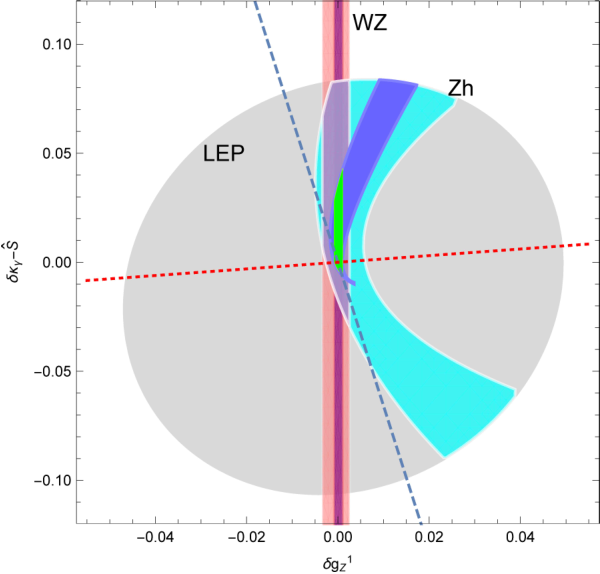
For the universal case, we perform a more detailed analysis. The results are shown in the vs. plane in Fig. 94 for the interesting class of models where [Franceschini:2017xkh]. The direction related to the interference term, i.e., (see Eq. 82 and the second line of Eq. 83) is shown by the dashed blue line, whereas the direction orthogonal to it is shown by the dotted red line. Once the LEP II bounds [432] from the process are imposed, the allowed region that remains is shown by the grey shaded area. We show the results of this work in blue (light (dark) blue for results at 300 (3000) fb-1). The shape of the allowed region arises due to the fact that the interference term vanishes along the dashed blue line and the squared term increases in magnitude as we move away from the origin. This curves the allowed region away from the dashed line as we move away from the origin. The accidental cancellation of the interference term means that our bounds are susceptible to dimension-8 effects along this direction. On the other hand our bounds are more robust and not susceptible to such effects in the orthogonal direction shown by the red dotted line.
| Our Projection | LEP Bound | |
|---|---|---|
As production constrains the same set of operators as the production in Fig. 94, we also show the projected bound from the process at 300 fb-1 obtained in Ref. [Franceschini:2017xkh] (see section 4.1). Only the purple region remains when both these bounds are combined at 300 fb-1. This shrinks further to the green region at 3000 fb-1. A drastic reduction in the allowed LEP region is thus possible by considering the at high energies.
4.3 Novel measurements of anomalous triple gauge couplings6060 60 Contacts: A. Azatov, D. Barducci, J. Elias-Miró, E. Venturini
In this work we are interested in the measurement of the Standard Model (SM) Triple Gauge Couplings (TGCs). This is a classic test of the SM and a possible measurement of deviations from its expectations would signify an invaluable piece of information for the theory beyond the SM. A consistent way to parametrise such possible deviations is through the SM Effective Field Theory (EFT) approach. We are going to consider the SM EFT as defined in [418, 435], in particular we are going to focus on the measurement of the EFT operator , see Table 1, which is associated to the the anomalous triple gauge coupling (aTGC) .
A precise determination of the TGC stems from the measurement of the cross section [436, 421]. Naive dimensional analysis and standard EFT reasoning predicts that the energy scaling of such cross-section is given by
| (86) |
where the first factor accounts for the energy flux of the initial quarks, are the relevant Wilson coefficients, and we have omitted numerical factors. In (86) we have explicitly indicated dimension six squared (BSM62) and SM-dimension six interference terms (BSMSM).6161 61 Note that operators of dimension 7 necessarily violate either baryon or lepton number. We assume the scale of such symmetry violation to be very large and therefore irrelevant for di-boson physics at the LHC. The ellipses in (86) are due to corrections from operators of dimension , which we will neglect. The leading such term is an interference term of the type BSMSM and it is of order .
A closer inspection however reveals that the di-boson production through the dimension six operator has an interference piece with a suppressed energy scaling. Indeed, the energy scaling of such process is
| (87) |
This is a consequence of the helicity selection rules, see [437, 438, 418, 417]. The suppressed energy scaling can be problematic for the correct EFT interpretation of the measurement. Namely, in view of (87), the sensitivity on is largely dominated by the quadratic piece , which is . Furthermore, in this case, the measurements become insensitive to the sign of the Wilson coefficient. The main objective of the present work is to improve the sensitivity to the linear piece BSMSM. We will present two classes of solutions to achieve this goal. Firstly, in section 4.3 we will show that the differential angular cross-section of the process has a large sensitivity on BSMSM compared to the inclusive cross-section. Secondly, in section 4.3 we will show that accounting for extra radiation also results in an improved sensitivity on the leading piece BSMSM. These measurements are specially interesting in a HL/HE phase of the LHC, for which we show the prospects below.
Next we will present two ways to improve the sensitivity to the aTGC by restoring the energy growth
of the interference piece BSMSM of the operator.
Interference resurrection via angular distributions
The first way of enhancing the interference term is by noting that in a collider experiment instead of the process we actually measure a scattering, i.e. vector bosons decay into fermions .
Let us start by considering the differential cross section for the production of the polarised particles 6262
62
We ignore the longitudinal Z polarisation which is sub-dominant at the LHC [439].
| (88) |
where sum runs over intermediate Z polarisations and is the Lorentz Invariant differential Phase Space. Then in the narrow width approximation the leading contribution to the interference, i.e. the cross term in 88, is given by , where is the azimuthal angle between the plane defined by the decaying leptons and the plane defined by the collision and momenta, see Fig. 95. Note that has the energy growth expected from naive dimensional analysis, see Eq. 86. An analogous derivation goes through if we also consider the decay of the W gauge boson. The differential interference term for the process WZ is unsuppressed and modulated as
| (89) |
where are the corresponding azimuthal angles. Integrating 89 over the fermion phase space the interference term vanishes as expected from the discussion above. Since the dependence on the two azimuthal angles is additive, integrating over leads to a differential cross-section that is modulated by and that features energy growth. We will use the result in Eq. 89 to prove the aTGC , with an increased overall sensitivity to both the magnitude and sign of the Wilson coefficient.
Following Ref. [417], we make a few remarks on the experimental measurement of in Eq. 89.
The angle can be determined up to an ambiguity ,
since experimentally we can only measure the charges but not the helicities of the leptons from decay.
The reconstruction of the azimuthal angle in the final state suffers from an ambiguity due to the twofold ambiguity in the determination of the neutrino momentum.
Interestingly, none of these ambiguities affects Eq. 89.
Interference resurrection via jet emission
A second way to resurrect the expected energy growth of the
interference term is based on the observation that the helicity
selection rule holds only at leading-order [418].
So the next-to-leading-order (NLO) effects will necessarily lead to the
enhancement of the interference.
Virtual effects are expected to be suppressed by a factor with respect to the contributions coming from azimuthal modulation discussed in the previous section. A complete study at NLO accuracy for the operator together with its CP-odd counterpart can be found in [435].
Alternatively we will consider processes with an extra hard jet emission, which will improve on the signal over the background ratio.
In this case, since we are dealing with the hard
process,
the same polarisation configuration is allowed both in SM and in the BSM five point amplitude with the insertion. Therefore the interference is not suppressed and the leading quadratic energy scaling is restored by requiring an extra (hard) QCD radiation.
Results
HL-LHC. In order to test the sensitivity of the High-Luminosity (HL) phase of the LHC on the with the proposed solution to the non-interference behaviour we proceed in the following way. We generate with MadGraph5 aMC@NLO [79] parton level events for decaying into a four leptons (electron and muon) final state together with events for the same process where we allow for a jet emission in the initial state. We perform two different analyses (see [418] for more details): an inclusive one where we restrict to events up to \UGeVand do not bin on the variable and an exclusive one where we bin both on the jet transverse momentum and on , where for the latter we define two bins with the threshold . All together the results for the bound on the Wilson coefficient are reported in Fig. 96 as a function of the maximum transverse mass of the system, which allows to have an estimate of the validity of the EFT computation, see again [418] for a detailed discussion 6363
63
These results are obtained by keeping both the linear and the quadratic terms in the cross section determination..
One might wonder if a simulation beyond the parton level accuracy might spoil these results. To this end we have performed a more detailed simulation by showering the events through PYTHIA 8 [79] and simulating the detector response via Delphes 3 [13]. By analysing the density of events in the two azimuthal bins we found that with respect to the parton level case the relative difference is of at most a few %, thus making our parton level analysis solid.
HE-LHC. We now estimate the reach of a future HE phase of the LHC with \UTeV. For these preliminary results we adopt the same binning, both in and in jet transverse momentum, of the previous section. We show the results in Fig. 97. We found a slight increase of order on the reach on . We expect that a dedicated HE analysis will lead to a further improvement of these bounds; this can be done by exploiting in a more efficient way the high energy tails of the differential distributions. In [435] we also present a complete NLO study for the HE-LHC stage.
4.4 Electroweak Precision Tests in High-Energy Drell-Yan Processes6464 64 Contacts: S. Alioli, M. Farina, G. Panico, D. Pappadopulo, J.T. Ruderman, R. Torre, A. Wulzer
The simplest process allowing to set constraints on EFT operators is Drell-Yan di-lepton and lepton-neutrino production at high invariant mass, for concreteness we focus on oblique corrections only, generalisations being rather obvious. These corrections can be parametrised in the electroweak sector by the four oblique parameters , , and . These correspond to four operators that modify the propagators of the and bosons both on the pole ( and ) and off the pole, i.e. on the tails ( and ). Hadron colliders can hardly compete with lepton colliders for pole observable. However, due to the enhancement of the kinematic distributions with respect to the corresponding SM ones at high energy, hadron colliders are particularly suited to study off-pole observables like and . Deviations from the SM proportional to and can be parametrised through the two operators from table 1,
| (90) |
They modify the neutral and charged gauge boson propagators as
| (91) |
Studying the tails of the invariant mass distribution of two leptons and of the transverse mass of lepton-neutrino, one can set constraints on these observables. For details on the procedure see ref. [440], also extended to di-jet and multi-jet analyses in ref.s [441, 442]. The prospect results for the HL-LHC and HE-LHC are shown in fig. 98

4.5 Testing the universal Higgs non-linearity6565 65 Contacts: D. Liu, I. Low, Z. Yin
In this section we motivate precision measurements on the tensor structures of one Higgs couplings with two electroweak gauge bosons (HVV) and two Higgses couplings with two electroweak gauge bosons (HHVV) in HE/HL LHC. There exist special relations between HVV and HHVV couplings in composite Higgs models that are universal, independent of the symmetry breaking pattern invoked in a particular model. These "universal relations" are controlled by a single input parameter, the decay constant of the pseudo-Nambu-Goldstone Higgs boson. Testing the universal relations requires measuring the tensor structures of HVV and HHVV couplings to high precision. In particular, HHVV interactions remains as one of the few untested predictions of the Standard Model Higgs boson, which can be probed through the double Higgs production in the vector boson fusion (VBF) channel at the LHC. Below we summarise the main results. The phenomenological details and theoretical foundation can be found in Refs. [443, 444, 445, 446]
At the leading two-derivative order, the HVV and HHVV couplings in composite Higgs models in the unitary gauge is given by the following simple expression:
| (92) |
where \UGeV, is the decay constant of the composite Higgs boson and . This result is independent of the symmetry breaking pattern of the strong composite sector in the UV, apart from the overall normalisation of , which does depend on the UV model.
At the four-derivative level, we parametrise the HVV and HHVV couplings as follows:
| (93) |
where the definition of the operators and are presented in Table 71 and Table 72. On the other hand, and are Wilson coefficients which depend on six unknowns () in composite Higgs models and on four unknowns () in the Standard Model Effective Field Theory (SMEFT). In the above is the typical mass scale of the new composite resonances. The different Lorentz structures lead to different angular distributions in the decay products and, therefore, can be measured accordingly. At the LHC Run 1, testing the tensor structure of HVV couplings was among the top priorities and gave confidence to the Higgs nature of the 125 \UGeVresonance. (See, for example, Ref. [447].) A similar program for HHVV coupling is currently lacking and should be pursued at HE/HL LHC.
| (NL) | (D6) | |
|---|---|---|
| (1) | ||
| (2) | ||
| (3) | ||
| (4) | ||
| (5) | ||
| (6) |
| (NL) | (D6) | |
|---|---|---|
| (1) | ||
| (2) | ||
| (3) | ||
| (4) | ||
| (5) | ||
| (6) | ||
| (7) | ||
| (8) | ||
| (9) | ||
| (10) |
In general, we have two different Lorentz structure in the HVV couplings:
| (94) |
where and with electric charge conservation implicitly indicated. For HHVV couplings we have:
| (95) |
The ultimate goal then will be to measure these different tensor structures at CLIC.
From Table 71 and Table 72, we can extract relations among and that only depend on the . We call them "universal relations" as they represent universal predictions of a composite Higgs boson, whose nonlinear interactions are dictated by the underlying shift symmetries acting on the four components of the Higgs doublet [443, 444, 445, 446]. Some examples of universal relations involving both HVV and HHVV couplings are:
| (96) | |||
| (97) | |||
| (98) |
These relations depend on one single parameter or, equivalently, . In other words, they can be used to over-constrain the parameter . If the 125 \UGeVHiggs boson indeed arises as a pseudo-Nambu-Goldstone boson, the decay constant as measured from the different universal relations must be consistent with one another.
In order to test the universal relations, it is necessary to measure the tensor structures of HHVV couplings. This is where the HE/HL LHC could have an advantage over circular lepton colliders. At a hadron collider, can be measured from single Higgs decays into four leptons in a fashion similar to the analysis performed in Ref. [447], while measurements on would have to rely on double Higgs production in the VBF channel and the associated production with a boson. The production topology is displayed in Fig. 99.
In Fig. 100 we show the double Higgs production rate in the VBF channel and the associated production channel in a hadron collider as a function of the centre-of-mass energy , adopting the computation done in Ref. [278]. The VBF rate at 13 \UTeVis less than 1 fb, while at 27 \UTeVthe cross-section is about 3 fb, which offers the best chance to probe the HHVV couplings at the LHC.

The analysis of the HHVV coupling is further discussed in the next section 4.6.
4.6 Higgs pair production in vector-boson fusion at the HL-LHC6666 66 Contacts: F. Bishara, R. Contino, J. Rojo
While the dominant production channel of Higgs boson pairs at hadron colliders is the gluon-fusion mechanism, other channels are also of phenomenological relevance. In particular, Higgs pair production in weak vector-boson fusion [448] is interesting since it probes the strength of the Higgs non-linear interactions with vector bosons at high energies. This process can therefore provide unique information to test the nature of the Higgs boson, whether it is a composite or elementary state, and whether or not it emerges as a Nambu-Goldstone boson (NGB) of some new dynamics at the \UTeVscale [40, 449, 450].
The production of Higgs pairs in the VBF channel [40, 449, 451, 452, 453, 454] proceeds via the soft emission of two vector bosons from the incoming protons followed by the hard scattering, with . In the SM, the VBF inclusive cross section at 14 \UTeVis around 2 fb (see Fig. 100), more than one order of magnitude smaller than in gluon fusion. Higher order QCD corrections are moderate () as expected for an electroweak process. Despite the small rate, Higgs pair production via VBF is relevant since even small modifications of the SM couplings induce a striking increase of the cross section as a function of the di-Higgs invariant mass, for instance in models where the Higgs is a composite pseudo-NGB (pNGB) of new strong dynamics at the \UTeVscale [240]. In these theories, the Higgs anomalous couplings imply a growth of the cross section with the partonic centre-of-mass energy, , where is the pNGB decay constant [40]. This enhanced sensitivity to the underlying strength of the Higgs interactions makes double Higgs production via VBF a key process to test the nature of the electroweak symmetry breaking dynamics and to constrain the quartic coupling in a model-independent way.
Here we review the feasibility of measuring and interpreting the VBF Higgs pair production at the HL-LHC in the final state. While QCD multi-jet backgrounds are huge, this final state turns out to be within the reach of the HL-LHC thanks to the unique VBF topology, characterised by two forward jets well separated in rapidity and with a large invariant mass and a reduced hadronic activity in the central region. In addition, the di-Higgs system will acquire a substantial boost in the presence of BSM dynamics, and jet substructure techniques [455, 456, 457] make it possible to fully exploit the high-energy limit and optimise the signal significance.
To describe the deviations of the Higgs couplings with respect to their SM values we follow [449] where a general parametrisation of the couplings of a light Higgs-like scalar to the SM vector bosons and fermions was introduced. In this formalism, assuming that the couplings of the Higgs boson to SM fermions scale with their masses and do not violate flavor, the resulting effective Lagrangian is given by
| (99) |
where denotes the Higgs potential,
| (100) |
The parameters , , , , and are in general arbitrary coefficients, normalised so that they equal 1 in the SM. In this contribution we focus on the determination of by means of di-Higgs VBF production in the final state.
Analysis strategy
Signal and background events are simulated at leading-order (LO) by means of
matrix-element generators and then processed through a parton shower (PS).
The dominant background is given by QCD multi-jet production,
while other backgrounds, such as top-quark pair production and
Higgs pair production via
gluon-fusion, turn out to much smaller.
After the parton shower, events are clustered with
FastJet v3.0.1 [15] using the
anti- algorithm [14] with a jet radius .
The resulting jets are then processed through a -tagging algorithm,
where a jet is tagged as -jet with probability
if it contains a -quark with \UGeV.
In order to account for -jet mis-identification (fakes),
jets which do not meet this requirement
are also tagged as -jets with probability or
depending on whether they contain a -quark or not.
Only events with four or more jets, of which at least two
must be -tagged, are retained at this stage.
Subsequently to -tagging, events are classified through a scale-invariant tagging procedure [456, 457]. This step is crucial to efficiently reconstruct the Higgs boson candidates and suppress the otherwise overwhelming QCD backgrounds while at the same time taking into account all the relevant final-state topologies. The basic idea of this method is to robustly merge three event topologies – boosted, intermediate and resolved – into a common analysis. This is particularly relevant for our study given that the degree of boost of the di-Higgs system strongly depends on the deviations of from its SM value.
Acceptance cuts to match detector coverage are applied to signal and background events. We require the of both the light and -tagged jets to be larger than 25 \UGeV, while the pseudo-rapidities of light and -tagged jets, and , are limited by the coverage of the forward calorimeters and by the tracking region where -tagging can be applied respectively. We also impose a set of selection cuts tailored to the VBF topology which is characterised by two forward and very energetic jets with little hadronic activity between them. In particular, we cut on the rapidity separation and the invariant mass \UGeVof the two VBF-tagging jets, and impose a central jet veto (CJV) on the hardest non-VBF light jet in the central region. The VBF tagging jets are defined as the pair of light jets satisfying the acceptance cuts with the largest invariant mass . Moreover, a CJV cut is imposed in VBF analyses to veto light jets with pseudo-rapidity lying between those of the VBF-tagging jets, , above a threshold of 45 \UGeV.
Figure 101 (right) shows the distribution after all analysis cuts for both for the signal (SM and ) and the total background. For , the crossover between the resolved and boosted categories takes place at \UTeV, although this specific value depends on the choice of the jet radius [456]. Unsurprisingly, we find that background events are always dominated by the resolved topology. The decomposition of the total background in terms of individual processes as a function of is shown in Fig. 101 (left), where each component is stacked on top of each other. We see how the background dominates for large while the one is instead the most important for small .
| Cross-sections (fb) | |||||
| Acceptance | VBF | Higgs reco. | \UGeV | ||
| \multirow3* \UTeV | Signal SM | 0.011 | 0.0061 | 0.0039 | 0.0020 |
| Signal | 0.035 | 0.020 | 0.017 | 0.011 | |
| Bkgd (total) | 569 | 47 | |||
The cross-sections after the successive application of the acceptance, VBF cuts, and Higgs reconstruction cuts for signal events (SM and ) and for the total background is shown in Tab. 73. We find that the VBF di-Higgs signal in the SM is rather small already after the basic acceptance cuts. However, the signal event yield is substantially increased for as illustrated by the benchmark value of leading to more than a factor 3 (5) enhancement compared to the SM after the acceptance (all analysis) cuts. The fact that this cross-section enhancement for the scenario is more marked at the end of the analysis is not a coincidence: our selection cuts have been designed so as to improve the sensitivity to by increasing the signal significance in the large- region. Note however that even after all analysis cuts the background is still much larger than the signal (either SM or ) at the level of inclusive rates. It is only by exploiting the large- region that the former can be made small enough to achieve high signal significances.
Projections for the HL-LHC
Following the analysis strategy outlined in the previous section,
we can now estimate the expected precision on the
determination of the coupling at the HL-LHC.
In the left panel of Fig. 102 we show the
posterior probabilities for at 14 \UTeV,
from where we can assess the expected precision
its measurement at the HL-LHC assuming SM couplings.
The corresponding 68% probability intervals for the determination of at the HL-LHC
are are listed in Table 74 for two different
scenarios for the background cross section.
| 68% probability interval on | ||
|---|---|---|
| LHC14 | [, ] | [, 0.48] |
| HL-LHC | [, 0.19] | [, 0.20] |
From Table 74, we find that the coupling, for which there are currently no direct experimental constraints, can be measured with a precision of around at the HL-LHC. It is interesting to compare these results with the experimental precision expected on the fiducial VBF di-Higgs cross section after all analysis cuts, expressed in terms of , the signal strength parameter normalised to the SM result We find that the 95% CL upper limits on for the nominal background cross section is with 300 fb-1, and at the HL-LHC. This result highlights that the high precision expected on can obtained despite the loose constraints expected on the VBF di-Higgs cross section itself.
The results of Table 74 have been obtained by making full use of the information contained on the di-Higgs invariant mass distribution . However, the EFT expansion might break down at large enough values of , corresponding to large partonic centre-of-mass energies, and some assessment on the validity of our procedure is thus required. In particular, results can be consistently derived within the EFT framework only if the new physics scale is larger than the largest value of included in the analysis. Constraining requires making assumptions on the structure of the UV dynamics extending the SM [458]. For example, for the case where the new physics is characterised by a single coupling strength and mass scale [40], one expects , so that for maximally strongly-coupled UV completions (with ) it is possible to derive the upper limit which connects with the new physics scale . The validity of the EFT can thus be monitored by introducing a restriction , and then determining how the sensitivity on varies as a function of [458]. The precision on is shown in Fig. 102 (right) as a function of , where the grey area indicates the region where . As expected, increasing leads to stronger constraints. We therefore find that in the kinematic region accessible at the HL-LHC the EFT description of the di-Higgs VBF process should be valid.
4.7 Higgs Couplings in High-Energy Multi-boson Processes6767 67 Contacts: B. Henning, D. Lombardo, M. Riembau, F. Riva
In this section, based on Ref. [459], we present a novel program to test the Higgs couplings off-shell and at high-energy, via their contributions to the physics of longitudinally polarised gauge bosons. We will show that this program is potentially competitive with on-shell measurements, but it also offers endless opportunities of refinements and improvements.
Our leitmotiv is that any observable modification of a SM coupling will produce in some process a growth with energy. In some sense, this is obvious: since the SM is the only theory that can be extrapolated to arbitrarily high-energy, any departure from it can have only a finite range of validity, a fact that is made manifest by a disproportionate growth in some scattering amplitude. Theories with a finite range of validity are, by definition, EFTs; for this reason the best vehicle to communicate our message is the EFT language where deviations on Higgs couplings come from the operators , etc. We stress nevertheless that at, tree level, the very same conclusions can be reached in the framework [42] or in the unitary-gauge framework of Ref. [45, 419].
The operators of that we will be interested on have the form , with a dimension-4 SM operator (i.e. kinetic terms, Higgs potential, and Yukawas) times
| (101) |
where is the physical Higgs boson and are the would-be longitudinal polarisations of - and - bosons. In this contribution we focus on the last two terms, and study processes with longitudinal gauge bosons instead of processes with an on-shell Higgs; we dub this search strategy “Higgs without Higgs” - HwH in short [459]. For each modification of a Higgs coupling we identify a process where couplings different from the SM ones induce a high-energy growth in the amplitude with respect the SM,
| (102) | |||
| (103) | |||
| (104) | |||
| (105) | |||
| (106) |
where (similarly a generic longitudinally polarised final state) and any (longitudinal or transverse) vector, including photons. In the following paragraphs we explore these processes in turn and provide a first estimate of the potential HwH reach at the HL-LHC in comparison with the reach from Higgs couplings measurements. Our results are based on leading order (LO) MadGraph simulations [79], where the Higgs couplings have been modified using FeynRules [460] and checked against the model of Ref. [461].
The top Yukawa. Modifications of the Yukawa coupling of the Higgs boson to top quarks is reputedly difficult to measure on the resonance [164]; however, an anomalous top quark Yukawa induces a quadratic energy growth in the five point amplitude involving a bottom quark, a top, and three longitudinal bosons . This amplitude leads to a process with a final state consisting of a top quark, a forward jet and two longitudinally polarised vector bosons in the final state.6868 68 See also Ref. [462] that studies final states which exhibits linear -growth with modifications of the top-Yukawa.
The top carries a large transverse momentum due to the hardness of the process, which makes it a good discriminator. We consider two categories, for \UGeV. A forward jet with , \UGeVand \UGeVis required. The signal is classified by counting the number of extra leptons reconstructed in the event. The following table shows the number of signal events at the 14 \UTeVHL-LHC with 3000 fb-1, for \UGeV/ \UGeV,
| Process | 0 | 1 | |||
|---|---|---|---|---|---|
| 3449/567 | 1724/283 | 216/35 | - | - | |
| 2850/398 | 1425/199 | - | 178/25 | - | |
| 3860/632 | 965/158 | 273/45 | - | 68/11 | |
| 2484/364 | - | 351/49 | - | (12/2) |
The categories with two or more leptons have small background. The largest source of background for the hadronic modes comes from where a pair is taken to reconstruct a -boson. The initial cross section is approximately six orders of magnitude bigger than the ones we are interested in, but we have verified that simple cuts on the invariant mass of the pair, on the rapidity of the forward jet, on , and on the separation between the and the , as well as vector boson tagging techniques [463], can reduce this background to a level that is comparable with the signal.
We broadly parametrise this and other backgrounds by a uniform rescaling of the SM signal expectation in each bin (so that for we add an irreducible background equal to the SM signal in each channel), and show the estimated reach in the left panel of Fig. 103. The dashed grey lines compare our results with those from Higgs Couplings measurements (see section 2. For illustration we also show results that focus on channels with at least 2 leptons with a dashed purple line: here the backgrounds are much smaller. The large number of events left in the zero and one lepton categories makes it possible to extend the analysis to higher energies, where not only the effects of the energy growth will be enhanced, but also the background reduced.
The Higgs self coupling. Measurements of the Higgs self-coupling have received enormous attention in collider studies. In the di-Higgs channel at HL-LHC precision can reach at 95%C.L. [312] using the final state. Here we propose the processes of Eq. (103) with VBS scattering topology and a multitude of longitudinally polarised vector bosons. The modified coupling , or the operator , induces a linear growth with energy w.r.t. the SM in processes with final state, and a quadratic growth in processes with . For the former, the same-sign with leptonic decays is particularly favourable for its low background: two same-sign leptons (2ssl) and VBS topology offers a good discriminator against background, allowing for decays. For illustration we focus on this channel in which the SM gives events. Backgrounds from enter with a mis-identified lepton, but it can be shown that they can be kept under control with the efficiencies reported in [464] and with VBS cuts on the forward jets. A potentially larger background is expected to come from fake leptons, but the precise estimation of it is left for future work.
The results -shown in the centre panel of Fig. 103- are very encouraging: this simple analysis can match the precision of the by-now very elaborate di-Higgs studies. There are many directions in which this approach can be further refined: i) including the many other final states, both for the vector decays and for the Higgs decay ii) including the -growing topologies, iii) taking into account differential information. Moreover, the process studied grows only linearly with energy w.r.t. the SM amplitude with transverse vectors in the final state, but it grows quadratically w.r.t. the SM final states, so iv) measurements of the polarisation fraction can improve this measurement.
Higgs to . These decay rates are loop-level and small in the SM: their measurement implies therefore tight constraints on possible large (tree-level) BSM effects, which in the EFT language are captured by the operators .6969 69 The same operators also affect the couplings to and . The same qualitative analysis can be performed with focus on the and vertices, but we prefer to work here with the gauge invariant operators. These also enter in high-energy VBS eq. (104), and they represent a beautiful additional motivation (together with , see below) to study these processes, which at present are often interpreted in the context of anomalous quartic gauge couplings (QGC) [465], corresponding to dimension-8 operators.
We perform a simple analysis of vector boson scattering (VBS) with final states. For the first three we use the usual cuts on the forward jets: , \UGeVand \UGeV[466]. A kinematic variable that captures the hardness of the process is the scalar sum of the of the vector bosons, and therefore we bin the distribution in bins of 250 \UGeVup to 2 \UTeV. For the final state, we follow the analysis for aQGC of [467].
The combined results are displayed in the right panel of Fig. 103, for fully leptonic, semi-leptonic and fully hadronic decays, for backgrounds where, as explained above, corresponds to an additional background of the same order as the SM. Note that we translated the constraints on to the . We find that the final states provide the best reach. For comparison, the individual reach from HL-LHC measurements of HC (section 2) is shown by the black error bars. These clearly offer an unbeatable sensitivity in the direction; the direction is however less tested, and our simple analysis of high-energy probes shows promising results.
Higgs to . It is known that modifications of the tree-level and SM couplings (assumed here to be controlled by a unique parameter, corresponding for instance to in the SILH basis [40]) imply a quadratic -growth in longitudinal VBS. This is discussed in detail in Ref. [449] (and [450] for linear colliders), where it is pointed out that, in the SM, the longitudinal component is suppressed by an accidental factor , which is equivalent to a very large irreducible background. This motivated studies of VBS pair production instead, see [448], finding at , , comparable to from HC.7070 70 The authors of [448] assume separate couplings of the vector bosons to or ; when the Higgs is part of a doublet, these are proportional. Moreover, the numbers we report here are indicative: both HC measurements and the di-Higgs analysis have optimistic and pessimistic scenarios in which these numbers might differ.
Higgs to . This coupling modifies the main production mode at hadron colliders and is, therefore, very well measured. The most interesting high-energy process that can be associated with this coupling is , which has been discussed in Refs. [468, 469, 470]. Using the results from Ref. [468] we estimate HwH versus HC reach at the end of the HL-LHC, in particular we have considered a scenario with and one without the background and three different decay channels . We find that
| HC: | (107) | ||||
| HwH: | |||||
| HwH |
where the numbers stand for the fully leptonic / semi-leptonic / fully hadronic channels.
The partonic process represents here the main irreducible background, as it does not interfere with our amplitude with longitudinal polarisation. Its reduction would constitute an important aspect of HwH analyses. Notice that, unfortunately, in the SM the process is extremely suppressed at high-, to the benefit of the transverse one, see Ref. [471]. This implies that the interference is also suppressed.
Despite these difficulties, which might be overcome in more refined analyses (along the lines of [417, 418]), the high- results remain competitive in the semi-leptonic and fully hadronic channels, assuming that the background from can be efficiently suppressed.
In summary, the preliminary results are very positive, especially given the potential of improvements that we foresee. Simple cut-and-count analyses were shown, in some cases, to match the precision of sophisticated Higgs Coupling measurements. For instance, the channel with leptonic decays, allows a precision comparable to di-Higgs production in measuring the Higgs self-coupling. Similarly, modifications of the top Yukawa can be measured in the many final states to a precision in the ballpark of Higgs coupling measurements. VBS processes and at high-energy offer further alternative possibilities to test the Higgs coupling to electroweak gauge bosons and to gluons, respectively.
4.8 Dimension-6 EFT effects on Vector Boson Scattering at high energies7171 71 Contacts: R. Covarelli, R. Gomez-Ambrosio
In this note we assess the sensitivity of vector boson scattering (VBS) processes to different dimension-6 () operators. We focus here on the final state, decaying to 4 charged leptons. This experimental channel, currently statistically limited at the LHC [472], will become more interesting at the HL-LHC because of the attainable selection purity. The full reconstruction of the final states also gives access to cleaner observables with respect to final states involving bosons, where neutrino 4-momenta must be inferred using approximated methods. This analysis can nevertheless be repeated analogously to other VBS final states.
In [473] we studied the purely electroweak component of the process, referred to as VBS(ZZ). Sensitivity to several operators has been demonstrated, as well as the impact of such EFT contribution on the VBS cross-section and triple and quartic gauge couplings (TGCs and QGCs).
Here we update predictions for the HL-LHC setup and show the kinematic distributions for a handful of relevant operators. For the parametrisations we use the Warsaw basis from [41], following the notation and classification from [474]. Other technical details can be found in the original publication [473].

Effective Field Theory parametrisation
We consider the standard SMEFT parametrisation of eq. (1).7272
72
In particular, we assume CP symmetry, neglecting the CP-odd operators since their impact on VBS cross-sections and differential distributions is negligible. However it is well known that certain variables of these processes (namely spin correlations and polarisations) can be sensible to CP-violation. Further, the SMEFT amplitudes and cross sections can be parametrised as
| (108) |
| (109) |
Here, we assume the linear contribution (red) of the EFT effects to be leading. Analysis of the quadratic terms and the interference terms (both in blue) will be subject of further studies. In particular, are commonly associated with quartic gauge couplings and such contribution, albeit sub-leading, would represent some added value to the linear prediction.
Definition of the fiducial region
The VBS(ZZ) process has a very peculiar experimental signature, with two energetic forward jets and 4 identifiable charged leptons ( or ).
The electroweak component of the process is defined and isolated through some experimental cuts. The ones used in the CMS analysis (in the measurement of the fiducial cross-section) can be found in [472]. Here we define a similarly VBS-enriched region, with a relaxed selection:
| (110) |
EFT analysis
In tables 75 and 76 we show the sensitivities to different operators of the VBS(ZZ) process, as well as of its main background at LHC: the di-boson production channel from quark-antiquark annihilation associated to gluon radiation (studied in depth by CMS for LHC runs I and II in [475], QCD(ZZ)).
Further, in figure 105 we show differential distributions for a subset of operators. In particular we chose the three operators that directly affect triple and quartic gauge couplings, with the following notation, which differs from that of table 1,
| (111) |
However, as reported in tables 75 and 76, there are other relevant operators for the VBS process, for example , the 4-lepton operator that affects , or that enters the boson propagator. More details can be found for example in [476].
Figure 105 should be interpreted as follows: we select one paradigmatic operator (for example ), and see how much does its interference term affect the VBS and di-boson signals ( in this case). As the VBS(ZZ) cross section is still mostly unconstrained experimentally, while the QCD(ZZ) has a uncertainty in the 2-jet bin [475], we know the bounds within which we can vary this coefficient. If we assume for example a positive interference with the total cross-section, we observe that such a small contribution to the total cross-section can represent a large modification in certain bins of the differential distributions. This advantage is twofold: with this procedure we can select the optimal bin(s) for the study and fit of each EFT operator; and, by applying unitarity considerations, we can constrain the values of the Wilson coefficients further. In our example, a contribution of in , still allowed for the total rate, has a large impact on the high energy bins of the distribution.
Conclusions
The VBS(ZZ) and QCD(ZZ) final states, still largely unexplored at the LHC, will be an important source of constraints on EFT operators at the HL-LHC. We have shown the impact that values of Wilson coefficients still experimentally allowed have on differential distributions that are easily accessible experimentally in this channel.


| VBS Signal | Signal strengths (Linear EFT) |
|---|---|
| Class 1: | |
| Class 3: | |
| Class 4: | , , |
| Class 7: | , , |
| , | |
| Class 8a: | () , , |
| , , |
| ZZ Di-boson | Sensitivities (Linear EFT) |
|---|---|
| Class 1: | , |
| Class 3: | |
| Class 4: | , , , |
| Class 7: | , , |
| , | |
| Class 8a: | () , , |
| , , |
4.9 Same-sign WW scattering and EFT applicability7373 73 Contacts: G. Chaudhary, J. Kalinowski, M. Kaur, P. Kozów, S. Pokorski, J. Rosiek, K. Sandeep, M. Szleper, S. Tkaczyk
Although any statistically significant deviation in data from the Standard Model(SM) predictions would be a manifestation of a BSM physics, the question is what we can learn about its scale and its strength before discovering new particles. The appropriate tool for answering this question is the Effective Field Theory(EFT) approach: the information about the scale and the strength of new physics is encoded in the Wilson coefficients of the higher dimension operators, . The usefulness of any EFT analysis of a given process relies on the assumption that only a few higher-dimension terms in the expansion provide adequate approximation to an unknown UV completion. This assumption introduces a strong model-dependent aspect and therefore it is convenient to introduce the concept of EFT “models" defined by the choice of operators and the values of their Wilson coefficients . Our focus is on the proper use of the EFT "models" in their range of validity for the WW scattering in purely leptonic W decay channels where the invariant mass cannot be determined experimentally. A full explanation of the concept is to be found in [477] and here we summarise the main points..
Following a common practice we take one operator at a time setting others to zero, which effectively defines the EFT “model", and consider the process . The EFT “model" can be maximally valid up to the invariant mass of the system , where is the perturbative partial wave unitarity bound in the chosen EFT "model". If the kinematic range at the LHC is greater than , there is necessarily a contribution to observables from the region . Two questions arise:1) what is the discovery region in the space for the chosen EFT "model", 2) if a deviation from the SM predictions is indeed observed, how to verify the chosen EFT “model" by fitting it to a set of experimental distributions and in what range of such a fit is really meaningful?

For a given EFT “model" the unitarity bound is very different for different helicity amplitudes. As we take the value from T-matrix diagonalisation of the and , universally for all helicity amplitudes. The BSM signal of the EFT “model" can be defined as the deviation from SM predictions observed in the distribution of some observable , . A quantitative estimate of the signal can be written as
| (112) |
which comes uniquely from the operator that defines the “model" in its range of validity and assumes only the SM contribution in the region . BSM contribution from the region above may enhance the signal, but it may also preclude proper description of the data in the EFT "model", which makes sense if and only if this additional contribution is small enough compared to the contribution from the validity region. For a quantitative estimate of this contribution we define a second estimate in which all the helicity amplitudes above are assumed to remain constant at their respective values they reach at
| (113) |
For this prescription regularises the helicity amplitudes that violate unitarity at . We adopt the criterion that the EFT “model" is tested for values of when the signals computed from Eq.(112) are statistically consistent within 2 with the signals computed with Eq.(113).
The observability of the EFT "model" predictions imposes some minimum value of , while the description within the EFT "model" imposes some maximum value of such that signal estimates computed from Eqs.(112) and (113) remain statistically consistent. For a finite interval of values is possible, while for the respective limits on depend on the actual value of . It is illustrated in a cartoon plot in Fig. 106, where the white "triangle" is bounded from above by the unitarity bound , from the left by the signal significance criterion and from the right by the consistency criterion. The EFT "model" could be the right framework to describe the BSM signal as long as the “triangle" shown in our cartoon plot is not empty.
Our preferred strategy for data analysis is as follows:
a) Measure distributions that
offer the highest sensitivity to the studied EFT "model",
b) if deviations from the SM are observed, fit the values of
according to
Eq.(113),
c) using the fitted values of and recalculate
templates
according to
Eq.(112),
d) check statistical consistency between estimates based on Eqs.(112) and (113).
Physics conclusions from the obtained values can only be drawn
if such a consistency is found.
Stability of the result against alternative
regularisation methods would provide a measure of uncertainty of the procedure - too much
sensitivity to the region above means the procedure is destined to fail
and that data cannot be described within the chosen EFT "model".
To demonstrate our strategy we considered EFT “models" defined by one-at-a-time dimension-8 operator that affects couplings. Details of the simulation of events for the process (at 14 \UTeVwith 3/ab integrated luminosity) and their processing according to our strategy can be found in [477]. Assuming equal to the respective unitarity bounds, the lower and upper limits for the values of for each dimension-8 operator, for positive and negative values, as well as the applicability "triangles" in the plane for each operator have been calculated. These limits define the (continuous) sets of testable EFT “models" based on the choice of single dimension-8 operators.
Following the above strategy we have calculated the expected reach for the dim-8 operator at the HE-LHC and compared it with the obtained reach for the HL-LHC (14 \UTeV) from Ref. [477], assuming in each case an integrated luminosity of 3/ab. Fig.107 shows the respective “EFT triangles". It is evident that increasing the proton energy allows to explore much lower values of the Wilson coefficients, with lower limits for a 5 BSM discovery being shifted by as much as almost an order of magnitude. On the other hand, the upper limit on consistent EFT description shifts likewise by a similar amount. This is due to the fact that by increasing the collision energy more and more events come from the region, where and therefore shrinking the range of Wilson coefficients that satisfy our consistency criterion. Overall, the area of the actual “EFT triangle" does not get significantly larger for 27 \UTeVcompared to 14 \UTeV, even when viewed in a log scale.
To summarise: we have analysed the physics potential of "EFT models" defined by the choice of single dimension-8 operators in the same-sign WW scattering process in the purely leptonic decay modes. We argue that usage of EFT “models" in the analysis of purely leptonic decay channels requires bounding the possible contribution from the region , no longer described by the “model", and ensuring it does not significantly distort the measured distributions compared to what they would have looked from the region of EFT validity alone and propose a data analysis strategy to satisfy the above requirements. We find that the "triangles" turned to be rather narrow, even when going from 14 to 27 \UTeVof beam energy . This result reinforces our former conclusion that study of BSM effects by means of varying single Wilson coefficients has little physics potential and future data analysis should be rather focused on simultaneous fits of many operators to the combined data from all VBS processes. We find this conclusion to hold equally regardless of the actual beam energy.

Acknowledgements: Work partially supported by the National Science Centre (Poland) grants DEC-2015/18/M/ST2/00054, DEC-2016/23/G/ST2/04301 (SP), DEC-2015/19/B/ST2/02848 (JR) and HARMONIA project UMO-2015/18/M/ST2/00518 (JK) as well as the COST Action CA16108. ST is supported by Fermi Research Alliance, LLC under Contract No. De-AC02-07CH11359 with the US DoE. The work of PK has been supported by the Spanish MINECO project FPA2016-78220-C3-1- P (Fondos FEDER).
5 Higgs boson mass and width7474 74 Contact Editors: Z. Liu, M. Xiao
5.1 Theory review7575 75 Contacts: F. Caola, R. Röntsch
The total decay width is an important property of the Higgs boson, as it contains information about the interactions of the Higgs with all other fundamental particles, and is predictable both in the Standard Model and its extensions. Therefore, measuring this property is an important part of Higgs studies. Direct measurements of the Higgs width are very challenging at hadron colliders, as these require a scan of the invariant mass profile of the Higgs decay products. This is limited by detector resolution to roughly , which is three orders of magnitude larger than the SM prediction of . Current LHC measurements have already attained this level of precision. Although no explicit projection has been made, it is expected that the direct method will only be able to constrain the Higgs width to times the SM value.7676 76 Lower bounds on the Higgs width can be obtained from lifetime measurements.
Given this situation, there has been considerable interest in devising indirect probes of the Higgs width. In general, a standard Higgs analysis in the decay channel measures the production cross section times branching ratio, and is thus only sensitive to a combination of the coupling and the width. Schematically,
| (114) |
where and are the couplings that enter the Higgs production and decay channels, respectively. An independent measurement of the couplings and the decay width is therefore not possible from such analyses. The idea behind all indirect determinations of is to find an observable whose dependence on and is different from Eq. (114), which allows one to lift the coupling/width degeneracy. Indirect determinations can be broadly separated in two classes: on-shell methods, which rely on interference effects on the Higgs resonant peak, and off-shell methods, which combine on-peak and off-peak information. In the following, we provide a quick overview of these methods, emphasising their strengths and weaknesses.
The starting point of the on-shell methods [478, 479, 480, 481] is the observation that measurements in the decay channel receive a contribution both from the signal process and from the continuum background , and the two interfere. Schematically, the amplitude for the process can be written as
| (115) |
where is the signal part and is the background contribution. This leads to
| (116) |
Here, , but , so a combined determination of the signal and interference contributions can lift the coupling/width degeneracy of Eq. (114), thus giving access to . For this method to be effective, one needs to consider channels where the interference is large. The best candidate is the channel: indeed, in this case both the production and the are loop induced, as is the continuum contribution . This implies that at least naively there is a loop enhancement factor in the interference w.r.t. the pure signal, thus making the former noticeable.
The real part of the interference in Eq. (116) is anti-symmetric around the Higgs peak, so it does not affect the total rate. However, it leads to a distortion in the shape of the distribution around the Higgs peak, which in turns translates into a slight shift in the reconstructed Higgs mass [479]. The size of this mass shift is proportional to the interference contribution, whose dependence on couplings and width is different from Eq. (114). A measurement of the mass shift then allows for a determination of . This can be done for example by comparing the mass extracted in the channel with that determined in the channel, where these interference effects are negligible. However, even if the channels lead to a very good mass determination once high enough statistics have been accumulated, extracting the mass shift from a vs comparison introduces additional systematics. One way to circumvent this issue is to consider only the decay mode and to compare different kinematic regions, although detailed systematic studies within this approach have not yet been done. This is possible since the interference is strongly dependent on the transverse momentum of the Higgs [480]. In particular, hard radiation tends to lessen this effect somewhat. Another candidate for a reference mass could be obtained from studying Higgs production in association with two hard jets. Indeed, in this case there are cancellations between the and contributions and the net result for the interference is very small [482]. Theoretical predictions for the mass shift are under good control, with the interference being known to NLO in QCD [480, 483, 484] and matched to parton shower [161, 485]. It turns out that radiative corrections deplete the interference contribution somewhat. Although it is well known that higher order corrections are important for Higgs physics, for this analysis the main limitation comes from experimental systematics, namely the detector response, which must be properly modelled to extract the interference contribution from the measured mass shift. In the SM, the mass shift at the LHC is rather small, . This implies that it will be extremely difficult for this method to access the region . Detailed projections at the HL-LHC can be found in Sec. 5.5.
The imaginary part of the interference [480, 481] in Eq. (116) is symmetric around the Higgs peak, so it leads to a change in the rate. Unfortunately, because of helicity conservation this imaginary part is highly suppressed at LO. Higher order corrections provide a new mechanism to generate an imaginary part, lifting this suppression [480]. However, because the bulk of the interference effectively enters at NLO, the anticipated loop enhancement factor in the interference relative to the pure signal (mentioned above) is not present, and the actual size of the effect is quite small. In the SM, it reduces the total rate by about , which makes it challenging to observe, and the effect is further diluted by additional radiation [481]. Thus this technique requires very good control on the total rate, both experimental and theoretical. To reduce the former, it is profitable to consider cross-section ratios; for example, the to ratio is projected to be measured at the few percent level. However, this introduces additional experimental and theoretical systematics, including theoretical model dependence since one would need to make assumptions about the structure of Higgs couplings. For this reason, it may be advantageous to perform the interference effect extraction in the channel alone, by considering different kinematic regions. As with the real part of the interference, this effect is also quite sensitive to the transverse momentum of the Higgs, with the bulk of the interference effect confined to the small region, as shown in an NLO analysis in Ref. [481]. However, since the interference is essentially an NLO effect, as discussed above, the residual theoretical uncertainty at this order is still quite sizeable. Moreover, a fine-grained comparison of the low and high Higgs regions requires very good theoretical control. For the former, this is notoriously complicated as several different effects are at play, see e.g. [486] and references therein for a recent discussion of this point. Because of this, assuming a few percent experimental accuracy, the width extraction from this method would be limited by theoretical uncertainties. Although computing higher order corrections for this effect is well beyond our current ability, it is reasonable to assume that the situation will improve on the HL/HE-LHC timescale, along the lines described in Section 2.2. Currently, it is expected that this technique will lead to bounds of the order , see section 5.4 for details.
The main advantage of the on-shell width determinations discussed above is that they require minimal theoretical assumptions on potential BSM effects. This is because couplings are extracted at the same energy scale, ideally from the same process. However, since interference effects scale like at the first power, the constraints on the width are relatively mild. Indeed, if one assumes that the on-shell rates are kept fixed, a linear dependence on the coupling translates into a square root dependence on the width.
Another option to constrain the width is off-shell methods [487, 488, 489, 490], which are based on the following observation. Schematically, the cross section can be written as
| (117) |
On the resonant peak, this leads to the usual relation in Eq. (114). Typically, most of the cross section is concentrated there. In the decay channel though there is a sizeable contribution from the off-shell region [487]: indeed, Higgs decay to vector bosons is strongly enhanced at high energy. In the far off-shell region, Eq. (117) reduces to . Assuming that the on-peak rates are kept fixed, this quadratic dependence on the couplings translates into a linear dependence on , allowing this quantity to be constrained by a comparison of on- and off-shell rates.
However, it is important to stress that to extract from off-shell measurements one has to assume that on-shell and off-shell couplings are the same. Since the two are evaluated at very different energy scales, this introduces a theoretical model dependence that is not present in the on-shell methods. Indeed, there are several new physics scenarios where BSM effects decorrelate on- and off- shell couplings, see e.g. [468, 491, 492, 493] and sections 4.7, 4.8 where some of these effects are discussed explicitly. These include, for example, new light degrees of freedom coupled to the Higgs, additional Higgs states, or anomalous couplings. Therefore, to constrain the width using an off-shell analysis, it is important to perform complementary measurements to control potential BSM effects. This was studied in detail for the case of anomalous couplings in [494]. Projections at the HL-LHC will be presented in section 5.3. In general, off-shell measurements offer the opportunity to investigate Higgs interactions at high energy scale, thus leading to interesting information that is not limited to the width extraction. For example, in combination with measurements of boosted Higgs, and , an off-shell analysis can help lifting the degeneracy between and couplings [468]. The off-shell program will clearly benefit from the increased statistics and energy of the HL/HE upgrade. For example, this would allow for off-shell studies in the VBF production mode [495]. Although the rate here is very small, by looking at same-sign vector boson final states one can significantly reduce backgrounds. Although it is estimated that HL-LHC measurements in this channel would lead to constraints at the same level of current ones in the channel [495], the completely different production mechanism makes them complementary to the constraints, thus allowing for a less model dependent interpretation. Aside from these considerations, it is interesting to study the potential of future LHC upgrades to constrain under the assumption that no large decorrelations between on- and off-shell couplings occur. Because of the linear dependence on the width discussed above, such constraints are rather powerful. Indeed, assuming a reasonable reduction in the theoretical uncertainty in the HL-LHC timescale, it will be possible to probe values close to the SM value . Projections under different assumptions for the theoretical uncertainty are reported in section 5.3.
A reliable theoretical description of the off-shell region is non trivial. First, there is a large background, which needs to be properly subtracted to access the signal yield. More important, there is an irreducible continuum background that interferes with the signal process . The interference effect is sizeable and destructive, which is a consequence of the Higgs mechanism ensuring unitarity in the SM. Because of the large interference, it is necessary to have good theoretical control not only on the signal process but also on the continuum background amplitude. This is non trivial, since the process is loop induced, so higher order corrections – expected to be large given the initial state – involve multi-loop amplitudes. Moreover, at large invariant masses, the contribution of virtual top quarks to the amplitude becomes dominant. Its proper description would then require multi-loop amplitudes involving internal massive states, which are extremely challenging to compute. For this reason, exact predictions for the background amplitude are only known to LO in the off-shell region. NLO corrections are known below the top threshold, and only in an approximate form above [496, 497, 498, 499, 500, 501, 502]. Nevertheless, recent developments in numerical techniques [274] make NLO computations for the background feasible in the near future. One subtle point in this discussion is the role of quark-initiated reactions. On the one hand, they appear naturally in the computation of NLO corrections to from initial state splitting. On the other hand this kind of contribution – although separately finite and gauge invariant – only forms a small subset of the whole process at , which are part of the genuine N3LO corrections to the quark-initiated process. Therefore, only including the contribution coming from initial state splitting in the process, although formally possible, may not entirely capture the correct physics. In general, this problem is not particularly relevant because the gluon channel provides the bulk of the contribution. This is however no longer the case if strong requirements on extra jet activities (typical e.g. for analysis) are imposed. Understanding this issue is an interesting theoretical problem, and the high statistics available at the HL/HE-LHC motivates its detailed investigation. Another issue that should be investigated is the impact of electroweak corrections, which can be sizeable at high energy. Once again, although they are currently unknown, it is natural to expect progress in this direction within the HL-LHC timescale.
The modelling of the process is under better control than the background one. Still, since in the far off-shell region the top loop cannot be approximated by a contact interaction, computations are still much harder than in the on-shell region, where such an approximation is justified. As a consequence, exact results are only known to NLO. A full computation of NNLO corrections would require significant advances on current technology, which are however likely to occur in the HL-LHC timescale. It is reasonable to expect [45] that the -factor for the exact theory is rather similar to that obtained from calculations in which the top loop is integrated out. In the absence of an exact calculation, one can use this approximation to estimate rates at the HL/HE LHC.
The HL/HE-LHC upgrade will improve off-shell analysis in several ways. On the one hand, the larger statistics will allow for a better discrimination of the vs background and – crucially – interference. Currently, this is done by using the different kinematic behaviour of these contributions. Clearly, a higher statistical sample would allow for more powerful discrimination. Furthermore, increasing the collider energy would lead to a larger fraction of gluon initiated events w.r.t. quark initiated events. For example, the ratio increases by a factor of roughly 1.5 in the off-shell region when the centre-of-mass energy is increased from 14 \UTeVto 27 \UTeV. Furthermore, the increase in the total rate at the HE-LHC will lead to a significant number of off-shell events in the few-\UTeVregion. This would allow for precise investigations of the Higgs sector in the high-energy region, which could shed light on the unitarity structure of the SM.
5.2 Measurement of the Higgs boson mass7777 77 Contacts: G. Barone, A. Gabrielli
The measurement of the Higgs boson mass by the ATLAS and CMS experiments at the LHC is [10]:
This precision is reached with the two high resolution Higgs boson measurement channels the and . At the LHC Run 2, the precision in the latter channel is already limited by the systematic uncertainty on the photon energy scale. The photon energy response is calibrated using both electrons from Z decays (which requires to be extrapolated from electrons to photons) and radiative Z events reconstructed with two charged leptons and a photon, which is limited by statistics in the transverse momentum range of interest. The most precise measurement is obtained in the and the where the on-shell Z mass constraint can be applied to the system.
Detailed studies of the calibration of the muons, electrons and photons with the very large HL-LHC sample have not been done yet, however it is plausible that the mass of the Higgs boson will be measured with a precision of 10-20 \UMeV, assuming that with the higher statistics the analysis will be further optimised to gain in statistical precision and that systematic uncertainties on the muon transverse momentum scale will significantly improve with the higher statistics.
5.3 Constraints from off-shell Higgs boson production7878 78 Contacts: M. Xiao, U. Sarica
Extracting the Higgs width from off-shell measurements are performed in ATLAS [503] and CMS [271] experiments using LHC Run 1 and Run2 data. The latest constraints on the Higgs width are \UMeVand \UMeVfrom ATLAS and CMS, respectively. Theoretical basis of the measurements is that on-shell and off-shell couplings are the same. Developed on the experimental analyses, the expected precision on the Higgs width at the luminosity of 3000 is given in this section.
The CMS projection adopted the same analysis strategy as defined in the Run 2 analysis [CMS-PAS-HIG-18-002], where the final state is used. Events are selected and put into different categories that are sensitive to ggF, VBF and VH production modes. The invariant mass of the four leptons, matrix-element based discriminant separating the major signal and background events and discriminants sensitive to the width are used in each category. The ratio between off-shell and on-shell event yields and the shape of the observables are sensitive to the Higgs width. To extrapolate to 3000 , event yields are scaled with luminosity. Assumptions on the uncertainties are made, and two scenarios are considered [139]:
- •
“Run 2 systematic uncertainties” scenario (S1): All systematic uncertainties are kept constant with integrated luminosity. The performance of the CMS detector is assumed to be unchanged with respect to the reference analysis;
- •
“YR18 systematic uncertainties” scenario (S2): Theoretical uncertainties are scaled down by a factor of two, while experimental systematic uncertainties are scaled down with the square root of the integrated luminosity until they reach a defined minimum value based on estimates of the achievable accuracy with the upgraded detector.
The projections are shown in Fig. 108. Limits on are given for an approximate S2 in which the experimental systematics are not reduced, while the theoretical systematics are halved with respect to S1. The additional uncertainty applied on the QCD NNLO K factor on the background process is kept the same in this approximated S2 in order to remain conservative on the understanding of these corrections on this background component. It is also noted that the uncertainties on the signal and background QCD NNLO K factors are smaller in the Run 2 analysis [271] than in previous projections using Run 1 data [504]. The expected precision in S2 is \UMeV.
The ATLAS projection [504] is based on the ATLAS Run1 analysis [PhysRevD.91.012006]. final state is used. Events are selected and put in ggF, VBF and VH categories. The invariant mass of the four leptons and a matrix-element based discriminant sensitive to both signal background separation and width variation are used. In the extrapolation to 3000 , event yields are scaled with luminosity and the change in the centre mass of energy. Only theoretical uncertainties are taken into account, as the experimental ones have a negligible impact. The treatment of theoretical uncertainty is close to Run1 analysis, with more conservative ones below:
- •
The k-factor uncertainty for the gg initial state signal, background and their interference is taken as 30%. Based on the latest theory papers, this uncertainty is considered to be conservative, and is 10% is the CMS projection result.
- •
The background to signal k-factor ratio uncertainty, two benchmarks are considered: 10% and 30%.
The expected precision on at 3000 is \UMeVas shown in Fig. 109. It is more conservative than the CMS result, and the cause of it was discussed above.
In conclusion, it is reasonable to believe the realistic precision from ATLAS at 3000 will be better than the number above. Using the CMS numbers, we con estimate that with CMS and ATLAS measurements combined, the precision on the width can reach \UMeV.
5.4 Width from the di-photon interference rate7979 79 Contacts: J. Campbell, M. Carena, R. Harnik, Z. Liu. This manuscript has been authored by Fermi Research Alliance, LLC under Contract No. DE-AC02-07CH11359 with the U.S. Department of Energy, Office of Science, Office of High Energy Physics.
The SM Higgs total decay width can be constrained from the change in on-shell Higgs rates due to interference effects between the Higgs signal and the QCD background [481]. This change in rates requires the existence of a so-called strong phase in the amplitudes, that can be present both in the Higgs signal and in the continuum background, as is the case in the SM. We shall demonstrate that, the different scaling behaviour between the strong phase induced interference and the Breit-Wigner parts of the on-shell Higgs rate may allow the placement of bounds on, or even measurements of, the Higgs boson total width. Both theoretical and experimental uncertainties are the leading limiting factors in this program. On the other hand, without the strong phase induced interference effects, fits to on-shell Higgs rates can only place bounds on the total width by making definite theoretical assumptions [505, 44, 506].
It is useful to write the amplitude for in a form which explicitly factors out the loop-induced couplings to gluons () and photons (),
| (118) |
Both the Higgs couplings and as well as the background amplitude receive absorptive contributions that arise from loops of particles that are sufficiently light to be on shell. The resulting induced phases are usually dubbed ‘strong phases’ in the flavor literature and we will adopt this terminology here.8080 80 Strong phases, which are CP even, get their name because they often arise in flavor physics from QCD dynamics. This is in contrast with CP odd weak phases, e.g., the relative size of the Higgs couplings to versus . In the presence of a strong phase we can write the interference term as
| (119) | |||||
where we have taken and as the signal and background strong phases, respectively. The first term in the square bracket is the contribution to the interference term that does not modify the overall rate upon integration over . The second term is the subject of this work and leads to a modified rate in the presence of a strong phase. For convenience, we define and such that
| (120) |
In the SM the dominant contribution to comes from the phase of the background amplitude at two loops [507, 478]. The signal amplitude also contains a strong phase, mainly due to bottom quark loops. We have performed a calculation of the interference effect that accounts for absorptive effects from both signal and background. In Fig. 110 we illustrate the features of the interference effects. The line shape, the differential cross-section as a function of , is shown for the pure Breit-Wigner (only ), and for the interference contributions and as well as for the sum of both. For visualisation, the interference contribution has been magnified by a factor of 10. In this figure we show the line-shapes obtained including NLO effects with virtual corrections only. After summing over different interfering helicity amplitudes, we obtain averaged strong phases and for the signal and background, respectively.
As a concrete example that demonstrates the potential of this novel effect, without loss of generality we can consider excursions in the flat direction corresponding to,
| (121) |
The total Higgs cross section can then be written as,
| (122) |
The result of a full NLO calculation of the interference effect are presented in Fig. 111, that shows the relative size of the interference effect as a function of the total width, normalised to its SM value, for parameter excursions defined by Eq. (121). 8181 81 For details of the NLO calculation , see the supplemental material with Refs [508, 509, 510, 511, 512, 483, 513, 514, 97, 515, 516, 517, 518]. The variation of the interference effect with the total width is shown imposing a 20 \UGeV-veto, with and without LHC cuts on the final state photons. Since the interference effect is largest at small scattering angles, the photon cuts reduce the expected interference. This small consideration in the SM leads to much bigger differences for . Observe that in the SM the interference contribution is destructive. However, if the sign of were flipped, (), the interference effect would lead to an enhancement of the di-photon rate rather than a suppression. The theoretical scale uncertainty is shown in the bottom panel of Fig. 111 and amounts to about . For example, the interference effect is without photon cuts for SM Higgs.
Although a measurement at the 2% level may be challenging at the LHC, this shows that a precise measurement of the rate can place a limit on the width of the Higgs boson. In this respect a measurement of the ratio of the rate to the rate is a promising route to reduce many of the systematic and theoretical, e.g. PDF and other parametric, uncertainties.
The best measured channels at the LHC, and , provide the most accurate cross section ratio, projected to be measurable at the 4% level [519]. In contrast to single cross section measurements, the precision on this ratio is statistically limited. Keeping the current theoretical uncertainty band in mind, the projected sensitivity of 4% on the ratio of to yields can be translated into an upper limit of 22, 14, and 8 on at 1- level, for low, central and high theoretical expectations on this interference effect, respectively.8282 82 This limit is worse by one order of magnitude than the off-shell Higgs measurement that constrains the Higgs total width [487, 488, 489]. However, unlike the off-shell Higgs measurement, our effect is independent from the assumptions on the high-energy behaviour of the Higgs boson and the absence of new physics contribution in the off-shell region. For more detailed discussion, see e.g., chapter I.8 of the Higgs Yellow Report [45] and Refs. [491, 492]. This assumes that the couplings to photons and bosons maintain their SM ratio and the photon and gluon couplings respect Eq. (121). The Higgs cross section precisions are anticipated to improve by a factor of three or so from statistical improvement at the HE-LHC with 27 \UTeVcentre of mass energy and 15 of integrated luminosity. This can be naively translated into lower and upper limits on the Higgs total width of at 1- level using the central value from our NLO theory calculation.
In summary, we discuss the change in the on-shell rate, due to interference between the Higgs signal and the QCD background amplitudes, as a way to provide a novel handle to constrain - or even measure - the Higgs boson total width. We perform a full NLO calculation at order of the interference effect and find that in the standard model it leads to a reduction of the on-shell rate by . The proposed method for gaining sensitivity to the Higgs boson width is complementary to other methods that have been discussed in the literature. Altogether our study aims at motivating a more thorough examination of Higgs precision physics taking into account the strong phase induced interference effect in different Higgs boson observables.
5.5 Mass shift from the di-photon interference8383 83 Contact: C. Becot
A detailed study of the impact of the phenomenon of interference between the signal process and its irreducible background process has been made in [520]. It will be summarised below.
All the results from [520] have been made with simulated data for the \UTeVdataset. A full-fledged extrapolation to higher centre of mass energies remains to be done. However, the two processes that interfere together, are induced by the same initial state and are at a similar mass scale. All the results are based on a difference between results made with simulated data where the interference have been implemented in the simulation, and simulated data where it is not. In the following, we will therefore consider that any increase of the cross-section with respect to will cancel out in the difference.
The main goal of [520] was a robust estimate of the mass shift induced by the interference between and its irreducible background process within the Standard Model (SM). This was achieved by using the Monte-Carlo generator Sherpa 2.0, that provides a specific plug-in allowing to generate datasets of weighted events, corresponding either to the the signal term ( amplitude), the irreducible gluon-induced background term ( amplitude), their interference term or a any combination of these processes. The Feynman diagram describing the different processes involved are given in fig. 112.

It was the first time that Sherpa 2.0 was used in an analysis, and in particular the only time its interference module has been used. The distribution of the di-photon pair transverse momentum () has been studied in detailed, as it is a preliminary requirement to be able to recast the mass analysis described in [521]. To get the best match of the distribution between this simulation and the state of the art estimates, Sherpa 2.0 had to be tuned. This was done by varying the parameter that controls the scale at which the parameter is evaluated during parton shower evolution for the initial state. Simulated data samples were generated at several values of this parameter and compared to prediction for the Higgs boson transverse momentum from HRes2.0. The value of for which both predictions were agreeing the best has been kept for the simulations used for the final result. The distributions of obtained for a simulation of the background has been compared between ResBos and Sherpa2.0 for the best value of . They were found to be in reasonable agreement.
Then large samples of weighted signal (S) and interference (I) events were simulated. The background component was determined using a data-driven method (B). The background functions described in [521] were re-used, and they were fitted to the \UTeVdataset. This allowed to construct two varieties of simulated templates, one that was made of and the other of . These samples were then folded by the energy resolution and photon efficiencies used in [521] to mimic the detector simulation. The di-photon mass distributions induced by these different terms can be found in fig. 113. The Higgs boson mass () is measured separately on both templates, giving the values of including the impact of interference (), and without (). Then the impact of the interference term itself on is determined as
| (123) |

Several uncertainties have been considered. First a non-closure of 3 \UMeVhas been observed while measuring from the S+B simulated sample, and is propagated as an experimental uncertainty. The only other experimental uncertainty stems from the choice of background function, and has been estimated at 3 \UMeVby trying different background functions.
For theoretical uncertainties we considered both scale variations as well as K-factor variations, as we will describe now. The renormalisation and factorisation scales were varied by a factor of 2, between and (the nominal value is ). The resummation scale itself was varied between and . Samples were re-generated at these different values of the scales for S and I, and the value of was re-evaluated. This gave a small uncertainty of \UMeV, which can be explained by the migration of events between transverse momentum categories that leads to a cancellation of these variations in the difference .
The signal K-factor () has been varied by 0.1, between and . The background K-factor is not known, and it was decided to vary it between 1 and . The recipe gave an uncertainty of \UMeV, which is the dominant uncertainty. Constraining could lead to a huge improvement, but it requires to separate the component from the inclusive production. This is expected to be complicated but might be achieved by the study of angular distributions in .
This study conducted to the following estimate of the Higgs boson mass shift induced by the interference process within the Standard Model :
| (124) |
The mass shift was also determined for larger widths, in the specific scenario where the width is modified but the expected number of events around the di-photon peak (S+I), is not. The mass shift was determined to be \UMeVfor \UMeVand \UMeVfor \UMeV. By the end of HL-LHC such deviations could be probed by comparing the mass measured in the high-precision channel and the one measured in . The following difference :
| (125) |
will be largely dominated by the systematic uncertainty on . Assuming it is at the same level than the one of Run 2 [522], it would lead to an uncertainty on the measured of 290 \UMeV, hence a shift of 580 \UMeVcould be excluded at 95% C.L. Also assuming that scales linearly with the Higgs boson width, it would allow in this naive model, to set upper limits on the Higgs boson width at \UGeVat 95% C.L.
This is only using the difference between the Higgs boson mass measured in its 4 leptons decay channel and the one measured in its di-photon decay channel. Now, it is also known that the interference term will have a bigger impact in some parts of the phase space where the signal to background ratio is smaller. This is for instance the case at low , and it could be used to carry out the same inference internally in the channel, comparing the masses measured in two (or more) bins. A full-fledged prospect study of this analysis remains to be done, as the only attempt carried out so far [523] suffered from large mis-modellings of the kinematic distributions and of the cross-sections. The success of such an analysis will rely on very precise predictions for the kinematic distributions, which is not yet available. This will require the development of new higher-order calculations and resummed predictions, and could be helped by the development of new Monte-Carlo tools using better showering algorithms.
6 Invisible decays of the Higgs boson8484 84 Contact Editors: A. Magnan, B. Nachman, T. Robens and T. Stefaniak
Invisible decays of the Higgs boson are a generic prediction of new physics models that feature a light dark matter (DM) particle which couples directly or indirectly to the Standard Model Higgs field. The invisible branching ratio in the SM is very small (0.1%) so any observable rate would be evidence for physics beyond the SM. LHC searches for this signature require the Higgs boson to be produced in association with a taggable object, most importantly, a -boson, extra forward jets (as appearing in the vector boson fusion process), or a single high- jet. Furthermore, the invisible Higgs decay to the DM particles inevitably suppresses the branching fractions for the Higgs decays to SM particles. This — along with possible model-dependent alterations of the Higgs couplings — leads to a modification of the LHC Higgs signal rates of channels with SM final states with respect to their SM expectation, which can be probed with precision Higgs measurements.
In so-called Higgs portal models the SM Higgs field acts as a mediator between the visible SM sector and a hidden DM sector. Commonly, an additional symmetry is introduced that prohibits interactions of single hidden sector fields with SM fields, thus allowing only pair production of hidden sector particles and rendering the lightest hidden sector particle a stable DM candidate. The Higgs portal and its generalisation to other non-SM Higgs bosons are found in many BSM scenarios (see e.g. Refs. [524, 525, 526, 527] and [528, 529, 530, 531, 532, 533] for models with and without supersymmetry).
The invisible decay of the Higgs is experimentally challenging because the missing transverse energy spectrum is relatively soft, where resolution and pileup effects are non-negligible. The issues associated with pileup, both from pileup jets and from pileup-induced resolution degradation, will only become more severe beyond Run 3. Significant recent advances in constituent-based pileup mitigation techniques will likely play a key role in maintaining and possibly improving the MET performance [534, 535, 536, 537, 538]. Furthermore, lepton identification and pileup jet rejection will both improve with the increased tracking acceptance planned by both ATLAS and CMS [22, Collaboration:2283187, Collaboration:2283189, Collaboration:2293646, 21, Collaboration:2285585]. Current analyses with fb-1 place limits on the invisible branching ratio of the Higgs boson at about 20- 25% [539, 540, 541, 542, 543, 544]. The systematic uncertainty is about the same size as the statistical uncertainty; this means that the factor of 100 increase in statistics will not necessarily translate into an improvement by a factor of 10. Early projections from ATLAS and CMS [CMS-PAS-FTR-16-002, 523] predict limits that are a factor of 3-5 below the current result. The main limiting systematic uncertainty is from using to estimate the in the dominant VBF channel. Advances in this theory input over the next decade could significantly improve the achievable precision. Already, CMS has shown that optimistic projections with reduced systematic uncertainties are realistic - the 2016 analysis [543] follows optimistic (reduced systematic uncertainties) scaling from the 2015 projection [CMS-PAS-FTR-16-002].
Currently, the VBF production dominates the branching ratio limit. This is because the VBF mode has a large cross-section (about 10% of the total) and the main background is qualitatively different (QCD production) from the same background in the mode (EW production). However, it is not clear which mode will dominate after Run 3, since there will be a non-trivial change in experimental conditions that will make both triggering and background rejection more difficult for both the VBF and modes. At the same time, there are many interesting opportunities to improve both channels from new detector capabilities (extended trackers and timing detectors) as well as new analysis techniques (e.g. quark/gluon tagging).
In this report we assess the prospects of probing Higgs portal models directly with future searches for invisible Higgs decays, as well as indirectly with precision Higgs rate measurements, at the LHC in the high luminosity phase with . Furthermore, we shall highlight the complementarity between these two probes, as well as with other constraints, e.g. with current and future limits from DM direct detection experiments and limits from LEP Higgs searches. Searches for invisible decays of the Higgs boson also have important implications for “nearly invisible” decays into neutral long-lived particles that are predicted by many models [545]. Dedicated searches set much stronger limits [546, 547, 548, 549], but the Higgs to invisible search is a model-independent constraint on all possibilities. Projections for dedicated searches as well as proposals for dedicated detectors at the LHC complex [550, 551, 552] are not discussed in this section.
This contribution is organised as follows. We briefly review in Section 6.2.1 the experimental input for the HL-LHC that we use in our study. In Section 6.2.2 we first employ an effective description of the generic phenomenological Higgs features that appear in this class of models. We then focus on two specific realisations of the Higgs portal: in Section 6.3.1 we discuss the minimal Higgs portal, where the SM Higgs field directly couples to an additional DM field through a quartic interaction; in Section 6.3.2 we show results for the scalar singlet portal, where an additional scalar singlet is acting as a mediator between the visible and hidden sector. We conclude in Section 6.4.
6.1 Main channels for direct searches
Given the VBF Higgs (VBFH) production presents the best sensitivity, this channel is chosen to investigate the sensitivity of the search with the HL-LHC [553]. The CMS phase-2 detector is simulated using Delphes [13] (fast parametrisation), with on average 200 interactions per bunch crossing. A cut-and-count approach similar to the one described in the analysis from Ref. [543] is used.
The VBF signal samples are produced using POWHEGv2.0 [160, 81] at next-to-leading order in perturbative QCD, assuming 100% branching ratio of the Higgs boson to invisible final states, and normalised using the SM inclusive Higgs boson production cross sections provided in Ref. [45]. Full-simulation samples produced at 13 \UTeVare used to derive the gluon-fusion contribution, applied as a fraction of the Delphes expected VBF yields.
The main backgrounds are processes involving vector bosons (W,Z) produced in association with jets, either through QCD or electroweak (EWK) vertices. Monte Carlo samples for these backgrounds are generated at leading order using aMC@NLOv2.2.2 [79] interfaced with PYTHIAv8.205 [319] or higher. SM processes involving top quarks also contribute to the background, and are simulated using a combination of the POWHEGand aMC@NLOgenerators. Backgrounds arising from QCD multi-jet events are simulated using aMC@NLOinterfaced with PYTHIA, imposing a minimum threshold of 1000 \UGeVon the di-jet mass at parton level.
The objects studied are as defined for the analysis in Ref. [543], with extended coverage in pseudorapidity . Electrons passing loose identification criteria, with a transverse momentum p \UGeV, and are vetoed. Similarly, muons passing loose identification criteria with p \UGeVand are vetoed. Taus passing loose identification criteria with p \UGeVand are vetoed. Jets are reconstructed using the anti-kT algorithm [14, 15] with a parameter size of 0.4. The jets are required to have p \UGeVand , and are corrected for pileup effects using the “Puppi” algorithm [535].
A b-tagging algorithm is used to tag jets that originate from decays of B hadrons (b jets). The algorithm uses a combination of vertexing and timing information, and a working point with an efficiency of around 60% and a mis-tagging rate below 1% is defined to identify b jets. Events containing any identified b jets are vetoed.
The leading and sub-leading jets in the event are required to have p and \UGeV, respectively, and be in opposite hemispheres of the detector. These two jets form the VBF di-jet pair, and further requirements are applied on the invariant mass M, and their separations in pseudorapidity and azimuthal angle .
To reject the QCD multi-jet background, for which the transverse missing energy arises from jet mis-measurements, the vector is required to not be aligned with a jet using min(jet \UGeV, )]. The magnitude of the vector sum of the pT of all jets with p \UGeVis defined as .
The analysis uses five non-overlapping event regions: the signal region (SR) where events containing charged leptons (, where or ) are vetoed, and four control regions (CR) with exactly one electron or muon ( CR and CR) or exactly two electrons or two muons ( CR and CR). In the and CRs, to further reject QCD multi-jet backgrounds, the transverse mass, defined as , where p is the transverse momentum of the lepton and is the azimuthal angle between the lepton momentum and vectors, is required to be less than 160 \UGeV. In the We CR a selection on \UGeVis also applied due to the higher QCD multi-jet contamination than in the muon channel. In the and CRs, the di-lepton mass is required to be between 60 and 120 \UGeV. To account for the higher single-electron trigger thresholds that will be required at the HL-LHC , the leading electron pT is required to be above 40 \UGeV, for both the and CRs.
The lower threshold on the is varied from 130 to 400 \UGeVin 10 to 50 \UGeVsteps. Likewise, the lower threshold on M is varied from 1000 to 4000 \UGeVin 100 \UGeVsteps. The statistical uncertainty on the MC is considered to be negligible, assuming the available MC samples will have at least 10 times the integrated luminosity available in the data. For each (, M) selection, the yields are extracted in the four control regions and in the signal region, and a likelihood is constructed as the product of five Poisson terms, one per region. Upper limits on the Higgs boson production cross section times are placed at the 95% CL using the CLs criterion [355, 554, 555], with a profiled likelihood ratio as the test statistic in which systematic uncertainties are incorporated via nuisance parameters [556, CMS-NOTE-2011-005]. Asymptotic formula are used to determine the distribution of the test statistic under signal and background hypotheses [163].
The scenario considered for the systematic uncertainties is described in table 77, together with the systematic uncertainties that were considered in Ref. [543], for comparison.
| Systematic | From Ref. [543] | This analysis |
|---|---|---|
| e-ID | 1%(reco)1%(idiso) | 1% |
| -ID | 1%(reco)1%(id)0.5%(iso) | 0.5% |
| e-veto | 0.6%(reco)1.5%(idiso) | 1% |
| -veto on QCD V+jets | 5%(reco)5%(id)2%(iso) | 2% |
| -veto on EWK V+2jets | 10%(reco)10%(id)6%(iso) | 6% |
| -veto | 1–1.5% for QCD–EWK | 0.5–0.75% |
| b-tag-veto | 0.1% (sig) 2% (top) | 0.05% (sig) 1% (top) |
| JES | 14%(sig) 2%(W/W) 1%(Z/Z) | 4.5%(sig) 0.5%(W/W) 0.2%(Z/Z) |
| Integrated luminosity | 2.5% | 1% |
| QCD multi-jet | 1.5% | 1.5% |
| Theory on W/Z ratio | 12.5% | 7% |
| ggH normalisation | 24% | 20% |
The analysis is expected to be systematics dominated, with the dominant systematic uncertainties due to the muon and electron efficiencies (e-ID and -ID in table 77), both in the control and signal regions, and the jet energy scale (JES) evaluated for the signal (sig) or on the ratios of W and Z yields in signal and control regions (W/W and Z/Z in table 77). In Ref. [543], due to the limited size of the di-lepton samples, the knowledge of the ratio of the cross sections of the W to Z boson production was used as a constraint between the two backgrounds, leading to an increased sensitivity. The theoretical uncertainty on this ratio is set at 12.5% from studies of missing higher order QCD and EWK corrections [543], for both QCD and EWK production. Once 300 of data will be available, this constraint will play a smaller role. It is expected that improvements in theoretical calculations of the ratio will lead to half the current theoretical uncertainty, namely 7%. This uncertainty is expected to have an impact of at most 3–5% for the selection with the largest expected significance and is therefore neglected in the results presented herein. However, the uncertainty will be relevant when considering very tight selection criteria on and M, i.e. when the statistical uncertainty in the CRs becomes dominant.
The most stringent upper limits are achieved in the regions with lower thresholds on M and of 2500 \UGeVand 190 \UGeV, respectively, for the 3000 scenario. The minimum is rather flat between M values of 2300 and 3000 \UGeV, and between values of 170 and 220 \UGeV, indicating limited impact from the size of the MC samples. The upper limits degrade steeply as the threshold increases above 250 \UGeV. The behaviour is similar for the 300 and 1000 scenarios, with best thresholds found at lower values of (170 \UGeV) and M (1500 and 1800 \UGeVrespectively) due to the interplay between the size of the control regions and the systematic uncertainties.
Distributions in Mjj for the leading jet pair and in the signal region are shown in figure 114, for an integrated luminosity of 3000 fb-1. The corresponding expected yields are shown in table 78. The uncertainties shown represent the statistical uncertainties due to the limited size of the Delphes samples and are not used in the calculations of the final limits.
| Process | SR | CR | CR | CR | CR |
|---|---|---|---|---|---|
| VBF | 47812 584 | - | - | - | - |
| ggH | 972 | - | - | - | - |
| Z (EWK) | 103 8 | 398 16 | 641 20 | 1342 30 | 1889 35 |
| Z (QCD) | 451 90 | 944 126 | 1048 116 | 1347 118 | 2297 158 |
| Z (EWK) | 15275 358 | - | - | - | - |
| Z (QCD) | 20968 599 | - | - | - | - |
| W (EWK) | 3358 62 | 18986 146 | 72 9 | 33 6 | - |
| W (EWK) | 3426 62 | 7 3 | 29360 181 | - | 17 4 |
| W (EWK) | 3595 64 | 55 8 | 87 10 | - | - |
| W (QCD) | 3994 999 | 13376 1656 | 170 168 | - | - |
| W (QCD) | 6891 1388 | - | 23322 2096 | - | - |
| W (QCD) | 4308 938 | - | - | - | - |
| Top | 2050 132 | 2171 143 | 3735 188 | 107 36 | 130 39 |
| QCD | - | - | - | - | - |
The 95% CL upper limits for an integrated luminosity of 3000 are shown in figure 115, left, as a function of the thresholds applied on assuming the MC statistical uncertainties are negligible, for the final selections described above8585 85 A previous phenomenological study [558] focusing on jet tagging has found a similar behaviour for . In the best case, the lowest 95% CL limit on , assuming Standard Model production, is expected to be at 3.8%, for thresholds values of 2500 \UGeV(190 \UGeV) on the di-jet mass (). If the resolution was to be a factor of 2 worse, the re-optimisation of the selection leads to minimum thresholds of 1800 \UGeV(250 \UGeV) on the di-jet mass (), but a similar 95% CL limit. The limits are shown for different integrated luminosities in figure 115, right.
The performance of pileup mitigation techniques will have a significant impact on the projected sensitivity for the final VBF result. ATLAS has conducted a study to show the impact of pileup jets on the invisible Higgs branching ratio limit in the VBF channel [559] using full detector simulations based on Geant4[36, 35] and the complete detector simulation and event reconstruction. The branching ratio limit can vary by a factor of 4 when no explicit pileup jet mitigation is used to the case when truth information is used to remove all pileup jets. Therefore, the development of improved pileup jet mitigation will be an important development to empower the invisible Higgs decay analyses in the future.
6.2 Interpretation and combination with precision Higgs boson measurements
6.2.1 Experimental input
For the VBF production channel, the projected HL-LHC limit on the invisible Higgs decay rate from the CMS experiment amounts to , see Section 6.1. For the production channel ATLAS projected a limit of around in 2013 [523]. Assuming ATLAS (CMS) performs equally well as CMS (ATLAS) in the VBF () channel, and neglecting possible correlations of experimental and theoretical uncertainties [560], a combination of these limits results in
| (126) |
where is a common signal strength modifier of the VBF and production cross sections. In our theory interpretations below, we take Eq. (126) as a benchmark value for the prospective ATLAS and CMS combined limit on .
We implemented the ATLAS and CMS HL-LHC projections for Higgs signal strength measurements for the individual production times decay modes (see Section 2.6) into the code HiggsSignals [561, 562], including the corresponding correlation matrices. We consider the projections for both future scenarios S1 (with Run 2 systematic uncertainties) and S2 (with YR18 systematic uncertainties) [119], see Sec. 2.6.1, Tab. 36. Note that correlations of theoretical rate uncertainties between the future ATLAS and CMS measurements are taken into account in our fit via HiggsSignals.
We furthermore study the impact of a future electron-proton collider option (LHeC) at CERN [563, 564, 565, 566], assuming a electron beam, a proton beam and an integrated luminosity of . We implemented the prospective signal strength measurements at the LHeC presented in Ref. [564] into HiggsSignals.8686 86 In addition to the experimental precision quoted in Ref. [564] we assume a theoretical uncertainty of () on the charged (neutral) current production cross section, as well as a luminosity uncertainty. The projected limit on the invisible Higgs decay rate is around [564, 567, 568, 569, 570, 565] 8787 87 Optimisation of the signal selection, advanced background estimation techniques and details of the detector design may improve this limit down to about [571].. In combination with the above CMS and ATLAS projections, we obtain
as upper limit on the branching ratio of an invisible Higgs decay mode. Here, we assume the common signal strength modifier also applies to the neutral current (NC) Higgs production cross section at the LHeC.
6.2.2 Effective description of Higgs portal models
In this section we discuss the HL-LHC prospects in the context of an effective parametrisation of Higgs rate modifications that are commonly predicted by Higgs portal models, using the coupling scale factor () framework [42] (see also Section 2.7). Herein, the scale factors () are introduced for every relevant Higgs coupling to SM particle . The partial widths and cross sections associated with these Higgs couplings are then rescaled by (see Refs. [42, 562] for more details). In addition, we treat the branching fraction for invisible Higgs decays, , as free parameter.
In particular, we investigate two scenarios for the Higgs coupling modifications:
- (i)
a universal scale factor for all Higgs couplings to SM particles, ();
- (ii)
additional free parameters and that rescale the loop-induced Higgs couplings to gluons and photons, respectively. The remaining (tree-level) Higgs couplings to SM particles are again rescaled universally with ().
We employ the program HiggsSignals [561, 562] to perform a fit to the projected HL-LHC and/or LHeC Higgs rate measurements (see Section 6.2.1) in each scenario. The resulting future limit is shown in Fig. 116 as a light and dark green area for scenario (i) and (ii), respectively. The top panels display the HL-LHC projections for future scenarios S1 [with Run 2 systematic uncertainties] (left) and S2 [with YR18 systematic uncertainties] (right), while the bottom panels show the projections for LHeC (left) and the combination of LHeC with HL-LHC S2 measurements (right). In Tab. 79 we summarise the lower limits on the Higgs signal strength of channels with SM final states, , as well as the upper limits on the invisible Higgs decay rate, , assuming SM Higgs coupling strengths (), for the four future collider scenarios and for the two global fit scenarios. Note that these results do not strictly require the additional Higgs decay mode to yield an invisible final state.
| fit setup | quantity | HL-LHC S1 | HL-LHC S2 | LHeC | LHeC HL-LHC S2 |
|---|---|---|---|---|---|
| \multirow2* | |||||
| () | |||||
| \multirow2* | |||||
| () |
These results are compared in Fig. 116 with the prospective future limits from direct searches for invisible Higgs decays (see Section 6.2.1). At the HL-LHC, assuming scenario S1 (S2), direct invisible Higgs searches are more sensitive than Higgs rates if deviations from the SM Higgs couplings are small, . For larger suppression of the Higgs couplings the Higgs rates will provide the strongest constraint. In contrast, if we allow for an enhancement of the Higgs couplings, , the invisible Higgs searches will provide the strongest constraint (besides other bounds on the Higgs total decay width, see Sec. 5).
At the LHeC the prospective indirect Higgs rate constraints are comparable to the HL-LHC S2 prospects, reaching a precision of independently of the invisible Higgs decay rate, in both fit parametrisations considered here.8888 88 The complementarity of LHeC and HL-LHC Higgs rate measurements is much stronger in more general coupling fit setups, e.g., when independent scale factors for the Higgs-- and Higgs-- couplings are considered [564]. On the other hand, the direct invisible Higgs searches at the LHeC are weaker than at the HL-LHC. In combination with the HL-LHC (assuming future scenario S2), the bounds from the Higgs rates can further be improved to coupling deviations of .
Compared with the sensitivity of Higgs rate measurements during Run 1 of the LHC [144] to the invisible decay rate, (at ), we find that the sensitivity improves by roughly a factor of – at the HL-LHC (depending on the evolution of systematic uncertainties). In combination with LHeC results we expect the indirect limit to improve by a factor of up to .
6.3 Higgs portal interpretations
6.3.1 Minimal Higgs Portal
In the minimal Higgs portal model, we impose a quartic interaction of the SM Higgs doublet field with the DM field, which could be either a scalar () [572], a vector () [573] or a fermion () [574] (see Refs. [575, 576] for a comprehensive overview):
| (127) | ||||
| (128) | ||||
| (129) |
respectively. Besides these operators the Lagrangian contains an explicit mass term of the DM field, allowing us to use the mass of the DM particle, , as a free model parameter. In addition, the Lagrangian contains DM self-interaction operators, however, these are irrelevant to our study.
If DM is light, , the above interactions lead to the invisible Higgs decay into two DM particles. An upper limit on can therefore be translated into an upper limit on the portal coupling of above operators, Eqs. (127)-(129), depending on . At the same time, the portal coupling governs the DM phenomenology. For DM masses the relic abundance of the DM particles is driven by the -channel annihilation through the exchange of the Higgs boson.8989 89 Assuming a standard cosmological history and thermal freeze-out dark matter, the minimal Higgs portal scenario with light DM is tightly constrained, with only a narrow mass range around being allowed. However, this can be relaxed in alternative cosmological scenarios and DM production mechanisms, see e.g. Refs. [577, 578, 579]. As the DM–nucleon elastic scattering amplitudes are directly proportional to the portal coupling [575], it can be additionally constrained by DM direct detection experiments. These are sensitive to the elastic scattering of the DM particles with nuclei, mediated by the Higgs boson. Hence, in turn, the upper limit on can be translated into an upper limit on the (spin-independent) DM-nucleon scattering cross section, (see Refs. [575, 576]).
In Fig. 117 we show the current [left panel] and prospective [right panel] upper limits on inferred from a current and HL-LHC prospective upper limit on of and , respectively.9090 90 For current ATLAS and CMS results for the minimal Higgs portal interpretation see Refs. [540, 539, 544, 543, 580]. These are shown for scalar [blue curve], fermion [red curve] and vector [green curve] DM. The uncertainty bands on these curves correspond to the uncertainty in the Higgs-nucleon coupling form factor, where we use the recent result from Ref. [581]. For comparison we include in Fig. 117 current limits from DM direct detection experiments Xenon10 [582], Xenon100 [583] and Xenon1T [584], prospective limits from XenonNT [585] and SuperCDMS at SNOLAB [586]. For completeness, we also show the favoured parameter regions from excesses seen in the DAMA/LIBRA [587], Cresst [588], CDMS II [589] and CoGeNT [590] experiments.9191 91 Note that the limits and favoured regions from DM direct detection experiments assume for the incoming flux of DM particles that the observed relic density in the Universe is fully saturated by this one DM particle species. We furthermore indicate by the grey area in Fig. 117 the neutrino floor, i.e. the parameter region that is inaccessible to DM direct detection experiments due to the irreducible neutrino flux background [591]9292 92 Note that a complete study of these minimal portals would need to include further theoretical and experimental constraints on the models parameter space; see e.g. [592, 593] for recent discussions..
Currently, the inferred limit from invisible Higgs searches yields the most sensitive constraint in the low mass region, for scalar, fermion and vector DM, respectively, while at larger DM masses the Xenon1T limit is more constraining. In particular, in the fermion and vector DM case, the limit probes deep into the parameter region that is inaccessible to direct detection experiments. A future limit on the invisible Higgs decay rate from the HL-LHC will improve the limits on by almost one order of magnitude, which pushes the limit for light scalar DM close to the neutrino floor. For fermion (vector) DM in the mass range , in case of a future excess seen in the XenonNT data, complementary measurements of an invisible Higgs decay at the HL-LHC may be possible.
6.3.2 Scalar singlet portal
We now turn our discussion to a model that features an additional scalar singlet in the visible sector, which provides the portal interaction to the hidden DM sector. In contrast to the minimal Higgs portal discussed in Section 6.3.1, this model allows for a modification of the Higgs couplings, and thus for a non-trivial interplay between direct invisible Higgs searches and Higgs rate measurements at the HL-LHC. For illustration, we focus here on the case of scalar DM, the other cases (fermion and vector DM) can be treated analogously. The model is inspired by Refs. [530, 594].
The SM Higgs sector is extended by two real scalar singlet fields, and . Imposing a symmetry described by the transformation , , the model is characterised by the scalar potential , where
| (130) | ||||
| (131) |
For the sake of simplicity we assume that the quartic interaction between the scalar doublet and the DM scalar can be neglected, . After electroweak symmetry breaking the scalar doublet field is given by , with the vacuum expectation value (VEV) . We assume the scalar field to acquire a non-zero VEV, , which softly breaks the symmetry, such that the singlet field is given by . Through the last term in Eq. (130) the non-zero VEVs induce a mixing of the physical degrees of freedom of these two fields, and ,
| (132) |
with the masses of the physical states and given by
| (133) |
and the mixing angle given by
| (134) |
In contrast, does not acquire a VEV. As a result is stable and thus a possible DM candidate, with a mass given by .
In this analysis, we assume , and . Furthermore, we discard the quartic interaction term in Eq. (131) as this operator is irrelevant for our study. With this, the model can then be parametrised in terms of the following input quantities:
| (135) |
The couplings of the Higgs bosons and to SM gauge bosons and fermions are universally suppressed by the mixing,
| (136) |
If the DM scalar is light enough the portal coupling gives rise to decays of the Higgs bosons and to the invisible final state. The partial decay widths are given by
Furthermore, if , the heavier Higgs boson can decay into , with the partial width given by
| (139) |
and the effective coupling9393 93 Note that the relative sign between the two terms in Eq. (6.3.2) differs with respect to Eq. (13) in Ref. [530].
| (140) |
Through the successive decay of the lighter Higgs boson into either final states with SM particles (denoted as ‘SM’) or the invisible final state, this gives rise to the following signatures9494 94 Note that LHC searches for the semi-invisible and visible final states are highly complementary to invisible Higgs searches in this model.
The branching ratio of the invisible decay of the SM-like Higgs boson is given by
| (144) |
In Fig. 118 we show the invisible Higgs decay rate in the plane, for fixed DM mass , and four choices [top left], [top right], [bottom left] and [bottom right]. For better illustration, the secondary y-axis shows the deviation from the SM coupling strength, , of the heavier Higgs boson . The prediction is given by the black solid contours. Various constraints (at ) are included in the figures: future direct invisible Higgs searches (red dashed contour/grey area), future indirect limits from Higgs rate measurements at the HL-LHC (assuming S2) using the two parametrisations of Section 6.2.2 [cf. Fig. 116] (solid pale/bright green contour and area), and LEP searches for the lighter Higgs boson (orange contour and area), obtained via HiggsBounds [595, 596, 597]. For the latter, the relevant experimental analyses are searches for production with either decaying to invisible particles [598, 599, 600, 601] or to SM particles (in particular, ) [602], as well as the decay mode independent analysis by OPAL [603].
In all four panels of Fig. 118 we can identify two kinematic thresholds for the invisible decay: at , where the cascade decay becomes available for decreasing , and at , where the decay kinematically closes for smaller , and thus the decay cannot further lead to an invisible final state. Above the first threshold, , and below the second threshold, , the invisible decay is solely given by the direct decay .
For the parameter choice (top left panel), the direct invisible Higgs searches at the HL-LHC will provide similar bounds as the indirect constraints from the Higgs rates for the mass range . However, in the mass range , the LEP searches for invisible decays will still yield the strongest exclusion. Note that the Higgs rate measurements are always constraining the sum , regardless of whether the decay leads to an invisible final state. Hence, they remain to be sensitive in the low mass region .
For a larger Higgs-portal interaction, (bottom left panel), the direct decay becomes more prominent, leading to sizeable even at smaller . Here, direct invisible Higgs searches at HL-LHC will be most constraining and will supersede the LEP limits except in the mass range . In contrast, for very small Higgs-portal interaction, (top right panel) the invisible Higgs decay rates are much smaller. Nevertheless, future indirect constraints from Higgs rate measurements will supersede the LEP limits in almost the entire mass range except for values between to . Note that the LEP exclusion arises from searches [602].
If we decrease the VEV of the singlet field, (bottom right panel), the effective coupling becomes larger, leading to a more pronounced decay if kinematically accessible. Hence, in the region , the HL-LHC constraints both from direct invisible Higgs searches and Higgs rate measurements are very strong and supersede the LEP constraints in almost the entire mass range up to . In this case, the direct invisible Higgs searches are slightly more sensitive than the Higgs rate measurements.
In summary, the example parameter choices made in Fig. 118 illustrate an interesting interplay between past LEP searches for a light Higgs boson , future HL-LHC searches for an invisibly decaying SM-like Higgs boson , and future HL-LHC precision Higgs rate measurements. Depending on the parameter choice, each experimental probe can be the most sensitive/constraining one, which highlights their complementarity and strongly motivates a corresponding experimental program at the HL-LHC.
6.4 Conclusions
Higgs portal models are intriguing and simple new physics scenarios that contain a dark matter candidate which can be tested at collider as well as astrophysical experiments. The HL-LHC will be able to constrain the Higgs boson–dark matter coupling constant and probe the parameter regime down to an invisible Higgs decay rate of 2. For low dark matter masses, , these bounds are typically more constraining than limits obtained from dark matter direct detection experiments. For a specific model with two visible scalar states and a scalar dark matter candidate, we presented scenarios for which future HL-LHC searches will supersede complementary constraints from LEP searches for a light scalar boson. In summary, the future HL-LHC measurements of the Higgs signal strength, as well as direct searches for the invisible decay of the observed Higgs boson, promise to provide important insight within the framework of Higgs portal models. The sensitivity can further be improved by the future electron-proton collider LHeC. In particular, the indirect constraints from Higgs rate measurements will improve substantially if HL-LHC and LHeC results are combined.
7 Higgs flavor and rare decays9595 95 Contact Editors: K. Nikopoulos, A. Schmidt, L. Sestini, Y. Soreq
7.1 Introduction
In this section we cover the current status and future prospects for measuring the different Higgs couplings to fermions, these go under the generic name of “Higgs and Flavor". The Higgs mechanism of the SM predict that the Yukawa couplings are proportional to the fermion mass and CP conserving, or more precisely
| (145) |
where the tree-level flavor changing couplings are zero. Currently, only the third generation Yukawa couplings were directly measured and found to be in agreement with the SM prediction, see Refs. [232, 133, 137, 136, 168, 164, 179] for recent results on , and . However, for the Higgs coupling to first and second generations there are only upper bounds [604, 140, 605, 606, 607].
Below, we adapt the generalised framework to describe deviations of the Higgs couplings from their SM values due to new physics (NP). In particular, we define
| (146) |
where a sum over fermion type and generations is implied. The first two terms are flavour-diagonal with the first term CP-conserving and the second CP-violating. The terms in square brackets are flavour violating. The real (imaginary) part of the coefficient is CP conserving (violating). In the SM, we have while .
The different Higgs Yukawa couplings can be probed by direct and indirect methods. Direct methods include (for top [168, 164, 179]), (for bottom [136, 137] and charm [604]), (for leptons [133, 140, 232]) and exclusive decays for photon and vector meson [608, 609, 610, 611] (for light quarks). In addition, the upper bound on the Higgs total width from and signal shapes is an unavoidable constraint on the rates to any light particles [605]. In principle, one can use the off-shell Higgs width measurement [491, 493], but it involves assumptions about the ratio between off-shell and on-shell Higgs productions. In addition, there are several indirect probes of the different Higgs Yukawa couplings, such as kinematic distributions [612, 173]. A global fit of the Higgs data also provides a bound on the different Yukawa via the bound on the non SM decays of the Higgs (up to small effects on the Higgs production, see [613, 607, 605]), however, this bound is subject to different assumptions.
The Higgs production and decay signal strengths from the CMS collaboration [182] and from ATLAS for [604] (most recent at the time of writing) from a global fit which includes the direct observation of production are
| (147) |
In terms of modifications of the flavor-diagonal and CP-conserving Yukawas, the best fit values are
| (148) |
See also [614, CMS-PAS-HIG-17-031]. The light quarks , , and and the charm Yukawa can be constrained from a global fit of Higgs data and precision EW measurements at LEP. Floating all couplings in the fit results in the following upper bounds [605, 607],
While for the electron Yukawa, the upper bound on at the LHC translates to an upper bound, [615, 606]. And for future prospects, see [616, 617, 618, 608, 619, 620].
The upper bounds on roughly correspond to the size of the SM bottom Yukawa coupling and are thus much bigger than the corresponding SM Yukawa couplings. The upper bounds can be saturated only if one allows for large cancellations between the contribution to fermion masses from the Higgs VEV and an equally large but opposite in sign contribution from NP. We will show that in models of NP motivated by the hierarchy problem, the effects of NP are generically well below these bounds. A summary of the projected limits on is given in Fig. 119 using the methods outlined in this section: exclusive decays of the Higgs, fits of differential cross-sections, constraints from the total Higgs width assuming a value of , a global fit of Higgs production cross-sections, and direct searches for a final state.
The CP-violating flavour-diagonal Yukawa couplings, , are well constrained from bounds on the electric dipole moments (EDMs) [263, 621, 606, 622, 623] under the assumption of no cancellation with other contributions to EDMs beyond the Higgs contributions. For the electron Yukawa, the latest ACME measurement [624, 625] results into an upper bound of [606]. Whereas for the bottom and charm Yukawas, the strongest limits come from the neutron EDM [623]. Using the NLO QCD theoretical prediction, this translates into the upper bounds and when theory errors are taken into account. For the light quark CPV Yukawas, measurement of the Mercury EDM places a strong bound on the up and down Yukawas of and [626] (no theory errors) while the neutron EDM measurement gives a weaker constraint on the strange quark Yukawa of [626] (no theory errors).
The flavour violating Yukawa couplings are well constrained by the low-energy flavour-changing neutral current measurements [627, 628, 629]. A notable exception are the flavour-violating couplings involving a tau lepton. The strongest constraints on are thus from direct searches of flavour-violating Higgs decays at the LHC [630, 631]. Finally, the LHC can also set bounds on rare FCNC top decays involving a Higgs [632, 633, 634, 635]. The strongest current bound, for example, is at 95%CL where the latest ATLAS bound was converted to a bound on the Yukawa modifier at leading order.
7.2 New Physics benchmarks for modified Higgs couplings9696 96 Contact: F. Bishara
Here we review the expected sizes of in popular models of weak scale NP models, some of them motivated by the hierarchy problem. Tables 80, 81, and 82, adapted from [636, 637, 638, 639, 378], summarise the predictions for the effective Yukawa couplings, , in the Standard Model, multi-Higgs-doublet models (MHDM) with natural flavour conservation (NFC) [640, 641], a “flavourful” two-Higgs-doublet model beyond NFC (F2HDM) [642, 643, 644, 645] the Minimal Supersymmetric Standard Model (MSSM) at tree level, a single Higgs doublet with a Froggat-Nielsen mechanism (FN) [646], the Giudice-Lebedev model of quark masses modified to 2HDM (GL2) [647], NP models with minimal flavour violation (MFV) [39], Randall-Sundrum models (RS) [648], and models with a composite Higgs where Higgs is a pseudo-Nambu-Goldstone boson (pNGB) [649, 650, 241, 240]. The flavour-violating couplings in the above set of NP models are collected in Tables 83 and 84. Next, we briefly discuss each of the above models, and show that the effects are either suppressed by , where is the NP scale, or are proportional to the mixing angles with the extra scalars.
| Model | ||||
|---|---|---|---|---|
| SM | 1 | 1 | 0 | 0 |
| MFV | ||||
| NFC | 1 | 0 | 0 | |
| F2HDM | ||||
| MSSM | 1 | 0 | 0 | |
| FN | ||||
| GL2 | 0 | 0 | ||
| RS | ||||
| pNGB |
| Model | ||||
|---|---|---|---|---|
| SM | 1 | 1 | 0 | 0 |
| MFV | ||||
| NFC | 1 | 0 | 0 | |
| F2HDM | ||||
| MSSM | 1 | 0 | 0 | |
| FN | ||||
| GL2 | 0 | 0 | ||
| RS | ||||
| pNGB |
| Model | ||||
|---|---|---|---|---|
| SM | 1 | 1 | 0 | 0 |
| MFV | ||||
| NFC | 1 | 0 | 0 | |
| F2HDM | ||||
| MSSM | 1 | 0 | 0 | |
| FN | ||||
| GL2 | 0 | 0 | ||
| RS |
| Model | |||
|---|---|---|---|
| MFV | |||
| F2HDM | |||
| FN | |||
| GL2 | |||
| RS | |||
| pNGB |
| Model | |||
|---|---|---|---|
| MFV | |||
| F2HDM | |||
| FN | |||
| GL2 | |||
| RS | |||
| pNGB |
| Model | |||
|---|---|---|---|
| F2HDM | |||
| FN | |||
| GL2 | |||
| RS |
Dimension-Six Operators with Minimal Flavor Violation (MFV). We first assume that there is a mass gap between the SM and NP. Integrating out the NP states leads to dimension six operators (after absorbing the modifications of kinetic terms using equations of motion [651]),
| (149) |
which correct the SM Yukawa interactions. Here is the NP scale and . The fermion mass matrices and Yukawa couplings after EWSB are
| (150) |
Because and appear in two different combinations in and in the physical Higgs Yukawa couplings, , the two, in general, cannot be made diagonal in the same basis and will lead to flavour-violating Higgs couplings.
In Tables 80-85 we show the resulting assuming MFV, i.e., that the flavour breaking in the NP sector is only due to the SM Yukawas [39, 652, 653, 654, 655, 656, 657]. This gives and similarly for with , while and are in general complex. For leptons we follow [639] and assume that the SM is the only flavour-breaking spurion even for the neutrino mass matrix (see also [658]). Then and are diagonal in the same basis and there are no flavour-violating couplings. The flavour-diagonal are given in Table 82.
Multi-Higgs-doublet model with natural flavour conservation (NFC). Natural flavour conservation in multi-Higgs-doublet models is an assumption that only one doublet, , couples to the up-type quarks, only one Higgs doublet, , couples to the down-type quarks, and only one doublet, couples to leptons (it is possible that any of these coincide, as in the SM where ) [640, 641]. The neutral scalar components of are , where . The dynamical fields are a linear combination of the neutral Higgs mass eigen-states (and include and ). We thus have , where are elements of the unitary matrix that diagonalises the neutral-Higgs mass terms and we only write down the contribution of the lightest Higgs, . NFC means that there are no tree-level Flavor Changing Neutral Currents (FCNCs) and no violation in the Yukawa interactions .
There is a universal shift in all up-quark Yukawa couplings, . Similarly, there is a (different) universal shift in all down-quark Yukawa couplings and in all lepton Yukawa couplings, see Tables 80 - 82.
Higgs sector of the MSSM at tree level. The MSSM tree-level Higgs potential and the couplings to quarks are the same as in the type-II two-Higgs-doublet model, see, e.g., [659]. This is an example of a 2HDM with natural flavour conservation in which , . The mixing of into the Higgs mass-eigen-states and is given by , , where is the observed SM-like Higgs. The up-quark Yukawa couplings are rescaled universally, , and similarly the down-quark Yukawas, . The flavour-violating and CP-violating Yukawas are zero9797 97 Note that beyond the tree level, in fine-tuned regions of parameter space the loops of sfermions and gauginos can lead to substantial corrections to these expressions [660].. In Tables 80-82 we limit ourselves to the tree-level expectations, which are a good approximation for a large part of the MSSM parameter space.
In the alignment limit, [380, 661, 662, 663, 664, 665, 666], the Yukawa couplings tend toward their SM value, . The global fits to Higgs data in type-II 2HDM already constrain to be not to far from [667, 668, 669] so that the couplings of the light Higgs are also constrained to be close to their SM values. Note that the decoupling limit of the 2HDM, where the heavy Higgs bosons become much heavier than the SM Higgs, implies the alignment limit while the reverse is not necessarily true [661].
Flavorful two-Higgs-doublet model. In [642] a 2HDM setup was introduced in which one Higgs doublet couples only to top, bottom and tau, and a second Higgs doublet couples to the remaining fermions (see also [670, 671, 672, 673]). Such a 2HDM goes beyond NFC and therefore introduces FCNCs at tree level. However, the Yukawa couplings of the first Higgs doublet to the third generation fermions preserve a flavour symmetry, only broken by the small couplings of the second Higgs doublet. This approximate symmetry leads to a strong suppression of the most sensitive flavour violating transitions between the second and first generation.
The non-standard flavour structure of this “flavourful” 2HDM scenario leads to flavour non-universal modifications of all Higgs couplings. To be more precise , , and . CP violation in Higgs couplings can arise but is strongly suppressed by small fermion masses, see Tables 80 - 82. Also potentially sizeable flavour violating Higgs couplings involving the third generation fermions arise, see Tables 83 - 85. As in all 2HDMs, the Higgs couplings approach their SM values in the alignment limit, .
A single Higgs doublet with Froggatt-Nielsen mechanism (FN). The Froggatt-Nielsen [646] mechanism provides a simple explanation of the size and hierarchy of the SM Yukawa couplings. In the simplest realisation this is achieved by a horizontal symmetry under which different generations of fermions carry different charges. The is broken by a spurion, . The entries of the SM Yukawa matrix are then parametrically suppressed by powers of as, for example, in the lepton sector
| (151) |
where are the FN charges of the right- and left-handed charged lepton, respectively. The dimension 6 operators in (149) due to electroweak NP have similar flavour suppression, [639, 637]. After rotating to the mass eigen-basis, the lepton masses and mixing angles are then given by [674, 675]
| (152) |
giving the Higgs Yukawa couplings in Tables 82 and 85 in the row labelled ‘FN’ [637]. Similarly for the quarks, after rotating to the mass eigen-basis, the masses and the mixings are given by [674]
| (153) |
where is the Cabibbo-Kobayashi-Maskawa (CKM) mixing matrix and are the FN charges of the right-handed up and down and the left-handed quark fields, respectively.
Higgs-dependent Yukawa couplings (GL2) In the model of quark masses introduced by Giudice and Lebedev [647], the quark masses, apart from the top mass, are small because they arise from higher dimensional operators. The original GL proposal is ruled out by data, while the straightforward modification to a 2HDM (GL2) is
| (154) |
where is the mass scale of the mediators. In the original GL model is identified with the SM Higgs, , while . Taking , the ansatz with , , and then reproduces the hierarchies of the observed quark masses and mixing angles for . The Yukawa couplings are of the form . The SM Yukawas are diagonal in the same basis as the quark masses, while the are not. Because the bottom Yukawa is largely enhanced, , this simplest version of the GL model is already excluded by the Higgs data. Its modification, GL2, is still viable, though [636]. For one can use the same ansatz for as before, modifying only , so that , with the results shown in Tables 80-85. For leptons we use the same scalings as for right-handed quarks. Note that the is both a gauge singlet and a flavour singlet. From symmetry point of view it is easier to build flavour models, if acts as a spurion in (154), instead of . This possibility is severely constrained phenomenologically, though [377, 378].
Randall-Sundrum models (RS). The Randall-Sundrum warped extra-dimensional model has been proposed to address the hierarchy problem and simultaneously explain the hierarchy of the SM fermion masses [648, 676, 677, 678, 679]. Integrating out the Kaluza-Klein (KK) modes of mass , and working in the limit of a brane-localised Higgs, keeping only terms of leading order in , the SM quark mass matrices are given by [680] (see also [681, 682, 683, 684, 685, 686, 687, 688, 689], and Ref. [690] for a bulk Higgs scenario)
| (155) |
The are matrices of fermion wave-function overlaps with the Higgs and are diagonal and hierarchical. Assuming flavour anarchy, the 5D Yukawa matrices, , are general complex matrices with entries, but usually , see, e.g., [684]. At leading order in the Higgs Yukawas are aligned with the quark masses, i.e., . The mis-alignments are generated by tree-level KK quark exchanges, giving
| (156) |
For the charged leptons, there are two choices for generating the hierarchy in the masses [680]. If left- and right-handed fermion profiles are both hierarchical (and taken to be similar) then the misalignment between the masses and Yukawas is . If only the right-handed profiles are hierarchical the misalignment is given by (see also Tables 82 and 85)
| (157) |
The Higgs mediated FCNCs are suppressed by the same zero-mode wave-function overlaps that also suppress the quark masses, (155), giving rise to the RS GIM mechanism [691, 692, 693]. Using the fact that the CKM matrix elements are given by for , Eq. (156), one can rewrite the as in Tables 80-84. The numerical analysis of Ref. [680] found that for diagonal Yukawas typically , with deviations in up to , and in up to . For the charged leptons one obtains deviations in [680]. These estimates were obtained fixing the mass of the first KK gluon excitation to \UTeV, above the present ATLAS bound [694].
Composite pseudo-Goldstone Higgs (pNGB). Finally, we assume that the Higgs is a pseudo-Goldstone boson arising from the spontaneous breaking of a global symmetry in a strongly coupled sector, and couples to the composite sector with a typical coupling [649, 650, 241, 240] (for a review, see [695]). Assuming partial compositeness, the SM fermions couple linearly to composite operators , where are flavour indices [696]. This is the 4D dual of fermion mass generation in 5D RS models. The SM masses and Yukawa couplings arise from expanding the two-point functions of the operators in powers of the Higgs field [697].
The new ingredient compared to the EFT analysis in (149) is that the shift symmetry due to the pNGB nature of the Higgs dictates the form of the higher-dimensional operators. The flavour structure and the composite Higgs coset structure completely factorise if the SM fields couple to only one composite operator. The general decomposition of Higgs couplings then becomes [697] (see also [698, 699, 700])
| (158) |
and similarly for the down quarks. Here is the equivalent of the pion decay constant, while is an analytic function whose form is fixed by the pattern of the spontaneous breaking and the embedding of the SM fields in the global symmetry of the strongly coupled sector. In (158) the flavour structure of and is the same. The resulting corrections to the quark Yukawa couplings are therefore strictly diagonal,
| (159) |
For example, for the models based on the breaking of to , the diagonal Yukawa couplings can be written as , where are positive integers [701]. The Minimal Composite Higgs Model 4 (MCHM4) corresponds to , while MCHM5 is given by .
The flavour-violating contributions to the quark Yukawa couplings arise only from corrections to the quark kinetic terms [697],
| (160) |
due to the exchanges of composite vector resonances with typical mass . After using the equations of motion these give (neglecting relative contributions in the sum) [697, 700, 613],
| (161) |
and similarly for the down quarks. If the strong sector is CP violating, then .
The exchange of composite vector resonances also contributes to the flavour-diagonal Yukawa couplings, shifting the estimate (159) by . This shift can be large for the quarks with a large composite component if the Higgs is strongly coupled to the vector resonances, , and these resonances are relatively light, \UTeV. The left-handed top and bottom, as well as the right-handed top, are expected to be composite, explaining the large top mass (i.e., ). In the anarchic flavour scenario, one expects the remaining quarks to be mostly elementary (so the remaining ). If there is some underlying flavour alignment, it is also possible that the light quarks are composite. This is most easily achieved in the right-handed sector [702, 703, 699].
7.3 Inclusive Search with Flavor tagging (charm and strange)9898 98 Contacts: O.A. De Aguiar Francisco, M. Schlaffer, L. Sestini, E. Stamou
7.3.1 Charm quark tagging
In the SM, the coupling of the Higgs to bottom quarks is small, i.e., at , and its coupling to charm quarks even smaller by roughly four times, i.e., at . Nevertheless, due to phase-space the process is the dominant decay mode of the Higgs in the SM. This situation has not only made a roughly precise measurement of such a small coupling possible at Run I of the LHC, but has also created opportunities to measure possible order one deviations in the coupling of the Higgs to charm quarks.
An important difference between the charm- and to some extent also the strange-quark (see section 7.3.2) with respect to up- and down-quarks is that it is possible to pursue an inclusive approach in identifying the flavour of the final state particles by -tagging jets. The underlying geometrical/kinematic input necessary for -tagging is similar to -tagging with the most relevant one being the identification of displaced vertices due to the lifetime of -hadrons. -tagging has been used early on in Run I of the LHC by ATLAS and CMS in searches for supersymmetry, e.g., Refs. [709, 710]. Its usefulness in relations to Higgs physics was first discussed in Ref. [613] and subsequently used in Ref. [605] to recast ATLAS’s and CMS’s Run I analyses for to provide the first direct LHC constraint on the charm Yukawa.
The inclusive method of probing the charm-quark Yukawa is in many ways complementary to searches for exclusive decays (see discussion of section 7.4) or searches for deviations in Higgs distributions (see section 7.6). For example, in the inclusive approach an underlying assumption is that the Higgs coupling to and —entering Higgs production— is SM-like, while the interpretation of Higgs distributions assumes no additional new physics contribution that affects them in a significant way. An important difference between the inclusive and the exclusive approach is that the latter relies on interference with the SM amplitude while the former does not. Therefore, in principle the exclusive approach may be sensitive to the sign and properties of the coupling to which the inclusive approach is insensitive to. At the same time, measurements of exclusive decays of the Higgs are challenging due to the small probability of fragmenting into the specific final state and large QCD backgrounds, which is why the inclusive approach appears to be the most promising one to probe deviations in the magnitude of the Higgs to charm coupling.
The most straight-forward way of inclusively probing the charm-quark Yukawa is by expanding the search for to search for [605] (left and central panel in Fig. 120). Another possibility discussed in Ref. [617] is to search for deviations in Higgs production in association with a charm quark in which the Higgs is produced from a charm-quark in the proton parton-distribution functions (right panel in Fig. 120). We focus here on the measurement from events proposed in Ref. [605] and recently performed on a fb-1 sample of data by ATLAS [604] at \UTeV. The following two key elements for this measurement are discussed below:
- i)
The experimental sensitivity in discriminating between -jets from background - and light-jets.
- ii)
Disentangling the charm-quark coupling from the bottom-quark Yukawa (breaking the degeneracy).
Jet flavour tagging algorithms rely on Monte-Carlo simulations to assign a probability for a given jet to be produced from a specific quark-flavour. Therefore, the efficiency / confidence in associating a jet to a specific quark is correlated with the confidence to reject other hypotheses, e.g., production from light-quarks. The -tagging tagging working point chosen in the ATLAS analysis [604] has an efficiency of approximately to tag -jets and rejection factors of roughly and for - and light-quark-jets, respectively. In Figure 121 the correlation between -tagging efficiency and rejection factors is shown. The observed limit is pb at CL. To translate this cross-section bound to a non-trivial constraint on it is essential to include the additional production channel from large charm Yukawa (central panel in Fig. 120) as demonstrated in Refs. [605]. The additional production channel is affected by the kinematics, e.g., of the and thus depends on the details of the analysis. This “unfolding” / reinterpretation of the analysis is thus best performed by the analysis itself and cannot be avoided to obtain non-trivial constraints on the Yukawa itself. Note that at the moment the systematic uncertainties are approximately a factor of two larger than the statistical uncertainties of the fb-1 sample used in the analysis; the largest systematic uncertainty is associated to flavour-tagging and the tagging of -jets in particular.
Given the rather similar lifetime of and hadrons, there is always a non-negligible “contamination” of the -jet sample from jets originating from quarks [605]. An inclusive analysis probing must thus either assume a SM value for the bottom Yukawa (as done in Ref. [604]) or allow the simultaneous variation of and to break the degeneracy. One possibility to achieve this is discussed in Refs. [605, 616] where more than one tagging working point with different ratios of -tagging to -tagging efficiency are applied.
The prospects of measuring the rate of at the HL-LHC are published in [711]. The study uses the Run II analysis [604] and rescales the results to an integrated luminosity of fb-1. Possibilities to reduce the systematic uncertainties are discussed as well. The analysis finds that, if there is no significant NP contribution, an upper bound on the signal strength of at CL can be set. This result is to be compared with Ref. [616] in which the prospects for measuring at \UTeV[712] are recast to obtain an inclusive measurement of . In the left panel of Figure 122 a -tagging efficiency of (-tag I) is used while (-tag II) is used in the right panel. In both cases the -jet rejection was chosen to be and the light-jet rejection . These two tagging working points cover the currently employed tagging working point in which the -tagging efficiency is approximately . In the analysis both the charm and the bottom quark are treated as free variables; the bottom-Yukawa direction is profiled away to project the sensitivity to the charm-quark Yukawa. It was found that with fb-1 at \UTeVthe high-luminosity stage of the LHC probes values of with -tag I (-tag II) at CL, indicated by the blue regions in Figure 122.
Even though the LHCb experiment operates at lower luminosity compared to ATLAS and CMS, it has unique capabilities for discrimination between - and -jets thanks to its excellent vertex reconstruction system [713]. With the secondary vertex tagging (SV-tagging) LHCb achieved an identification efficiency of 60 on -jets, of 25 on -jets and a light jets (light quarks or gluons) mis-identification probability of less than 0.2. Further discrimination between light and heavy jets and between - and -jets is achieved by exploiting the secondary vertex kinematic properties, using Boosted Decision Tree techniques (BDTs): for instance an additional cut on the BDT that separates - from -jets removes 90 of while retaining 62 of events [714]. In the search it is crucial to remove the contribution since it represents an irreducible background source.
The LHCb acceptance covers % of the associated production of at 13 \UTeV. Figure 123 shows the coverage of LHCb for the pair produced in the decay of the Higgs boson in association with a vector boson. When the two -jets are within the acceptance, the lepton from tends to be in acceptance as well (% of times). Due to the forward geometry, Lorentz-boosted Higgs bosons are likely to be properly reconstructed.

LHCb set upper limits on the and production [714] with data from LHC Run I. Without any improvements in the analysis or detector, the extrapolation of this to 300fb-1 at 14 \UTeVleads to a sensitivity of .
Detector improvements are expected in future upgrades, in particular in impact parameter resolution which directly affects the -tagging performance. If the detector improvement is taken into account, the -jet tagging efficiency with the SV-tagging is expected to improve as shown in the Figure 124. A further improvement is expected from the electron reconstruction due to upgraded versions of the electromagnetic calorimeter. Electrons are used in the identification of the vector bosons associated with the Higgs. Therefore, with these improvements, the expected limit can be pushed down to which corresponds to a limit of 2-3 times the Standard Model prediction on the charm Yukawa coupling. This extrapolation does not include improvements in analysis techniques: for instance Deep Learning methods can be applied to exploit correlations in jets substructure properties to reduce the backgrounds.
7.3.2 Strange quark tagging
Tagging strange jets from Higgs decays provides an alternative method to exclusive Higgs decays [607, 616, 618, 715, 611, 716] for constraining the Yukawa coupling of the strange quark. See \BrefSoreq:2016rae, Yu:2016rvv, Bishara:2016jga, Gao:2016jcm for approaches using event shape and kinematic observables. The main idea behind the strange tagger described in \BrefDuarte-Campderros:2018ouv is that strange quarks—more than other partons—hadronise to prompt kaons that carry a large fraction of the jet momentum. Based on this idea a tagger is constructed to allow for an estimate of the capabilities in measurements involving strange quarks. Although the current focus at LHC is on mainly on charm and bottom tagging, recognising strange jets has been attempted before at DELPHI [720] and SLD [721], albeit in decays.
The shown results are based on an analysis of event samples of Higgs and events generated with PYTHIA 8.219 [722, 319]. In each of the two hemispheres of the resonance decay, the charged pions and kaons stemming from the resonance are selected with an assumed efficiency of 95%. Similarly, are identified with an efficiency of 85% if they decay within \Unit80cm of the interaction point into a pair that allows to reconstruct the decaying neutral kaon. Among the two lists of Kaon candidates—one per hemisphere—one Kaon of each list is chosen for further analysis such that the scalar sum of their momenta is maximised while rejecting charged same-sign pairs. The events are separated into the categories charged-charged (CC), charged-neutral (CN) and neutral-neutral (NN) with a relative abundance of about CC:CN:NN from isospin considerations and branching ratios by the charges of the selected Kaon candidates.
All selected candidates are required to carry a large momentum along the hemisphere axis. This cut allows to reduce the background from gluon jets as gluons radiate more than quarks and therefore tend to spread their energy among more final state particles. In addition, charged Kaons need to be produced promptly, in order to reject heavy flavor jets. This latter requirement is implemented by a cut on the impact parameter after the truth value has been smeared by the detector resolution.
The efficiencies obtained in the CC and CN channel for a cut of \Unit14m are shown in Fig. 125. While there is clearly still ample room for improvement, this simple tagger shows already a good suppression by orders of magnitude of the bottom, charm and gluon background. Due to missing particle identification, the efficiencies for first-generation jets and strange jets are degenerate in the CC channel. However, in the CN channel, due to the required , a suppression of pions is achieved that breaks this degeneracy. This is particularly interesting in light of the HL-LHC, where a large background from first generation jets is expected.
7.4 Exclusive Higgs decays9999 99 Contact: Y. Soreq
Exclusive Higgs decays to a vector meson () and a photon, , directly probe the Higgs bottom, charm [620, 619] strange, down and up [607] quark Yukawas, as well as to the flavor violating couplings. For improved theory predictions see [618]. Within the LHC, the Higgs exclusive decays are the only direct probe of the and Yukawa couplings. If -tagging will be implemented at the LHC, than the strange Yukawa will be probed both inclusive and exclusive as charm and bottom. On the experimental side, both ATLAS and CMS report first upper bounds on [608, 609], and [715, 611]. The modes as a probe of the Higgs electroweak coupling are discussed in [723]. Finally, exclusive decays are considered in [724, 725] and can be served as a test of QCD factorisation.
The Higgs exclusive decays which involve are sensitive to the diagonal Yukawa couplings. These receive contributions from two amplitudes which are denoted as direct and indirect, see Fig. 126. The direct amplitude, first analysed in [726], involves a hard vertex and sensitive to the -quark Yukawa. The indirect process is mediated by vertex which is followed by a fragmentation. Since the indirect contribution is larger than the direct, the largest sensitivity to the Higgs -quark coupling is via the interference between the two diagrams.
It is beneficial to consider the ratio between and or as various of theoretical uncertainties and the dependence of the Higgs total width are cancelled [605, 618]. Moreover, since the Higgs production is inclusive for all of these modes, it cancelled in the ratio to large extension. Thus, we can write
| (162) |
where , , the superscript “SM" denotes the SM values and we assume a perfect cancellation of the production mechanism. For simplicity, we assume CP even Higgs coupling and find
| (163) |
with
| (164) |
where is the normalised coupling with respect to its SM value. Below, we adopted the numerical values of from Ref. [618]. The advantage of use for the normalisation is that there are only two unknown - the Higgs coupling to di-photon and the quark Yukawa. However, since is a very clean channel is serve as a good channel to use for the normalisation. Moreover, by combing the Higgs data with the electroweak precision measurements, the Higgs coupling to is known to a few percent level [668, 727], thus, there is no additional large uncertainty. We note that with the current data the bounds evaluating by using are slightly stronger than the ones from .
For the interpretation of the experimental results in term of bounds on the different Yukawa coupling we follow Refs. [605, 616]. Denoting the 95 % CL bound on the ratio as we can write
| (165) |
where we neglect as it is a small correction. Moreover, neglecting we get simplified formula, which hold to good accuracy,
| (166) |
Table 86 summarises the current experimental status along with the theory interpretation in terms of light quarks Yukawa.
| mode | Yukawa range | ||
|---|---|---|---|
| 8 \UTeV [608, 609] | |||
| 13 \UTeV [715, 611] | |||
| 13 \UTeV [611] |
The prospects for probing light quark Yukawa within future LHC runs and for future colliders are estimated in Ref. [616], which we follow here. One of the important implications of the first upper bounds on the different exclusive modes is that the measurement is background dominated. Thus, even for future runs, without significant improvement of the analysis, we expect only upper bounds. Given an upper bound on , where stands for the collider energy (integrated luminosity), the estimated bound with and is
| (167) |
where is the SM Higgs production cross section, with the number of signal (background) events, which encoded the difference in the analysis details and assumed to be 1 here. In Table 87,we combine Eqs. (166) and (167) along with the current bounds to estimate the future projections of probing the different light quark Yukawa. We note that the estimation in Table 87 is in agreement with the ATLAS projection of [728], which quote
| mode | collider energy | Yukawa range () | |
|---|---|---|---|
| \multirow 3* | 14 \UTeV | ||
| 27 \UTeV | |||
| 100 \UTeV | |||
| \multirow 3* | 14 \UTeV | ||
| 27 \UTeV | |||
| 100 \UTeV | |||
| \multirow 3* | 14 \UTeV | ||
| 27 \UTeV | |||
| 100 \UTeV |
In addition to the Higgs diagonal Yukawa, in principle, Higgs exclusive decays can probe off-diagonal couplings by measuring modes such as [607]. These processes receive contribution only from the direct amplitude and there is not enhancement from interference with the relative large indirect amplitude. Moreover, the Higgs flavor violating couplings are strongly constrained by meson mixing [628, 627]. Thus, the expected rates are too small to be observe. For a detailed discussion on the channels see [716].
7.5 Lepton flavor violating decays of the Higgs100100 100 Contact: Y. Soreq
The flavour violating Yukawa couplings are well constrained by the low-energy flavour-changing neutral current measurements [627, 628, 629]. A notable exception are the flavour-violating couplings involving a tau lepton. The strongest constraints on are thus from direct searches of flavour-violating Higgs decays at the LHC [630, 631]. Currently, the CMS 13 \UTeVwith 35.9 fb-1 [630] is the strongest constrain
| (168) |
which corresponds to upper 95 % CL on the branching ratio of % and % for and , respectively. In addition, we note that once can directly measure the difference between the branching ratios of and as proposed in [729]. Naively, assuming that both systematics and statistical error scale with square root of the luminosity, one can expect that the sensitivity of the HL-LHC with fb-1 will be around the half per-mil level for the branching ratio of or .
7.6 Yukawa constraints from Higgs distributions101101 101 Contacts: F. Yu, A. Schmidt, T. Klijnsma, Y. Soreq
7.6.1 Determinations of Higgs boson coupling modifiers using differential distributions
The distribution of the transverse momentum of the Higgs boson has been considered before as a probe of high scale new physics running in the loop [730, 731, 732, 733, 734, 735, 736, 737, 738, 739, 740, 741]. In addition, the soft spectrum is an indirect probe of the Higgs coupling to light quarks [612, 173]. Higgs production modes due to quark fusion, which are negligible in the SM, have two effects on the distributions of kinematic variables. First, the Sudakov peak will be at lower around 5 \UGeVvs 10 \UGeVfor gluon fusion, see [742]. This is because the effective radiation strength of gluons is several times larger than that of quarks, vs. , with . This leads to harder spectra for gluon fusion compared to quark scattering. Therefore, the or scattering leads to a much sharper peak at lower compared to scattering [612]. Second, in the SM, the Higgs production is dominated by gluon fusion, where the two gluons carry similar partonic . This leads to a peak at zero Higgs rapidity. However, for or fusion, the valance quark will carry larger partonic than the sea anti-quark. This leads to a peak in the forward direction. In case of enhanced or Yukawa couplings, the dominant effect is the one loop of the quarks in the process, which has double logarithms behaviour and peaks towards lower of the Higgs boson [743]. This will also result in a softer Higgs spectrum [173], which can be used to constrain the charm and strange Yukawa. The impact of effect on various kinematic distributions is shown in Fig. 127. Many theoretical and experimental uncertainties are cancelled in the normalised kinematic distributions, with , see for example [612]. Thus, the use of them will result in a better sensitivity for probing the light quark Yukawa.
In Ref. [612], the 8 \UTeVATLAS results [176] have been used to evaluate a first bound on the and Yukawa from kinematic distributions. The resulting CL regions obtained from the distribution are
| (169) |
which are stronger than the fits to the inclusive Higgs production cross sections. These upper bounds are found to be stronger than the expected due to an under-fluctuation of the data in the first bin. The bounds from the rapidity distribution are found to be weaker. The sensitivities expected for Run II are shown in Fig. 128.
CMS interpreted the 13 \UTeVHiggs spectrum with luminosity of fb-1 to obtain bounds on the and Yukawa couplings [157]. The resulting 95 % CL intervals are
| (170) |
if the branching fractions depend on and . In case the branching fractions are allowed to float freely the results are
| (171) |
The former bound on the Yukawa is stronger than the bound from the global fit of the 8 \UTeVHiggs data along with the electroweak precision data, allowing all Higgs couplings to float [605]. However, it relies on strong assumptions that the Higgs couplings (besides or ) are SM like, and it is mostly sensitive to the cross section and not to the angular shape as the latter bound.
These bounds on the Yukawa are weaker (stronger) then the bounds from the global fit of the 8 \UTeVHiggs data along with the electroweak precision data allowing all Higgs coupling to float [605]
In the following these constraints on Higgs boson couplings obtained in Ref. [157] are projected to an integrated luminosity of fb-1, using the expected differential distributions at fb1 presented in Sec. 2.4.1 and detailed in Ref. [139].
The Higgs boson coupling fits are based on a combination of distributions from the [156] decay channels obtained at \UTeV. Furthermore, a search for the Higgs boson produced with large and decaying to a bottom quark-antiquark () pair, which enhances the sensitivity at high , is included in the fit. The Higgs boson coupling fits are performed using an simultaneous extended maximum likelihood fit to the di-photon mass, four-lepton mass, and soft-drop mass [291, 292] spectra in all the analysis categories of the , , and channels, respectively. For more details on the treatment of the input measurements, see Ref. [156].
The treatment of the decay of the Higgs boson affects the Higgs boson coupling fits. Assuming full knowledge of how the Higgs decays, \ieassuming no beyond-the-SM contributions, the inclusive Higgs production cross section adds a strong constraint on the Higgs boson couplings in the fit. This result is obtained by parametrising the branching fractions as functions of the Higgs boson couplings. Likewise, the constraints on the Higgs boson couplings excluding the information from the inclusive cross section are of interest in order to evaluate the discriminating power of the differential distributions. This result is implemented by letting the branching fractions be determined in the fit without any prior constraint.
The expected one and two standard deviation contours of the fit with the branching fractions as functions of the Higgs boson couplings at a projected integrated luminosity of is shown in Fig. 129, for both scenarios of systematic uncertainty. For the channel the systematic uncertainties dominate if kept at the current level (\iein Scenario 1), but when scaled down according to the Scenario 2 prescription the systematic uncertainties are within the same order of magnitude as the statistical ones.
The same fits, but now with the branching fractions implemented as nuisance parameters with no prior constraint, are shown in 130. As this fit is dominated by statistical uncertainties even at very high integrated luminosities, the smaller systematic uncertainties in Scenario 2 have only a minor impact.


7.6.2 charge asymmetry
The charge asymmetry, introduced in [717], is a new, production-based probe for constraining the light quark Yukawa couplings. In contrast to decay-based probes, which rely on rare or sub-dominant Higgs decay modes, production-based probes can take advantage of the dominant Higgs decays with high signal-to-background ratios.
The main observable is the charge asymmetry between and production,
| (172) |
In the SM, the inclusive HE-LHC charge asymmetry is expected to be , while the HL-LHC charge asymmetry is expected to be . In either case, the charge asymmetry is driven by the proton PDFs and the fact that the dominant production mode stems from Higgs bosons radiating from intermediate lines, where the Yukawa-mediated diagrams are negligible. If the quark Yukawas are not SM-like, however, the charge asymmetry can either increase or decrease, depending on the overall weight of the relevant PDFs. In particular, the charge asymmetry will increase if the down or up quark Yukawa couplings are large, reflecting the increased asymmetry of vs. PDFs; the charge asymmetry will decrease if the strange or charm Yukawa couplings are large, reflecting the symmetric nature of vs. PDFs. The sub-leading correction from the Cabibbo angle-suppressed PDF contributions determines the asymptotic behaviour for extremely large Yukawa enhancements.
The effect of individual , , , or quark Yukawa enhancements on the inclusive charge asymmetry is shown in Figure 131, in units of , evaluated at the Higgs mass scale. Since production probes lower Bjorken- at the HE-LHC compared to the HL-LHC, the expected SM charge asymmetry is lower at the higher energy collider. In Figure 131, we also display the expected statistical sensitivity to the charge asymmetry coming from an HL-LHC simulation study [717] in the final state. To estimate the HE-LHC sensitivity, we simply rescale by the appropriate luminosity ratio, giving , since we expect that the increase in both signal and background electroweak rates to largely cancel. We also indicate the constraint from the direct Higgs width constraint using Run I data from CMS [717]. The bands denote the change in the charge asymmetry from the varying the renormalisation and factorisation scales within a factor of 2.
We see that the expected statistical sensitivity supersedes the combined theoretical uncertainty in the PDF evaluation. Hence, in addition to being an important consistency check of the SM regarding enhanced light quark Yukawa couplings, the charge asymmetry measurement in different Higgs channels can be used to help determine PDFs at the HE-LHC, assuming light quark Yukawa couplings are SM-like. Separately, enhanced light quark Yukawa couplings would also generally be expected to decrease the Higgs signal strengths, necessitating the introduction of other new physics to be consistent with current Higgs measurements [717]. If the signal strengths are fixed to SM expectation and the central prediction is used, the HE-LHC charge asymmetry measurement could constrain for up and charm quarks, and for down or strange quarks.
7.7 CP Violation102102 102 Contacts: E. Gouevia, R. Harnik, B. Le, L. Lechner, Y. Li, A. Martin, A. Onofre, R. Schoefbeck, D. Spitzbart, E. Vryonidou, D. Zanzi
The CP-violating flavor conserving Yukawa couplings, , can be directly probed at the HL-LHC. Here we focus on the and top phases, assuming that the low energy constrained can be avoided. At low energy, the different flavor diagonal CP violating coupling are bounded by EDMs [263, 621, 606, 622, 623]. For the electron Yukawa, the latest ACME measurement [624, 625] results into an upper bound of [606]. Whereas for the bottom and charm Yukawas, the strongest limits come from the neutron EDM [623]. Using the NLO QCD theoretical prediction, this translates into the upper bounds and when theory errors are taken into account. For the light quark CPV Yukawas, measurement of the Mercury EDM places a strong bound on the up and down Yukawas of and [626] (no theory errors) while the neutron EDM measurement gives a weaker constraint on the strange quark Yukawa of [626] (no theory errors).
7.7.1
CP violation in the top quark-Higgs coupling is strongly constrained by EDM measurements and Higgs rate measurements [263]. However, these constraints assume that the light quark Yukawa couplings and couplings have their SM values. If this is not the case, the constraints the phase of the top Yukawa coupling relax.
Assuming the EDM and Higgs rate constraints can be avoided, the CP structure of the top quark Yukawa can be probed directly in . Many simple observables, such as and are sensitive to the CP structure, but require reconstructing the top quarks and Higgs.
Some observables have been proposed recently that access the CP structure without requiring full event reconstruction. These include the azimuthal angle between the two leptons in a fully leptonic decay with the additional requirement that the [264], and the angle between the leptons (again in a fully leptonic system) projected onto the plane perpendicular to the momentum [265]. These observables only require that the Higgs is reconstructed and are inspired by the sensitivity of to top/anti-top spin correlations in [266]. The sensitivity of both of these observables improves at higher Higgs boost (and therefore higher energy), making them promising targets for the HE-LHC, though no dedicated studies have been carried out to date.
Departures from the SM top quark Yukawa interactions with the Higgs boson can be considered by including a -odd component in the effective Lagrangian, i.e., . The pure CP-even (CP-odd) coupling can be recovered by setting (). Samples of () events were generated at the LHC for \UTeV, with MadGraph5_aMC@NLO [79], for several mixing angles, using the HC_NLO_X0 model [744]. All relevant SM background processes were also generated using MadGraph5_aMC@NLO. The analyses of the () events were carried out in the di-leptonic and semi-leptonic decay channels of the system. Delphes [13] was used for a parametrised detector simulation and both analyses used kinematic fits to fully reconstruct the system. The results were extrapolated, as a function of luminosity, up to the full luminosity expected at the HL-LHC (3000 fb-1).
Figure 135 (135) shows the expected CL, assuming the SM, for exclusion of the pure CP-odd scenario, as a function of the integrated luminosity, using the di-leptonic (semi-leptonic) analysis only. The CL were obtained using a di-leptonic (semi-leptonic) signal-enriched region containing events with at least 4 jets and 3 -tagged jets (with 6 to 8 jets and 3 or 4 -tagged jets) in which a likelihood ratio was computed from binned distributions of various discriminant observables [745, 746, 314]. Only statistical uncertainties were considered. Figure 135 shows CL obtained from the combination of different observables in each channel i.e., , and in the di-leptonic channel and, and in the semi-leptonic channel. The combination of the two channels is also shown for comparison. The observables were treated as uncorrelated. Figure 135 shows a comparison between the CL obtained in the di-leptonic analysis alone, for the exclusion of several values of (between 0 and 1), taking as discriminant variable.
The main conclusions of these studies can be summarised in what follows: i) many angular observables (Fig. 135 and Fig. 135) are available with the potential of discriminating between different mixing-angles () in the top quark Yukawa coupling; ii) the sensitivity of the semi-leptonic final state of () is higher than the di-leptonic channel alone, which requires roughly five times more luminosity for the same confidence level (Fig. 135); iii) the combination of the semi-leptonic and di-leptonic channels improves visibly the sensitivity with respect to the di-leptonic channel, providing a powerful test of the top quark-Higgs interactions in the fermionic sector.
7.7.2
The most promising direct probe of CP violation in fermionic Higgs decays is the decay channel, which benefits from a relatively large Yukawa giving a SM branching fraction of . Measuring the CP violating phase in the tau Yukawa requires a measurement of the linear polarisations of both leptons and and the azimuthal angle between them. This can be done by analysing tau substructure, namely the angular distribution of the various components of the tau decay products.
The main decay modes studied include , [252, 253, 254, 255, 256, 257] and [258, 259, 260]. Assuming CPT symmetry, collider observables for CP violation must be built from differential distributions based on triple products of three-vectors. In the first case, , angular distributions built only from the outgoing charged and neutral pions are used to determine the CP properties of the initial Yukawa coupling. In the second case, , there are not enough reconstructible independent momenta to construct an observable sensitive to CP violation, requiring additional kinematic information such as the decay impact parameter.
In the kinematic limit when each outgoing neutrino is taken to be collinear with its corresponding reconstructed meson, the acoplanarity angle, denoted , between the two decay planes spanned by the decay products is exactly analogous to the familiar acoplanarity angle from CP-property studies. Hence, by measuring the decay products in the single-prong final state, suppressing the irreudicible and reducible QCD backgrounds, and reconstructing the acoplanarity angle of vs. , the differential distribution in gives a sinusoidal shape whose maxima and minima correspond to the CP-phase in the Yukawa coupling.
An optimal observable using the collinear approximation was derived in [255]. Assuming 70% efficiency for tagging hadronic final states, and neglecting detector effects, the estimated sensitivity for the CP-violating phase of the Yukawa coupling using 3 ab-1 at the HL-LHC is 8.0∘. A more sophisticated analysis [256] found that detector resolution effects on the missing transverse energy distribution degrade the expected sensitivity considerably, and as such, about 1 ab-1 is required to distinguish a pure scalar coupling (CP phase is zero) from a pure pseudoscalar coupling (CP phase is ).
A study on the prospect for the measurement of the state of the Higgs boson in its couplings to leptons has been conducted considering 3000 fb-1 of collision data at \UTeVcollected with the ATLAS detector at the HL-LHC [747]. This study investigates the sensitivity for such measurement utilising the decays where both leptons decay via . These decays have a large branching ratio (25%) and offer a simple way to construct an observable that is sensitive to the -violating phase . Such observable is the acoplanarity angle [254], that is the angle between the decay planes that are spanned by each pion pair in the frame where the vectorial sum of the pion momenta is vanishing. The distribution of is expected to have sinusoidal shape with a phase that varies linearly with . However, in order to observe such modulation, events need to be categorised based on the sign of the product of the asymmetries of the energies of the pions from each decay. In fact, events with opposite have modulations shifted by in phase.
This study is based on the measurement of the coupling with 36.1 of \UTeVdata [133] and on an extrapolation of this measurement to the HL-LHC scenario [126]. The same selections on the hadronically decaying leptons and on the di- events are applied as in the 13 \UTeVmeasurement. This assumes that at the HL-LHC the online and offline selections on the hadronically decaying leptons will be similar to those applied during the LHC Run-2 [18]. Optimisations of the event selection for the higher centre-of-mass energy, the exclusive decay of interest, and the detector effects impacting on the resolution of the observable have not been investigated, but are expected to improve the sensitivity.
The performance of the upgraded ATLAS detector [Collaboration:2285585] has been evaluated with Gaussian smearings of the particle momenta simulated at particle level. The precision in measuring the direction of the four-vector is taken to be the same as in Ref. [748]. HL-LHC simulation studies show that the and directional resolutions in correctly reconstructed decays, do not degrade in pileup of by more than a few percent compared to Run-1. However, scenarios with worse resolutions are also considered, since this resolution is expected to have a leading effect on the precision of the reconstruction. The uncertainties include only the statistical uncertainties of the expected data sample.
This study shows that even with resolutions 1.5 times as large as in the LHC Run-2, the pseudoscalar hypothesis could be excluded at analysing only the decays where both leptons decay via (about of the events). The -violating phase could be measured at 68.3% confidence level within and assuming the nominal or a twice as large resolution, respectively. Higher sensitivities are expected when more decays are included.
At the HE-LHC, the increased signal cross section for Higgs production is counterbalanced by the increased background rates, and so the main expectation is that improvements in sensitivity will be driven by the increased luminosity and more optimised experimental methodology. Rescaling with the appropriate luminosity factors, the optimistic sensitivity to the Yukawa phase from acoplanarity studies is 4-5∘, while the more conservative estimate is roughly an order of magnitude worse.
8 Global effective field theory fits
The absence to date of conclusive signals of physics beyond the Standard Model (SM) at the Large Hadron Collider (LHC) suggests that there might be a separation of scales between the SM, and whatever may lie beyond it at some higher energy. This motivates using the Standard Model Effective Field Theory (SMEFT) as a tool to search indirectly for new physics in LHC data, given its (near) model-independence, capacity for systematic improvement, and ability to exploit simultaneously multiple datasets. For more motivation and details, see section 1.2.1. Beside the high-energy effects discussed in section 4, the HL and HE-LHC have a great potential in this context via the global fit to electroweak precision (EWPO) and Higgs data, thanks to the higher precision they will reach both in the measurement of some of the crucial input parameters of global EW fits (e.g. , , , and ) and the measurement of Higgs-boson total rates.
This section focuses on new physics effects, parametrised by extending the SM Lagrangian via gauge-invariant dimension-six operators in eq. (1) and estimates the reach on the Wilson coefficients provided by a global analysis, that is, an analysis with multiple observables and coefficients. A global analysis of constraints on the Wilson coefficients of the SMEFT is of critical importance when more than a few coefficients are allowed to be non-zero, since many SMEFT operators contribute to multiple observables, so that different classes of measurement should not be analysed in isolation. The importance of this feature increases as measurements from the LHC compete in precision with previous generation precision experiments.
Section 8.1 proposes a global fit based on the ATLAS and CMS signal strength extrapolations from section 2.6 and on the use of Simplified Template Cross Sections (STXS) and estimates of the production rate. Section 8.2 focuses on universal theories and exploits, instead of STXS, the information obtained in the analysis of high-energy observables in section 4; moreover it includes projections of electroweak precision observables in the context of HL and HE LHC. Finally section 8.3 puts emphasis on the impact of a global fit on measurements of the Higgs cubic self-coupling at the HE LHC.
8.1 Prospective SMEFT Constraints from HL- and HE-LHC Data103103 103 Contacts: J. Ellis, C.W. Murphy, V. Sanz, T. You
In this note, after reviewing the SMEFT framework and our previous results [749, 750, 751, 752], we present projections for the prospective sensitivities of measurements with the approved High-Luminosity LHC (HL-LHC) project and the proposed High-Energy LHC (HE-LHC) project to Wilson coefficients. Our projections are based on ATLAS and CMS estimates of the accuracies with which they could measure Higgs production rates together with our estimates of the possible accuracies of STXS measurements, assuming plausible future reductions in theoretical and systematic errors.
We focus on dimension-6 operators, and work to linear order in the Warsaw basis [41], so as to make a consistent EFT expansion to order . We choose , , and as input parameters for our computations, though we note that the choice of input scheme does not have much impact on the results of a fit to Wilson coefficients if a sufficiently global analysis is performed [753]. There are 2499 baryon-number-preserving dimension-6 Wilson coefficients in the SMEFT [754]. Here we assume a flavor symmetry between the operator coefficients for the five lighter SM fermion fields, which reduces the number of (real) coefficients to 76. However only 20 of those parameters are relevant for the di-boson, electroweak precision and Higgs observables that we consider here.
In the Warsaw basis, the 11 operators from table 1 relevant for di-boson measurements and electroweak precision observables, whether through direct contributions or shifts in input parameters, can be written as 104104 104 The operator definitions and normalisations used here differ slightly from those used in the Warsaw basis in Ref. [749]. For convenience we list here the relations between the Wilson coefficients in the two notations:
| (173) |
where Hermitian conjugate operators are implicit. The flavor indices are trivial, except for the four-lepton operator, [755], and are also left implicit. There are an additional nine operators that contribute to Higgs measurements,
| (174) |
The explicit appearance of the Yukawa matrices in Eq. (8.1) is necessary to preserve formally the flavor symmetry. We neglect here which is discussed in detail in sections 3 and 8.3. All of the operators in Eq. (8.1) except affect Higgs measurements at leading order, and contributes to Higgs processes at next-to-leading order [754, 756, 757, 758, 759]. We note also that Higgs production in association with a top-quark pair probes additional terms in the SMEFT [760, 761, 749] that do not contribute to the other observables we consider. The only one we consider explicitly is , which makes the largest contribution to production [749] 105105 105 For an alternative analysis including all the operators, see [752]..
In our global fit to the current data we have used the predictions for electroweak precision observables and scattering at LEP 2 in the Warsaw basis from Refs. [762, 763], and predictions for LHC observables are made using [764]. The following data are used in our global fit:
- •
Pre-LHC data: We use 11 -pole observables from LEP 1 and one from SLC, as given in Ref. [765], as well as the mass measurement from the Tevatron [766]. In addition, we use all the LEP 2 data for the processes , as compiled in Ref. [762], the original experimental papers being Refs. [767, 768, 769, 770]. These measurements probe eleven directions in the SMEFT, which can be mapped to the operators in Eq. (8.1).
- •
- •
LHC Run 2 data: We use 25 measurements from CMS [178, 138, 167, 179, 177, 123, 128, 134], and 23 measurements from ATLAS [140, 236, 166, 168, 239, 772, ATLAS-CONF-2016-112], including experimental correlations whenever possible. In addition, we include one ATLAS measurement at 13 \UTeVof the differential cross section for that requires \UGeVfor the leading lepton [773].
Selection of Current Results. In this Section we summarise the main result of the global fit to current data in Ref. [749]. Fig. 136 summarises the sensitivities to operator coefficients in the Warsaw basis. It shows the 95% CL bounds in \UTeVon the Wilson coefficients, as obtained in [749] from marginalised (orange) and individual (green) fits to the 20 dimension-6 operators entering in electroweak precision tests, di-boson and Higgs measurements at LEP, SLC, Tevatron, and LHC Runs 1 and 2. Also shown, in blue, are the analogous results of the individual fits of the HEPfit Collaboration [774, 727] 106106 106 See also [775, 776]. For a recent fit in another basis see Ref. [777], and for a recent fit in the nonlinear Effective Theory see Ref. [185].. We note that the degree of agreement in the individual operator fits is generally good.
Table 88 gives the Fisher information contained in a given dataset per number of measurements in that dataset, for each coefficient in the case where one operator is switched on at a time. The datasets are categorised as in Ref. [749], where a cross indicates no (current) sensitivity. This Table is the per-measurement analogue of Table 5 of Ref. [749], and shows that LHC di-boson measurements are more powerful than LEP 2 di-boson measurements for constraining triple gauge couplings (TGCs). In the Warsaw basis the three TGCs correspond to , , and a linear combination of , , , and . We note, however, that -pole and Higgs-pole measurements are more constraining for all but .
| Coefficient | -pole + | at LEP2 | Higgs Run1 | Higgs Run2 | LHC high- |
|---|---|---|---|---|---|
| 10 | 8.1 | ||||
| 2.9 | 1.3 | ||||
| 0.5 | 9.1 | ||||
| 8.1 | 15 | 0.1 | |||
| 2.0 | 1.5 | 9.8 | |||
| 51 | 4.6 | 4.5 | |||
| 14 | |||||
| 51 | |||||
| 51 | 49 | ||||
| 2.3 | 1.0 | 37 | |||
| 18 | 12 | 83 | |||
| 16 | 21 | ||||
| 18 | 97 | ||||
| 0.4 | 1.8 | ||||
| 6.7 | 19 |
Future Projections. We use the same framework as described in Ref. [749] to project how the sensitivities to the Wilson coefficients of the SMEFT will change at HL- and HE-LHC. Our projection strategy is as follows: we leave all pre-LHC, and LHC Run-1 measurements unchanged; we adopt the CMS and ATLAS WG2 recommendations for the HL- and HE-LHC sensitivities, using the HL-LHC S2 scenario for the experimental projections on the signal strength uncertainties and their associated correlation matrix (provided separately by ATLAS and CMS); and the remaining statistical uncertainties at HL- and HE-LHC are assumed to scale naively with the integrated luminosities and cross sections:
For almost all the measurements by ATLAS(CMS) , and we use the benchmark luminosities and for all the measurements in the respective HL- and HE-LHC extrapolations. The cross sections and refer to the SM cross sections in the signal region for a given measurement at 13 and 27 \UTeV, respectively. At HE-LHC the S2 systematics are reduced by half. For the STXS and measurements used in Ref. [749], since no official projections have been made yet, we extrapolate the statistical part as described above and treat the systematics as unchanged for HL-LHC and halve them for HE-LHC. The correlations between experimental measurements are assumed to be unchanged.
We stress that both our projection scenarios are pessimistic in the sense that they do not take into account the additional channels [778], finer binning [45, 779, 772] and extension of the STXS method to larger kinematic regions that will become available as more data are collected. Furthermore, as suggested by Table 88, our projections under-utilise LHC di-boson scattering measurements [418, Franceschini:2017xkh, 780].
The results of our projections are shown in Figures 137 and 138 for individual and marginalised 95% CL sensitivities respectively. The vertical axis is the operator scale in units of \UTeVdivided by the square root of the dimensionless Wilson coefficient. Increasingly darker shades for the four bars represent the sensitivities of the LHC up to now, HL-LHC with 3 ab-1, HE-LHC with 15 ab-1, and combining HL- and HE-LHC results (neglecting any correlations between the two). We see that in the individual bounds the sensitivity for each operator increases correspondingly, except for those that are only constrained by electroweak precision tests, which remain unchanged from their current LEP limits. In the marginalised case even the latter operators benefit from an improvement in the limits on other operators. We note that in going from HL- to HE-LHC there is a decrease in the marginalised sensitivity for , and , despite improvements in their individual bounds. This is because and enter only in production, and the relative increase in their contribution with respect to in going from 13 to 27 \UTeVopens up a relatively flat direction in the parameter space, reducing the sensitivity to all three coefficients. This degeneracy can be broken by measurements at different energies, as shown in the combined HL/HE-LHC fit, or by including measurements involving top quarks.
In general, we see that data from HL- and/or HE-LHC would extend the sensitivity to new physics into the multi-\UTeVrange for most operator coefficients, extending to tens of \UTeVfor .
8.2 Global constraints on universal new physics at the HL/HE-LHC107107 107 Contacts: J. de Blas, M. Ciuchini, E. Franco, S. Mishima, M. Pierini, L. Reina, L. Silvestrini
To systematically study the effects of new physics on EWPO and Higgs-boson observables we consider a SM effective field theory that adds to the Lagrangian of the SM new effective interactions of the SM fields in the form of higher-dimension () local operators that preserve the SM gauge symmetry, eq. (1). While using, e.g., the complete basis of dimension-six interactions presented in Ref. [41] one can test new physics effects in a more general way (provided one has enough experimental inputs), for the purpose of the fit presented in this Section we are interested only in those new physics effects that arise in the context of the so-called universal theories [420, 781]. In the EFT framework universal theories can be defined such that, via field re-definitions, all new physics effects can be captured by operators involving SM bosons only. Note that this includes not only theories where the new particles couple to the SM bosonic sector, but also scenarios where the interactions occur via the SM fermionic currents. Therefore, this class of theories automatically satisfy minimal flavour violation, so the results of the global fit to Higgs and electroweak data are not affected by the strong constraints set by flavour measurements. Furthermore, we will assume only CP-preserving interactions. In particular, we will focus on the following non-redundant set of operators, among those defined in Table 1108108 108 In principle, the physics at hadron colliders also allows to test the universal interactions and . Due to the absence of HL-LHC projections for the relevant processes that can be used to constrain such operators, we do not include them in the global fits presented here.:
| (175) |
Of course, we note that the HL-LHC data allows to constrain EFT effects beyond the context of this class of universal new physics, e.g. constraining independently Higgs couplings to different types of fermions, or operators modifying the EW interactions in a non-universal way. Therefore, the results presented in this section are to be understood not as an exhaustive exploration of the HL/HE-LHC capabilities, but as the interpretation within a particularly broad and well-motivated class of scenarios of physic beyond the SM.
The global fit of EWPO and Higgs data is performed using the HEPfit package [215], a general tool to combine direct and indirect constraints on the SM and its extensions in any statistical framework. The default fit procedure, which we use here, follows a Bayesian statistical approach and uses BAT (Bayesian Analysis Toolkit) [782]. We use flat priors for all input parameters, and build the likelihood assuming Gaussian distributions for all experimental measurements. The output of the fit is therefore given as the posterior distributions for each input parameter and observable, calculated using a Markov Chain Monte Carlo method.
For the results in this section we use the SMEFT class in HEPfit for the calculation of the dimension-6 effects in EWPO and Higgs signal strengths. The EFT expressions for these physical observables are truncated consistently with the dimension-6 expansion of the SMEFT Lagrangian, retaining only terms of order , i.e.
| (176) |
For the SM prediction of all EWPO we include all available higher-order corrections, including the latest theoretical developments in the calculation of radiative corrections to the EWPO of [783, 784]. On the other hand, for the SM predictions of Higgs production cross sections and decay rates we use the results quoted in [45] and in the current report. The new physics corrections to most Higgs production cross sections are obtained using Madgraph, with our own implementation of the dimension-6 SMEFT Lagrangian in a FeynRules UFO model, except for the corrections to the gluon-gluon fusion production cross section that is computed analytically. The corrections to Higgs decay rates are also computed using Madgraph, or analytically following the calculations presented in the eHdecay code.
One of the advantages of HEPfit is its modularity, allowing for an easy implementation of new physics models or additional observables. Taking advantage of this, we have extended the fits to EWPO plus Higgs signal strengths to include several of the studies presented in this report, and in particular those presented in the di-Higgs or the High Energy probes sections. We provide details of the observables in the fits for the HL-LHC or HE-LHC scenarios in what follows, before presenting our results.
HL-LHC inputs for the fit
We include both the projected improvements in the Higgs signal strength measurements from ATLAS and CMS in the HL-LHC scenario, as well as also the corresponding projections for the measurements of EWPO. For the details of the EWPO analysis we refer to the corresponding HL-LHC study presented in the report of the activities of the WG1 of this workshop [785]. The HL-LHC Higgs signal strength projections are implemented directly from the values provided by ATLAS and CMS in the two scenarios for systematic and theory uncertainties denoted as S1 — which assumes the same uncertainties as in current data— and S2 —where systematics are improved with the luminosity and theory uncertainties are reduced. The correlations between the ATLAS and CMS sets of inputs were not available at the time these fits were performed, and therefore we combined them in an uncorrelated manner. One must take into account that such correlations, especially between theory uncertainties, can be sizeable. Therefore, the results of this uncorrelated combination can be somewhat optimistic. Finally, estimates for the channel are not available within the set of CMS projections, so we assume measurements with the same precision as ATLAS.
These results have been further combined with several of the studies presented in this report. For the HL-LHC studies we include:
- 1.
The differential distribution in in the channel presented in Section 3.5.3. This was available only for the HL-LHC scenario. No difference in term of the assumption for systematics is applied between the S1 and S2 scenarios.
- 2.
The results from the study of the invariant mass distribution, in the channel in the boosted regime from Section 4.2. Results for S1 scenario assume 5% systematics while a systematic uncertainty of only 1% is applied in the S2 case.
Furthermore, we combine these results with those obtained from the high-energy measurements in the di-boson channel presented in:
- 3.
Section 4.3: We include the bounds on the operator from the exclusive analysis. As in the case, we assume a systematic uncertainty of 5% (1%) for the S1 (S2) scenario.
- 4.
The invariant distributions in production from the analysis in Section 4.1. The systematics are applied as in the previous observables.
Finally, as we assume in our fit that the new physics only affects “low-energy” observables in a universal way, we also include:
- 5.
The sensitivity study to the and parameters —which one can map into and , respectively— in Drell-Yan production from Section 4.4. Systematics uncertainties are fixed in this case, with no difference between the S1 and S2 fits.
HE-LHC inputs for the fit
The same observables included in the HL-LHC study are also used in the HE-LHC scenario. For the case of the Higgs signal strengths, we follow the agreed ATLAS and CMS guidelines for the calculation of the HE-LHC projections. Starting from the precisions given in the HL-LHC S2 signal strengths, we scale the statistical uncertainties of the projections according to the cross section and luminosities of the HE-LHC scenario, i.e.
| (177) |
We consider this as the “Base” HE-LHC scenario. A more optimistic scenario was also suggested, reducing the systematics and theory uncertainties by a factor of 2. While we also include this scenario in our fits —we denote it by “Opt.”— we must note that it does not come from a thoughtful extrapolation of the possible reduction of uncertainties but, instead, should be consider only as an hypothesis.
The study of EWPO observables is kept as in the HL-LHC scenario. Similarly, the studies of the and differential distributions presented in the corresponding sections of this report where available only for \UTeV. For the HE-LHC fit we use, instead of the distribution, the results on the Higgs self-coupling from Section 3.4.1. For the distribution we include the same result as for HL-LHC. All the other analyses are available for the HE-LHC scenario.109109 109 The analysis of the Drell-Yan constraints on only contains projections at 27 \UTeVfor the neutral channel . For the charged current we use same constraints on the parameter given at 14 \UTeV. Whenever possible, the sensitivities have been scaled to the expected luminosity of 15 ab-1.
The Global EFT fit for Universal new physics
The main results of the fits to universal new physics in the HL-LHC and HE-LHC are illustrated in Figures 139 and 140, respectively. The results are shown as the 95% probability limits on the new physics interaction scale, , associated to each operator . (We also show, in the right axis, the value translated into the sensitivities to the ratios , which give the linear new physics correction to each observable.) The limits are compared with those obtained from current data from LEP/SLD, the LHC Runs 1 and 2 [727, 786, 787, 788], and the LHC sensitivity for and from Ref. [440]. We also indicate, with dashed lines, the exclusive bounds obtained assuming that the new physics only generates one operator at a time. The difference between the global and exclusive limits indicates the presence of large correlations between the dimension-six interactions in the global fit.
As it is apparent, there is a significant improvement in the sensitivity to new physics for many types of interactions. This is particularly evident for those operators entering in the high-energy probes. For instance, the sensitivity to effects is largely improved with respect to the bounds obtained from LEP 2 data. The operators also induce effects that grow with the energy in or (for ), thus leading to more stringent bounds compared to the fit using current data, which does not include the effect of high-energy observables in those channels. The operators are mainly constrained from their effects in Drell-Yan. The improvement in the limits on these operators is more visible in the exclusive bounds, because of the absence of HE-LHC estimates for the Drell-Yan analysis in the charged-current channel (See Section 4.4).
Finally, it is worth noticing the improvements on some of the operators whose effects in the observables we consider are constant with the energy. Such improvement is therefore the result of a pure increase in the experimental precision in the measurements of the corresponding observables. This is the case for the interactions . Their main effect is to generate tree-level contributions to loop-induced Higgs boson observables, e.g. or , whose precision, especially for the rare decay channels, will be largely increased with more luminosity.


8.3 Global analysis including the Higgs self-coupling110110 110 Contacts: A. Biekötter, D. Gonçalves, T. Plehn, M. Takeuchi, D. Zerwas
In record time Higgs physics has moved from a spectacular discovery of a new particle to a systematic and comprehensive study of its properties [780]. One of the main goals of the physics program of a 27 \UTeVhadron collider is the measurement of the Higgs self-coupling in Higgs pair production [353, 311, 315, 359, 789, 790], testing for example a possible first-order electroweak phase transition as an ingredient to baryogenesis. We show that a 27 \UTeVhadron collider will for the first time deliver a meaningful measurement of this fundamental physics parameter [791].
We perform a global study of Higgs physics at a 27 \UTeVhadron collider using the effective dimension-6 Lagrangian [763]
| (178) |
with the operators defined in Ref. [792], and specifically
| (179) |
describing a modified Higgs potential. In addition, we include invisible Higgs decays as an additional contribution to the total width or, equivalently, the invisible branching ratio.

The self-coupling with its unique relation to the Higgs potential is not yet included in most global analyses of SM-like Higgs couplings [749, 777, 793] because of the modest reach of the LHC Run II. However, for a 27 \UTeVcollider with an integrated luminosity of we quote the expected reach [315]
| (180) |
We can translate this range into the conventions of Eq.(178) assuming that the underlying new physics only affects ,
| (181) |
The reach of the dedicated one-parameter self-coupling analysis becomes
| (182) |
Our global analysis containing all operators in Eq.(178) is based on a re-scaling of the number of signal and background events in the 8 \UTeVanalysis [794] to 27 \UTeV, assuming two experiments. For the invisible Higgs searches we use an in-house extrapolation of the WBF analysis [795] from Ref. [558] to 27 \UTeV. Because the effective Lagrangian of Eq.(178) includes new Lorentz structures, especially valuable information comes from the kinematic distributions [796, 794] listed in Tab. 89. They are particularly relevant for our analysis of the Higgs self-coupling, where the full kinematic information from Higgs pair production encoded in the distribution allows us to separate the effects of and [311, 315]. Following Refs. [367, 370, 368] we neglect the loop effects of on single Higgs production, because they will hardly affect a global Higgs analysis.
| channel | observable | # bins | range [\UGeV] |
|---|---|---|---|
| () | |||
| WBF, | |||
| , | |||
| , |
In Fig. 141 we show the expected reach for the global Higgs analysis in terms of dimension-6 operators for a 27 \UTeVLHC upgrade. For all measurements we assume the SM predictions, which means that our best-fit points will always be the SM values. To illustrate the importance of precision predictions we will show results with the current theory uncertainties as well as an assumed improvement of theory and systematics by a factor two. Asymmetric uncertainty bands arise because of correlations, but also reflect numerical uncertainties. Different colours correspond to assumed integrated luminosities of and . Most of the effective operators benefit from an increased statistics, because larger luminosity extends the reach of kinematic distributions, which in their tails are always statistically limited. In contrast, the Yukawa couplings , which do not change the Lorentz structure, are mostly limited by the assumed systematic and theory uncertainties. Consequently, the reach for operators which modify the Lorentz structure of some Higgs interaction exceeds the reach for the Yukawa-like operators or the reach for the operator , which introduces a wave function renormalisation for the Higgs field and only changes the kinematics of Higgs pair production.
For the operator , which modifies the Higgs potential as part of a global analysis, we find the limits
| 68% C.L. | |||||
| 95% C.L. | (183) |
These limits are diluted from the one-parameter analysis quoted in Eq.(182), largely because of the combination with . We can directly compare the effects from and for similar values of as a function of the momentum flowing through the triple-Higgs vertex or . In that case we find that the momentum dependence in matches the effects from for \UTeV, with either relative sign. In Fig. 142 we show the correlation between and which is not accounted for in the usual Higgs pair analyses. The global analysis obviously reduces the reach for the Higgs self-coupling modification compared to a one-parameter analysis, but still indicates that a 27 \UTeVhadron collider will for the first time deliver a meaningful measurement of this fundamental physics parameter.
9 Searches for beyond the standard model Higgs physics111111 111 Contact Editors: M. Borsato, M. Flechl, S. Gori, L. Zhang
HL and HE-LHC will have an unprecedented opportunity to explore not only the Higgs sector of the SM, but also extended Higgs sectors, as well as rare BSM processes involving the 125 \UGeVHiggs boson.
In this section, we first discuss the prospects for detecting 125 \UGeVHiggs exotic decays, i.e. decays to light NP particles that eventually decay back to SM particles (Sec. 9.1). Higgs exotic decays to collider stable particles (Higgs invisible decays) are already discussed in Sec. 6. Here we report the study of a large array of (semi-) visible decays as , where is either a long lived scalar (Secs. 9.1.1, 9.1.2) or it promptly decays back to two SM fermions (Secs. 9.1.3-9.1.7). So far, the LHC has produced million Higgs bosons at its Run 1 and Run 2. This is only () the amount of Higgs bosons that will be produced by the HL (HE)-LHC. The huge Higgs statistics that will be collected at the HL/HE-LHC will be a key ingredient for the success of a Higgs exotic decay program.
In Secs. 9.2, 9.3, we then present the ATLAS and CMS prospects for searching for new heavy Higgs bosons, either in fermionic final states (, as particularly motivated in Supersymmetric theories), or in bosonic final states (, as motivated in theories that deviate from the alignment limit). These two sections are followed by a phenomenological section (Sec. 9.4) that discusses the reach of possible additional searches for neutral and charged Higgs bosons and the role of interference effects in heavy Higgs searches. The interplay of the 125 Higgs coupling measurements and searches for new degrees of freedom is discussed in Secs. 9.5-9.7 for several BSM models (the Minimal Supersymmetric SM, Twin Higgs models and composite Higgs models).
Several well motivated BSM models can also predict new Higgs bosons with a mass below 125 \UGeV. The prospects to probe these light Higgs bosons and the corresponding models are discussed in Sec. 9.8. Particularly, light Higgs bosons could be uniquely probed at the HL-stage of the LHCb experiment.
9.1 Exotic decays of the 125 \UGeVHiggs boson
9.1.1 First Level Track Jet Trigger for Displaced Jets at High Luminosity LHC112112 112 Contacts: A. Gandrakota, Y. Gershtein, R. Glein, B. Greenberg, F. Paucar-Velasquez, R. Patel, K. Ulmer
The high luminosity LHC program offers many exciting opportunities to search for rare processes. It is expected that the LHC will accumulate 3 of proton-proton collisions at 14\UTeV. The CMS detector will undergo major upgrades to all subsystems, including the tracker [cmstdr-014], the barrel [24] and end-cap [25] calorimeters, the muon system [28], and the trigger [19].
The bandwidth limitations of the first level (L1) trigger are one of the main problems facing current searches for exotic Higgs boson decays, as well as many other signals beyond the standard model. The process where the Higgs boson decays to two new light scalars that in turn decay to jets, , is an important example. If the scalar has a macroscopic decay length, the offline analysis has no background from SM processes, but the majority of the signal events do not get recorded because they fail to be selected by the L1 trigger. The main obstacle is the high rate for low transverse momentum jets, which is made worse by additional extraneous collisions in the high luminosity environment.
In this note [797], we investigate the capabilities of L1 track finding [cmstdr-014] to increase the L1 trigger efficiency for such signals. We focus on small or moderate decay lengths of the new particles, 1–50\Umm, and assume, as is demonstrated by many analyses [ll1, 799, 800], that the offline selection can remove all SM backgrounds with only a moderate loss of efficiency.
The investigation has two major thrusts. First, we propose a jet clustering algorithm that uses the L1 tracks found with a primary vertex constraint. Second, we consider the extension of the L1 track finder to off-pointing tracks, and develop a jet lifetime tag for tracks with . Future work will include: expanding the off-pointing track finding at L1 to the full acceptance of the outer tracker; matching the track jets with high transverse energy (\ET) deposits in the electromagnetic calorimeter; and finding new ways to evaluate track quality to suppress “fake” tracks that result from finding the wrong combination of track hits.
While in this study we focus on the specific Higgs boson decay to light scalars (see Ref. [bsmh] for extensive review of physics motivations for such decays), the results and the proposed triggers are relevant for a broad spectrum of new physics searches, with or without macroscopic decay lengths.
Signal and background simulation
In these studies, the Phase-2 CMS detector is simulated using Geant 4 [geant]. Event samples corresponding to 200 collisions per bunch crossing (pileup) [19] are used for the evaluation of trigger rates.
The following signal samples are considered:
- 1.
Displaced single muons, generated with a uniform distribution of transverse momentum () between 2 and 8\UGeV, uniform in between -1 and 1, and with impact parameter distributed as a Gaussian with width .
- 2.
The decay of the SM Higgs boson , with masses of 15, 30, and 60\UGeV, and of 0, 1, and 5\Ucm. The production of the Higgs boson via gluon fusion is simulated by POWHEGv2.0 [powheg], while the hadronisation and decay is performed by PYTHIAv8.205 [pythia].
- 3.
The decay of a heavy SM-like Higgs boson with mass 250\UGeV, , with masses of 15, 30, and 60\UGeV, and of 0, 1, and 5\Ucm. The production of the heavy SM-like Higgs boson via gluon fusion, its decay, and its hadronisation are all simulated with PYTHIA8 [pythia].
Track jets
The tracker is the most granular detector participating in the L1 decision, and therefore the most resilient to pileup. Track finding at L1 relies on selection at the front end of tracker hits that originated from high transverse momentum particles. This is achieved through use of the so-called -modules consisting of two sensors separated by a few mm [cmstdr-014]. A particle crossing a tracker module produces a pair of hits in the two sensors. Such pairs form a “stub” if the azimuthal difference between the hits in the two sensors of a module is consistent with a prompt track with .
In this section, we describe a simple jet clustering algorithm implementable in firmware, and compare it with anti- jets [14] with a size parameter of , as produced by FastJet [fastjet].
A simplified algorithm for L1 track jets is used to facilitate the firmware implementation for the L1 trigger applications. L1 track jets are found by grouping tracks in bins of , the point of closest approach to the -axis, for the tracks. The bins are overlapping, staggered by half a bin, so that each track ends up in two bins, eliminating inefficiencies at bin edges. In each bin, the of the tracks are summed in bins of and azimuthal angle with bin size . A simplified nearest-neighbour clustering is performed, and the total in the bin is calculated. The bin with the highest is chosen. Jets obtained through this algorithm are referred to as “TwoLayer Jets.” For the studies below, bins with size 6 cm are used. Jets with are required to have at least two (three) tracks.
The track purity depends on the number of stubs in the track and the of the track fit. High-tracks are much less pure than low-tracks, with fake tracks distributed approximately uniformly in while real tracks are mostly low-. To mitigate the effect of high-fake tracks, any track with a reconstructed above 200\UGeVis assigned a of 200\UGeV. The track quality selection used in this analysis is summarised in Table 90.
| track | 4 stubs | 5 stubs | 6 stubs |
|---|---|---|---|
| 2–10\UGeV | accept | ||
| 10–50\UGeV | reject | accept | |
| reject |
We have verified that the TwoLayer trigger algorithm gives similar performance to a full jet clustering using the anti- algorithm with a size parameter , as implemented in FastJet. Figure 143 shows the efficiency to reconstruct a track jet as function of the generator-level jet . Figure 144 shows the calculated L1 trigger rates for an trigger (scalar sum of of all jets above threshold) and a quad-jet trigger (at least four jets above threshold) as a function of the threshold. is computed from track jets with .
The rates are computed based on a fixed number of colliding bunches. The trigger rate is computed as
where bunches for 25\Unsbunch spacing operation, , and is the efficiency to pass a given L1 threshold as determined in simulation. For both the L1 trigger efficiency and rate, the performance of the TwoLayer hardware algorithm is compatible with the performance from the more sophisticated algorithm from FastJet.


Displaced track finding
In this section, we briefly describe the performance of an algorithm for reconstruction of tracks with non-zero impact parameter. This approach extends the baseline L1 Track Trigger design to handle tracks with non-zero impact parameter and to include the impact parameter in the track fit. This enhanced design is feasible without greatly altering the track finding approach, but will require more computational power than the current proposal, which considers only prompt tracks. Tracks passing the selection are clustered using the same algorithm as described in Section 9.1.1, and clusters containing tracks with high impact parameters are flagged as displaced jets. Though the baseline design of the L1 Track Trigger currently is optimised to find prompt tracks, these studies show that an enhanced L1 Track Trigger can extend the L1 trigger acceptance to include new BSM physics signals.

A track with a sufficiently small impact parameter can produce a stub. For tracks with large (i.e. large curvature radius ) and small , the bending angle between the track and the prompt infinite momentum track, as shown in Fig. 145, is
Therefore, for a given , one expects the stubs to be formed more efficiently as the radius of the module increases. Fig. 146 shows the efficiency for a displaced muon to produce a stub as a function of the signed transverse momentum and the impact parameter of the muon, as measured in the full Geant 4-based simulation of the Phase-2 detector.

A special version of the tracklet algorithm [cmstdr-014] has been developed that is capable of reconstructing tracks with impact parameters of a few cm. For now, the reconstruction is limited to the barrel region (). Preliminary feasibility studies show that the algorithm will have similar performance in the entire outer tracker coverage.
Fig. 147 shows the track reconstruction efficiency requiring at least four and at least five stubs on the track. As expected, allowing only four stubs on a track gives a higher efficiency for high impact parameter tracks.

For the extended track finding algorithm, two track fits are performed: a 3-parameter fit yielding , , and , and a 2-parameter fit yielding and . The bend consistency variable is defined as
where is the total number of stubs comprising the track, and are the measured and expected bend angles for stub , and is the expected bend angle resolution.
Two track categories are defined, loose and tight. The selection is summarised in Table 91.
| Loose | Tight | |||||
|---|---|---|---|---|---|---|
| consistency | consistency | |||||
| reject | ||||||
A jet is required to have at least two tracks passing the tight selection. If two or more tight tracks in a jet have , the jet is tagged as a displaced jet.
Results
Figure 148 shows the rate of the track jet trigger as a function of the efficiency of the heavy SM-like Higgs boson signal. While for prompt decays one can realistically achieve 20% efficiency at an L1 rate of 25\UkHz, the efficiency quickly drops with the decay length, since the displaced tracks are not reconstructed for values above a few mm.


The rate for the trigger using the extended track finding is shown in Fig. 149, with and without a requirement of at least one jet with a displaced tag. The displaced tag requirement suppresses the rate by more than an order of magnitude. The displaced tracking and the trigger that requires a jet with a displaced tag make the signals with low accessible for displaced jets.

In order to compare the results with prompt and extended track reconstruction, one needs to make a correction for the rapidity coverage: prompt tracks are found in , while the extended track algorithm currently only reconstructs tracks in . For the feasible thresholds, the rate for and differ by a factor of five. To scale the efficiency for finding track jets to the full range, we derive a scale factor (SF) based on efficiency in the full range and the central range. The signal efficiency SFs range from 4–6, which is comparable to the increase in the L1 rate. We have confirmed that such extrapolation works for the track jets clustered with prompt tracks. Figure 150 shows the expected trigger rate as a function of efficiency for the SM and the heavy SM-like Higgs bosons.


The available bandwidth for the triggers described above, if implemented, will be decided as a part of the full trigger menu optimisation. Here, we consider two cases, 5 and 25\UkHz. The expected event yield for triggers using extended and prompt tracking are shown in Fig. 151, assuming branching fraction for the SM Higgs boson. For the heavy Higgs boson, the expected number of produced signal events is set to be the same as for the SM Higgs by requiring .


Conclusion
We have studied the upgraded CMS detector’s ability to trigger on events with long lived particles decaying into jets. Currently, such events pass the L1 trigger only if the total transverse energy in the event is above a few hundred \UGeV. This is an important blind spot for searches, especially for the rare exotic Higgs boson decays like .
In this note, a new L1 trigger strategy based on the Phase-2 CMS detector’s ability to find tracks at L1 is explored. Using L1 tracks for jet reconstruction significantly suppresses pile-up and allows to accept events with lower . For the exotic Higgs decays considered, given the total Phase-2 dataset of 3 and branching fraction of , CMS would collect events, which should be sufficient for discovery. We also considered a plausible extension of the L1 track finder to consider tracks with impact parameters of a few cm. That approach improves the yield by more than an order of magnitude. The gains for the extended L1 track finding are even larger for the events with larger , as demonstrated by the simulations of heavy Higgs boson decays.
Higgs exotic decays into long-lived particles
9.1.2 Higgs exotic decays into long-lived particles113113 113 Contacts: J. Liu, Z. Liu, L.T. Wang
The Higgs boson is a well-motivated portal to new physics sectors, introducing a vast variety of exotic decays [43]. The presence of long-lived particles (LLP) can be a striking feature of many new physics models [802, 803, 804, 805, 806, 807, 808, 809, 810, 811, 812, 813]. At the same time, vast swaths of the possible parameter space of the LLP remain unexplored by LHC searches. LHC general purpose detectors, ATLAS and CMS, provide full angular coverage and sizeable volume, making them ideal for LLP searches. However, searches for LLPs that decay within a few centimetre of the interaction point suffer from large SM backgrounds. LLPs produced at the LHC generically travel slower than the SM background and decay at macroscopic distances away from the interaction point. Hence, they arrive at outer particle detectors with a sizeable time delay.
Recently, precision timing upgrades with a timing resolution of 30 picoseconds have been proposed to reduce pile-up for the upcoming
runs with higher luminosity, including MIP Timing Detector (MTD) [Collaboration:2296612] by the CMS collaboration for
the barrel and end-cap region in front of the electromagnetic calorimeter, the High Granularity Timing Detector [814]
by the ATLAS collaboration in end-cap and forward region, and similarly multiple precision timing upgrades [815] by the
LHCb collaboration.
As a strategy applicable to a broad range of models, we propose the use of a generic Initial State Radiation (ISR) jet to time-stamp the hard collision and require only a single LLP decay inside the detector with significant time delay. Such a strategy can greatly suppress the SM background and
reach a sensitivity two orders of magnitude or more better than traditional searches in a very larger parameter space [546, 816, 817, 808].
With a general triggering and search strategy that can capture most LLP decays,
we show a striking improvement in sensitivity and coverage for LLPs. In addition to the MTD at CMS, we also consider a hypothetical timing layer on the outside of the ATLAS Muon Spectrometer (MS) as an estimate of the best achievable reach of our proposal for LLPs with long lifetimes.
Higgs decaying to glueballs with subsequent decays into SM jet pairs is our benchmark model here. This occurs in model [812] where the Higgs is the portal to a dark QCD sector whose lightest states are the long-lived glueballs. Typical energy of the glueball is set by the Higgs mass, and the time delay depends on glueball mass. Time-stamping the hard collision is achieved by using an ISR jet:
| (184) |
where represents the LLP.
While particle identification and kinematic reconstruction are highly developed,
usage of timing information has so far been limited since prompt signatures are often assumed.
Such an assumption could miss a crucial potential signature of an LLP, a significant time delay.
Here we outline a general BSM signal search strategy that uses the timing information
and the corresponding background consideration.
A typical signal event of LLP is shown in the left panel of Fig. 152.
The LLP, , travels a distance into a detector volume and decays into two light SM particles
and , which then reach timing detector at a transverse distance away from the beam axis. Typically, the SM particles travel at velocities close to the speed of light.
For simplicity, we consider neutral LLP signals where background from charged particles can be vetoed using
particle identification and isolation.
The decay products of arrive at the timing layer with a time delay
for th decay products from and .
It is necessary to have prompt particles from production or decay, or ISR, which arrives at timing layer with
the speed of light, to derive the time of the hard collision at the primary vertex (to “time-stamp” the hard collision).

We consider events with at least one ISR jet to time-stamp the primary vertex (PV) and one delayed SM object coming from the LLP decay. We propose two searches using the time delay information:
| Trigger | Ref. | ||||||
|---|---|---|---|---|---|---|---|
| MTD | 1.17 m | 0.2 m | DelayJet | 0.5 | 0.5 | [Collaboration:2296612] | |
| MS | 10.6 m | 4.2 m | MS RoI | 0.25, 0.5 | 0.25 | [546] |
The size of the detector volume is described by transverse distance to the beam pipe from to , where the timing layer is located. For both searches, we assume a similar timing resolution of 30 ps. For the MS search, because of the larger time delay and much less background due to “shielding” by inner detectors, a time resolution of 0.2 - 2 ns could achieve a similar physics reach. The , and are the efficiencies for trigger, signal selection and a QCD jet faking the delayed jet signal with \UGeVin MTD and MS searches, respectively.
For the MTD search, we assume a new trigger strategy of a delayed jet using the CMS MTD.
This can be realised by putting a minimal time delay cut when comparing the prompt time-stamping jet with \UGeVwith the arrival time of another jet at the timing layer.
The MTD signal, after requiring minimal decay transverse distance of 0.2 m (), will not
have good tracks associated with it. Hence, the major SM background is from trackless jets.
The jet fake rate of is estimated
using Pythia [32] by simulating the jets with minimal of 30 \UGeVand studying the anti-kt jets with , where all charged constituent hadrons are too soft ().
For the MS search, we use the MS Region
of Interest (MS RoI) trigger from a very similar search [819] as a reference, with an efficiency
of and 0.5 for the two benchmark BSM signals, and a signal selection efficiency of
. The backgrounds are mainly from the punch-through jets, and the fake efficiency can be inferred
to be , normalised to 1300 fake MS barrel events at 8 \UTeV [819].
For detailed discussion on the background estimation, see Ref. [802].
To emphasise the power of timing, we rely mostly on the timing information to suppress background and make only minimal cuts. We only require one low ISR jet, with and . In both signal benchmarks, we require that at least one LLP decays inside the detector. We generate signal events using MadGraph5 [79] at parton level. After detailed simulations of the delayed arrival time, we derive the projected sensitivity using the cross-sections obtained in Ref. [820]. The C.L. sensitivity is shown in Fig. 152. We assume decays to SM jet pairs with 100% branching fraction. The MTD and MS searches, with ps timing resolution, are plotted in thick dashed and solid lines, respectively. For MS, the best reach of is about a few times for m. The reach is relatively insensitive to the mass of when \UGeVbecause are moving slowly enough to pass the timing cut. For the MS search, a less precise timing resolution ( ps) has also been considered with cut ns. After the cut, the backgrounds from same-vertex hard collision (SV) and pile-up (PU) for MS search are and respectively, and the SV background dominates. The reach for heavy is almost not affected, while reduced by a factor of around two for light X.
In the right panel of Fig. 152, we compare MTD and MS (thick lines) with 13 \UTeVHL-LHC (with integrated luminosity) projections, two displaced vertex (DV) at
MS using zero background assumption (thin dotted) and one DV at MS using a data-driven method with optimistic background estimation (thin dashed) from [817].
The projected limits from invisible Higgs decay at the 14 \UTeVHL-LHC (see Sec. 6.2.1 of this report) is also shown in the right panel of Fig. 152.
Exploiting timing information can significantly enhance the sensitivities of LLP searches at the HL-LHC. To emphasise the advantage of timing, we made minimal requirements on the signal, with one ISR jet and a delayed signal. The temporal behaviour of the SM and detector background are not yet well understood. This novel investigation [802] requires further studies on the background behaviour at the HL- and HE-LHC to further realise the proposed trigger and analysis. Further optimisation can be developed for more dedicated searches. The time-stamping ISR jet can be replaced by other objects, such as leptons or photons. Depending on the underlying signal and model parameters, one can also use prompt objects from signal production and decay. In addition, for specific searches, one could also optimise the selection of the signal based on the decay products of LLPs. Finally, we emphasise that the current LLP searches are complimentary to the timing based searches discussed here. Once combined, the current searches should in general gain better sensitivity for heavy LLP. These future perspectives can be further extended and realised at the HE-LHC with more advanced phenomenological studies with detector, trigger and analysis, as well as higher statistics on the Higgs bosons.
9.1.3 Projection of CMS search for exotic 114114 114 Contact: C. Caillol
This analysis looks for decays of the Higgs boson to pairs of pseudoscalar bosons in the final state of two leptons and two quarks [821]. The pair is reconstructed as , , or , depending on the decay modes of the leptons. The symbol denotes a lepton decaying hadronically. Only one jet with \UGeVis required to be reconstructed and tagged as originating from a quark because the jets originating from the pseudoscalar boson are typically soft. An improved signal sensitivity is obtained by dividing the events in four different categories depending on the visible invariant mass of the jet and the candidates, denoted . The thresholds that define the categories depend on the final state. The categories with low are enriched in signal events, while the categories with large help to constrain the backgrounds. The results are extracted with a maximum likelihood fit of the visible mass spectrum. The dominant backgrounds at low are production as well as events with jets misidentified as candidates, whereas the Drell–Yan background starts to contribute for \UGeVvalues. This analysis is only sensitive to pseudoscalar masses above 15 \UGeV. The sensitivity of the analysis mostly comes from the low category, which is statistically limited, and the statistical uncertainty strongly dominates the results.
The extrapolations summarised in Ref. [822], and presented in this section and the next two assume that the CMS experiment will have a similar level of detector and triggering performance during the HL-LHC operation as it provided during the LHC Run 2 period [30, 22, Collaboration:2283187, Collaboration:2293646, Collaboration:2283189]. The results of extrapolations, hereafter named projections, are presented for different assumptions on the size of systematic uncertainties that will be achievable by the time of HL-LHC:
- •
”Run 2 systematic uncertainties” scenario: This scenario assumes that performance of the experimental methods at the HL-LHC will be unchanged with respect to the LHC Run 2 period, and there will be no significant improvement in the theoretical descriptions of relevant physics effects. All experimental and theoretical systematic uncertainties are assumed to be unchanged with respect to the ones in the reference Run 2 analyses, and kept constant with integrated luminosity.
- •
”YR18 systematics uncertainties” scenario: This scenario assumes that there will be further advances in both experimental methods and theoretical descriptions of relevant physics effects. Theoretical uncertainties are assumed to be reduced by a factor two with respect to the ones in the reference Run 2 analyses. For experimental systematic uncertainties, it is assumed that those will be reduced by the square root of the integrated luminosity until they reach a defined lower limit based on estimates of the achievable accuracy with the upgraded detector.
In these scenarios, all the uncertainties related to the limited number of simulated events are neglected, under the assumption that sufficiently large simulation samples will be available by the time the HL-LHC becomes operational.
For all scenarios, the intrinsic statistical uncertainty in the measurement is reduced by a factor , where is the projection integrated luminosity divided by that of the reference Run 2 analysis.
Table 92 summarises the Run 2 uncertainties for which a lower limit value is set in the ”YR18 systematics uncertainties” scenario. Systematic uncertainties in the identification and isolation efficiencies for electrons and muons are expected to be reduced to around . The hadronic lepton () performance is assumed to remain similar to the current level and therefore the associated uncertainties are not reduced in this scenario. The uncertainty in the overall jet energy scale (JES) is expected to reach around 1% precision for jets with , driven primarily by improvements for the absolute scale and jet flavour calibrations. The missing transverse momentum uncertainty is obtained by propagating the JES uncertainties in its computation, yielding a reduction by up to a half of the Run 2 uncertainty. For the identification of b-tagged jets, the uncertainty in the selection efficiency of b (c) quarks, and in misidentifying a light jet is expected to remain similar to the current level, with only the statistical component reducing with increasing integrated luminosity. The uncertainty in the integrated luminosity of the data sample could be reduced down to 1% by a better understanding of the calibration and fit models employed in its determination, and making use of the finer granularity and improved electronics of the upgraded detectors.
| Source | Component | Run 2 unc. | Projection minimum unc. |
|---|---|---|---|
| Muon ID | – | ||
| Electron ID | – | ||
| Photon ID | – | – | |
| Hadronic ID | Same as Run 2 | ||
| Jet energy scale | Absolute | – | |
| Relative | – | – | |
| Pileup | – | Same as Run 2 | |
| Method and sample | – | No limit | |
| Jet flavour | |||
| Time stability | No limit | ||
| Jet energy res. | Varies with and | Half of Run 2 | |
| scale | Varies with analysis selection | Half of Run 2 | |
| b-Tagging | b-/c-jets (syst.) | Varies with and | Same as Run 2 |
| light mis-tag (syst.) | Varies with and | Same as Run 2 | |
| b-/c-jets (stat.) | Varies with and | No limit | |
| light mis-tag (stat.) | Varies with and | No limit | |
| Integrated lumi. |
Upper limits at 95% CL on are shown in Fig. 153 for different integrated luminosities and systematic uncertainty scenarios. In this expression, denotes the SM production cross section of the Higgs boson, whereas is the production cross section. The limits improve proportionally to the square root of the integrated luminosity, as the analysis is statistically limited. For an integrated luminosity of 3000, the difference between the limits in the systematic scenarios of Run 2 and YR18 is of the order of 5%, and the limits become another 5% better if all systematic uncertainties are neglected.
The limits of the analyses can be converted to limits on in two-Higgs-doublet models extended with a scalar singlet (2HDM+S) [PhysRevD.90.075004], for a given type of model, , and . The limits in the four types of 2HDM+S are shown in Fig. 154, assuming 3000 of data with YR18 systematic uncertainties. The colour scale indicates the upper limits on that can be set assuming some values for and .


9.1.4 Projection of CMS search for exotic 115115 115 Contact: C. Caillol
This analysis searches for the exotic decay of the Higgs boson to a pair of light pseudoscalars, in the final state of two muons and two leptons [823]. Pseudoscalar masses between 15 and 62 GeV are investigated; in this mass range the decay products from the pseudoscalars are not collimated. Several pair possibilities are studied in this analysis: , , , and . In the case where there are 3 muons, the highest- one is paired with the opposite-sign muon that has the highest- among the other two, while the last muon is considered as originating from a lepton decay. To reduce the backgrounds from , Z+jets, and +jets productions, the invariant mass of the muon pair is required to be above the visible invariant mass of the pair, and the visible invariant mass of the four objects is required to be less than 110–130 \UGeVdepending on the final state. The limits are extracted with an unbinned maximum likelihood fit of the di-muon mass spectrum. The backgrounds are characterised by a rather flat di-muon mass spectrum, while the signal forms a narrow peak in the di-muon mass spectrum. The number of expected background events below the signal peak is almost zero, especially at low di-muon mass, and the analysis is strongly statistically dominated.
In the ”YR18 systematics uncertainties” scenario, in addition to the limiting values detailed in Table 92, the uncertainty in the normalisation of the reducible background is not allowed to go lower than 20% of the value used in Run-2. The corresponding limits for the search are shown in Fig. 155. They scale approximately inversely with the integrated luminosity at low because the analysis is close to background-free, while they tend to scale inversely with the square root of the integrated luminosity at higher , where the background is more important. This leads to the large improvement at low for 3000 of collected data shown in Fig. 155. The analysis is statistically limited, even with 3000 of data. The difference between the Run 2 and YR18 systematic uncertainties in terms of upper limits is up to 5%, and is the largest at high .
The limits in the four types of 2HDM+S are shown in Fig 156 for the analysis, assuming 3000 of data in the ”YR18 systematics uncertainties” scenario.
9.1.5 Exotic decays of the Higgs to 116116 116 Contact: Y.M. Zhong
We assess the potential of an exotic Higgs decay search for to constrain theories with light CP-even () and CP-odd () singlet scalars at the HL-LHC. This contribution is based on [824]. The decay channel may represent the best discovery avenue for many models, such as the 2HDM model with an additional complex scalar singlet. It has competitive reach, and is less reliant on low- and reconstruction compared to other channels like , , and .
To estimate the reach of search at the 14 \UTeVLHC, we take for simplicity. (The results for a scalar, , will be similar.) The dominant backgrounds are Drell-Yan (DY) production with associated jets, \ie, where produces a muon pair. A secondary background arises from production. Backgrounds from di-boson production () have small enough cross sections so that we can neglect them. It is also possible for QCD multi-jet events, with two jets being mis-identified as muons, to contribute to the background. We find this can be neglect for analysis with -tags. Signal, as well as DY and backgrounds, are simulated at LO by Sherpa 2.1.1 [161] for \UTeVwith the CT10 PDF, and matched up to three jets. The Higgs production cross section for the signal is normalised to the cross section presented in Sec. 2.2 of this report, pb.
Two types of analyses have been included. A conventional analysis that uses standard anti- jets with a jet radius of . Two -tags at 70% -tagging efficiency working point [825] are imposed to the final states. A missing transverse energy cut of suppresses the background. In addition we make use of the double-resonance structure of the signal by imposing invariant mass cuts
| (185) |
separately for each . After imposing the above cuts, we then perform a simple counting experiment to estimate the reach. The expected bounds are approximately independent of scalar mass for . For , the signal efficiency drops dramatically because the two ’s from the -decay become collimated. The second analysis is based on the mass drop tagger (MDT) [826], a jet substructure technique, to improve the search sensitivity for the low - region. After clustering a -tagged Cam- bridge/Aachen (C/A) jet with a jet radius of , we resolve its hardest sub-jets that satisfy the MDT criteria (, ) by undoing the last step of the C/A clustering. We then apply the same missing energy and invariant mass cuts to the sub-jets as the conventional analysis.
The results of the combined substructure and conventional analyses are shown in Fig. 157. The figure shows a fairly flat sensitivity of for 14 \UTeVLHC with 30 data in the range . With either 300 or 3000 of data, the projected sensitivity increases to , and , respectively. For HE-LHC (27 \UTeVwith ), we expected the number of signal and DY background events to be respectively increased by a factor of and in comparison with those of the HL-LHC. This leads to a HE-LHC reach at around , i.e., a factor of better than those of the HL-LHC. In the figure, we also show the 95% CL bounds from the 13 \UTeVATLAS analysis with 36.1 data [827] for this Higgs decay mode (grey shaded region). For a range of values, the ATLAS bounds are better than our projections by a factor of . This may due to more dedicated analysis techniques such as kinematic-likelihood fit [827], which improve the invariant mass resolutions. Based on the above comparison, we expect the real HL-LHC and HE-LHC reach could be better than our conservative projections.
9.1.6 Exotic Higgs Decays to dark photons117117 117 Contact: D. Curtin
Dark photons, or simply a broken or unbroken Abelian gauge interaction, are natural ingredients of hidden sectors. (See e.g. [828, 829, 830, 831, 832] for recent reviews.) Its ubiquity in such theories is particularly important because it can connect the hidden sector to the SM via two portals: the photon portal (strictly speaking hyper-charge portal) and the Higgs portal. The former refers to a renormalisable kinetic mixing between the dark photon [833, 834, 835] and the SM hyper-charge gauge boson, while the latter refers to the mixing between the SM Higgs and a “dark Higgs”, , that may be responsible for generating a nonzero dark photon mass. The most general minimal Abelian dark photon model, with no other hidden sector matter but with a dark Higgs, was studied in detail in [836]. It was found that exotic Higgs decays are an important probe of such scenarios, and a Madgraph [317] model, the Hidden Abelian Higgs Model, was supplied to conduct the necessary Monte Carlo studies. In this section, we briefly summarise the main results, include constraints from recent searches, and obtain new sensitivity projections for the HE-LHC.
There are two relevant groups of terms in the model Lagrangian. One is responsible for kinetic mixing between SM hyper-charge, , and the broken dark Abelian gauge symmetry, :
| (186) |
The hatted fields indicate the original fields with non-canonical kinetic terms, before any field re-definitions. The and field strengths are respectively and , is the Weinberg mixing angle, and is the kinetic mixing parameter. The most general renormalisable potential for the SM and dark Higgs fields is
| (187) |
Here is the SM Higgs doublet, while is the SM-singlet ‘dark Higgs’ with charge . The Higgs portal coupling, , which links the dark and SM Higgs fields is again a renormalisable parameter that controls the mixing between the SM Higgs boson, , and the uneaten component of the dark Higgs, .
This simplified model gives rise to two kinds of exotic Higgs decays, shown in Fig. 158. The first is the decay through the photon portal: kinetic mixing between and allows for , with . The second is the decay through the Higgs portal: mixing between and allows for with . We discuss these decays in more detail below, but we note that dark photon models can give rise to other signals as well. Kinetic mixing gives rise to DY-like production of dark photons and a resulting di-lepton resonance via . This probes the same coupling as and, as we discuss below, tends to have greater sensitivity. If the dark Higgs and dark photon masses are in a suitable range, the so-called “platinum channel” becomes available [837], where with . We do not discuss this channel in detail here, but this final state, if kinematically available, is extremely conspicuous, and the corresponding low-background search could have significantly greater sensitivity to exotic Higgs decay branching ratios than the example of we study in this section. The mass spectrum could also allow for exotic -decays [838] via an intermediate dark Higgs, . Finally, all these signatures could be dressed up or augmented by signatures of a non-minimal hidden sector, where the dark photon/Higgs could decay into invisible stable particles and/or LLPs (see e.g. [831, 545]). The space of possible signatures is clearly very rich. Even so, the simple benchmark decays we examine here give a feeling for the physics reach of the HL- and HE-LHC in probing these kinds of theories.
Decays through the photon portal

|
Kinetic mixing of the dark photon can allow the Higgs to undergo the decay shown in the left panel of Fig. 158. A search for the four-lepton ( or ) final state has the best sensitivity, making use of the known invariant mass of the Higgs and the assumed mass peak in the invariant mass of one of the lepton pairs. The HL-LHC sensitivity of such a search was estimated in [836] and is shown in Fig. 159. Exotic Higgs branching ratios of few can be probed at the HL-LHC. The projected limits of [836] can be approximately rescaled for the HE-LHC if the increase in signal and background cross section (as a function of ) are known. The signal increases simply in accordance with the greater Higgs production cross section at 27 \UTeVcompared to 14 \UTeV. The increase in background generally depends on , since this determines the applied invariant mass cuts. To estimate this background increase, we simulate the two main backgrounds to the four-lepton final state, di- and production, in Madgraph at parton level for 14 and 27 \UTeVand apply the analysis cuts of [836]. The resulting increase in background rate is quite -independent, since the background is dominated by SM Higgs decays. We therefore adopt a uniform factor of 4.2 for the HE-LHC branching ratio sensitivity increase compared to the HL-LHC, and the resulting projection is shown as the green contour in Fig. 159. We also show the recent exclusions obtained by the ATLAS 13 \UTeVsearch for this decay with 36 fb-1 [839], which agrees roughly with our projections for LHC reach.
The reach in exotic Higgs branching ratio is impressive, below the level at the HE-LHC. This allows exotic Higgs decay sensitivities on the kinetic mixing parameter better than , surpassing, therefore, the model independent bound from electroweak precision measurements, see Fig. 159 (right). Even so, exotic Higgs decays do not lead to the most stringent probe of in this model. Instead, simple DY production of and search for the resulting di-lepton resonance on top of the background still has the greatest reach in , see Fig. 160 from [836]. For this figure, HE-LHC constraints are also derived from the 14 \UTeVprojections by rescaling the signal and background cross sections as a function of . Here, the HE-LHC could reach sensitivities better than .
It is important to point out that while exotic Higgs decays may not be the most sensitive probe of kinetic mixing in this scenario, they nevertheless serve an important function in diagnosing the dark sector. Discovery of a resonance in the DY spectrum could indicate a conventionally coupled or a kinetically mixed dark photon. However, a discovery of the corresponding exotic Higgs decay would strongly suggest the latter scenario.
Decays through the Higgs portal
If the dark photon obtains its mass from a dark Higgs mechanism, one would generally expect there to be nonzero mixing with the SM Higgs. This can lead to exotic Higgs decays to dark photons, as shown in the right panel of Fig. 158.
The signal is independent of as long as is large enough for to decay promptly. Again, the four-lepton final state is the best search target, and the requirement of two di-lepton invariant masses coincident at and is a very stringent signal requirement that greatly suppresses backgrounds. The sensitivity projections for the HL-LHC are shown in Fig. 161, with exotic Higgs branching ratios as small as being observable. We rescale these limits for the HE-LHC in an identical manner to the previous two analyses, with the resulting projection shown as the green contour. The low background of the search means sensitivity increases almost proportional to the increased signal rate at higher energy and luminosity, allowing branching ratios for below (and, therefore, branching ratios for below ) to be probed. This corresponds to tiny Higgs portal couplings of (see right panel of the figure).
For very small , the decay is displaced, becoming a long-lived particle. In this case, exotic Higgs decays play a uniquely important role in probing the dark sector, since the photon portal could be far too small to serve as a production mechanism, while the Higgs portal could be wide open. This was analysed in [836, 545] and can lead to as small as few to be probed in Higgs exotic decays at the HL-LHC.
9.1.7 Exotic Higgs decays to axion-like particles: and 118118 118 Contacts: M. Bauer, M. Neubert, A. Thamm
In this section, we discuss the exotic Higgs decays and , where is a light pseudoscalar particle often called an axion-like particle (ALP). Its interactions with SM particles are described by dimension-5 operators or higher when assuming that the ALP respects a shift symmetry apart from a soft breaking through an explicit mass term [840]
| (188) | ||||
where is the explicit symmetry breaking mass term, and are the sine and cosine of the weak mixing angle, respectively, and sets the new physics scale and is related to the ALP decay constant by . Note that an exotic -decay proceeds through the operator. Interactions with the Higgs boson, , are described by the dimension-6 and 7 operators
| (189) |
where the first operator mediates the decay , while the second one is responsible for . Note that a possible dimension-5 operator coupling the ALP to the Higgs current is redundant unless it is introduced by integrating out a heavy new particle which acquires most of its mass through electroweak symmetry breaking [841, 842, 843, 844]. The exotic Higgs decay rates into ALPs are given by
| (190) | ||||
| (191) |
where and we define to take into account possible contributions from a dimension-5 operator which originates from integrating out chiral heavy new physics. The relevant partial widths for this study are the decay of the ALP into photons and leptons. For the derivation and one-loop contributions we refer the reader to [844]
| (192) | ||||
| (193) |
Future hadron colliders can significantly surpass the reach of the LHC in searches for ALPs. In particular, searches for ALPs produced in exotic Higgs and decays profit from the higher centre-of-mass energies and luminosities of the proposed high-energy LHC (HE-LHC), planned to replace the LHC in the LEP tunnel with \UTeV, and the ambitious plans for a new generation of hadron colliders with \UTeVat CERN (FCC-hh) and in China (SPPC). As benchmark scenarios we assume integrated luminosities of ab-1 at the LHC, ab-1 at the HE-LHC and ab-1 at the FCC-hh. At hadron colliders, ALP production in association with electroweak bosons suffers from large backgrounds. Previous studies of these processes have therefore focused on invisibly decaying (or stable) ALPs, taking advantage of the missing-energy signature [845, 846]. In contrast, here we focus on ALPs produced in the decays of a Higgs boson, and (for more details see [847]).

Exotic decays are particularly interesting, because even small couplings can lead to appreciable branching ratios and be as large as several percent [843, 844]. This allows us to probe large new-physics scales , as illustrated in Figure 162, where we show the cross sections of the processes and at the LHC with \UTeV. The figure nicely reflects the different scalings of the dimension-5, 6, and 7 operators in the effective ALP Lagrangian. The shaded region is excluded by the present Higgs coupling measurements constraining general beyond the SM decays of the Higgs boson, [144]. This leads to constraints on the coefficients and .


Light or weakly coupled ALPs can be long-lived, and thus only a fraction of them decay inside the detector and can be reconstructed. The average ALP decay length perpendicular to the beam axis is given by
| (194) |
where denotes the total width of the ALP, is the scattering angle (in the centre-of-mass frame) and specifies the relativistic boost factor. Using the fact that most Higgs bosons are produced in the forward direction at the LHC and approximating the ATLAS and CMS detectors (as well as future detectors) by infinitely long cylindrical tubes, we first perform a Lorentz boost to the rest frame of the decaying boson. In this frame the relevant boost factors for the Higgs decay into ALPs are given by
| (195) |
We can compute the fraction of ALPs decaying before they have travelled a certain distance from the beam axis, finding
| (196) | ||||
where is relevant for decays and applies to decays.
For prompt ALP decays, we demand all final state particles to be detected in order to reconstruct the decaying SM particle. For the decay into photons we require the ALP to decay before the electromagnetic calorimeter which, at ATLAS and CMS, is situated approximately m from the interaction point, and we thus take m. Analogously, the ALP should decay before the inner tracker, cm, for an final state to be detected. We also require cm for muon and tau final states in order to take full advantage of the tracker information in reconstructing these events. We define the effective branching ratios
| (197) | ||||
| (198) |
where and . Multiplying the effective branching ratios by the appropriate Higgs production cross section and luminosity allows us to derive results for a specific collider. The Higgs production cross section at \UTeVis given by pb (see Sec. 2.2 of this report). We use the reference cross section pb at \UTeV. At \UTeV, the relevant cross section is pb [848]. We require signal events, since this is what is typically needed to suppress backgrounds in new-physics searches with prompt Higgs decays [144, 219, 849] (see also [844] for further discussion). We do not take advantage of the additional background reduction obtained by cutting on a secondary vertex in the case where the ALP lifetime becomes appreciable. A dedicated analysis by the experimental collaborations including detailed simulations of the backgrounds is required to improve on our projections.


In Figure 163, we display the reach for observing 100 events at the HL-LHC, HE-LHC and FCC-hh (in green, light green and blue respectively) in searches for (upper panels) and (lower panels) for \UGeV, \UGeVand \UMeV(left, middle, right panel) in the and planes respectively. We assume and indicate the reach of the FCC-hh obtained in the case that by the black dotted lines. In searches, the HL-LHC can reach values of down to for all ALP masses. The HE-LHC improves this reach by a factor of to , while the FCC-hh increases the reach by an order of magnitude to values as small as . In , the HL-LHC is sensitive to values larger than and for \UGeV, \UGeVand \UMeV, respectively, and the largest allowed value of . The sensitivity of the HE-LHC (FCC-hh) increases by a factor ().
The process can access at the HL-LHC, HE-LHC and FCC-hh, respectively. In , the HL-LHC is sensitive to values larger than and for \UGeV, \UGeVand \UMeV, respectively, for the largest allowed value of . Both the HE-LHC as well as the FCC-hh improve this reach by a factor each. For all considered ALP masses, the decay could be observed at a \UTeVcollider for and the decay could be fully reconstructed for .
The results are similar for leptonic ALP decays. In Figure 164 we show the reach in the plane (upper row) and plane (lower row) for ALP decays into taus (left), muons (middle) and electrons (right). In the reach coincides with the one of the same process with ALP decays into photons. For the HL-LHC can probe values for \UGeV, \UGeVand \UMeV, respectively. The HE-LHC (FCC-hh) increases this reach by a factor 3 (10). Similarly for the HL-LHC is sensitive to values which the HE-LHC and FCC-hh can increase by a factor each.
9.2 LHC searches for additional heavy neutral Higgs bosons in fermionic final states
9.2.1 Projection of Run-2 ATLAS searches for MSSM heavy neutral Higgs bosons119119 119 Contacts: L. Zhang, Y. Liu
The studies presented in this section have also been published in [850].
Introduction
The discovery of a Standard Model-like Higgs boson [ATLASHiggsJuly2012, CMSHiggsJuly2012] at the Large Hadron Collider [851] has provided important insight into the mechanism of electroweak symmetry breaking. However, it remains possible that the discovered particle is part of an extended scalar sector, a scenario that is favoured by a number of theoretical arguments [852, 853]. Searching for additional Higgs bosons is among the main goals of the High-Luminosity LHC programme [854]. The Minimal Supersymmetric Standard Model [852, 855, 856] is one of the well motivated extensions of the SM. Besides the SM-like Higgs boson, the MSSM requires two additional neutral Higgs bosons: one CP-odd () and one CP-even (), which in the following are generically called . At tree level, the MSSM Higgs sector depends on only two non-SM parameters, which can be chosen to be the mass of the CP-odd Higgs boson, , and the ratio of the vacuum expectation values of the two Higgs doublets, . Beyond tree level, a number of additional parameters affect the Higgs sector, the choice of which defines various MSSM benchmark scenarios, such as and hMSSM. The couplings of the additional MSSM Higgs bosons to down-type fermions are enhanced with respect to the SM Higgs boson for large values, resulting in increased branching fractions to -leptons and -quarks, as well as a higher cross section for Higgs boson production in association with -quarks.
The projections presented in this section are extrapolations of the recent results obtained by ATLAS using the Run 2 dataset [ATLASRun2Ditau]. The MSSM Higgs boson with masses of 0.2–2.25 TeV and of 1–58 is searched for in the and decay modes, where represents the leptonic decay of a -lepton, whereas represents the hadronic decay. The main production modes are gluon–gluon fusion and in association with -quarks. To exploit the different production modes, events containing at least one -tagged jet enter the -tag category, while events containing no -tagged jets enter the -veto category. The total transverse mass (), as defined in Ref. [ATLASRun2Ditau], is used as the final discriminant between the signal and the background.
In making these extrapolations, the assumption is made that the planned upgrades to the ATLAS detector and improvements to reconstruction algorithms will mitigate the effects of the higher pileup which can reach up to 200 in-time pileup interactions, leading to the overall reconstruction performance matching that of the current detector. Furthermore, the assumption is made that the analysis will be unchanged in terms of selection and statistical analysis technique, though the current analysis has not been re-optimised for the HL-LHC datasets.
Extrapolation method
To account for the integrated luminosity increase at HL-LHC, signal and background distributions are scaled by a factor of . Furthermore, to account for the increase in collision energy from to , the background distributions are further scaled by a factor 1.18 which assumes the same parton-luminosity increase for quarks as that for gluons. The cross section of signals in various scenarios at are given in Ref. [45]. Possible effects on the kinematics and the shape due to the collision energy increase are neglected for this study. The scaled distributions for the four signal categories and one for the top control region are shown in Figures 165 and 166. These distributions are used in the statistical analysis.
The larger dataset at HL-LHC will give the opportunity to reduce the systematic uncertainties. The “Baseline” scenario for the systematic uncertainty reduction compared to current Run 2 values follows the recommendation of Ref. [16], according to which the systematic uncertainties associated with -tagging, (hadronic decay) and theoretical uncertainties due to the missing higher order, the PDF uncertainty, etc., are reduced. The systematic uncertainties associated with the reconstruction and identification of the high- is reduced by a factor of 2 and becomes the leading systematic uncertainty for a heavy Higgs boson with mass . The systematic uncertainty associated with the modelling of the jet to fake background is assumed to be the same as in the current analysis. For the jet to fake background from multi-jet in channel, the modelling uncertainty is mainly due to the limited data size in the control region and is reduced by a factor of 2. The statistical uncertainties on the predicted signal and background distributions, defined as the “template stat. uncertainty”, is determined by the size of the MC samples and of the data sample in the control region where the fake factor is applied. The impact of the template stat. uncertainty is negligible in the Run 2 analysis. Assuming large enough MC samples will be generated for HL-LHC and sufficient data will be collected at HL-LHC, the uncertainties due to the sample size is ignored in this extrapolation study. To quantify the importance of the reduction of systematic uncertainties compared to current Run 2 values, results (labelled as “Unreduced”) will also be given with current Run 2 values except for ignoring the template stat. uncertainty.
Results
The distributions from the (separately in the electron and muon channels) and signal regions, as well as the top control region, are used in the final combined fit to extract the signal. The statistical framework used to produce the Run 2 results is documented in Ref. [ATLASRun2Ditau] and is adapted for this HL-LHC projection study. The results are given in terms of exclusion limits [CLs_2002], as well as the 5 discovery reach for gluon–gluon fusion and -quarks association production modes.
Impact of systematic uncertainties
The impact of systematic uncertainties on the upper limit of the cross section times branching ratio () in the Baseline scenario are calculated by comparing the expected 95% CL upper limit in case of no systematic uncertainties, , with a limit calculated by introducing a group of systematic uncertainties, , as described in Ref. [ATLASRun2Ditau]. The systematic uncertainty impacts are shown in Figure 167a for gluon–gluon fusion production and Figure 167b for -quarks association production as a function of the scalar boson mass. The major uncertainties are grouped according to their origin, while minor ones are collected as “Others” as detailed in Ref. [ATLASRun2Ditau].
The impact of systematic uncertainties is significant, as they degrade the expected limits by about 10–150 percent. In the low mass range, the leading uncertainties arise from the estimation of the dominant jet to fake background. At high masses, the leading uncertainty is from the reconstruction and identification of high- . Because the is mainly determined by the data statistical uncertainty, regions with low statistics are dominated by this uncertainty. In Figure 167a the impact of the related systematic uncertainties decreases after due to the fact that the results at the higher mass regime are more limited by the data statistical uncertainty, while in Figure 167b the data statistical uncertainty in the \PQb-tag category dominates in the high mass regime which leads the high- systematic uncertainty less outstanding.
Cross section limits and discovery reach
Figure 168 shows the upper limits on the gluon–gluon fusion and -quark associated production cross section times the branching fraction for . To demonstrate the impact of systematic uncertainties, the expected exclusion limits with different systematic uncertainty scenarios are shown, as well as the Run 2 expected results [ATLASRun2Ditau]. The peaking structure around in figure 168a is due to the impact of the high- systematic uncertainty. The 5 sensitivity line in the same figure illustrates the smallest values of the cross section times the branching fraction for which discovery level can be reached at HL-LHC: as clearly shown, the region where discovery is expected at HL-LHC extends significantly below the currently expected Run 2 exclusion region.
MSSM interpretation
Results are interpreted in terms of the MSSM. The cross section calculations follow the exact procedure used in Ref. [ATLASRun2Ditau], apart from the centre of mass energy is switched to 14 TeV. Figure 169 shows regions in the – plane excluded at 95% CL or discovered with 5 significance in the hMSSM and scenarios. In the hMSSM scenario, for GeV and for could be excluded at 95% CL. When is above the threshold, this additional decay mode reduces the sensitivity of the search for low . In the MSSM scenario, the expected 95% CL upper limits exclude for GeV and for .
Conclusion
The analysis documented in [ATLASRun2Ditau] has been extrapolated to estimate the sensitivity with of the HL-LHC dataset. The expected upper limits at 95% CL or, in alternative, the 5 discovery reach in terms of cross section for the production of scalar bosons times the branching fraction to di-tau final states have been estimated. The region with 5 discovery potential at HL-LHC extends significantly below the currently expected Run 2 exclusion region. The expected limits are in the range 130–0.4 (130–0.3 ) for gluon–gluon fusion (-associated) production of scalar bosons with masses of 0.2–2.25 TeV. A factor of 6 to 18 increase in the sensitivity compared to the searches with the 36.1 fb-1 Run 2 data [ATLASRun2Ditau] is projected. In the context of the hMSSM scenario, in the absence of a signal, the most stringent limits expected for the combined search exclude for GeV and for at 95% CL. The systematic uncertainties degrade the exclusion limit on by more than a factor of 2 for and about 10%–20% for . While the uncertainty on the estimate of fake dominates at low , the uncertainty on high- reconstruction and identification is the leading systematic uncertainty at .
9.2.2 Projection of Run-2 CMS searches for MSSM heavy neutral Higgs bosons120120 120 Contact: M. Flechl
Searches for Minimal Supersymmetric Standard Model Higgs bosons have been performed by CMS using the 2016 data from the LHC Run 2 [858, 859, HIG-17-020]. So far, no significant evidence for physics beyond the SM has been found. However, the LHC to date has delivered only a small fraction of the integrated luminosity expected over its lifetime. Searches that are currently limited by statistical precision will see significant extensions in their reach as larger data sets are collected. Among the searches that will benefit are those for MSSM Higgs bosons.
In this section, projections are presented for the reach that can be expected at higher luminosities in searches for heavy neutral Higgs bosons that decay to a pair of tau leptons [861]. The projections are based on the most recent CMS publication for this search [HIG-17-020], performed using 35.9 of data collected during 2016 at a centre-of-mass energy of 13 \UTeV. All the details of the analysis, including the simulated event samples, background estimation methods, systematic uncertainties, and different interpretations are described in Ref. [HIG-17-020]. Only details of direct relevance to the projection are presented here.
The analysis is a direct search for a neutral resonance decaying to two tau leptons. The following tau lepton decay mode combinations are considered: , , , and , where denotes a hadronically decaying tau lepton. In all these channels, events are separated into those that contain at least one b-tagged jet and those that do not contain any b-tagged jet. The goal of this categorisation is to increase sensitivity to the dominant MSSM production modes: gluon fusion () and production in association with b quarks (). The final discriminant is the total transverse mass, defined in Ref. [HIG-17-020]. The signal hypotheses considered consist of additional Higgs bosons in the mass range from 90 \UGeVto 3.2 \UTeV. The projection of the limits is performed by scaling all the signal and background processes to integrated luminosities of 300 and 3000, where the latter integrated luminosity corresponds to the total that is expected for the High-Luminosity LHC.
A previous CMS projection of the sensitivity for MSSM Higgs boson decays to a pair of tau leptons at the HL-LHC is reported in Ref. [FTR-16-002]. The results are presented in terms of model independent limits on a heavy resonance (either or , generically referred to as below) decaying to two tau leptons, and are also interpreted in the context of MSSM benchmark scenarios.
Projection methodology
Three scenarios are considered for the projection of the size of systematic uncertainties to the HL-LHC:
- •
statistical uncertainties only: all systematic uncertainties are neglected;
- •
Run 2 systematic uncertainties: all systematic uncertainties are held constant with respect to luminosity, i.e., they are assumed to be the same as for the 2016 analysis;
- •
YR18 systematic uncertainties: systematic uncertainties are assumed to decrease with integrated luminosity following a set of assumptions described below.
In the YR18 scenario, selected systematic uncertainties decrease as a function of luminosity until they reach a certain minimum value. Specifically, all pre-fit uncertainties of an experimental nature (including statistical uncertainties in control regions and in simulated event samples) are scaled proportionally to the square root of the integrated luminosity. The following minimum values are assumed:
- •
muon efficiency: 25% of the 2016 value, corresponding to an average absolute uncertainty of about 0.5%;
- •
electron, , and b-tagging efficiencies: 50% of the 2016 values, corresponding to average absolute uncertainties of about 0.5%, 2.5%, and 1.0%, respectively;
- •
jet energy scale: 1% precision for jets with \UGeV;
- •
estimate of the background due to jets mis-reconstruction as [862], for the components that are not statistical in nature: 50% of the 2016 values;
- •
luminosity uncertainty: 1%;
- •
theory uncertainties: 50% of the 2016 values, independent of the luminosity for all projections.
Note that for limits in which the Higgs boson mass is larger than about 1 \UTeV, the statistical uncertainties dominate and the difference between the systematic uncertainties found from the different methods has a negligible impact on the results.
The lightest Higgs boson, , is excluded from the SM versus MSSM hypothesis test for the following reason: With increasing luminosity, the search will become sensitive to this boson. However, the current benchmark scenarios do not incorporate the properties of the boson with the accuracy required at the time of the HL-LHC. Certainly the benchmark scenarios will evolve with time in this respect. Therefore the signal hypothesis includes only the heavy and bosons, to demonstrate the search potential only for these.
Model-independent limits
The model independent 95% upper limit on the cross sections for the ggH and bbH production modes, with the subsequent decays , are shown in Figs. 170 and 171 for integrated luminosities of 300, 3000 and 6000. For the limit on one process, e.g., gluon fusion, the normalisation for the other process, e.g. b-associated production, is treated as a freely varying parameter in the fit performed prior to the limit calculation. The 6000 limit is an approximation of the sensitivity with the complete HL-LHC dataset to be collected by the ATLAS and CMS experiments, corresponding to an integrated luminosity of 3000 each. The approximation assumes that the results of the two experiments are uncorrelated and that their sensitivity is similar. The first assumption is fulfilled to a high degree because the results are statistically limited; the validity of the second assumption is evident by comparing previous limits and projections.
For both production modes, the improvement in the limits at high mass values scales similarly to the square root of the integrated luminosity, as expected from the increase in statistical precision. The improvement at very low mass is almost entirely a consequence of reduced systematic uncertainties and not the additional data in the signal region. The difference between the Run 2 and YR18 scenarios results mostly from of the treatment of two kinds of systematic uncertainty of a statistical nature: the uncertainty related to the number of simulated events and that related to the number of events in the data control regions.
Figure 172 shows the exclusion contours corresponding to 68% and 95% CL for a scan of the likelihood as a function of both the gluon fusion and the b-associated cross section, for a few representative mass points.
Model-dependent limits
At the tree level, the Higgs sector of the MSSM can be specified by suitable choices for two variables, often chosen to be the mass of the pseudoscalar Higgs boson and , the ratio of the vacuum expectation values of the two Higgs doublets. The typically large radiative corrections are fixed based on experimentally and phenomenologically sensible choices for the supersymmetric parameters, each choice defining a particular benchmark scenario. Generally, MSSM scenarios assume that the 125 \UGeVHiggs boson is the lighter scalar , an assumption that is compatible with the current experimental constraints for at least a significant portion of the – parameter space. The di-tau lepton final state provides the most sensitive direct search for additional Higgs bosons predicted by the MSSM for intermediate and high values of tan, because of the enhanced coupling to down-type fermions.
The analysis results are interpreted in terms of these benchmark scenarios based on the profile likelihood ratio of the background-only and the tested signal-plus-background hypotheses. For this purpose, the predictions from both production modes and both heavy neutral Higgs bosons are combined. Figure 173 shows the results [HIG-17-020] for three different benchmark scenarios: the and tau-phobic scenarios [863] and the hMSSM [864, 865]. The sensitivity reaches up to Higgs boson masses of 2 \UTeVfor values of of 36, 26, and 28 for the , the hMSSM, and the tau-phobic scenarios, respectively. Even at low mass, improvements are expected but in this case they are mostly a consequence of reduced systematic uncertainties and not the additional data in the signal region.
Conclusions
The HL-LHC projections of the most recent results on searches for neutral MSSM Higgs bosons decaying to leptons have been shown, based on a data set of proton-proton collisions at collected in 2016, corresponding to a total integrated luminosity of 35.9. The assumed integrated luminosity for the HL-LHC is 3000. In terms of cross section, an order-of-magnitude improvement in sensitivity is expected for neutral Higgs boson masses above 1 \UTeVsince here the current analysis is statistically limited by the available integrated luminosity. For lower masses, an improvement of approximately a factor of five is expected for realistic assumptions on the evolution of the systematic uncertainties. For the MSSM benchmarks, the sensitivity will reach up to Higgs boson masses of 2 \UTeVfor values of of 36, 26, and 28 for the , the hMSSM, and the tau-phobic scenarios, respectively.
9.3 LHC searches for additional heavy neutral Higgs bosons in bosonic final states
9.3.1 Projection of Run-2 CMS searches for a new scalar resonance decaying to a pair of Z bosons121121 121 Contact: M. Xiao
Introduction CMS and ATLAS collaborations have performed searches for a heavy scalar partner of the SM Higgs boson decaying into a pair of Z bosons [866, 867]. The CMS search for a heavy scalar partner of the SM Higgs boson using of pp collision data [867] will be referred to as HIG-17-012 throughout this section. In HIG-17-012, the search for a scalar resonance decaying to is performed over the mass range \UTeV, where three final states based on leptonic or hadronic decays of Z boson, , , and are combined. Because of the different resolutions, efficiencies, and branching fractions, each final state contributes differently depending on the signal mass hypothesis. The most sensitive final state for the mass range of 130–500\UGeVis due to its best mass resolution, whereas, for the intermediate region of 500–700\UGeV, is most sensitive. For masses above 700\UGeVthe provides the best sensitivity. In this paper, we are particularly interested in the sensitivity in the high mass region, thus only is used.
In the final state, events are selected by combining leptonically and hadronically decaying candidates. The lepton pairs (electron or muon) of opposite sign and same flavor with invariant mass between 60 and 120 \UGeVare constructed. Hadronically decaying boson candidates are reconstructed using two distinct techniques, which are referred to as “resolved” and “merged”. In the resolved case, the two quarks from the boson decay form two distinguishable narrow jets, while in the merged case a single wide jet with a large is taken as a hadronically decaying Z candidate.
The two dominant production mechanisms of a scalar boson are gluon fusion () and EW production, the latter dominated by vector boson fusion (VBF) with a small contribution of production in association with an EW boson or (). We define the parameter as the fraction of the EW production cross section with respect to the total cross section. The results are given in two scenarios: floated, and . In the expected result, the two scenarios correspond to and VBF production modes, respectively. To increase the sensitivity to the different production modes, events are categorised into VBF and inclusive types. Furthermore, since a large fraction of signal events is enriched with \PQb quark jets due to the presence of decays, a dedicated category is defined.
The invariant mass of and a dedicated discriminant separating signal and background distributions are compared between observation and expected background to set limits on the production cross section.
Further details of the HIG-17-012 analysis, including simulation samples, event categorisation, background estimation methods, systematic uncertainties, and different interpretations are described in Ref [867]. Only details of direct relevance to the projection of the HIG-17-012 are documented in Ref. [868] and in the following.
Extrapolation procedure
A projection of this analysis is carried out by scaling all the signal and background processes to an integrated luminosity of 3000, expected to be collected at the high-luminosity LHC. This projection assumes that the CMS experiment will have a similar level of detector and triggering performance during the HL-LHC operation as it provided during the LHC Run 2 period. It does not take into account the small cross section change due to the small change in the centre of mass energy from 13 \UTeVto 14 \UTeV. The results of projection are presented for different assumptions based on the size of systematic uncertainties that is estimated for HL-LHC.
Results
The distribution of the merged category events expected at 3000 is shown in Figure 174. Figure 175 shows upper limits at the 95% confidence level on the cross section as a function of for a narrow resonance whose is much smaller than experimental resolution.
In the mass range between 550–3000 \UGeV, the excluded cross section of the scalar decaying to a pair of Z bosons is 0.7–5 for the VBF production mode and 0.8–9 for the production mode. This represents a factor of 10 improvement with respect to the results obtained using Run 2 data. The differences between the two scenarios are minor and mostly present in the low mass region. It is because the search will still be limited by statistical uncertainties. Among all the systematic uncertainties, the theoretical uncertainty from higher order QCD corrections on the background and the signal is the most dominant for the search. The next important ones are the shape and yield uncertainties of the Zjets background. They are determined from a data control region and are scaled with in YR18 scenario. It is expected that at HL-LHC, the Zjets background will have huge statistics, and the understanding of it will be at percent level. The effect of systematics in this search has mild effect, if no scaling is applied, the difference in the limit is 10% at low mass and almost none in the high mass region. In the HIG-17-012 analysis, Zjets fake rates are derived from LO MC samples, and differences with respect to NLO samples are assigned as systematic uncertainty. This major source is treated as a theoretical uncertainty and is scaled by 0.5 in the YR18 scenario. The results for wide resonances are not given in this note for simplicity. The Run-2 result has shown that the excluded cross section for a 30% width resonance will be 40% higher at 1 \UTeV, compared to a narrow resonance assumption.
9.4 Additional channels for heavy Higgs bosons
9.4.1 Sensitivity to heavy Higgs bosons from the 2HDM in "Higgs-to-Higgs" decays122122 122 Contacts: K. Mimasu, J.M. No
Searches for heavy scalars are highly complementary to coupling measurements of the 125 \UGeVHiggs as probes of extended Higgs sectors. Di-boson search channels , probe the parameter space for which the 125 \UGeVHiggs is not SM-like, together with Higgs coupling measurements. Both suffer a significant loss in sensitivity to new physics scenarios in the limit of a SM-like 125 \UGeVHiggs, as the couplings () vanish in such case. For two-Higgs-doublet-model scenarios, this corresponds to the so-called alignment limit [380], where searches for heavy scalars through non-standard “Higgs-to-Higgs" decay channels [869, 413, 870, 871, 872] as well as through fermionic decay channels [873, 874] become the key avenue to find these new states, and are crucial to cover the parameter space of 2HDMs.
In this section, we focus on HL-LHC and HE-LHC probes of 2HDM neutral scalars via “Higgs-to-Higgs" decays, and briefly discuss also their interplay with direct searches of such states in fermionic decay channels. Specifically, we consider a general scalar potential for two Higgs doublets with a softly broken symmetry123123 123 In specific BSM scenarios featuring two Higgs doublets, it is possible that and terms, which explicitly break the symmetry, get generated radiatively even if absent at tree-level (e.g. in the MSSM). Being suppressed by , their impact on the present analysis should nevertheless be mild. (and no CP violation), given by
| (199) | |||||
Regarding the couplings of the two doublets to fermions, we consider a Type-I and a Type-II 2HDM scenarios, with the parameters and controlling the coupling strength of the various 2HDM scalars to fermions and gauge bosons, respectively (see e.g. [853] for a review).
Apart from the 125 \UGeVHiggs , the 2HDM scalar sector includes two neutral states and , respectively CP-even and CP-odd, as well as a charged scalar . Focusing on the neutral scalars, the decay () yields a powerful probe of the parameter space region with a sizeable mass splitting () [869, 413]. We first obtain the present 13 \UTeVLHC limits on the 2HDM parameter space from the search (, ) by ATLAS with fb-1 [875] (see also [876, 877] for corresponding searches by CMS), considering in particular the alignment limit . Our signal cross sections and branching fractions are obtained respectively with SusHi [878] and 2HDMC [381], and we use the publicly available observed 95 C.L. signal cross section limits in the (, ) plane from [875]. In order to derive a sensitivity projection of this search to HL-LHC and HE-LHC with fb-1 of integrated luminosity, we first perform a luminosity rescaling of the present ATLAS expected sensitivity, assuming that the background uncertainties are statistically dominated (i.e. we rescale the present expected sensitivity by ). We then perform a further rescaling of the sensitivity from \UTeVto \UTeV(HL-LHC) and \UTeV(HE-LHC) under the assumption that the ratio of acceptance times cross section () for the SM background for 27 \UTeVand 14 \UTeVw.r.t. 13 \UTeVare the same as the ratio of production cross section124124 124 That is, we assume signal and background increase by the same amount in going from 13 \UTeVto 14 \UTeV, or 13 \UTeVto 27 \UTeV. This is a conservative assumption particularly for high masses .. The present LHC bounds and projected sensitivities for (, ) are shown in Figure 176 in the (, ) plane for Type II (left) and Type I (right) 2HDM, considering respectively \UGeV(top) and \UGeV(bottom). We note that, since the limits from [875] neither extend above \UGeVnor go below \UGeV, our corresponding projections based on those limits cannot extend beyond those parameter regions either.
We then study the interplay of the search with searches for heavy scalars in fermionic decay modes, e.g. . For this purpose, we consider the above benchmarks \UGeVand \UGeVfor Type II 2HDM, and translate the present ATLAS limits with fb-1 [857] and the 14 \UTeVHL-LHC sensitivity projections for from Section 9.2 to the (, ) plane using SusHi and 2HDMC, assuming . The results are shown in Figure 177 together with the combined HL-LHC sensitivity of from gluon fusion and -associated production, highlighting the complementary between “Higgs-to-Higgs" decays and direct searches in fermionic final states. We also note that a limiting factor of the latter (as currently searched for by the experimental collaborations) for low tan and \UGeVis the small branching fraction due to the opening of the decay. This region of parameter space would therefore be efficiently explored via a search for (, ) (see e.g. [872, 879]).
In addition, we analyse the prospects for probing “Higgs-to-Higgs" decay channels within the 2HDM, when one of the scalars involved in the decay is the SM-like 125 \UGeVHiggs. We focus here on the decay , which vanishes in the alignment limit , but may yield the dominant decay mode of even close to alignment. Following a similar procedure to the one discussed above, in Figure 178 we show the present 95 C.L. signal cross section limits in the (, tan) plane for 2HDM Type I, fixing and (for tan, this value of is barely within the reach of Higgs coupling measurements at HL-LHC, see e.g. [880]), from the LHC 13 \UTeVATLAS search for with fb-1 [881]. We also show the projected 14 \UTeVHL-LHC 95 C.L. sensitivity with ab-1, as well as the 27 \UTeVHE-LHC sensitivity by a rescaling of the HL-LHC limits, under the assumption that the ratio of () for the SM background from 14 \UTeVto 27 \UTeVis the same as the ratio of signal production cross section. As Figure 178 highlights, the search for yields a powerful probe of the 2HDM parameter away for the alignment limit, probing up to tan at HE-LHC.
9.4.2 Interference effects in heavy Higgs searches125125 125 Contacts: M. Carena, Z. Liu, M. Riembau. This manuscript has been authored by Fermi Research Alliance, LLC under Contract No. DE-AC02-07CH11359 with the U.S. Department of Energy, Office of Science, Office of High Energy Physics. ZL is also supported by the NSF under Grant No. PHY1620074 and by the Maryland Center for Fundamental Physics (MCFP).
The singlet SM extension serves as the simplest, yet elusive benchmark to test a sufficiently strong first-order phase transition (EWPT) compatible with the Higgs boson mass measurements at the LHC. The singlet without protection could mix with the SM Higgs and (in most cases) a promptly decaying scalar particle would provide a rich phenomenology at colliders. The singlet scalar could be produced resonantly and decay back to pairs of SM particles, dominantly into , , and . The signal of a singlet scalar resonance decaying into is a smoking-gun for singlet enhanced EWPT [398, 882, 883, 403, 333, 406, 884, 885, 886, 887, 45] (see also the discussion in Section 3.6.2).
Searches for resonant di-Higgs production have received much attention by both the ATLAS and CMS collaborations [888, 331, 889, 890, 891, CMS-PAS-HIG-17-009]. In the case of a singlet resonance, constraints from SM precision measurements render these searches more challenging. From one side precision measurements imply that the singlet-doublet mixing parameter is constrained to be small over a large region of parameter space. On the other side, the singlet only couples to SM particles through mixing with the SM Higgs doublet. This results in a reduced di-Higgs production via singlet resonance decays. In particular, the singlet resonance amplitude becomes of the same order as the SM triangle and box diagram amplitudes. Most important, in this work we shall show that a large relative phase between the SM box diagram and the singlet triangle diagram becomes important. This special on-shell interference effect has been commonly overlooked in the literature and turns out to have important phenomenological implications. We shall choose the spontaneous breaking scenario of the SM plus singlet to demonstrate the importance of the novel on-shell interference effect for the resonant singlet scalar searches in the di-Higgs production mode.
Model framework
We will consider the simplest extension of the SM that can assist the scalar potential to induce a strongly first-order electroweak phase transition, consisting of an additional real scalar singlet with a symmetry. The scalar potential of the model can be written as
| (200) |
where is the SM doublet 126126 126 , where are the Goldstone modes. and represents the new real singlet field. In the above, we adopt the conventional normalisation for the couplings of the SM doublets and match the other couplings with the singlet with identical normalisation. We allow for spontaneous breaking with the singlet acquiring a vacuum expectation value , since this case allows for interesting collider phenomenology of interference effects. As we shall show later, the (on-shell) interference effects commonly exist for loop-induced processes in BSM phenomenology and it is the focus of this paper. The CP even neutral component of the Higgs doublet field mixes with the real singlet scalar , defining the new mass eigen-states and
| (201) |
where is the mixing angle between these fields. The five free parameters in Eq. (200) can be traded by the two boundary conditions
| (202) |
and the three “physical” parameters,
| (203) |
where characterises the ratio between the VEVs of the doublet and the singlet scalar fields, respectively. Detailed relations between the bare parameters and physical parameters can be found in Ref. [339].
Enhancing the di-Higgs signal via interference effects
The on-shell interference effect may enhance or suppress the conventional Breit-Wigner resonance production. Examples in Higgs physics known in the literature, such as [481] and [893, 894, 874, 873, 895], are both destructive. We discuss in detail in this section the on-shell interference effect between the resonant singlet amplitude and the SM di-Higgs box diagram. We shall show that in the singlet extension of the SM considered in this paper, the on-shell interference effect is generically constructive and could be large in magnitude, thus enhances the signal production rate.
The interference effect between two generic amplitudes can be denoted as non-resonant amplitude and resonant amplitude . The resonant amplitude , defined as
| (204) |
has a pole in the region of interest and we parametrise it as the product of a fast varying piece containing its propagator and a slowly varying piece that generically is a product of couplings and loop-functions. The general interference effect can then be parametrised as [894, 481],
| (205) |
where and denote the complex phases of and , respectively.
The special interference effect only appears between the singlet resonant diagram and the SM box diagram. This interference effect is proportional to the relative phase between the loop functions and the imaginary part of the scalar propagator which is sizeable near the scalar mass pole.
Differential distribution
We present in this section our analysis of the differential distribution of the Higgs pair invariant mass to estimate the relevance of the interference effects discussed in the previous section. We choose one of the best channels, , as the benchmark channel to present the details of our analysis. Furthermore, we discuss another phenomenologically relevant piece of interference in the far off-shell region of the singlet scalar. We display the discovery and exclusion reach for both HL-LHC and HE-LHC for various values of in the - plane.
In Fig. 179 we display the differential cross section as a function of the Higgs pair invariant mass for a benchmark point with a heavy scalar mass of 900 \UGeV, mixing angle and . The differential cross section is shown in linear scale for a broad range of di-Higgs invariant masses, including the low invariant mass regime favoured by parton distribution functions at hadron colliders.
We choose this benchmark to show well the separation of the scalar resonance peak and the threshold enhancement peak above the -threshold. The SM Higgs pair invariant mass distribution is given by the grey curve while the black curve depicts the di-Higgs invariant mass distribution from the singlet extension of the SM. It is informative to present all three pieces that contribute to the full result of the di-Higgs production, namely, the resonance contribution (red, dashed curve), the SM non-resonance contribution (box and triangle diagrams given by the brown, dotted curve), and the interference between them (blue curve). Note that the small difference between the “Tri+Box” and the “SM” line shapes is caused by the doublet-singlet scalar mixing, which leads to a suppression of the SM-like Higgs coupling to top quarks as well as a modified SM-like Higgs trilinear coupling . We observe that the full results show an important enhancement in the di-Higgs production across a large range of invariant masses. This behaviour is anticipated from the decomposition analysis in the previous section. There is a clear net effect from the interference curve shown in blue. Close to the the scalar mass pole at 900 \UGeV, the on-shell interference effect enhances the Breit-Wigner resonances peak (red, dashed curve) by about 25%. Off-the resonance peak, and especially at the threshold peak, the interference term (blue curve) enhances the cross section quite sizeably as well. Hence, a combined differential analysis in the Higgs pair invariant mass is crucial in probing the singlet extension of the SM.
Discovery and exclusion reach at the HL- and HE-LHC
Using the analysis detailed in Ref. [339] through the channel, we obtain the discovery and exclusion projections for the HL-LHC and HE-LHC. In Fig. 180 we show the projected 2- exclusion and 5- discovery reach for the HL-LHC in the - plane for (left panel) and (right panel) in solid and dashed curves, respectively. The shaded regions are within the reach of the HL-LHC for discovery and exclusion projections. To demonstrate the relevance of the interference effects discussed in the previous sections, we show both the results obtained with and without the inclusion of the interference effects in black and red contours, respectively.
We observe in Fig. 180 that the inclusion of the interference effects extend the projections in a relevant way. For example, considering the case in the right panel for the interference effect increase the exclusion limit on from 850 \UGeVto 1000 \UGeV. Note that the on-shell interference effect is larger for heavier scalar mass .
In Fig. 181 we show the projections for the HE-LHC in a analogous fashion as in Fig. 180. The discovery and exclusion reach for heavy scalars can be significantly extended by the HE-LHC operating at 27 \UTeVcentre of mass energy with 10 of integrated luminosity. We show the results for (left panel) and (right panel). For example, considering the case in the right panel of Fig. 181, for the exclusion reach increases from 1200 to 1800 \UGeV, once more showing the importance of including the on-shell interference effects.
Summary and outlook
In this study, we analyse the interference effects in the process in the presence of a heavy scalar resonance. We focus on the novel effect of the on-shell interference contribution and discuss it in detail considering the framework of the singlet extension of the SM with spontaneous breaking. The interference pattern between the resonant heavy scalar contribution and the SM non-resonant triangle and box contributions show interesting features. We highlight the constructive on-shell interference effect that uniquely arises between the heavy scalar resonance diagram and the SM box diagram, due to a large relative phase between the loop functions involved. We observe that the on-shell interference effect can be as large as 40% of the Breit-Wigner resonance contribution and enhances notably the total signal strength, making it necessary taking into account in heavy singlet searches.
To better evaluate the phenomenological implications of the interference effects in the di-Higgs searches, we carried out a line-shape analysis in the channel, taking into account both the on-shell and off-shell interference contributions. We find that both for the HL-LHC and HE-LHC, the proper inclusion of the interference effects increases the discovery and exclusion reach significantly.
9.4.3 MSSM charged Higgs bosons127127 127 Contacts: A. Aboubrahim, P. Nath
In this section, we discuss the potential of HL-LHC and HE-LHC for discovering a heavy charged Higgs boson [896] () in a class of high scale models, specifically SUGRA models [897, 898, 899] (for a review see [900]) consistent with the experimental constraints on the light Higgs mass at \UGeVand dark matter relic density (for a recent related work see [901]). We will focus on models where the radiative electroweak symmetry breaking is likely realised on the hyperbolic branch [902] and where the Higgs mixing parameter can be relatively small. Specifically we consider supergravity models with non-universalities in the Higgs sector and in the gaugino sector so that the extended parameter space of the models we consider is given by . Here is the universal scalar mass, is the universal trilinear coupling, are the masses of the , , and gauginos, and and are the masses of the up and down Higgs bosons all at the GUT scale. To satisfy the relic density constraint in these models often one needs co-annihilation (see, e.g., [903, 904] and the references therein).
The largest production mode of the charged Higgs at hadron colliders is the one that proceeds in association with a top quark (and a low transverse momentum -quark), . This production mode can be realised in two schemes, namely, the four and five flavour schemes (4FS and 5FS, respectively), where in the former, the -quark is produced in the final state and in the latter it is considered as part of the proton’s sea of quarks and folded into the parton distribution functions. The cross-sections of the two production modes and , are evaluated at next-to-leading order (NLO) in QCD with MadGraph_aMC@NLO-2.6.3 [79] using FeynRules [247] UFO files [246, 905] for the Type-II 2HDM. The simulation is done at fixed order, i.e., no matching with parton shower. The couplings of the 2HDM are the same as in the MSSM, but when calculating production cross-sections in the MSSM, one should take into account the SUSY-QCD effects. In our case, gluinos and stops are rather heavy and thus their loop contributions to the cross-section are very minimal. In this case, the 2HDM is the decoupling limit of the MSSM and this justifies using the 2HDM code to calculate cross-sections. For the 5FS, the bottom Yukawa coupling is assumed to be non-zero and normalised to the on-shell running -quark mass. In the 5FS, the process is initiated via gluon--quark fusion while in the 4FS it proceeds through either quark-antiquark annihilation (small contribution) or gluon-gluon fusion. At finite order in perturbation theory, the cross-sections of the two schemes do not match due to the way the perturbative expansion is handled but one expects to get the same results for 4FS and 5FS when taking into account all orders in the perturbation. In order to combine both estimates of the cross-section, we use the Santander matching criterion [906] whereby
| (206) |
with . The uncertainties are combined as . The results are shown in Table 93.
| Model | ||||||||
|---|---|---|---|---|---|---|---|---|
| 14 \UTeV | 27 \UTeV | 14 \UTeV | 27 \UTeV | 14 \UTeV | 27 \UTeV | (\UGeV) | ||
| (a) | 49.0 | 272.8 | 71.8 | 397.1 | 65.9 | 365.4 | 183.6 | 2.72 |
| (b) | 34.5 | 204.6 | 58.3 | 336.1 | 52.4 | 303.5 | 197.9 | 2.70 |
| (c) | 29.1 | 175.9 | 48.8 | 285.9 | 43.9 | 259.0 | 205.6 | 2.69 |
| (d) | 24.8 | 149.9 | 42.6 | 264.8 | 38.3 | 237.2 | 215.9 | 2.68 |
| (e) | 18.4 | 120.1 | 32.3 | 206.7 | 29.0 | 186.3 | 229.6 | 2.67 |
| (f) | 13.6 | 93.2 | 25.1 | 169.6 | 22.4 | 152.1 | 248.2 | 2.65 |
| (g) | 13.1 | 95.8 | 26.0 | 185.1 | 23.1 | 165.0 | 264.6 | 2.64 |
| (h) | 11.2 | 85.1 | 22.7 | 168.3 | 20.2 | 149.9 | 278.2 | 2.63 |
| (i) | 7.8 | 61.1 | 15.8 | 121.0 | 14.0 | 107.9 | 292.9 | 2.62 |
| (j) | 5.5 | 48.9 | 11.6 | 99.4 | 10.3 | 88.7 | 329.9 | 2.60 |
For the parameter points considered, the channel has the smallest branching ratio but it is of interest since jets can be tau-tagged and the tau has leptonic and hadronic decay signatures. For the considered signal final states (fully hadronic), the SM backgrounds are mainly , +jets, +jets, di-boson production and QCD multi-jet events which can fake the hadronic tau decays. The simulation of the charged Higgs associated production, , is done at fixed order in NLO while the SM backgrounds are done at LO (which are then normalised to their NLO values) using MadGraph interfaced with LHAPDF [118] and PYTHIA8 [319] which handles the showering and hadronisation of the samples. For the SM backgrounds a five-flavor MLM matching [362] is performed on the samples. Detector simulation and event reconstruction is performed by DELPHES-3.4.2 [13] using the beta card for HL-LHC and HE-LHC studies.
The selection criteria depends on the flavour scheme under consideration. For the 4FS (5FS) we apply a lepton veto and at least five (four) jets, two (one) of which are (is) b-tagged and one is tau-tagged. To discriminate the signal from background we use gradient boosted decision trees, GradientBoost, which proves to be more powerful than the conventional cut-based analysis. A large set of variables have been tried in the BDT training and the ones which produced the best results were kept. The kinematic variables entering into the training of the BDTs are:
| (207) |
The training and testing of the samples is carried out using ROOT’s [907] own TMVA (Toolkit for Multivariate Analysis) framework [908]. After the training and testing phase, the variable “BDT score" is created. We apply the selection criteria (as given in [896]) along with a BDT score cut on the SM background and on each of the 4FS and 5FS signal samples to obtain the remaining cross-sections. The signal cross-sections are combined using Eq. (206) in order to evaluate the required minimum integrated luminosity for a discovery at the level. The results for both the 14 and 27 \UTeVcases are shown in Fig. 182.
One can see from Fig. 182 that four of the ten points may be discoverable at the HL-LHC as it nears the end of its run where a maximum integrated luminosity of 3000fb-1 will be collected. Given the rate at which the HL-LHC will be collecting data, points (a)-(d) will require years of running time. On the other hand, the results from the 27 \UTeVcollider show that all points may be discoverable for integrated luminosities much less than .
Acknowledgements: This research was supported in part by the NSF Grant PHY-1620575.
9.5 Direct and indirect sensitivity to heavy Higgs bosons using MSSM benchmark scenarios128128 128 Contacts: P. Bechtle, S. Heinemeyer, S. Liebler, T. Stefaniak, G. Weiglein
The LHC keeps measuring the properties of the discovered Higgs boson with increasing precision. So far the measured properties are, within current experimental and theoretical uncertainties, in agreement with the SM predictions [144]. The MSSM [909, 659, 910] is one of the best studied models with an extended Higgs sector. It predicts two scalar partners for all SM fermions as well as fermionic partners to all SM bosons. Contrary to the case of the SM, the MSSM contains two Higgs doublets. This results in five physical Higgs bosons instead of the single Higgs boson in the SM. In the absence of -violating phases, these are the light and heavy -even Higgs bosons, and , the -odd Higgs boson, , and the charged Higgs bosons, .
In order to facilitate collider searches for the additional MSSM Higgs bosons, a set of new benchmark scenarios for MSSM Higgs boson searches at the LHC have been proposed recently [911]. The scenarios are compatible – at least over wide portions of their parameter space – with the most recent LHC results for the Higgs-boson properties and the bounds on masses and couplings of new particles. Each scenario contains one -even scalar with mass around \UGeVand SM-like couplings. However, the scenarios differ importantly in the phenomenology of the additional, so far undetected Higgs bosons.
The search for the additional Higgs bosons will continue at the LHC Run 3 and subsequently at the HL-LHC. These benchmark scenarios, due to their distinct phenomenology of the additional Higgs bosons, serve well to assess the reach of current and future colliders. The reach can either be direct, via the search for new Higgs bosons, or indirect, via the precise measurements of the properties of the Higgs boson at \UGeV.
Experimental and theoretical input
In order to analyse the potential of the HL-LHC in the exploration of the MSSM Higgs sector we evaluate the direct and indirect physics reach in two of the benchmark scenarios proposed in Ref. [911]. The first scenario is the : it is characterised by relatively heavy superparticles, such that the Higgs phenomenology at the LHC resembles that of a Two-Higgs-Doublet-Model with MSSM-inspired Higgs couplings. The second scenario is the . It is characterised by light electroweakinos (EWinos), resulting in large decay rates of the heavy Higgs bosons and into charginos and neutralinos, thus diminishing the event yield of the final state signatures that are used to search for the additional Higgs bosons at the LHC. In addition, the branching ratios of the Higgs boson at \UGeVinto a pair of photons is enhanced for small values of due to the EWinos present in the loop.
We assess the reach of direct LHC searches in the final state by applying the model-independent limit projections for from the CMS experiment, see Sec. 9.2.2, Fig. 170.129129 129 We thank Martin Flechl for helpful discussions. We implemented these limits — presented as one-dimensional (marginalised) cross section limits on either the gluon fusion or -associated production mode — in the program HiggsBounds [595, 596, 597, 912] to obtain the projected exclusion in our scenarios.
We estimate the indirect reach through Higgs rate measurements by using detailed HL-LHC signal strength projections for the individual Higgs production times decay modes, including the corresponding correlation matrix, as evaluated by the ATLAS and CMS experiment assuming YR18 systematic uncertainties (S2), see Sec. 2.6.1, Tab. 36. We furthermore take cross-correlations of theoretical rate uncertainties between future ATLAS and CMS measurements into account. All this is done with the use of the program HiggsSignals [561].
The theory predictions are obtained from FeynHiggs [913, 914, 915, 916, 917, 918, 919, 920], as well as from SusHi [878, 51, 921, 922, 923, 924, 925, 47, 926, 927, 928, 929] for gluon fusion and matched predictions for bottom-quark annihilation [930, 931, 932, 933]. We determine the theoretical uncertainties on the Higgs production cross sections as in Ref. [911]. For the light Higgs rate measurements we use the SM uncertainties following Ref. [45].
Projected HL-LHC reach
Our projections in the and the scenario in the () plane are presented in the left and right panel of Fig. 183, respectively. We furthermore include the current limit (magenta dotted line) for the indirect reach of the LHC in the two benchmark scenarios, as evaluated in Ref. [911], as well as the expected limit from current direct BSM Higgs searches by ATLAS [857] (red dashed line) and CMS [860] (green dashed line) in the final state, using of data from Run II at .


Within the scenario the reach via measurements of the Higgs signal strengths extends to values of around \UGeV. The horizontal contour excluding values less than 6 is due to the light Higgs mass being below \UGeV, where the interpretation of the observed Higgs signal in terms of the light -even MSSM Higgs boson becomes invalid. The direct heavy Higgs searches in the final state will probe the parameter space up to \UGeVfor , and up to \UGeVat .
The picture is somewhat different in the scenario. Here the large branching ratio of the heavy neutral Higgs boson decaying to charginos and neutralinos leads to a strongly reduced direct reach of heavy Higgs to searches. While at large values of the reach is only slightly weaker than in the scenario, at it is significantly reduced to \UGeV. In order to overcome this, dedicated searches for the decays of and to charginos and neutralinos will have to be devised. On the other hand, Higgs rate measurements are an important complementary probe. They exclude \UGeVand . While the bound in is induced through Higgs coupling modifications arising from non-decoupling, values of feature a too-large enhancement of the partial width. The combination of direct and indirect bounds yields a lower limit of \UGeVin the scenario.
In summary, the HL-LHC has the potential, using the combined direct and indirect reach, to probe the MSSM Higgs sector up to - \UGeVand possibly beyond, depending on the details of the MSSM scenario. Values larger than that, as predicted, e.g., by GUT based models [934, 935, 936, 937, 938, 939] or Finite Unified Theories [940, 941, 942], or allowed by global fits of the phenomenological MSSM [943, 944] would remain uncovered. To explore these regions an energy upgrade and/or refined Higgs signal strength measurements (e.g. at an collider [945]) will be necessary.
9.6 Direct and indirect sensitivity to heavy Twin Higgs bosons130130 130 Contact: D. Redigolo
The existence of additional Higgs bosons is motivated by many approaches to physics beyond the Standard Model. Here we focus on the simple case of a second Higgs which is a singlet of the SM gauge group. This is motivated in many BSM constructions addressing the naturalness problem of the electroweak scale like Supersymmetry or Compositeness. Independently on naturalness, an extra singlet arises in minimal scenarios to get a first-order EW phase transition which is necessary for EW baryogenesis.
There is now an extensive suite of LHC searches for additional Higgs bosons decaying promptly into SM final states. Among these, di-boson searches are particularly promising to hunt for an additional Higgs singlets (see Refs. [867, 946, 947, 948]). A first important question for HL-LHC is to understand how these direct searches correlate with Higgs coupling deviations. This question has already been addressed for the singlet Higgs at HL-LHC in Ref. [949] (see also Sec. 6.1.4 in the WG3 physics report [950] and Sec. 6.3.2 of this report) and we summarise it here for completeness. In short, one can prove that there is limited room for discovery of the second Higgs singlet in direct production unless deviations in the SM Higgs coupling bigger than will be found at HL-LHC. This is a great motivation for future machines exploring the high energy frontier in SM visible decays of the second Higgs (see for example Ref. [951] for an assessment of the reach of high-energy lepton colliders).
Here we show that the situation is radically different if the second Higgs singlet has exotic displaced decays following Ref. [952]. We focus on the case of a singlet Higgs decaying into a pair of long-lived particles (LLPs), whose decays within the detector volume set them qualitatively apart from promptly-decaying or detector-stable particles. These type of displaced decays are often present in extensions of the Higgs sector which entail rich hidden sectors coupled primarily through the Higgs portal to additional Higgs-like scalars (see Ref. [545] for a recent summary of the theory motivations).
On the experimental side, the signatures of displaced LLP’s pairs produced from the decay of a heavy singlet Higgs are sufficiently distinctive that they may be identified by analyses with little or no Standard Model backgrounds even at HL-LHC, making them a promising channel for discovering additional Higgs bosons. By recasting present LHC searches for a pair of displaced tracks with different displacements [546, 816, 953, 798], we show that the discovery potential of exotic decays of the second Higgs singlet exceeds the asymptotic reach of SM Higgs coupling deviations and provides a natural avenue for the further development of searches for additional Higgs bosons. This is a promising next step to complete the experimental coverage of extended Higgs sectors at the LHC, especially because analogous decays of the 125 \UGeVHiggs to LLPs may be challenging to discover at the LHC due to trigger thresholds (see Ref. [43] for a summary and Refs. [954, 955, 956, 957] for collider studies of displaced signal from SM Higgs decays).
On the theory side many models addressing dark matter, baryogenesis and the hierarchy problem can be mapped to the singlet simplified model we discuss here as long as the interactions of the heavy Higgs are controlled primarily by the Higgs portal. As an example, we present the concrete case of the Twin Higgs (TH) construction, quantifying the asymptotic reach of LHC searches for a Twin Higgs decaying into a pure glue hidden valley as originally proposed in Ref. [812].
Regarding the physics opportunities of HE-LHC, we refer to [950] for a discussion of the visible decays of the singlet Higgs. A reliable assessment of the reach in exotic displaced decays strongly depends on the details of the trigger opportunities of HE-LHC and it is left for the future.
9.6.1 The simplified model with a long lived singlet scalar
We introduce the effective Lagrangian of a CP-even scalar up to dimension four:
| (208) |
After electroweak symmetry breaking, the singlet mixes with the uneaten CP-even component of the Higgs doublet and we can write the mixing angle as
| (209) |
where is the mass of the singlet in the mass basis, is the electroweak vacuum expectation value and is the VEV of the singlet . The formula shows how the mixing between the singlet and the SM Higgs is controlled by the spontaneous and/or explicit breaking of a discrete symmetry under which the singlet is odd () and the SM Higgs even . In what follows, we focus mainly on the scenario where the singlet takes a VEV at the minimum of a -invariant potential. Then the -breaking is spontaneous and we have
| (210) |
This is explicitly realised in Twin Higgs scenarios where and (see Refs [809, 958]). The phenomenology of the singlet and the SM-like Higgs can be summarised as follows:
| (211) | ||||
| (212) | ||||
| (213) |
where and refer to the couplings of the SM-like Higgs to SM vectors and fermions, respectively, normalised to the SM prediction. The couplings of the SM-like Higgs in Eq. (211) are reduced by an overall factor, leading to a reduced production cross section in every channel but unchanged branching ratios. The production cross section of the heavy singlet in Eq. (212) is the one of the SM Higgs boson at mass rescaled by the mixing angle. The branching ratios of the singlet into SM gauge bosons in Eq. (213) are rescaled by a common factor depending on the branching ratio into . The latter is model dependent but in the limit an approximate symmetry dictates .
We summarise in Fig. 184 the relative strength of existing and future di-boson and di-Higgs searches at the LHC [867, 946, 947, 948], as well as constraints coming from the precision measurement of Higgs couplings (taking for definiteness the values in [959]).
We now want to add to the setup in Eq. (208) the reach of present and future displaced searches. We consider the singlet to be a portal to a generic dark sector. In this case the singlet can decay abundantly to a pair of approximately long lived dark states without suppressing the signal rate. A simple example motivated by Twin Higgs constructions [812] and Hidden Valley models [960, 961]) is
| (214) |
where the extra dark singlet scalar daughter is odd under an approximate -symmetry like and . For the singlet will decay into pairs of scalar daughters with a width which is now independent of the mixing in Eq. (210). The width of into SM states is proportional to the -breaking operators and can be arbitrarily suppressed. In next section we show how the Twin Higgs gives an explicit realisation of this simplified model where the singlet is identified with the lightest glueball. The mass of the glueball is naturally light because of dimensional transmutation in the dark sector, and the decay of the singlet into dark states unsuppressed because of the rich structure of the hidden sector where heavier states shower down to the lightest glueball.
We consider the present bound and future projections at HL-LHC of the following searches 131131 131 The several in the equations below account for the detector acceptance and efficiency for the signal.:
- •
The muon region of interest trigger (-RoI) analysis of ATLAS at 13 \UTeV[953] is tailored to tag displaced decays with decay length . The 13 \UTeVsearch is an update of a previous 8 \UTeVanalysis [546] which remains background-free with trigger performance comparable to the old search. The 95% C.L. exclusion limit is given by
(215) - •
The displaced di-jet pairs in the inner tracker (IT) analysis of CMS at 8 \UTeV[816] is mostly sensitive to displacement with decay length . The 95% C.L. exclusion limit is given by
(216) provided that is not so much smaller than that the average boost of collimates its decay products.
- •
The search based on two displaced vertices in the beampipe (BP) at CMS 13 beam-pipe [798] is dedicated to very small displacements . The 95% C.L. exclusion limit is given by
(217) This analysis is only effective for beam-pipe due to the substantial requirement, and is correspondingly only sensitive to larger values of .
The above searches provide a quite extensive coverage in the lifetime. We refer to Ref. [952] for a careful explanation and validation of the recasting. For the projection at HL-LHC we follow the procedure of Ref. [962, 949] for visible searches. As far as displaced searches are concerned we rescale the bounds linearly with the luminosity, assuming their background to remain constant at higher luminosity. This extrapolation is probably optimistic, however the new challenges to control the backgrounds for LLP searches at high luminosity could be compensated by future hardware and trigger improvements as proposed for example in [963, 802].
In principle there are three branching ratios that determine the relative contribution of displaced searches: the branching ratio into prompt or “visible” final states, ; the branching ratio into long-lived or “displaced” final states, , and an additional branching ratio into detector-stable or “invisible” final states, . In Fig. 184 we fix a representative values of LLP mass and of the proper lifetime (indicated in the plot) and we assumed and .
From Fig. 184 we see that in the absence of singlet Higgs decays into LLPs, the sensitivity of direct searches at the HL-LHC is unlikely to surpass limits from Higgs coupling measurements for beam-pipe. However, for singlet Higgses decaying partly into LLPs, the potentially considerable reach of searches for displaced decays makes a direct search program competitive with Higgs coupling measurement to much higher values of . The primary weakness of the displaced searches is at high , low , and large , where the muon RoI search loses sensitivity. Optimal coverage of this region could in principle be provided by MATHUSLA [545].
9.6.2 A specific realisation: the Twin Higgs model
In all the Twin Higgs models the SM Higgs sector is extended by adding the twin Higgs which is a doublet under a mirror EW gauge group and a singlet under the SM gauge group. The most general renormalisable potential reads
| (218) |
where and are the preserving terms, preserves the mirror symmetry that exchanges , but breaks , and and are the breaking terms.
The requirement to reproduce the EW scale and the Higgs mass fixes 2 out of the 5 free parameters in Eq. (218). We choose the three remaining free parameters as the spontaneous breaking scale , the physical singlet mass , and the -breaking quartic .
In TH models the fine-tuning is parametrically reduced with respect to the ones of regular SUSY or Composite Higgs scenarios by , where , see e.g. Ref. [964, 965]. In models where the -breaking is mostly achieved by the quartic the additional gain in fine-tuning is given by , which is maximised for as close as possible to the SM quartic. This gain is however limited by the irreducible IR contributions to , as discussed in Ref. [964]. In Fig. 185, we show the status of a representative slicing of parameter space of the Fraternal Twin Higgs model. We refer the reader to Ref. [952] for details on the calculation of the Twin Higgs rates into visible and displaced final states. As a simplifying assumption the glueball final states are estimated by the LLP pair-production simplified model for the purposes of illustrating the potential reach of LLP searches. For each point in the figure, the mass of the lightest glueball is fixed to 50 \UGeVand a specific values of is assumed to highlight the sensitivity of the different LLP searches. Very much in the spirit of the Fraternal Twin Higgs [812] a fixed glueball and can be obtained by varying the value of the dark QCD coupling and the the one of the dark bottom Yukawa affecting quite mildly the fine-tuning of the Twin Higgs construction. The quartic is chosen here because it leads to a broader parameter space with successful EWSB for a light twin Higgs mass compared to . For positive the rate for is enhanced compared to the case of , so that limits from prompt decays in current data and HL-LHC projections (in blue) are driven by .
The 13 beam-pipe ATLAS muon RoI search and our extrapolation to 13 beam-pipe, 36 fb-1 of the 8 beam-pipe CMS inner tracker search [816] suggest that LLP searches with current 13 beam-pipe LHC data have the potential to provide broad coverage of the parameter space for Twin Higgs masses up to beam-pipe. Suitable searches at the HL-LHC could potentially extend coverage to masses of order beam-pipe, significantly exceeding the reach of searches for prompt decay products of the Twin Higgs and the sensitivity of Higgs coupling deviations. Of course the coverage of direct and displaced searches is quite sensitive to varying the lightest glueball mass and lifetime and more work is required to map out this parameter space completely.
9.7 Production of and at the LHC in Composite Higgs models132132 132 Contacts: C. Bautista, L. de Lima, R.D. Matheus, E. Pontón, L.A.F. do Prado, A. Savoy-Navarro
With the discovery of the Higgs boson [11, CMSHiggsJuly2012] the question of whether this resonance is a composite state has gained new prominence. We consider the effects of Higgs compositeness [240, 241, 650, 966, 649] on the and processes. The first process has already been observed [164, 165], and is consistent with the SM expectation, although with large uncertainties of order 20%. The second process is of particular interest, due to the contribution of charge 2/3 vector-like “top partners" decaying in the channel. Searches focusing on this channel have been presented in [967], and combined ones that consider the , and channels already put strong constraints on such vector-like resonances [968, 969].
In this work, we point out the non-resonant process is of considerable interest, since in light of these strong bounds it will very often account for a large fraction of the total cross-section. Furthermore, it carries information about the compositeness nature of the Higgs boson that is distinct and complimentary to the effect of the heavy fermion resonances. We also point out that the non-resonant process is closely connected to , but would be expected to display larger deviations from the SM prediction. We present here a first step in the analysis of such processes in the context of the HL-LHC and HE-LHC for the “Minimal Composite Higgs Models" (MCHM) [970], in which the Higgs doublet is identified with the pseudo-Nambu-Goldstone bosons originating from the breaking by new strong dynamics, with weakly gauged by the SM gauge group. We refer the reader to the full review in [695] for complete details on Composite Higgs. Further details on our work can be found in the companion paper [971].
Theoretical Framework
In composite Higgs models, physical states are linear superpositions of the strong sector composite resonances and the SM-like “elementary" states with the same quantum numbers, realising the paradigm of partial compositeness [972]. We focus on the top sector, which is the most relevant to the processes we study. (See Section 4.5 for a complementary study on Higgs coupling to gauge bosons). Here we present only the essential features of the analysis, referring the reader to the companion work [971] for further details. Two concrete realisations of the fermionic sector are adopted. Both share an elementary sector denoted by and , transforming as and under the SM gauge group.
The MCHM5
In this “minimal" extension, one considers fermion resonances in a of , which splits into a 4-plet, , with mass , and a singlet, , with mass .
| (219) |
The states transform as a doublet with , while and transform like and , respectively. These are not mass eigen-states due to the mixing with elementary states, described here by 133133 133 In principle, one can choose different Yukawa couplings for the terms involving the -plet, , and the singlet, . See [971].
| (220) |
where parametrises the Higgs field and is the “Higgs decay constant". All the features required for our analysis follow from diagonalisation of the charge 2/3 fermion mass matrix, which is given in Ref. [971], while the remaining resonances have masses and . Deviations from a SM Higgs due to compositeness are characterised by the parameter (here ). Consistency with current Higgs measurements results in , or \UGeV [668, 973, 213, 974, 975, 976, 185].
The MCHM14
In the second scenario, the composite states span a of [701, 977, 978, 973, 979, 980, 981, 975]. Under , in addition to a 4-plet and a singlet, as in Eq. (219), we have an additional nonet:
| (221) |
The ’s, ’s and ’s transform as triplets, with hyper-charges , and , respectively. The Lagrangian of the MCHM5 is supplemented by terms involving , whose mass is denoted , and which mixes with the elementary states in an analogous manner to and . We give the full charge and mass matrices as well as the complete Lagrangian in Ref. [971]. The remaining states have masses , .
An important distinction between the two scenarios is that when the mixing is dominated by the nonet, the leading order operator coupling the top quark to the Higgs doublet is the non-renormalisable operator . In contrast, mixing through a 4-plet or singlet lead to the SM operator (plus corrections that are higher order in ). In the former case the ratio of the top Yukawa coupling to the top mass is three times larger than in the second case. Cases where the nonet plays a comparable role to the 4-plet or singlet can then lead to interesting enhancements in the top Yukawa coupling, which are not present in the MCHM5.
The scenarios under consideration can also affect the Higgs decays. Once the light fermion representations are chosen, and assuming their mixing angles are small, one can express the partial widths as a rescaling of the corresponding SM widths. For further details, we refer to [971].
Parameter Space and Results
Taking all parameters to be real for simplicity, the free parameters can be taken to be , , , , and , common for both models, plus and for the MCHM14. Out of these, we choose to fix to reproduce the top mass. Running of this mass from the scale of the resonances, typically around \UTeVto the relevant scales for of the order of a couple hundred \UGeVis taken into account to a first approximation by using a running top mass of \UGeVfor the diagonalisation of the mass matrix, and of \UGeV, for the kinematic quantities. We take the Higgs mass as an independent parameter, referring the reader to [971] for further discussion on this point.
We consider the following ranges for the parameters (those common to both models take the same range):
We take and check that , in order to remain in the (semi-) perturbative regime.


In Fig. 186 we show the normalised top Yukawa coupling, , in the - plane for both the MCHM5 and MCHM14 scenarios. We fix and \UGeV, and \UTeVfor the MCHM14. In the MCHM5, the scaling with is, to first approximation, given by the function , while for the MCHM14 it is intertwined with the other parameters in a more complicated way. We see that the MCHM5 always displays a suppression of the top Yukawa coupling compared to the SM limit, while the MCHM14 can display an enhancement in certain regions of parameter space, as pointed out in [975]. We also show in the figure, curves of constant (red lines) and the approximate direct exclusion region (dark bands). The white area corresponds to the region in parameter space where it is not possible to reproduce the top quark mass. We also show the region where the coupling deviates by more than 20% from unity, as this region is expected to be in tension with the current constraints on Higgs couplings [144].
*The Process To an excellent approximation, the process in the MCHM is related to the corresponding SM process by a simple rescaling of All the modifications due to Higgs compositeness, or mixing with vector-like fermions, enter only through the top Yukawa coupling. Therefore, only a modification in the total rate is expected, but not in kinematic distributions.
*The Process For the process there are two qualitatively different contributions:
- 1.
Resonant processes, involving the production and decay (in the channel) of heavy vector-like states of charge 2/3 (top partners).
- 2.
Non-resonant processes: these are defined by the diagrams that do not involve the production of the vector-like resonances.

These contributions may be used to define corresponding “non-resonant" (NR-), and “resonant" cross sections. The later can lead to important enhancements depending on the masses, while the former carries distinct information. We find that, to an excellent approximation, the total cross-section is given by the sum of these two cross-sections.
In Fig. 187 we show the invariant mass distribution for the resonant and non-resonant processes for a particular point in the MCHM5. For comparison, we also show the SM cross-section. We see that the NR- follows the SM cross-section, but displays a suppression. We also see that the relative importance of the resonant process w.r.t. the non-resonant one increases with larger c.m. energies. The cross-section for both processes also increases significantly with the c.m. energy (by a factor of 7 in the total cross-section when going from 14 to 27 \UTeV, and by a factor of 5 when restricted to NR-).
*The Non-Resonant Process The diagrams in the MCHM scenarios contributing to the NR- process fall into three categories:
- 1.
Those that involve only the vertex.
- 2.
Those that involve the trilinear Higgs self-interaction (Section 3): .
- 3.
Those that involve the vertex (“double Higgs" Yukawa vertex).
The first two categories correspond to sets of diagrams that are identical to those in the SM. The third type involves diagrams that have no counterpart in the SM [983]. The latter is closely connected to the Higgs compositeness aspect of the MCHM scenarios, and it would therefore be extremely interesting if one could get information about such effects experimentally.
By turning off in turn the double Higgs and the trilinear coupling, we find that the effects of the former are typically at the couple to few percent level in MCHM5 and MCHM14 if the signal strength, , and at most in MCHM14 if , with a mild dependence on the c.m. energy (at 14 and 27 \UTeV) in all cases, while the later contributes around in MCHM5 and MCHM14 if , and in MCHM14 if at a c.m. energy of 14 \UTeV, decreasing to a few percent at higher c.m. energies in all cases. For comparison, the trilinear coupling in the SM cross-section contributes about , with a very mild c.m. energy dependence. Thus, the NR- is largely determined by the top Yukawa, being related to the SM process, to a first approximation, by a scaling factor . This explains the result seen in Fig. 187, with the suppression arising from the suppression of the top Yukawa coupling in the MCHM5.
The previous observation also leads to a strong correlation between the and the NR- processes, as shown in Fig. 188. Due to the different scaling with the top Yukawa coupling, the deviations from the SM in the NR- process are larger than those in . \subsubsubsection*Set of Example Points We show in Table 94 a number of points selected as examples that illustrate, in more detail, the properties of the MCHM5 and MCHM14. These properties are reflected in Figs. 188, 189 and 190, where these points are indicated. The MCHM5 points are labelled as Pi, i=1 to 5, and MCHM14 points as P’j, with j=1 to 4.
The points for the MCHM5 exhibit a suppression in that ranges from about 15% (roughly at the current 95% C.L. limit [164, 165]) to a few percent, a sensitivity that might be achievable by the end of the HL phase of the LHC run, with smaller deviations from the SM for larger values of (Fig 189,a). The Table 94 and Fig 190 show that the process can exhibit an enhancement for light enough resonances, increasing with higher c.m. energy, as expected. For points 2, 4 and 5 in the MCHM5, the resonant production is not enough to produce an enhancement in compared to the SM, although these points correspond to two different cases; the resonances for Point 2 are slightly beyond the current direct limit whereas, on the contrary, much beyond that limit for points 4 and 5. In this case, the process is easily dominated by the NR- process, as defined above.
The set of example points for MCHM14 in Table 94 exhibits an enhancement of the top Yukawa coupling, due to the effect described above and reflected in Fig 189,b. These enhancements can easily be of the order of 10-20%. Interestingly, Point 1 shows that the enhancement can be as large as 40% (while being consistent with a sufficiently small deviation in the vertex [971]). The four points display as well, an enhancement in the process. While about half of the rate is due to resonant production in Points 1 and 2, for points 3 and 4 the enhancement arises dominantly from the non-resonant process, reflecting the enhancement in the top Yukawa coupling. All the selected points for MCHM14 lie in the , quadrant of the right panel of Fig. 186. The properties of the other quadrants are qualitatively rather similar to those of the MCHM5 (see [971]).
For completeness, Table 94 includes the spectrum of the 5 resonances in the MCHM5, and of the 3 lightest 2/3 resonances, the lightest B resonance and the lightest 5/3 resonance out of the total of 14 resonances of the MCHM14, as well as the BRs for the lightest one. It decays mostly into the standard , and channels (with BRs that are model dependent), but in some cases it has non-negligible non-standard BRs, such as into the channel.

Experimental perspectives
A deviation from the SM in the production is an essential measurement for MCHM. An increase will reject the MCHM5 scenario and greatly refine the areas of the parameter space where MCHM14 would be valid. A deficit instead, would make MCHM5 and MCHM14 both possible. The measurement of this observable is expected to be achieved within 5% accuracy at the HL-LHC (Sections 2.5,2.6,2.7) and thus with very high accuracy at HE-LHC. The production process plays a major role in MCHM searches. Deviations from the SM expectation (deficit or increase) can be significant in both MCHM scenarios. The production cross-section is around 1 fb (Section 3.1) at tree level whereas is about 500 times larger (Section 2.2). Therefore the aim at HL-LHC will be to evidence this process and discover if a strong deviation from SM. Higher energy together with higher luminosity (HE-LHC) will further explore MCHM.
Acknowledgements: This work was supported by the São Paulo Research Foundation (FAPESP) under Grants No. 2016/01343-7, No. 2013/01907-0, No. 2015/26624-6 and No. 2018/11505-0 and by Science Without Borders/CAPES for UNESP-SPRACE under the Grant No. 88887.116917/2016-00.
9.8 New Higgs bosons below the 125 \UGeVHiggs mass
9.8.1 Searches for low mass Higgs bosons (below 120 \UGeV)134134 134 Contacts: S. Heinemeyer, J. Santiago, R. Vega-Morales
Introduction
Many extensions of the Standard Model Higgs sector allow for new charged and neutral Higgs bosons that can be lighter than the Higgs boson discovered [11, 12] at \UGeV. However, as the observed (heavier) Higgs boson shows itself to be increasingly SM-like [668] in its couplings to and pairs [269, 144, 128, 447, 151, 668], as well as to fermions [136, 984], we are in general pushed into an ‘alignment without decoupling’ limit [380, 661], which has been examined in a number of recent studies [985, 663, 666, 986, 987, 943, 988, 911]. In this limit, the 125 \UGeVHiggs boson has SM like couplings without having to decouple the other Higgs bosons which might be present allowing them to be lighter than 125 \UGeV. In what follows we work in the alignment without decoupling limit focusing on new Higgs bosons in the mass range \UGeV, between the SM-like Higgs mass and its two body decay threshold.
In 2HDMs alignment occurs when one of the neutral CP-even Higgs mass eigen-states is approximately aligned in field space with the direction of the vacuum expectation value [661, 986]. For non-doublet electroweak multiplets (as well as singlets [594]), one obtains an ‘aligned’ SM-like Higgs when the non-doublet [989, 990] Higgs VEV is small, which typically also suppresses the Higgs mixing angle [991, 992]. Furthermore, in the singlet and non-doublet multiplet cases, the new Higgs bosons are (at least approximately) fermiophobic, making them generically harder to detect [993, 994, 995, 996] either directly or indirectly as we discuss more below.
In this section we summarise the relevant experimental constraints on light Higgs bosons in the mass range \UGeV. We also discuss models which can realise light Higgs bosons and highlight promising search signals at the LHC. This includes searching for deviations in Higgs couplings since, as emphasised in [986], even in the deep alignment regime where one might naively expect everything to be very SM-like, precise measurements of the 125 \UGeVHiggs boson signal strengths could uncover the existence of an extended Higgs sector. Some projections for the HL and HE LHC are also made. The aim is to encourage new experimental analysis, targeting specifically searches for light Higgs bosons at the HL/HE-LHC.
Experimental constraints on light Higgs bosons
In the mass range and alignment limit we consider, the most relevant constraints for the anti-aligned neutral Higgs bosons but with significant couplings to SM fermions, come from CMS with searches [997] as well as ATLAS [998] and CMS [999] searches for decays in both the and production modes. Similarly, the searches in the di-photon channel place important bounds [1000, 1001].135135 135 It is interesting to note that the CMS search in the di-photon channel [1000] shows an excess of events at \UGeV, in the same mass range where the LEP searches in the final state observed a excess [602]. A recent CMS search [1002] for new resonances decaying to a boson and a light resonance, followed by and the light resonance decaying to or pairs, has also been shown to impose severe constraints [986] on light CP-even neutral Higgs bosons. Direct searches at LEP for light neutral Higgs states produced in pairs or in association with a boson are also relevant [1003, 1004, 602], setting relevant limits on the couplings of the light Higgs to SM gauge bosons. For the charged Higgs bosons, LEP searches [1005] and -physics constraints from , and [1006, 1007, 1008, 1009, 1010] measurements impose the most stringent constraints. These limits apply to all 2HDMs and impose particularly severe constraints on non-type-I 2HDMs [986] in which there is no fermiophobic limit.
As emphasised in numerous studies [1011, 1012, 995, 1013, 996], the above limits are less stringent (most limits can be rescaled) when the Higgs bosons have highly suppressed couplings to SM fermions as can happen in the type-I 2HDM [991] in the large limit [994]. For non-doublet extended Higgs sectors one automatically has suppressed couplings to SM fermions when the non-doublet VEV is small (or mixing angle in the case of singlets) since they only enter (if at all) through mixing with the SM-like Higgs boson [990]. In the case of fermiophobia, the most robust probes of neutral Higgs bosons are inclusive di-photon [995, 1013, 996] and multi-photon searches [1014, 1015, 1016] which utilise the Drell-Yan pair production channel of a charged and neutral Higgs boson. Constraints from EW precision data [1017, 1018] also apply with the primary effect being that the neutral and charged Higgs bosons are constrained to be not too different in mass.
Models with light Higgs bosons
A number of recent studies of the alignment without decoupling limit in 2HDMs have been performed which consider the case where the SM-like Higgs boson is not the lightest scalar. As shown in [1011, 986, 1012, 1019, 1020, 1021, 1022, 988, 1023], for type-I 2HDMs there are regions of parameter space where, along with the light CP-even scalar, both the charged and neutral CP-odd Higgs bosons can be below the SM-like Higgs mass while satisfying the constraints discussed above. This is in contrast to type-II 2HDM, where combined constraints from meson decays [1010] and EW precision constraints [1024] require the charged and CP-odd neutral Higgs bosons to be much heavier than the mass range we consider here. Within the MSSM however, the additional particle content results in substantially weaker limits from meson decays and EW data. In general the allowed regions of parameter space in the type-I 2HDM is much larger than in other 2HDMs [986, 988], again due to the presence of a fermiophobic limit at large which opens up more regions of parameter space.
In the MSSM which is a type-II 2HDM, the alignment without decoupling limit [661] requires accidental cancellations between tree level and radiative corrections in the Higgs mass matrix [943, 988]. It was shown that a tuning of is sufficient to find agreement with the Higgs-boson rate measurements [943]. Depending on the level of alignment required, this can lead to a highly constrained parameter space, especially in the case where the SM-like Higgs is the heavier of the CP-even neutral scalars. In particular, after accounting for all relevant experimental constraints (as well as theoretical uncertainties) recent studies [911] of the alignment without decoupling limit of the MSSM [661] defined a benchmark plane of allowed parameter space with (and very large values of ) in which the light CP-even Higgs can be between \UGeVif the charged Higgs mass is between \UGeVand the neutral CP-odd Higgs is \UGeV. Still larger allowed regions are expected in a global scan, as performed in [943]. Recent studies of the NMSSM [666, 1025] and SSM [1026] have also examined the alignment without decoupling limit finding a larger allowed parameter space than in the MSSM due to an additional gauge singlet Higgs (or right handed scalar neutrino).
For models with non-doublet multiplets the most well known are those involving electroweak triplets. In particular, Higgs triplet models with custodial symmetry [1027], as in the famous Georgi-Machacek (GM) model [989, 1028, 1029, 1030, 992] or its supersymmetric incarnations [1031, 1032, 1033], have been well studied due to their ability to easily satisfy constraints from electroweak precision data. Recent studies [1034, 1033, 996] have shown that GM-like models can allow for light neutral and charged scalars below the SM-like Higgs boson mass. In the alignment limit implied by Higgs coupling measurements, the triplet Higgs VEV is constrained to be small though it can still much larger than non-custodial cases [10, 1035] which are constrained by measurements of the parameter. Custodial symmetry also ensures that the neutral and charged components of the Higgs multiplet have (at least approximately) degenerate masses, making them more difficult to detect due to soft decay products [1036, 1037]. For these anti-aligned and fermiophobic Higgs bosons, recent studies have emphasised di- and multi-photon searches [1016, 995, 1038, 996] as robust probes of this scenario.
Phenomenology of light anti-aligned Higgs bosons
In the alignment limit, single electroweak production mechanisms for the additional ‘anti-aligned’ neutral Higgs bosons (or small VEV and Higgs mixing for non-doublets), such as VBF or associated vector boson production, necessarily become suppressed. Thus the dominant production mechanisms become gluon fusion or associated production when there is a significant coupling to SM quarks. However, these production mechanisms become suppressed when the couplings to fermions are negligible 136136 136 Of course if they couple to some not too heavy coloured BSM particles, the gluon fusion cross section can be increased., as can happen in type-I 2HDM in the large limit [1039] or non-doublet electroweak sectors which are generically fermiophobic. The same is true for the light charged Higgs bosons production channels and which are also obsolete in the fermiophobic limit. Note that for charged scalars coming from larger than doublet representations we can also have VBF production, but this is again suppressed in the small non-doublet VEV and Higgs mixing limit.
Pair Production as a discovery channel
A different option that offers new experimental opportunities is the Drell-Yan Higgs pair production mechanism. Any extension of the SM Higgs sector by electroweak charged scalars will possess the pair production channels mediated by and bosons and which are not present in the SM. Furthermore, as emphasised in [1039, 1040, 1041, 1011, 995, 996], even in the alignment and fermiophobic limits, this production mechanism is not suppressed and can be as large as at 13 \UTeVand and 27 \UTeVin the mass range we consider (see Sec. 2.2). Thus, Drell-Yan Higgs pair production can be as large or even dominate over single production mechanisms, for both charged and neutral Higgs bosons. Despite this, the Drell-Yan Higgs pair production mechanism has been largely overlooked in experimental searches with the lone exception being a recent CDF analysis of Tevatron four photon data [1016] searching for fermiophobic Higgs bosons.
The Drell-Yan pair production mechanism is mediated by the vector-Higgs-Higgs coupling. In the alignment limit, this will have vertices that are maximised in this limit and depend only on electroweak couplings and quantum numbers, while some vertices will go to zero depending on which Higgs pairs are being produced [1039, 1040, 1041, 1011, 995, 996]. Thus for the non-zero cases the coupling can be written schematically as,
| (222) |
where is fixed by the representation [989, 1039, 1042, 1031, 992] and are the four momenta of the incoming and outgoing scalar momenta. Here stands for any neutral Higgs boson and can include CP-even or CP-odd neutral Higgs bosons, as well as charged Higgs bosons. There is also a photon mediated channel when both Higgs bosons are charged, but we focus on cases where at least one is neutral. In Fig. 191 we show the leading order (including PDFs) cross section for the mediated (blue solid) and mediated (black dashed) channels at the LHC with \UTeV(left) and \UTeV(right) in the mass range \UGeV. They are computed with Madgraph [79] using a modified version of the GM model implementation of [1043] and rescaling appropriately. There are also NLO contributions which may generate K-factors for Higgs pair production [1044, 272, 1045]. These are not included in our analysis. We show four cases for mass splittings of \UGeVas labelled in plot.
The dominant decay modes of the neutral Higgs bosons will be to and when there is a significant coupling to SM fermions. In the fermiophobic case, the Higgs bosons can have large branching ratios into EW gauge bosons and in particular photons at low masses. The less emphasised channel may also offer promising opportunities [1013]. Inclusive searches for resonances can then be combined with the Drell-Yan production channel to put relatively robust bounds on branching ratios in extended Higgs sectors as done in [995, 996] for the case of decays into di-photons. For the charged Higgs bosons combing Drell-Yan pair production with decays into [1011, 1013] or four photon signals [1016] offer promising search channels.
Suggestions for searches at the HL/HE-LHC
We briefly summarise search strategies for (anti)-aligned light Higgs bosons at the (HL/HE) LHC to be added to the current searches in the mass range we consider, including searches based on gluon fusion and searches based on associated production [998, 999, 997] as well as recent CMS searches [1002] for with and .
- •
Push current conventional Higgs searches in and , which currently [1046, 867] do not go below \UGeV, to as low a mass as possible, ideally down to \UGeV. As emphasised in [995, 996], this can help to rule out cases of a fermiophobic Higgs boson with suppressed couplings to photons, which could otherwise escape detection. Similarly, heavier Higgs bosons with the “remaining” coupling to SM gauge bosons could be detected.
- •
Combine inclusive searches for resonances with the ‘universal’ Drell-Yan Higgs pair production channel to put robust bounds on allowed branching ratios to , , and final states. In the alignment limit, these bounds depend only on electroweak couplings and can be applied to any extended Higgs boson sector (with appropriate rescaling), in some cases providing the strongest limits [995, 996].
- •
- •
Search for , , or plus missing energy as well as mono photon or mono lepton plus missing energy final states to cover cases where neutral Higgs may have an invisible decay. In particular the channel appears to be very promising (especially in view of a potential signal at \UGeV [1000]).
9.8.2 HL-LHC projections of LHCb searches for 2HDM+S light pseudoscalars137137 137 Contacts: M. Borsato, U. Haisch, J.F. Kamenik, A. Malinauskas, M. Spira
Several well-motivated extensions of the SM include a new pseudoscalar with mass below the electroweak scale. A well-known example in the context of supersymmetry is the next-to-minimal supersymmetric SM, where this state can arise as a result of an approximate global symmetry [1047]. Non-supersymmetric extensions featuring a light pseudoscalar include Little Higgs models, hidden valley scenarios (see [43], and references therein for details), and simplified models where a complex singlet scalar is coupled to the Higgs potential of the SM or the 2HDM. Light pseudoscalars have been searched via various collider signatures such as exotic decays of the scalar discovered at the LHC (both and ), radiative decays of bottomonium , direct production from collisions in association with -jets and also inclusively in , where the main production mode is usually gluon-gluon fusion. The interplay of searches for exotic decays and direct searches in collisions within 2HDM+S models depend on the 2HDM parameters , on the mixing angle , on the physical spin-0 masses, and on the form of the scalar potential (see for instance [1048] for further explanations).
Despite the significantly lower luminosity collected with respect to ATLAS and CMS, LHCb has proven to be capable of placing world-best limits for low-mass pseudoscalars produced in gluon-gluon fusion [1049, 1048], by searching simply for resonant pairs of opposite-sign muons [1050, 1051]. Indeed, a large fraction of these light pseudoscalars are produced with large boosts at the LHC and end up in the LHCb acceptance. On top of that, the LHCb detector is capable of triggering on muons with transverse momenta as low as () with the current (upgraded) trigger, greatly enhancing its acceptance to with respect to ATLAS and CMS. A key ingredient of this trigger, is the LHCb capability to efficiently reject the large background due to pion mis-identification thanks to online availability of offline-quality particle identification based on information from all sub-detectors [1052, 1053]. On top of that, the large boost of the pseudoscalar in the forward region allows to separate muons coming from semi-leptonic decays due to their displacement with respect to the collision vertex.
The HL-LHC sensitivity to prompt di-muon resonances in the context of dark photon searches at LHCb can be found in [815]. The kinematic selection used for the projection is inspired by [1054] and rely on the improved performance expected after the upgrade of the LHCb trigger that will be implemented for LHC Run-3. Maintaining this exceptional performance in the HL-LHC era (\iewith 10 times larger instantaneous luminosity) will require a redesign of the muon detector and is briefly discussed in [815].
In Figure 192, the limits on the dark photon parameter space presented in [815] are reinterpreted in the context of the 2HDM+S, following the analysis strategy detailed in [1048]. The production cross section of the pseudoscalar and its decay rate to muons depend on the mixing angle , on the parameter and on the type of the Yukawa sector of the considered 2HDM. Fixing and the type of the 2HDM, upper limits are placed on as a function of the pseudoscalar mass . In all considered cases, LHCb searches in the HL-LHC era (blue contours) are found to be sensitive to values of well below 1 for a large range of values between and . This represents a significant improvement over the LHC Run-2 results (yellow curves), where only in the 2HDM+S scenario of type IV with it was possible to set physical meaningful bounds on the sine of the mixing angle , \ie, in the entire range of considered pseudoscalar masses. Notice that spin-0 states with masses around can be probed by searches for di-muon resonances in production [1049, 1051].
10 Conclusions and Outlook
10.1 Higgs properties and EW phenomena at the HL-LHC
The determination of Higgs boson properties, and their connection to electroweak symmetry breaking (EWSB), is a primary target of the HL-LHC physics programme. Since 2012, the Higgs physics programme has rapidly expanded, with new ideas, more precise predictions and improved analyses, into a major program of precision measurements, as well as searches for rare production and decay processes. Outstanding opportunities have emerged for measurements of fundamental importance, such as the first direct constraints on the Higgs trilinear self-coupling and the natural width. The HL-LHC programme covers also searches for additional Higgs bosons in EWSB scenarios motivated by theories beyond the SM (BSM). Finally, a rigorous effective field theory (EFT) framework allows one to parametrise in a model independent way all EW and Higgs results. The studies presented in this report update the key expectations for HL-LHC, and summarise the interpretation of the future constraints on new physics in terms of EFT couplings. This reappraisal of the future sensitivities relies on the Run 2 analyses improvements and assumes the detector performance targets established in the experiments’ upgrade TDRs. Further improvements should be possible with analyses optimised for the HL-LHC data sets.
The main Higgs boson measurement channels correspond to five production modes (the gluon fusion ggF, the vector boson fusion VBF, the associated production with a vector boson and , and the associated production with a pair of top quarks ) and seven decay modes: , , , , , and . The latter two decay channels, as yet unobserved, should become visible during the next two LHC runs. The rate measurements in the aforementioned production and decay channels yield measurements of the Higgs couplings in the so-called "-framework". This introduces a set of factors that linearly modify the coupling of the Higgs boson to SM elementary particles, , including the effective couplings to gluons and photons, and assuming no additional BSM contribution to the Higgs total width, . The projected uncertainties, combining ATLAS and CMS, are summarised in Fig. 32 of Section 2. They include today’s theory uncertainties reduced by a factor of two, which is close to the uncertainty that would result from using the improved HL-LHC parton distribution functions (PDFs, see Section 2.2.5) and considering signal theory uncertainties as uncorrelated. Except for rare decays, the overall uncertainties will be dominated by the theoretical systematics, with a precision close to percent level.
The main Higgs boson couplings will be measured at HL-LHC with a precision at the percent level. Large statistics will particularly help the study of complex final states, such as those arising from production. The constraining power of the current analyses has been limited to plausible improvements in the theory predictions, in particular in the channel. The 3.4% precision on thus obtained is mostly due to the other direct measurement channels.
These coupling measurements assume the absence of sizeable additional contributions to . As recently suggested, the patterns of quantum interference between background and Higgs-mediated production of photon pairs or four leptons are sensitive to . Measuring the off-shell four-fermion final states, and assuming the Higgs couplings to gluons and evolve off-shell as in the SM, the HL-LHC will extract with a 20% precision at 68% CL. Furthermore, combining all Higgs channels, and with the assumption that the couplings to vector bosons are not larger than the SM ones (), will constrain with a 5% precision at 95% CL. Invisible Higgs boson decays will be searched for at HL-LHC in all production channels, VBF being the most sensitive. The combination of ATLAS and CMS Higgs boson coupling measurements will set an upper limit on the Higgs invisible branching ratio of 2.5%, at the 95% CL. The precision reach in the measurements of ratios will be at the percent level, with particularly interesting measurements of , which serves as a probe of new physics entering the loop, can be measured with an uncertainty of 1.4%, and , which serves as probe of new physics entering the loop, with a precision of 3.4%.
A summary of the limits obtained on first and second generation quarks from a variety of observables is given in Fig. 119 of section 7. It includes: (i) HL-LHC projections for exclusive decays of the Higgs into quarkonia; (ii) constraints from fits to differential cross sections of kinematic observables (in particular ); (iii) constraints on the total width, , relying on different assumptions (the examples given in Fig. 119 correspond to a projected limit of 200 \UMeVon the total width from the mass shift from the interference in the di-photon channel between signal and continuous background and the constraint at 68% CL on the total width from off-shell couplings measurements of 20%); (iv) a global fit of Higgs production cross sections (yielding the constraint of 5% on the width mentioned herein); and (v) the direct search for Higgs decays to using inclusive charm tagging techniques. Assuming SM couplings, the latter is expected to lead to the most stringent upper limit of . A combination of ATLAS, CMS and LHCb results would further improve this constraint to .
Precision measurements provide an important tool to search for BSM physics associated to mass scales beyond the LHC direct reach. The EFT framework, where the SM Lagrangian is supplemented with dimension-6 operators , allows one to systematically parametrise BSM effects and how they modify SM processes. Figure 139 of section 8 shows the results of a global fit to observables in Higgs physics, as well as di-boson and Drell-Yan processes at high energy. The fit includes all operators generated by new physics that only couples to SM bosons. These operators can either modify SM amplitudes, or generate new amplitudes. In the former case, the best LHC probes are, for example, precision measurements of Higgs branching ratios. In the case of the operator , for example, the constraints in Fig. 139 translate into a sensitivity to the Higgs compositeness scale \UTeV, corresponding to a new physics mass scale of 20 \UTeVfor an underlying strongly coupled theory. The effects associated with some new amplitudes grow quadratically with the energy. For example, Drell-Yan production at large mass can access, via the operators , energy scales of order 12 \UTeV(Fig. 139).
The Run 2 experience in searches for Higgs pair production led to a reappraisal of the HL-LHC sensitivity, including several channels, some of which were not considered in previous projections: , , , , . Assuming the SM Higgs self-coupling , ATLAS and CMS project a sensitivity to the signal of approximately 3 . per experiment, leading to a combined observation sensitivity of 4 . These analyses, which make use also of the mass spectrum shape, result in the likelihood profile as a function of shown in Fig. 68 of section 3.2.3. An important feature of these analyses is the presence of the secondary minimum in the likelihood line-shape, due to the degeneracy in the total number of signal events for different values. We note that at the HL-LHC the secondary minimum can be excluded at 99.4% CL, with a constraint on the Higgs self-coupling of at the 68% CL. The results on HH production studies are statistics limited, therefore a dataset of at least 6 (ATLAS and CMS combined) is essential to achieve this objective.
Higgs studies at HL-LHC will enhance the sensitivity to BSM physics, exploiting indirect probes via precision measurements, and a multitude of direct search targets, ranging from exotic decays of the 125 \UGeVHiggs boson (e.g. decays including promptly decaying light scalars, light dark photons or axion-like particles, and decays involving long-lived BSM particles) to the production of new Higgs bosons, neutral and charged, at masses above or below 125 \UGeV. The HL-LHC will be able to probe very rare exotic decay modes of the 125 \UGeVHiggs boson thanks to the huge Higgs data set that will be produced (branching ratios as small as could be probed for sufficiently clean decay modes). Furthermore, the mass reach for new heavy Higgs bosons can be pushed to few \UTeV. As an example, Fig. 183 in section 9.5, shows a summary of the Minimal Supersymmetric SM regions of parameter space that will be probed by ATLAS and CMS either via direct searches of new Higgs bosons decaying to tau lepton pairs, or via indirect 125 \UGeVHiggs coupling measurements. The HL-LHC will have access to new Higgs bosons as heavy as 2.5 \UTeVat large (). Complementarily, the interpretation of Higgs precision coupling measurements will exclude Higgs bosons with masses lower than approximately 1 \UTeVover a large range of .
10.2 Potential of the HE-LHC
With the increase in centre-of-mass energy and luminosity, the Higgs physics programme at HE-LHC will considerably extend the reach of the entire HL-LHC program. Measurements of the Higgs boson trilinear self-coupling, of elusive decay modes (e.g. Hcc̄), of rare (e.g. HZγ), invisible or exotic decays will become accessible. At the same time, Higgs boson production can be explored at very large transverse momenta. Projections presented in this section are exploratory and provide qualitative results, due to the absence of clearly defined reference detectors, and in view of the highly challenging pile-up environment. Several approaches have been followed to address this issue, typically assuming experimental performances similar to those currently achieved by LHC detectors. Other studies focused on Higgs bosons produced at finite transverse momentum ( \UGeV), to reduce the impact of pile-up. The selection of fiducial regions in and rapidity, furthermore, allows measurements of the ratios of rates for different final states, free of uncertainties related to the production dynamics and to luminosity.
| gg H | VBF | WH | ZH | HH | ||
|---|---|---|---|---|---|---|
| 13 | 14 | 12 | 13 | 23 | 19 |
The statistics expected for some reference production processes, and the increase with respect to the HL-LHC, are shown in Table 95. The Higgs samples will typically increase by a factor between 10 and 25, in part as a result of the 5 times larger luminosity, leading to a potential reduction in the statistical uncertainties by factors of 3 to 5. The biggest improvements arise for the channels favoured by the higher energy, such as ttH and HH.
The potential for the measurement of the Higgs boson trilinear coupling at the HE-LHC has been estimated with methods and in channels similar to those used at the HL-LHC. Extrapolation studies from the current experiments and from phenomenological studies have been carried out in the two most sensitive channels at the HL-LHC ( and ). Several studies were made under different experimental performance and systematic uncertainty assumptions (in some cases neglecting systematic uncertainties), yielding results covering the wide range of precision estimates presented here. At the HE-LHC the signal would be observed unambiguously and the combined sensitivity on the trilinear coupling, (assuming the SM value), is expected to reach a precision of 10% to 20% from the combination of these two channels alone. A comparison of the HE-LHC sensitivity to that of the HL-LHC is displayed in Fig. 80 of section 3.4, showing that the secondary minimum still visible in the HL-LHC study is unambiguously excluded at HE-LHC. These studies do not include the additional decay channels that have already been studied for HL-LHC, and of others that could become relevant at the HE-LHC. Exclusive production modes are also very interesting to take into consideration for this measurement. The potential improvements from these have not been assessed yet.
The measurement of the couplings of the Higgs boson at HL-LHC relies either on the assumption that no additional undetected contribution to the Higgs boson width is present, or that the couplings of the Higgs boson to vector bosons do not exceed those expected in the SM. In both cases, the foreseen precision in the measurements of most Higgs boson couplings at the HL-LHC is currently limited by the theoretical uncertainty on the signal predictions. The significantly larger dataset and the increase in centre-of-mass energy at HE-LHC would reduce the statistical uncertainty of these measurements to being negligible. To match the overall precision of the experimental measurements, the extraction of the couplings of the Higgs boson to photons, gluons, W, Z, taus, and b quarks will require significant theoretical improvements in the precision of the theoretical predictions for the signals.
For rare decay processes such as the di-muon channel, from an extrapolation of the HL-LHC projections, a precision of approximately 2% on the coupling modifier should be achievable. With the current theoretical systematic uncertainties on the signal and the backgrounds, the direct measurement of the Higgs coupling modifier to top quarks is expected to reach a precision of approximately 3%. While the substantial additional amount of data at various centre-of-mass energies will undoubtedly be useful to further constrain the systematic modelling uncertainties and further progress in theoretical predictions will be achieved, the potential improvements have not been quantified. Assuming an improvement of the theoretical uncertainties of a factor of 2, the precision on the ttH coupling would reach approximately 2% (the experimental systematic uncertainty alone is approximately 1%, assuming performances similar to current LHC experiments). The significant gain in precision will be obtained mostly through ratios of couplings. Studies have shown that the ratio of the to ratio could be measured at close to the percent level.
At HE-LHC energies, the production increases relative to backgrounds, and may be observable with inclusive searches by ATLAS, CMS, and LHCb, depending on -tagging systematic uncertainties. Unfortunately, at the HE-LHC, exclusive searches, kinematic limits, and global fits are not expected to reach the SM level for the , , , and Yukawas.
Precision measurements provide an important tool to search for BSM physics associated to mass scales beyond the LHC direct reach. The EFT framework, where the SM Lagrangian is supplemented with higher dimension operators allows one to systematically parametrise BSM effects and how they modify SM processes. These operators can either modify SM amplitudes, or generate new amplitudes. In the former case, the best LHC probes are, for example, precision measurements of Higgs branching ratios. In the case of the operator , for example, the constraints in Fig. 140 of Section 8, translate into a sensitivity to the Higgs compositeness scale \UTeV, corresponding to a new physics mass scale of 25 \UTeVfor an underlying strongly coupled theory.
Effects associated with new amplitudes grow quadratically (for dimension-6 operators) with the energy. The higher centre-of-mass energy and larger dataset of HE-LHC make it possible to greatly extend the measurable range in the Higgs transverse momenta, providing new opportunities: a 10% measurement at 1 \UTeVenergy corresponds roughly to a per-mille precision measurement at the Higgs mass energy. In the context of EW physics this will allow to test, via Drell-Yan processes and the operators , energy scales of order 25 \UTeV; or, via di-boson processes, mass scales of roughly 6 (100) \UTeVif the underlying new physics is weakly (strongly) coupled. Figure 140 shows the results of a global fit to observables in Higgs physics, as well as di-boson and Drell-Yan processes at high energy.
Another important high-energy measurement concerns the scattering of longitudinally polarised vector bosons: departures from its SM value could betray a composite nature of the Higgs. The decomposition of measurements of VBS cross-sections into the polarised components based on the decays of the individual vector bosons is experimentally challenging. Preliminary studies show that, thanks to pile-up mitigation techniques that retain Run-2 performance of hadronically decaying W/Z-boson tagging, the precision on the VBS cross section measurement in the semi-leptonic + jj + jjjj channel can be reduced from 6.5 (HL-LHC) to about 2 at HE-LHC. From this measurement and from the measurement of the EW production of a Z boson pair, the purely longitudinal final state of the WW and ZZ scattering processes can be extracted with a significance of 5 or more. Similarly, the reach for vector-boson-scattering will be extended by roughly a factor of two in the energy scale of BSM physics, i.e. the sensitivity of the HE-LHC to Wilson coefficients, , of dimension eight operators, which describe anomalous quartic gauge couplings, improves by a factor 10-20.
Complementarily, the HE-LHC will offer unprecedented opportunities to directly test light \UTeV-scale new degrees of freedom associated to the Higgs boson and generically arising in models for electroweak symmetry breaking. Particularly, due to the large increase in the Higgs data set (see table 95), very rare exotic Higgs decays could be discovered. For example, multi-lepton signatures could be produced from Higgs decays to light BSM particles () as dark photons, or axion-like particles: . The projected HE-LHC reach on the branching ratios of these two decay modes is estimated to be and , respectively, extending the HL-LHC reach by a factor of and , respectively (see Secs. 9.1.5, 9.1.6). As shown by these numbers, the reach of particularly clean decay modes will see a major gain at the HE-LHC mainly due to the increase in Higgs statistics (from gluon fusion production). At the same time, the sample of Higgs bosons produced from sub-leading production modes in association with other SM particles (e.g. ) will be sizeable, increasing the discovery prospects for rare and more background limited Higgs decay signatures. Therefore, the HL/HE-LHC Higgs exotic decay program can be uniquely sensitive to the existence of a broad range of new light weakly coupled particles.
The increase in energy will also open up many opportunities for the direct search of new \UTeV-scale degrees of freedom associated to electroweak symmetry breaking, as new heavy Higgs bosons. In this report, we have studied, for example, the reach for , with the 125 \UGeVHiggs boson and a new Higgs boson, and we have shown that the HE-LHC can extend the reach to masses that are 1.5-2 times heavier than the masses probed by the HL-LHC (see Sec. 9.4.2). Many more studies will be needed to assess the full discovery potential of the HE-LHC to extended Higgs sectors, as arising in many well motivated BSM theories.
Acknowledgements
We would like to thank the LHC experimental Collaborations and the WLCG for their essential support. We are especially grateful for the efforts by the computing, generator and validation groups who were instrumental for the creation of large simulation samples. We thank the detector upgrade groups as well as the physics and performance groups for their input. Not least, we thank the many colleagues who have provided useful comments on the analyses.
References
- [1] F. Englert and R. Brout, Broken Symmetry and the Mass of Gauge Vector Mesons, Phys. Rev. Lett. 13 (1964) 321–323.
- [2] P. W. Higgs, Broken symmetries, massless particles and gauge fields, Phys. Lett. 12 (1964) 132–133.
- [3] P. W. Higgs, Broken Symmetries and the Masses of Gauge Bosons, Phys. Rev. Lett. 13 (1964) 508–509.
- [4] P. W. Higgs, Spontaneous Symmetry Breakdown without Massless Bosons, Phys. Rev. 145 (1966) 1156–1163.
- [5] G. S. Guralnik, C. R. Hagen, and T. W. B. Kibble, Global Conservation Laws and Massless Particles, Phys. Rev. Lett. 13 (1964) 585–587.
- [6] T. W. B. Kibble, Symmetry breaking in nonAbelian gauge theories, Phys. Rev. 155 (1967) 1554–1561.
- [7] S. L. Glashow, Partial Symmetries of Weak Interactions, Nucl. Phys. 22 (1961) 579–588.
- [8] A. Salam, Weak and electromagnetic interactions - in Elementary particle theory: relativistic groups and analyticity, Weak and electromagnetic interactions - in Elementary particle theory: relativistic groups and analyticity, ed p. 367. Almqvist and Wiksell (1968) Proceedings of the eighth Nobel symposium.
- [9] S. Weinberg, A Model of Leptons, Phys. Rev. Lett. 19 (1967) 1264–1266.
- [10] Particle Data Group Collaboration, M. Tanabashi et al., Review of Particle Physics, Phys. Rev. D98 (2018) no. 3, 030001.
- [11] ATLAS Collaboration, G. Aad et al., Observation of a new particle in the search for the Standard Model Higgs boson with the ATLAS detector at the LHC, Phys. Lett. B716 (2012) 1–29, arXiv:1207.7214 [hep-ex].
- [12] CMS Collaboration, Observation of a new boson at a mass of 125 GeV with the CMS experiment at the LHC, Phys. Lett. B716 (2012) no. CERN-PH-EP-2012-220, CMS-HIG-12-028, 30–61, arXiv:1207.7235 [hep-ex].
- [13] DELPHES 3 Collaboration, J. de Favereau, C. Delaere, P. Demin, A. Giammanco, V. Lemaitre, A. Mertens, and M. Selvaggi, DELPHES 3, A modular framework for fast simulation of a generic collider experiment, JHEP 02 (2014) 057, arXiv:1307.6346 [hep-ex].
- [14] M. Cacciari, G. P. Salam, and G. Soyez, The anti- jet clustering algorithm, JHEP 04 (2008) 063, arXiv:0802.1189 [hep-ph].
- [15] M. Cacciari, G. P. Salam, and G. Soyez, FastJet user manual, Eur. Phys. J. C 72 (2012) 1896, arXiv:1111.6097 [hep-ph].
- [16] ATLAS Collaboration, Expected performance of the ATLAS detector at HL-LHC, in progress, 2018.
- [17] CMS Collaboration, Expected performance of the physics objects with the upgraded CMS detector at the HL-LHC, CMS-NOTE-2018-006, 2018.
- [18] ATLAS Collaboration, Technical Design Report for the Phase-II Upgrade of the ATLAS TDAQ System, ATLAS-TDR-029, CERN-LHCC-2017-020, 2017.
- [19] CMS Collaboration, The Phase-2 Upgrade of the CMS L1 Trigger Interim Technical Design Report, CERN-LHCC-2017-013, CMS-TDR-017, 2017.
- [20] ATLAS Collaboration, Technical Design Report for the ATLAS Inner Tracker Pixel Detector, ATLAS-TDR-030, CERN-LHCC-2017-021, 2017.
- [21] ATLAS Collaboration, Technical Design Report for the ATLAS Inner Tracker Strip Detector, ATLAS-TDR-025, CERN-LHCC-2017-005, 2017.
- [22] CMS Collaboration, The Phase-2 Upgrade of the CMS Tracker, CERN-LHCC-2017-009, CMS-TDR-014, 2017.
- [23] ATLAS Collaboration, Technical Design Report for the Phase-II Upgrade of the ATLAS LAr Calorimeter, ATLAS-TDR-027, CERN-LHCC-2017-018, 2017.
- [24] CMS Collaboration, The Phase-2 Upgrade of the CMS Barrel Calorimeter, CERN-LHCC-2017-011, CMS-TDR-015, 2017.
- [25] CMS Collaboration, The Phase-2 Upgrade of the CMS Endcap Calorimeter, CERN-LHCC-2017-023, CMS-TDR-019, 2017.
- [26] CMS Collaboration, Technical Proposal for a MIP Timing Detector in the CMS Experiment Phase-2 Upgrade, CERN-LHCC-2017-027, LHCC-P-009, 2017.
- [27] ATLAS Collaboration, Technical Design Report for the Phase-II Upgrade of the ATLAS Muon Spectrometer, ATLAS-TDR-026, CERN-LHCC-2017-017, 2017.
- [28] CMS Collaboration, The Phase-2 Upgrade of the CMS Muon Detectors, CERN-LHCC-2017-012, CMS-TDR-016, 2017.
- [29] ATLAS Collaboration, Technical Design Report for the Phase-II Upgrade of the ATLAS Tile Calorimeter, ATLAS-TDR-028, CERN-LHCC-2017-019, 2017.
- [30] CMS Collaboration, Technical Proposal for the Phase-II Upgrade of the CMS Detector, CERN-LHCC-2015-010, CMS-TDR-15-02, LHCC-P-008, 2015.
- [31] ATLAS Collaboration, Technical Proposal: A High-Granularity Timing Detector for the ATLAS Phase-II Upgrade, CERN-LHCC-2018-023, LHCC-P-012, 2018.
- [32] T. Sjostrand, S. Mrenna, and P. Z. Skands, A Brief Introduction to PYTHIA 8.1, Comput. Phys. Commun. 178 (2008) 852–867, arXiv:0710.3820 [hep-ph].
- [33] I. Belyaev et al., Handling of the generation of primary events in Gauss, the LHCb simulation framework, J. Phys. Conf. Ser. 331 (2011) 032047.
- [34] J. Pumplin, D. Stump, J. Huston, H. Lai, P. M. Nadolsky, et al., New generation of parton distributions with uncertainties from global QCD analysis, JHEP 07 (2002) 012, arXiv:hep-ph/0201195 [hep-ph].
- [35] J. Allison et al., Geant4 developments and applications, IEEE Trans. Nucl. Sci. 53 (2006) 270.
- [36] GEANT4 Collaboration, S. Agostinelli et al., GEANT4: A Simulation toolkit, Nucl. Instrum. Meth. A 506 (2003) 250.
- [37] M. Clemencic et al., The LHCb simulation application, Gauss: Design, evolution and experience, J. Phys. Conf. Ser. 331 (2011) 032023.
- [38] R. A. Khalek, S. Bailey, J. Gao, L. Harland-Lang, and J. Rojo, Towards Ultimate Parton Distributions at the High-Luminosity LHC, Eur. Phys. J. C78 (2018) no. 11, 962, arXiv:1810.03639 [hep-ph].
- [39] G. D’Ambrosio, G. F. Giudice, G. Isidori, and A. Strumia, Minimal flavor violation: An Effective field theory approach, Nucl. Phys. B645 (2002) 155–187, arXiv:hep-ph/0207036 [hep-ph].
- [40] G. F. Giudice, C. Grojean, A. Pomarol, and R. Rattazzi, The Strongly-Interacting Light Higgs, JHEP 06 (2007) 045, arXiv:hep-ph/0703164 [hep-ph].
- [41] B. Grzadkowski, M. Iskrzynski, M. Misiak, and J. Rosiek, Dimension-Six Terms in the Standard Model Lagrangian, JHEP 10 (2010) 085, arXiv:1008.4884 [hep-ph].
- [42] LHC Higgs Cross Section Working Group Collaboration, J. R. Andersen et al., Handbook of LHC Higgs Cross Sections: 3. Higgs Properties, arXiv:1307.1347 [hep-ph].
- [43] D. Curtin et al., Exotic decays of the 125 GeV Higgs boson, Phys. Rev. D90 (2014) no. 7, 075004, arXiv:1312.4992 [hep-ph].
- [44] LHC Higgs Cross Section Working Group Collaboration, A. David, A. Denner, M. Duehrssen, M. Grazzini, C. Grojean, G. Passarino, M. Schumacher, M. Spira, G. Weiglein, and M. Zanetti, LHC HXSWG interim recommendations to explore the coupling structure of a Higgs-like particle, arXiv:1209.0040 [hep-ph].
- [45] LHC Higgs Cross Section Working Group Collaboration, D. de Florian et al., Handbook of LHC Higgs Cross Sections: 4. Deciphering the Nature of the Higgs Sector, arXiv:1610.07922 [hep-ph].
- [46] https://twiki.cern.ch/twiki/bin/view/LHCPhysics/LHCHXSWG, .
- [47] C. Anastasiou, C. Duhr, F. Dulat, E. Furlan, T. Gehrmann, F. Herzog, A. Lazopoulos, and B. Mistlberger, High precision determination of the gluon fusion Higgs boson cross-section at the LHC, JHEP 05 (2016) 058, arXiv:1602.00695 [hep-ph].
- [48] B. Mistlberger, Higgs boson production at hadron colliders at N3LO in QCD, JHEP 05 (2018) 028, arXiv:1802.00833 [hep-ph].
- [49] M. Botje et al., The PDF4LHC Working Group Interim Recommendations, arXiv:1101.0538 [hep-ph].
- [50] F. Dulat, A. Lazopoulos, and B. Mistlberger, iHixs 2 — Inclusive Higgs cross sections, Comput. Phys. Commun. 233 (2018) 243–260, arXiv:1802.00827 [hep-ph].
- [51] R. V. Harlander, S. Liebler, and H. Mantler, SusHi Bento: Beyond NNLO and the heavy-top limit, Comput. Phys. Commun. 212 (2017) 239–257, arXiv:1605.03190 [hep-ph].
- [52] M. Bonvini, S. Marzani, C. Muselli, and L. Rottoli, On the Higgs cross section at N3LO+N3LL and its uncertainty, JHEP 08 (2016) 105, arXiv:1603.08000 [hep-ph].
- [53] M. Bonvini and S. Marzani, Double resummation for Higgs production, Phys. Rev. Lett. 120 (2018) no. 20, 202003, arXiv:1802.07758 [hep-ph].
- [54] R. D. Ball, V. Bertone, M. Bonvini, S. Marzani, J. Rojo, and L. Rottoli, Parton distributions with small-x resummation: evidence for BFKL dynamics in HERA data, Eur. Phys. J. C78 (2018) no. 4, 321, arXiv:1710.05935 [hep-ph].
- [55] M. Bonvini, Small- phenomenology at the LHC and beyond: HELL 3.0 and the case of the Higgs cross section, Eur. Phys. J. C78 (2018) no. 10, 834, arXiv:1805.08785 [hep-ph].
- [56] A. Manohar, P. Nason, G. P. Salam, and G. Zanderighi, How bright is the proton? A precise determination of the photon parton distribution function, Phys. Rev. Lett. 117 (2016) no. 24, 242002, arXiv:1607.04266 [hep-ph].
- [57] A. V. Manohar, P. Nason, G. P. Salam, and G. Zanderighi, The Photon Content of the Proton, JHEP 12 (2017) 046, arXiv:1708.01256 [hep-ph].
- [58] NNPDF Collaboration, R. D. Ball, V. Bertone, S. Carrazza, L. Del Debbio, S. Forte, A. Guffanti, N. P. Hartland, and J. Rojo, Parton distributions with QED corrections, Nucl. Phys. B877 (2013) 290–320, arXiv:1308.0598 [hep-ph].
- [59] M. Cacciari, F. A. Dreyer, A. Karlberg, G. P. Salam, and G. Zanderighi, Fully Differential Vector-Boson-Fusion Higgs Production at Next-to-Next-to-Leading Order, Phys. Rev. Lett. 115 (2015) no. 8, 082002, arXiv:1506.02660 [hep-ph].
- [60] F. A. Dreyer and A. Karlberg, Vector-Boson Fusion Higgs Production at Three Loops in QCD, Phys. Rev. Lett. 117 (2016) no. 7, 072001, arXiv:1606.00840 [hep-ph].
- [61] M. Ciccolini, A. Denner, and S. Dittmaier, Strong and electroweak corrections to the production of Higgs + 2jets via weak interactions at the LHC, Phys. Rev. Lett. 99 (2007) 161803, arXiv:0707.0381 [hep-ph].
- [62] M. Ciccolini, A. Denner, and S. Dittmaier, Electroweak and QCD corrections to Higgs production via vector-boson fusion at the LHC, Phys. Rev. D77 (2008) 013002, arXiv:0710.4749 [hep-ph].
- [63] A. Denner, S. Dittmaier, S. Kallweit, and A. Mück, HAWK 2.0: A Monte Carlo program for Higgs production in vector-boson fusion and Higgs strahlung at hadron colliders, Comput. Phys. Commun. 195 (2015) 161–171, arXiv:1412.5390 [hep-ph].
- [64] R. V. Harlander, J. Klappert, S. Liebler, and L. Simon, vh@nnlo-v2: New physics in Higgs Strahlung, JHEP 05 (2018) 089, arXiv:1802.04817 [hep-ph].
- [65] R. V. Harlander, A. Kulesza, V. Theeuwes, and T. Zirke, Soft gluon resummation for gluon-induced Higgs Strahlung, JHEP 11 (2014) 082, arXiv:1410.0217 [hep-ph].
- [66] L. Altenkamp, S. Dittmaier, R. V. Harlander, H. Rzehak, and T. J. E. Zirke, Gluon-induced Higgs-strahlung at next-to-leading order QCD, JHEP 02 (2013) 078, arXiv:1211.5015 [hep-ph].
- [67] A. Denner, S. Dittmaier, S. Kallweit, and A. Muck, Electroweak corrections to Higgs-strahlung off W/Z bosons at the Tevatron and the LHC with HAWK, JHEP 03 (2012) 075, arXiv:1112.5142 [hep-ph].
- [68] O. Brein, A. Djouadi, and R. Harlander, NNLO QCD corrections to the Higgs-strahlung processes at hadron colliders, Phys. Lett. B579 (2004) 149–156, arXiv:hep-ph/0307206 [hep-ph].
- [69] M. L. Ciccolini, S. Dittmaier, and M. Kramer, Electroweak radiative corrections to associated WH and ZH production at hadron colliders, Phys. Rev. D68 (2003) 073003, arXiv:hep-ph/0306234 [hep-ph].
- [70] W. Beenakker, S. Dittmaier, M. Kramer, B. Plumper, M. Spira, and P. M. Zerwas, Higgs radiation off top quarks at the Tevatron and the LHC, Phys. Rev. Lett. 87 (2001) 201805, arXiv:hep-ph/0107081 [hep-ph].
- [71] W. Beenakker, S. Dittmaier, M. Kramer, B. Plumper, M. Spira, and P. M. Zerwas, NLO QCD corrections to t anti-t H production in hadron collisions, Nucl. Phys. B653 (2003) 151–203, arXiv:hep-ph/0211352 [hep-ph].
- [72] L. Reina and S. Dawson, Next-to-leading order results for t anti-t h production at the Tevatron, Phys. Rev. Lett. 87 (2001) 201804, arXiv:hep-ph/0107101 [hep-ph].
- [73] S. Dawson, L. H. Orr, L. Reina, and D. Wackeroth, Associated top quark Higgs boson production at the LHC, Phys. Rev. D67 (2003) 071503, arXiv:hep-ph/0211438 [hep-ph].
- [74] S. Dawson, C. Jackson, L. H. Orr, L. Reina, and D. Wackeroth, Associated Higgs production with top quarks at the large hadron collider: NLO QCD corrections, Phys. Rev. D68 (2003) 034022, arXiv:hep-ph/0305087 [hep-ph].
- [75] Y. Zhang, W.-G. Ma, R.-Y. Zhang, C. Chen, and L. Guo, QCD NLO and EW NLO corrections to production with top quark decays at hadron collider, Phys. Lett. B738 (2014) 1–5, arXiv:1407.1110 [hep-ph].
- [76] S. Frixione, V. Hirschi, D. Pagani, H. S. Shao, and M. Zaro, Electroweak and QCD corrections to top-pair hadroproduction in association with heavy bosons, JHEP 06 (2015) 184, arXiv:1504.03446 [hep-ph].
- [77] S. Frixione, V. Hirschi, D. Pagani, H. S. Shao, and M. Zaro, Weak corrections to Higgs hadroproduction in association with a top-quark pair, JHEP 09 (2014) 065, arXiv:1407.0823 [hep-ph].
- [78] F. Demartin, F. Maltoni, K. Mawatari, and M. Zaro, Higgs production in association with a single top quark at the LHC, Eur. Phys. J. C75 (2015) no. 6, 267, arXiv:1504.00611 [hep-ph].
- [79] J. Alwall, R. Frederix, S. Frixione, V. Hirschi, F. Maltoni, O. Mattelaer, H. S. Shao, T. Stelzer, P. Torrielli, and M. Zaro, The automated computation of tree-level and next-to-leading order differential cross sections, and their matching to parton shower simulations, JHEP 07 (2014) 079, arXiv:1405.0301 [hep-ph].
- [80] R. Frederix, S. Frixione, V. Hirschi, D. Pagani, H. S. Shao, and M. Zaro, The automation of next-to-leading order electroweak calculations, JHEP 07 (2018) 185, arXiv:1804.10017 [hep-ph].
- [81] P. Nason and C. Oleari, NLO Higgs boson production via vector-boson fusion matched with shower in POWHEG, JHEP 02 (2010) 037, arXiv:0911.5299 [hep-ph].
- [82] B. Jäger, F. Schissler, and D. Zeppenfeld, Parton-shower effects on Higgs boson production via vector-boson fusion in association with three jets, JHEP 07 (2014) 125, arXiv:1405.6950 [hep-ph].
- [83] D. R. T. Jones and S. T. Petcov, Heavy Higgs Bosons at LEP, Phys. Lett. 84B (1979) 440–444.
- [84] S. Borowka, N. Greiner, G. Heinrich, S. P. Jones, M. Kerner, J. Schlenk, and T. Zirke, Full top quark mass dependence in Higgs boson pair production at NLO, JHEP 10 (2016) 107, arXiv:1608.04798 [hep-ph].
- [85] G. Ferrera, G. Somogyi, and F. Tramontano, Associated production of a Higgs boson decaying into bottom quarks at the LHC in full NNLO QCD, Phys. Lett. B780 (2018) 346–351, arXiv:1705.10304 [hep-ph].
- [86] F. Caola, G. Luisoni, K. Melnikov, and R. Röntsch, NNLO QCD corrections to associated production and decay, Phys. Rev. D97 (2018) no. 7, 074022, arXiv:1712.06954 [hep-ph].
- [87] W. Astill, W. Bizon, E. Re, and G. Zanderighi, NNLOPS accurate associated HW production, JHEP 06 (2016) 154, arXiv:1603.01620 [hep-ph].
- [88] W. Astill, W. Bizoń, E. Re, and G. Zanderighi, NNLOPS accurate associated HZ production with NLO decay , Submitted to: JHEP (2018) , arXiv:1804.08141 [hep-ph].
- [89] L. Buonocore, P. Nason, and F. Tramontano, Heavy quark radiation in NLO+PS POWHEG generators, Eur. Phys. J. C78 (2018) no. 2, 151, arXiv:1711.06281 [hep-ph].
- [90] F. Granata, J. M. Lindert, C. Oleari, and S. Pozzorini, NLO QCD+EW predictions for HV and HV +jet production including parton-shower effects, JHEP 09 (2017) 012, arXiv:1706.03522 [hep-ph].
- [91] S. Biswas, E. Gabrielli, and B. Mele, Single top and Higgs associated production as a probe of the Htt coupling sign at the LHC, JHEP 01 (2013) 088, arXiv:1211.0499 [hep-ph].
- [92] J. Gao, L. Harland-Lang, and J. Rojo, The Structure of the Proton in the LHC Precision Era, Phys. Rept. 742 (2018) 1–121, arXiv:1709.04922 [hep-ph].
- [93] J. Rojo et al., The PDF4LHC report on PDFs and LHC data: Results from Run I and preparation for Run II, J. Phys. G42 (2015) 103103, arXiv:1507.00556 [hep-ph].
- [94] S. Forte and G. Watt, Progress in the Determination of the Partonic Structure of the Proton, Ann. Rev. Nucl. Part. Sci. 63 (2013) 291–328, arXiv:1301.6754 [hep-ph].
- [95] W. Beenakker, C. Borschensky, M. Kramer, A. Kulesza, E. Laenen, S. Marzani, and J. Rojo, NLO+NLL squark and gluino production cross-sections with threshold-improved parton distributions, Eur. Phys. J. C76 (2016) no. 2, 53, arXiv:1510.00375 [hep-ph].
- [96] NNPDF Collaboration, R. D. Ball et al., Parton distributions from high-precision collider data, Eur. Phys. J. C77 (2017) no. 10, 663, arXiv:1706.00428 [hep-ph].
- [97] S. Dulat, T.-J. Hou, J. Gao, M. Guzzi, J. Huston, P. Nadolsky, J. Pumplin, C. Schmidt, D. Stump, and C. P. Yuan, New parton distribution functions from a global analysis of quantum chromodynamics, Phys. Rev. D93 (2016) no. 3, 033006, arXiv:1506.07443 [hep-ph].
- [98] L. A. Harland-Lang, A. D. Martin, P. Motylinski, and R. S. Thorne, Parton distributions in the LHC era: MMHT 2014 PDFs, Eur. Phys. J. C75 (2015) no. 5, 204, arXiv:1412.3989 [hep-ph].
- [99] S. Alekhin, J. Blümlein, S. Moch, and R. Placakyte, Parton distribution functions, , and heavy-quark masses for LHC Run II, Phys. Rev. D96 (2017) no. 1, 014011, arXiv:1701.05838 [hep-ph].
- [100] M. Czakon, N. P. Hartland, A. Mitov, E. R. Nocera, and J. Rojo, Pinning down the large-x gluon with NNLO top-quark pair differential distributions, JHEP 04 (2017) 044, arXiv:1611.08609 [hep-ph].
- [101] M. Guzzi, K. Lipka, and S.-O. Moch, Top-quark pair production at hadron colliders: differential cross section and phenomenological applications with DiffTop, JHEP 01 (2015) 082, arXiv:1406.0386 [hep-ph].
- [102] R. Boughezal, A. Guffanti, F. Petriello, and M. Ubiali, The impact of the LHC Z-boson transverse momentum data on PDF determinations, JHEP 07 (2017) 130, arXiv:1705.00343 [hep-ph].
- [103] D. d’Enterria and J. Rojo, Quantitative constraints on the gluon distribution function in the proton from collider isolated-photon data, Nucl. Phys. B860 (2012) 311–338, arXiv:1202.1762 [hep-ph].
- [104] J. M. Campbell, J. Rojo, E. Slade, and C. Williams, Direct photon production and PDF fits reloaded, Eur. Phys. J. C78 (2018) no. 6, 470, arXiv:1802.03021 [hep-ph].
- [105] R. Gauld, J. Rojo, L. Rottoli, and J. Talbert, Charm production in the forward region: constraints on the small-x gluon and backgrounds for neutrino astronomy, JHEP 11 (2015) 009, arXiv:1506.08025 [hep-ph].
- [106] PROSA Collaboration, O. Zenaiev et al., Impact of heavy-flavour production cross sections measured by the LHCb experiment on parton distribution functions at low x, Eur. Phys. J. C75 (2015) no. 8, 396, arXiv:1503.04581 [hep-ph].
- [107] R. Gauld and J. Rojo, Precision determination of the small- gluon from charm production at LHCb, Phys. Rev. Lett. 118 (2017) no. 7, 072001, arXiv:1610.09373 [hep-ph].
- [108] ATLAS Collaboration, G. Aad et al., Measurement of the production of a boson in association with a charm quark in collisions at = 7 TeV with the ATLAS detector, JHEP 05 (2014) 068, arXiv:1402.6263 [hep-ex].
- [109] CMS Collaboration, Measurement of the muon charge asymmetry in inclusive production at 7 TeV and an improved determination of light parton distribution functions, Phys. Rev. D90 (2014) no. CERN-PH-EP-2013-232, CMS-SMP-12-021, 032004, arXiv:1312.6283 [hep-ex].
- [110] J. Currie, E. W. N. Glover, and J. Pires, Next-to-Next-to Leading Order QCD Predictions for Single Jet Inclusive Production at the LHC, Phys. Rev. Lett. 118 (2017) no. 7, 072002, arXiv:1611.01460 [hep-ph].
- [111] J. Rojo, Constraints on parton distributions and the strong coupling from LHC jet data, Int. J. Mod. Phys. A30 (2015) 1546005, arXiv:1410.7728 [hep-ph].
- [112] J. Butterworth et al., PDF4LHC recommendations for LHC Run II, J. Phys. G43 (2016) 023001, arXiv:1510.03865 [hep-ph].
- [113] J. Gao and P. Nadolsky, A meta-analysis of parton distribution functions, JHEP 07 (2014) 035, arXiv:1401.0013 [hep-ph].
- [114] S. Carrazza, J. I. Latorre, J. Rojo, and G. Watt, A compression algorithm for the combination of PDF sets, Eur. Phys. J. C75 (2015) 474, arXiv:1504.06469 [hep-ph].
- [115] S. Carrazza, S. Forte, Z. Kassabov, J. I. Latorre, and J. Rojo, An Unbiased Hessian Representation for Monte Carlo PDFs, Eur. Phys. J. C75 (2015) no. 8, 369, arXiv:1505.06736 [hep-ph].
- [116] H. Paukkunen and P. Zurita, PDF reweighting in the Hessian matrix approach, JHEP 12 (2014) 100, arXiv:1402.6623 [hep-ph].
- [117] C. Schmidt, J. Pumplin, C. P. Yuan, and P. Yuan, Updating and Optimizing Error PDFs in the Hessian Approach, Phys. Rev. D98 (2018) no. 9, 094005, arXiv:1806.07950 [hep-ph].
- [118] A. Buckley, J. Ferrando, S. Lloyd, K. Nordström, B. Page, M. Rüfenacht, M. Schönherr, and G. Watt, LHAPDF6: parton density access in the LHC precision era, Eur. Phys. J. C75 (2015) 132, arXiv:1412.7420 [hep-ph].
- [119] https://twiki.cern.ch/twiki/bin/view/LHCPhysics/HLHELHCCommonSystematics, .
- [120] J. R. Andersen et al., Les Houches 2015: Physics at TeV Colliders Standard Model Working Group Report, in 9th Les Houches Workshop on Physics at TeV Colliders (PhysTeV 2015) Les Houches, France, June 1-19, 2015. 2016. arXiv:1605.04692 [hep-ph].
- [121] P. D. Dauncey, M. Kenzie, N. Wardle, and G. J. Davies, Handling uncertainties in background shapes, JINST 10 (2015) no. 04, P04015, arXiv:1408.6865 [physics.data-an].
- [122] ATLAS Collaboration, Measurements of Higgs boson properties in the diphoton decay channel using 80 fb-1 of collision data at = 13 TeV with the ATLAS detector, ATLAS-CONF-2018-028, 2018.
- [123] CMS Collaboration, Measurements of Higgs boson properties in the diphoton decay channel in proton-proton collisions at 13 TeV, JHEP 11 (2018) no. CERN-EP-2018-060, CMS-HIG-16-040, 185, arXiv:1804.02716 [hep-ex].
- [124] ATLAS Collaboration, M. Aaboud et al., Searches for the decay mode of the Higgs boson and for new high-mass resonances in collisions at TeV with the ATLAS detector, JHEP 10 (2017) 112, arXiv:1708.00212 [hep-ex].
- [125] CMS Collaboration, Search for the decay of a Higgs boson in the channel in proton-proton collisions at 13 TeV, Submitted to: JHEP (2018) no. CERN-EP-2018-092, CMS-HIG-17-007, , arXiv:1806.05996 [hep-ex].
- [126] ATLAS Collaboration, Projections for measurements of Higgs boson cross sections, branching ratios, coupling parameters and mass with the ATLAS detector at the HL-LHC, ATL-PHYS-PUB-2018-054, 2018.
- [127] ATLAS Collaboration, Measurements of the Higgs boson production, fiducial and differential cross sections in the decay channel at = 13 TeV with the ATLAS detector, ATLAS-CONF-2018-018, 2018. ATLAS-CONF-2018-018.
- [128] CMS Collaboration, Measurements of properties of the Higgs boson decaying into the four-lepton final state in pp collisions at TeV, JHEP 11 (2017) no. CERN-EP-2017-123, CMS-HIG-16-041, 047, arXiv:1706.09936 [hep-ex].
- [129] ATLAS Collaboration, Measurements of gluon-gluon fusion and vector-boson fusion Higgs boson production cross-sections in the decay channel in collisions at = 13 TeV with the ATLAS detector, arXiv:1808.09054 [hep-ex].
- [130] CMS Collaboration, Measurements of properties of the Higgs boson decaying to a W boson pair in pp collisions at 13 TeV, Submitted to: Phys. Lett. (2018) no. FERMILAB-PUB-18-352-CMS, CERN-EP-2018-141, CMS-HIG-16-042, , arXiv:1806.05246 [hep-ex].
- [131] A. Elagin, P. Murat, A. Pranko, and A. Safonov, A New Mass Reconstruction Technique for Resonances Decaying to di-tau, Nucl. Instrum. Meth. A654 (2011) 481–489, arXiv:1012.4686 [hep-ex].
- [132] L. Bianchini, J. Conway, E. K. Friis, and C. Veelken, Reconstruction of the Higgs mass in Events by Dynamical Likelihood techniques, J. Phys. Conf. Ser. 513 (2014) 022035.
- [133] ATLAS Collaboration, M. Aaboud et al., Cross-section measurements of the Higgs boson decaying into a pair of -leptons in proton-proton collisions at TeV with the ATLAS detector, Submitted to: Phys. Rev. (2018) , arXiv:1811.08856 [hep-ex].
- [134] CMS Collaboration, Observation of the Higgs boson decay to a pair of leptons with the CMS detector, Phys. Lett. B779 (2018) no. CERN-EP-2017-181, CMS-HIG-16-043, 283–316, arXiv:1708.00373 [hep-ex].
- [135] ATLAS Collaboration, Cross-section measurements of the Higgs boson decaying to a pair of tau leptons in proton–proton collisions at TeV with the ATLAS detector, ATLAS-CONF-2018-021, 2018.
- [136] ATLAS Collaboration, M. Aaboud et al., Observation of decays and production with the ATLAS detector, Phys. Lett. B786 (2018) 59–86, arXiv:1808.08238 [hep-ex].
- [137] CMS Collaboration, Observation of Higgs boson decay to bottom quarks, Phys. Rev. Lett. 121 (2018) no. CERN-EP-2018-223, CMS-HIG-18-016, 121801, arXiv:1808.08242 [hep-ex].
- [138] CMS Collaboration, Evidence for the Higgs boson decay to a bottom quark-antiquark pair, Phys. Lett. B780 (2018) no. CERN-EP-2017-233, CMS-HIG-16-044, 501–532, arXiv:1709.07497 [hep-ex].
- [139] CMS Collaboration, Sensitivity projections for Higgs boson properties measurements at the HL-LHC, CMS-PAS-FTR-18-011, 2018.
- [140] ATLAS Collaboration, M. Aaboud et al., Search for the dimuon decay of the Higgs boson in collisions at = 13 TeV with the ATLAS detector, Phys. Rev. Lett. 119 (2017) no. 5, 051802, arXiv:1705.04582 [hep-ex].
- [141] CMS Collaboration, Search for the Higgs boson decaying to two muons in proton-proton collisions at 13 TeV, Submitted to: Phys. Rev. Lett. (2018) no. CERN-EP-2018-165, CMS-HIG-17-019, , arXiv:1807.06325 [hep-ex].
- [142] CMS Collaboration, Search for the standard model Higgs boson decaying into two muons in pp collisions at sqrt(s)=13TeV, CMS-PAS-HIG-17-019, 2017.
- [143] CMS Collaboration, S. Chatrchyan et al., The CMS Experiment at the CERN LHC, JINST 3 (2008) S08004.
- [144] CMS Collaboration, Measurements of the Higgs boson production and decay rates and constraints on its couplings from a combined ATLAS and CMS analysis of the LHC pp collision data at and 8 TeV, JHEP 08 (2016) no. ATLAS-HIGG-2015-07, CERN-EP-2016-100, CMS-HIG-15-002, 045, arXiv:1606.02266 [hep-ex].
- [145] CMS Collaboration, Combined Measurement of the Higgs Boson Mass in Collisions at and 8 TeV with the ATLAS and CMS Experiments, Phys. Rev. Lett. 114 (2015) no. ATLAS-HIGG-2014-14, CERN-PH-EP-2015-075, CMS-HIG-14-042, 191803, arXiv:1503.07589 [hep-ex].
- [146] CMS Collaboration, Combined measurements of the Higgs boson’s couplings at TeV, CMS-PAS-HIG-17-031, 2018. CMS-PAS-HIG-17-031.
- [147] ATLAS Collaboration, G. Aad et al., Measurements of fiducial and differential cross sections for Higgs boson production in the diphoton decay channel at TeV with ATLAS, JHEP 09 (2014) 112, arXiv:1407.4222 [hep-ex].
- [148] ATLAS Collaboration, G. Aad et al., Fiducial and differential cross sections of Higgs boson production measured in the four-lepton decay channel in collisions at = 8 TeV with the ATLAS detector, Phys. Lett. B738 (2014) 234–253, arXiv:1408.3226 [hep-ex].
- [149] ATLAS Collaboration, Measurement of fiducial differential cross sections of gluon-fusion production of Higgs bosons decaying to with the ATLAS detector at = 8 TeV, JHEP 08 (2016) 104, arXiv:1604.02997 [hep-ex].
- [150] ATLAS Collaboration, M. Aaboud et al., Measurements of Higgs boson properties in the diphoton decay channel with 36 fb-1 of collision data at TeV with the ATLAS detector, Phys. Rev. D98 (2018) 052005, arXiv:1802.04146 [hep-ex].
- [151] ATLAS Collaboration, M. Aaboud et al., Measurement of inclusive and differential cross sections in the decay channel in collisions at TeV with the ATLAS detector, JHEP 10 (2017) 132, arXiv:1708.02810 [hep-ex].
- [152] ATLAS Collaboration, M. Aaboud et al., Combined measurement of differential and total cross sections in the and the decay channels at TeV with the ATLAS detector, Phys. Lett. B786 (2018) 114, arXiv:1805.10197 [hep-ex].
- [153] CMS Collaboration, Measurement of differential cross sections for Higgs boson production in the diphoton decay channel in pp collisions at , Eur. Phys. J. C76 (2016) no. CERN-PH-EP-2015-195, CMS-HIG-14-016, 13, arXiv:1508.07819 [hep-ex].
- [154] CMS Collaboration, Measurement of differential and integrated fiducial cross sections for Higgs boson production in the four-lepton decay channel in pp collisions at and 8 TeV, JHEP 04 (2016) no. CERN-PH-EP-2015-285, CMS-HIG-14-028, 005, arXiv:1512.08377 [hep-ex].
- [155] CMS Collaboration, Measurement of the transverse momentum spectrum of the Higgs boson produced in pp collisions at TeV using decays, JHEP 03 (2017) no. CERN-EP-2016-125, CMS-HIG-15-010, 032, arXiv:1606.01522 [hep-ex].
- [156] CMS Collaboration, Measurement of inclusive and differential Higgs boson production cross sections in the diphoton decay channel in proton-proton collisions at 13 TeV, CERN-EP-2018-166, CMS-HIG-17-025, 2018. arXiv:1807.03825 [hep-ex].
- [157] CMS Collaboration, Measurement and interpretation of differential cross sections for Higgs boson production at 13 TeV, Submitted to: Phys. Lett. (2018) no. CERN-EP-2018-304, CMS-HIG-17-028, , arXiv:1812.06504 [hep-ex].
- [158] ATLAS Collaboration, Prospects for differential cross-section measurements of Higgs boson production measured in decays to ZZ and with the ATLAS experiment at the High-Luminosity LHC, ATL-PHYS-PUB-2018-040, 2018.
- [159] CMS Collaboration, Combined measurement and interpretation of differential Higgs boson production cross sections at =13 TeV, CMS-PAS-HIG-17-028, 2018.
- [160] S. Alioli, P. Nason, C. Oleari, and E. Re, A general framework for implementing NLO calculations in shower Monte Carlo programs: the POWHEG BOX, JHEP 06 (2010) 043, arXiv:1002.2581 [hep-ph].
- [161] T. Gleisberg, S. Hoeche, F. Krauss, M. Schonherr, S. Schumann, F. Siegert, and J. Winter, Event generation with SHERPA 1.1, JHEP 02 (2009) 007, arXiv:0811.4622 [hep-ph].
- [162] CMS Collaboration, Constraints on the Higgs boson self-coupling from ttH+tH, H to gamma gamma differential measurements at the HL-LHC, CMS-PAS-FTR-18-020, 2018.
- [163] G. Cowan, K. Cranmer, E. Gross, and O. Vitells, Asymptotic formulae for likelihood-based tests of new physics, Eur. Phys. J. C71 (2011) 1554, arXiv:1007.1727 [physics.data-an].
- [164] ATLAS Collaboration, M. Aaboud et al., Observation of Higgs boson production in association with a top quark pair at the LHC with the ATLAS detector, Phys. Lett. B784 (2018) 173–191, arXiv:1806.00425 [hep-ex].
- [165] CMS Collaboration, Observation of H production, Phys. Rev. Lett. 120 (2018) no. CERN-EP-2018-064, CMS-HIG-17-035, 231801, arXiv:1804.02610 [hep-ex].
- [166] ATLAS Collaboration, M. Aaboud et al., Search for the standard model Higgs boson produced in association with top quarks and decaying into a pair in collisions at = 13 TeV with the ATLAS detector, Phys. Rev. D97 (2018) no. 7, 072016, arXiv:1712.08895 [hep-ex].
- [167] CMS Collaboration, Search for H production in the decay channel with leptonic decays in proton-proton collisions at 13 TeV, Accepted by JHEP (2018) no. CERN-EP-2018-065, CERN-EP-2018-065, CMS-HIG-17-026, , arXiv:1804.03682 [hep-ex].
- [168] ATLAS Collaboration, M. Aaboud et al., Evidence for the associated production of the Higgs boson and a top quark pair with the ATLAS detector, Phys. Rev. D97 (2018) no. 7, 072003, arXiv:1712.08891 [hep-ex].
- [169] CMS Collaboration, Search for associated production of a Higgs boson and a single top quark in proton-proton collisions at 13 TeV, Submitted to Phys. Rev. D. (2018) no. CERN-EP-2018-305, CMS-HIG-18-009, , arXiv:1811.09696 [hep-ex].
- [170] ATLAS Collaboration, to be published, ATLAS-PHYS-PUB-2018-XY, 2018.
- [171] A. J. Costa, A. L. Carvalho, R. Gonçalo, P. Muiño, and A. Onofre, Study of production with at the HL-LHC, arXiv:1812.10700 [hep-ph].
- [172] CMS Collaboration, Search for the associated production of a Higgs boson and a single top quark in pp collisions at , CMS-PAS-HIG-18-009, 2018.
- [173] F. Bishara, U. Haisch, P. F. Monni, and E. Re, Constraining Light-Quark Yukawa Couplings from Higgs Distributions, Phys. Rev. Lett. 118 (2017) no. 12, 121801, arXiv:1606.09253 [hep-ph].
- [174] M. Grazzini, A. Ilnicka, M. Spira, and M. Wiesemann, Effective Field Theory for Higgs properties parametrisation: the transverse momentum spectrum case, in Proceedings, 52nd Rencontres de Moriond on QCD and High Energy Interactions: La Thuile, Italy, March 25-April 1, 2017, pp. 23–27. 2017. arXiv:1705.05143 [hep-ph].
- [175] M. Grazzini, A. Ilnicka, M. Spira, and M. Wiesemann, Modeling BSM effects on the Higgs transverse-momentum spectrum in an EFT approach, JHEP 03 (2017) 115, arXiv:1612.00283 [hep-ph].
- [176] ATLAS Collaboration, G. Aad et al., Measurements of the Total and Differential Higgs Boson Production Cross Sections Combining the and Decay Channels at = 8 TeV with the ATLAS Detector, Phys. Rev. Lett. 115 (2015) no. 9, 091801, arXiv:1504.05833 [hep-ex].
- [177] CMS Collaboration, Measurements of properties of the Higgs boson decaying to a W boson pair in pp collisions at , CMS-PAS-HIG-16-042, 2018.
- [178] CMS Collaboration, Inclusive search for a highly boosted Higgs boson decaying to a bottom quark-antiquark pair, Phys. Rev. Lett. 120 (2018) no. CERN-EP-2017-207, CMS-HIG-17-010, 071802, arXiv:1709.05543 [hep-ex].
- [179] CMS Collaboration, Evidence for associated production of a Higgs boson with a top quark pair in final states with electrons, muons, and hadronically decaying leptons at 13 TeV, JHEP 08 (2018) no. CERN-EP-2018-017, CMS-HIG-17-018, 066, arXiv:1803.05485 [hep-ex].
- [180] CMS Collaboration, Search for H production in the all-jet final state in proton-proton collisions at 13 TeV, JHEP 06 (2018) no. CERN-EP-2018-038, CMS-HIG-17-022, 101, arXiv:1803.06986 [hep-ex].
- [181] ATLAS Collaboration, A search for the rare decay of the Standard Model Higgs boson to dimuons in collisions at TeV with the ATLAS Detector, ATLAS-CONF-2018-026, 2018.
- [182] CMS Collaboration, Combined measurements of Higgs boson couplings in proton-proton collisions at 13 TeV, Submitted to: Eur. Phys. J. (2018) no. CERN-EP-2018-263, CMS-HIG-17-031, , arXiv:1809.10733 [hep-ex].
- [183] ATLAS Collaboration, Combined measurements of Higgs boson production and decay using up to 80 fb-1 of proton–proton collision data at 13 TeV collected with the ATLAS experiment, ATLAS-CONF-2018-031, 2018.
- [184] A. Valassi, Combining correlated measurements of several different physical quantities, Nucl. Instrum. Meth. A500 (2003) 391–405.
- [185] J. de Blas, O. Eberhardt, and C. Krause, Current and Future Constraints on Higgs Couplings in the Nonlinear Effective Theory, JHEP 07 (2018) 048, arXiv:1803.00939 [hep-ph].
- [186] G. Buchalla, O. Cata, A. Celis, and C. Krause, Fitting Higgs Data with Nonlinear Effective Theory, Eur. Phys. J. C76 (2016) no. 5, 233, arXiv:1511.00988 [hep-ph].
- [187] G. Buchalla, O. Cata, A. Celis, and C. Krause, Note on Anomalous Higgs-Boson Couplings in Effective Field Theory, Phys. Lett. B750 (2015) 298–301, arXiv:1504.01707 [hep-ph].
- [188] A. Dobado and M. J. Herrero, Phenomenological Lagrangian Approach to the Symmetry Breaking Sector of the Standard Model, Phys. Lett. B228 (1989) 495–502.
- [189] A. Dobado and M. J. Herrero, Testing the Hypothesis of Strongly Interacting Longitudinal Weak Bosons in Electron - Positron Collisions at Tev Energies, Phys. Lett. B233 (1989) 505–511.
- [190] A. Dobado, D. Espriu, and M. J. Herrero, Chiral Lagrangians as a tool to probe the symmetry breaking sector of the SM at LEP, Phys. Lett. B255 (1991) 405–414.
- [191] A. Dobado, M. J. Herrero, and J. Terron, The Role of Chiral Lagrangians in Strongly Interacting (l) (l) Signals at Supercolliders, Z. Phys. C50 (1991) 205–220.
- [192] D. Espriu and M. J. Herrero, Chiral Lagrangians and precision tests of the symmetry breaking sector of the Standard Model, Nucl. Phys. B373 (1992) 117–168.
- [193] M. J. Herrero and E. Ruiz Morales, The Electroweak chiral Lagrangian for the Standard Model with a heavy Higgs, Nucl. Phys. B418 (1994) 431–455, arXiv:hep-ph/9308276 [hep-ph].
- [194] M. J. Herrero and E. Ruiz Morales, Nondecoupling effects of the SM higgs boson to one loop, Nucl. Phys. B437 (1995) 319–355, arXiv:hep-ph/9411207 [hep-ph].
- [195] F. Feruglio, The Chiral approach to the electroweak interactions, Int. J. Mod. Phys. A8 (1993) 4937–4972, arXiv:hep-ph/9301281 [hep-ph].
- [196] J. Bagger, V. D. Barger, K.-m. Cheung, J. F. Gunion, T. Han, G. A. Ladinsky, R. Rosenfeld, and C. P. Yuan, The Strongly interacting W W system: Gold plated modes, Phys. Rev. D49 (1994) 1246–1264, arXiv:hep-ph/9306256 [hep-ph].
- [197] V. Koulovassilopoulos and R. S. Chivukula, The Phenomenology of a nonstandard Higgs boson in W(L) W(L) scattering, Phys. Rev. D50 (1994) 3218–3234, arXiv:hep-ph/9312317 [hep-ph].
- [198] C. P. Burgess, J. Matias, and M. Pospelov, A Higgs or not a Higgs? What to do if you discover a new scalar particle, Int. J. Mod. Phys. A17 (2002) 1841–1918, arXiv:hep-ph/9912459 [hep-ph].
- [199] L.-M. Wang and Q. Wang, Electroweak chiral Lagrangian for neutral Higgs boson, Chin. Phys. Lett. 25 (2008) 1984, arXiv:hep-ph/0605104 [hep-ph].
- [200] B. Grinstein and M. Trott, A Higgs-Higgs bound state due to new physics at a TeV, Phys. Rev. D76 (2007) 073002, arXiv:0704.1505 [hep-ph].
- [201] A. Azatov, R. Contino, and J. Galloway, Model-Independent Bounds on a Light Higgs, JHEP 04 (2012) 127, arXiv:1202.3415 [hep-ph].
- [202] R. Alonso, M. B. Gavela, L. Merlo, S. Rigolin, and J. Yepes, The Effective Chiral Lagrangian for a Light Dynamical ”Higgs Particle”, Phys. Lett. B722 (2013) 330–335, arXiv:1212.3305 [hep-ph].
- [203] G. Buchalla and O. Cata, Effective Theory of a Dynamically Broken Electroweak Standard Model at NLO, JHEP 07 (2012) 101, arXiv:1203.6510 [hep-ph].
- [204] G. Buchalla, O. Cata, and C. Krause, Complete Electroweak Chiral Lagrangian with a Light Higgs at NLO, Nucl. Phys. B880 (2014) 552–573, arXiv:1307.5017 [hep-ph].
- [205] G. Buchalla, O. Cata, and C. Krause, On the Power Counting in Effective Field Theories, Phys. Lett. B731 (2014) 80–86, arXiv:1312.5624 [hep-ph].
- [206] F.-K. Guo, P. Ruiz-Femenía, and J. J. Sanz-Cillero, One loop renormalization of the electroweak chiral Lagrangian with a light Higgs boson, Phys. Rev. D92 (2015) 074005, arXiv:1506.04204 [hep-ph].
- [207] G. Buchalla, O. Cata, A. Celis, M. Knecht, and C. Krause, Complete One-Loop Renormalization of the Higgs-Electroweak Chiral Lagrangian, Nucl. Phys. B928 (2018) 93–106, arXiv:1710.06412 [hep-ph].
- [208] R. Alonso, K. Kanshin, and S. Saa, Renormalization group evolution of Higgs effective field theory, Phys. Rev. D97 (2018) no. 3, 035010, arXiv:1710.06848 [hep-ph].
- [209] G. Buchalla, O. Cata, A. Celis, and C. Krause, Comment on ”Analysis of General Power Counting Rules in Effective Field Theory”, arXiv:1603.03062 [hep-ph].
- [210] R. Gröber, M. Mühlleitner, M. Spira, and J. Streicher, NLO QCD Corrections to Higgs Pair Production including Dimension-6 Operators, JHEP 09 (2015) 092, arXiv:1504.06577 [hep-ph].
- [211] J. H. Kim, Y. Sakaki, and M. Son, Combined analysis of double Higgs production via gluon fusion at the HL-LHC in the effective field theory approach, arXiv:1801.06093 [hep-ph].
- [212] G. Buchalla, M. Capozi, A. Celis, G. Heinrich, and L. Scyboz, Higgs boson pair production in non-linear Effective Field Theory with full -dependence at NLO QCD, arXiv:1806.05162 [hep-ph].
- [213] G. Buchalla, O. Cata, and C. Krause, A Systematic Approach to the SILH Lagrangian, Nucl. Phys. B894 (2015) 602–620, arXiv:1412.6356 [hep-ph].
- [214] HEPfit Collaboration, HEPfit: a Code for the Combination of Indirect and Direct Constraints on High Energy Physics Models, .
- [215] HEPfit Collaboration, http://hepfit.roma1.infn.it.
- [216] CDF Collaboration, T. Aaltonen et al., Combination fo Searches for the Higgs Boson Using the Full CDF Data Set, Phys. Rev. D88 (2013) no. 5, 052013, arXiv:1301.6668 [hep-ex].
- [217] D0 Collaboration, V. M. Abazov et al., Combined search for the Higgs boson with the D0 experiment, Phys. Rev. D88 (2013) no. 5, 052011, arXiv:1303.0823 [hep-ex].
- [218] CMS Collaboration, Measurement of Higgs boson production and properties in the WW decay channel with leptonic final states, JHEP 01 (2014) no. CERN-PH-EP-2013-221, CMS-HIG-13-023, 096, arXiv:1312.1129 [hep-ex].
- [219] CMS Collaboration, Search for a Higgs boson decaying into a Z and a photon in pp collisions at and TeV, Phys. Lett. B726 (2013) no. CERN-PH-EP-2013-113, CMS-HIG-13-006, 587–609, arXiv:1307.5515 [hep-ex].
- [220] CMS Collaboration, Search for the standard model Higgs boson produced in association with a W or a Z boson and decaying to bottom quarks, Phys. Rev. D89 (2014) no. CERN-PH-EP-2013-188, CMS-HIG-13-012, 012003, arXiv:1310.3687 [hep-ex].
- [221] ATLAS Collaboration, G. Aad et al., Measurement of Higgs boson production in the diphoton decay channel in pp collisions at center-of-mass energies of 7 and 8 TeV with the ATLAS detector, Phys. Rev. D90 (2014) no. 11, 112015, arXiv:1408.7084 [hep-ex].
- [222] ATLAS Collaboration, G. Aad et al., Measurements of Higgs boson production and couplings in the four-lepton channel in pp collisions at center-of-mass energies of 7 and 8 TeV with the ATLAS detector, Phys. Rev. D91 (2015) no. 1, 012006, arXiv:1408.5191 [hep-ex].
- [223] ATLAS Collaboration, G. Aad et al., Search for the decay of the Standard Model Higgs boson in associated production with the ATLAS detector, JHEP 01 (2015) 069, arXiv:1409.6212 [hep-ex].
- [224] ATLAS Collaboration, G. Aad et al., Observation and measurement of Higgs boson decays to WW∗ with the ATLAS detector, Phys. Rev. D92 (2015) no. 1, 012006, arXiv:1412.2641 [hep-ex].
- [225] CMS Collaboration, Evidence for the 125 GeV Higgs boson decaying to a pair of leptons, JHEP 05 (2014) no. CERN-PH-EP-2014-001, CMS-HIG-13-004, 104, arXiv:1401.5041 [hep-ex].
- [226] CMS Collaboration, Observation of the diphoton decay of the Higgs boson and measurement of its properties, Eur. Phys. J. C74 (2014) no. CERN-PH-EP-2014-117, CMS-HIG-13-001, 3076, arXiv:1407.0558 [hep-ex].
- [227] CMS Collaboration, Precise determination of the mass of the Higgs boson and tests of compatibility of its couplings with the standard model predictions using proton collisions at 7 and 8 TeV, Eur. Phys. J. C75 (2015) no. CERN-PH-EP-2014-288, CMS-HIG-14-009, 212, arXiv:1412.8662 [hep-ex].
- [228] CMS Collaboration, Search for the associated production of the Higgs boson with a top-quark pair, JHEP 09 (2014) no. CERN-PH-EP-2014-189, CMS-HIG-13-029, 087, arXiv:1408.1682 [hep-ex].
- [229] ATLAS Collaboration, G. Aad et al., Measurements of the Higgs boson production and decay rates and coupling strengths using pp collision data at and 8 TeV in the ATLAS experiment, Eur. Phys. J. C76 (2016) no. 1, 6, arXiv:1507.04548 [hep-ex].
- [230] ATLAS Collaboration, G. Aad et al., Search for the Standard Model Higgs boson produced in association with top quarks and decaying into in pp collisions at = 8 TeV with the ATLAS detector, Eur. Phys. J. C75 (2015) no. 7, 349, arXiv:1503.05066 [hep-ex].
- [231] ATLAS Collaboration, G. Aad et al., Study of (W/Z)H production and Higgs boson couplings using decays with the ATLAS detector, JHEP 08 (2015) 137, arXiv:1506.06641 [hep-ex].
- [232] ATLAS Collaboration, G. Aad et al., Evidence for the Higgs-boson Yukawa coupling to tau leptons with the ATLAS detector, JHEP 04 (2015) 117, arXiv:1501.04943 [hep-ex].
- [233] ATLAS Collaboration, Measurements of the Higgs boson production cross section via Vector Boson Fusion and associated production in the decay mode with the ATLAS detector at = 13 TeV, ATLAS-CONF-2016-112, 2016.
- [234] CMS Collaboration, VBF H to bb using the 2015 data sample, CMS-PAS-HIG-16-003, 2016.
- [235] ATLAS Collaboration, M. Aaboud et al., Measurement of the Higgs boson coupling properties in the decay channel at = 13 TeV with the ATLAS detector, JHEP 03 (2018) 095, arXiv:1712.02304 [hep-ex].
- [236] ATLAS Collaboration, M. Aaboud et al., Evidence for the decay with the ATLAS detector, JHEP 12 (2017) 024, arXiv:1708.03299 [hep-ex].
- [237] CMS Collaboration, Measurements of properties of the Higgs boson in the diphoton decay channel with the full 2016 data set, CMS-PAS-HIG-16-040, 2017.
- [238] CMS Collaboration, Search for the standard model Higgs boson in the dilepton plus photon channel in collisions at , CMS-PAS-HIG-17-007, 2018.
- [239] ATLAS Collaboration, Measurement of gluon fusion and vector boson fusion Higgs boson production cross-sections in the decay channel in pp collisions at TeV with the ATLAS detector, ATLAS-CONF-2018-004, 2018.
- [240] D. B. Kaplan and H. Georgi, SU(2) x U(1) Breaking by Vacuum Misalignment, Phys. Lett. 136B (1984) 183–186.
- [241] D. B. Kaplan, H. Georgi, and S. Dimopoulos, Composite Higgs Scalars, Phys. Lett. 136B (1984) 187–190.
- [242] W. D. Goldberger, B. Grinstein, and W. Skiba, Distinguishing the Higgs boson from the dilaton at the Large Hadron Collider, Phys. Rev. Lett. 100 (2008) 111802, arXiv:0708.1463 [hep-ph].
- [243] R. Contino, M. Ghezzi, C. Grojean, M. Muhlleitner, and M. Spira, Effective Lagrangian for a light Higgs-like scalar, JHEP 07 (2013) 035, arXiv:1303.3876 [hep-ph].
- [244] Gfitter Group Collaboration, M. Baak, J. Cúth, J. Haller, A. Hoecker, R. Kogler, K. Mönig, M. Schott, and J. Stelzer, The global electroweak fit at NNLO and prospects for the LHC and ILC, Eur. Phys. J. C74 (2014) 3046, arXiv:1407.3792 [hep-ph].
- [245] S. Boselli, C. M. Carloni Calame, G. Montagna, O. Nicrosini, F. Piccinini, and A. Shivaji, Higgs decay into four charged leptons in the presence of dimension-six operators, JHEP 01 (2018) 096, arXiv:1703.06667 [hep-ph].
- [246] C. Degrande, C. Duhr, B. Fuks, D. Grellscheid, O. Mattelaer, and T. Reiter, UFO - The Universal FeynRules Output, Comput. Phys. Commun. 183 (2012) 1201–1214, arXiv:1108.2040 [hep-ph].
- [247] A. Alloul, N. D. Christensen, C. Degrande, C. Duhr, and B. Fuks, FeynRules 2.0 - A complete toolbox for tree-level phenomenology, Comput. Phys. Commun. 185 (2014) 2250–2300, arXiv:1310.1921 [hep-ph].
- [248] A. Soni and R. M. Xu, Probing CP violation via Higgs decays to four leptons, Phys. Rev. D48 (1993) 5259–5263, arXiv:hep-ph/9301225 [hep-ph].
- [249] D. Chang, W.-Y. Keung, and I. Phillips, CP odd correlation in the decay of neutral Higgs boson into Z Z, W+ W-, or t anti-t, Phys. Rev. D48 (1993) 3225–3234, arXiv:hep-ph/9303226 [hep-ph].
- [250] A. Skjold and P. Osland, Angular and energy correlations in Higgs decay, Phys. Lett. B311 (1993) 261–265, arXiv:hep-ph/9303294 [hep-ph].
- [251] ATLAS Collaboration, Prospective analysis of spin- and CP-sensitive variables in H — Z Z — l(1)+ l(1)- l(2)+ l(2)- at the LHC, Eur. Phys. J. C32 (2004) no. FREIBURG-THEP-02-16, SN-ATLAS-2003-025, 209–219, arXiv:hep-ph/0212396 [hep-ph].
- [252] G. R. Bower, T. Pierzchala, Z. Was, and M. Worek, Measuring the Higgs boson’s parity using tau — rho nu, Phys. Lett. B543 (2002) 227–234, arXiv:hep-ph/0204292 [hep-ph].
- [253] K. Desch, Z. Was, and M. Worek, Measuring the Higgs boson parity at a linear collider using the tau impact parameter and tau — rho nu decay, Eur. Phys. J. C29 (2003) 491–496, arXiv:hep-ph/0302046 [hep-ph].
- [254] K. Desch, A. Imhof, Z. Was, and M. Worek, Probing the CP nature of the Higgs boson at linear colliders with tau spin correlations: The Case of mixed scalar - pseudoscalar couplings, Phys. Lett. B579 (2004) 157–164, arXiv:hep-ph/0307331 [hep-ph].
- [255] R. Harnik, A. Martin, T. Okui, R. Primulando, and F. Yu, Measuring CP violation in at colliders, Phys. Rev. D88 (2013) no. 7, 076009, arXiv:1308.1094 [hep-ph].
- [256] A. Askew, P. Jaiswal, T. Okui, H. B. Prosper, and N. Sato, Prospect for measuring the CP phase in the coupling at the LHC, Phys. Rev. D91 (2015) no. 7, 075014, arXiv:1501.03156 [hep-ph].
- [257] R. Józefowicz, E. Richter-Was, and Z. Was, Potential for optimizing the Higgs boson CP measurement in H decays at the LHC including machine learning techniques, Phys. Rev. D94 (2016) no. 9, 093001, arXiv:1608.02609 [hep-ph].
- [258] S. Berge, W. Bernreuther, and J. Ziethe, Determining the CP parity of Higgs bosons at the LHC in their tau decay channels, Phys. Rev. Lett. 100 (2008) 171605, arXiv:0801.2297 [hep-ph].
- [259] S. Berge and W. Bernreuther, Determining the CP parity of Higgs bosons at the LHC in the tau to 1-prong decay channels, Phys. Lett. B671 (2009) 470–476, arXiv:0812.1910 [hep-ph].
- [260] S. Berge, W. Bernreuther, B. Niepelt, and H. Spiesberger, How to pin down the CP quantum numbers of a Higgs boson in its tau decays at the LHC, Phys. Rev. D84 (2011) 116003, arXiv:1108.0670 [hep-ph].
- [261] CMS Collaboration, Study of the Mass and Spin-Parity of the Higgs Boson Candidate Via Its Decays to Z Boson Pairs, Phys. Rev. Lett. 110 (2013) no. CERN-PH-EP-2012-372, CMS-HIG-12-041, 081803, arXiv:1212.6639 [hep-ex].
- [262] ATLAS Collaboration, G. Aad et al., Evidence for the spin-0 nature of the Higgs boson using ATLAS data, Phys. Lett. B726 (2013) 120–144, arXiv:1307.1432 [hep-ex].
- [263] J. Brod, U. Haisch, and J. Zupan, Constraints on CP-violating Higgs couplings to the third generation, JHEP 11 (2013) 180, arXiv:1310.1385 [hep-ph].
- [264] M. R. Buckley and D. Goncalves, Boosting the Direct CP Measurement of the Higgs-Top Coupling, Phys. Rev. Lett. 116 (2016) no. 9, 091801, arXiv:1507.07926 [hep-ph].
- [265] F. Boudjema, R. M. Godbole, D. Guadagnoli, and K. A. Mohan, Lab-frame observables for probing the top-Higgs interaction, Phys. Rev. D92 (2015) no. 1, 015019, arXiv:1501.03157 [hep-ph].
- [266] G. Mahlon and S. J. Parke, Angular correlations in top quark pair production and decay at hadron colliders, Phys. Rev. D53 (1996) 4886–4896, arXiv:hep-ph/9512264 [hep-ph].
- [267] Prospects for measurements of tensor structure of the vertex in decay with ATLAS detector, ATL-PHYS-PUB-2013-013, 2013.
- [268] Y. Gao, A. V. Gritsan, Z. Guo, K. Melnikov, M. Schulze, and N. V. Tran, Spin determination of single-produced resonances at hadron colliders, Phys. Rev. D81 (2010) 075022, arXiv:1001.3396 [hep-ph].
- [269] CMS Collaboration, Constraints on the spin-parity and anomalous HVV couplings of the Higgs boson in proton collisions at 7 and 8 TeV, Phys. Rev. D92 (2015) no. CERN-PH-EP-2014-265, CMS-HIG-14-018, 012004, arXiv:1411.3441 [hep-ex].
- [270] CMS Collaboration, Limits on the Higgs boson lifetime and width from its decay to four charged leptons, Phys. Rev. D92 (2015) no. CERN-PH-EP-2015-159, CMS-HIG-14-036, 072010, arXiv:1507.06656 [hep-ex].
- [271] CMS Collaboration, Measurements of Higgs boson properties from on-shell and off-shell production in the four-lepton final state, CMS-PAS-HIG-18-002, 2018.
- [272] S. Dawson, S. Dittmaier, and M. Spira, Neutral Higgs boson pair production at hadron colliders: QCD corrections, Phys. Rev. D58 (1998) 115012, arXiv:hep-ph/9805244 [hep-ph].
- [273] D. de Florian and J. Mazzitelli, Higgs Boson Pair Production at Next-to-Next-to-Leading Order in QCD, Phys. Rev. Lett. 111 (2013) 201801, arXiv:1309.6594 [hep-ph].
- [274] S. Borowka, N. Greiner, G. Heinrich, S. P. Jones, M. Kerner, J. Schlenk, U. Schubert, and T. Zirke, Higgs Boson Pair Production in Gluon Fusion at Next-to-Leading Order with Full Top-Quark Mass Dependence, Phys. Rev. Lett. 117 (2016) no. 1, 012001, arXiv:1604.06447 [hep-ph].
- [275] J. Baglio, F. Campanario, S. Glaus, M. Mühlleitner, M. Spira, and J. Streicher, Gluon fusion into Higgs pairs at NLO QCD and the top mass scheme, arXiv:1811.05692 [hep-ph].
- [276] M. Grazzini, G. Heinrich, S. Jones, S. Kallweit, M. Kerner, J. M. Lindert, and J. Mazzitelli, Higgs boson pair production at NNLO with top quark mass effects, JHEP 05 (2018) 059, arXiv:1803.02463 [hep-ph].
- [277] D. De Florian and J. Mazzitelli, Soft gluon resummation for Higgs boson pair production including finite M effects, JHEP 08 (2018) 156, arXiv:1807.03704 [hep-ph].
- [278] R. Frederix, S. Frixione, V. Hirschi, F. Maltoni, O. Mattelaer, P. Torrielli, E. Vryonidou, and M. Zaro, Higgs pair production at the LHC with NLO and parton-shower effects, Phys. Lett. B732 (2014) 142–149, arXiv:1401.7340 [hep-ph].
- [279] G. Heinrich, S. P. Jones, M. Kerner, G. Luisoni, and E. Vryonidou, NLO predictions for Higgs boson pair production with full top quark mass dependence matched to parton showers, JHEP 08 (2017) 088, arXiv:1703.09252 [hep-ph].
- [280] NNPDF Collaboration, R. D. Ball et al., Parton distributions for the LHC Run II, JHEP 04 (2015) 040, arXiv:1410.8849 [hep-ph].
- [281] A. Carvalho, M. Dall’Osso, T. Dorigo, F. Goertz, C. A. Gottardo, and M. Tosi, Higgs Pair Production: Choosing Benchmarks With Cluster Analysis, JHEP 04 (2016) 126, arXiv:1507.02245 [hep-ph].
- [282] A. Carvalho, M. Dall’Osso, P. De Castro Manzano, T. Dorigo, F. Goertz, M. Gouzevich, and M. Tosi, Analytical parametrization and shape classification of anomalous HH production in the EFT approach, arXiv:1608.06578 [hep-ph].
- [283] CMS Collaboration, Combination of searches for Higgs boson pair production in proton-proton collisions at 13 TeV, Submitted to: Phys. Rev. Lett. (2018) no. CERN-EP-2018-292, CMS-HIG-17-030, , arXiv:1811.09689 [hep-ex].
- [284] ATLAS Collaboration, Combination of searches for Higgs boson pairs in collisions at 13 TeV with the ATLAS experiment., ATLAS-CONF-2018-043, 2018.
- [285] A. Azatov, R. Contino, G. Panico, and M. Son, Effective field theory analysis of double Higgs boson production via gluon fusion, Phys. Rev. D92 (2015) no. 3, 035001, arXiv:1502.00539 [hep-ph].
- [286] D. de Florian, I. Fabre, and J. Mazzitelli, Higgs boson pair production at NNLO in QCD including dimension 6 operators, JHEP 10 (2017) 215, arXiv:1704.05700 [hep-ph].
- [287] ATLAS Collaboration, Measurement prospects of the pair production and self-coupling of the Higgs boson with the ATLAS experiment at the HL-LHC, ATL-PHYS-PUB-2018-053, 2018.
- [288] ATLAS Collaboration, A search for resonant and non-resonant Higgs boson pair production in the decay channel in collisions at TeV with the ATLAS detector, Phys. Rev. Lett. 121 (2018) no. 19, 191801, arXiv:1808.00336 [hep-ex].
- [289] ATLAS Collaboration, A morphing technique for signal modelling in a multidimensional space of coupling parameters, ATL-PHYS-PUB-2015-047, 2015.
- [290] CMS Collaboration, Prospects for HH measurements at the HL-LHC, CMS-PAS-FTR-18-019, 2018.
- [291] M. Dasgupta, A. Fregoso, S. Marzani, and G. P. Salam, Towards an understanding of jet substructure, JHEP 09 (2013) 029, arXiv:1307.0007 [hep-ph].
- [292] A. J. Larkoski, S. Marzani, G. Soyez, and J. Thaler, Soft Drop, JHEP 05 (2014) 146, arXiv:1402.2657 [hep-ph].
- [293] J. Thaler and K. Van Tilburg, Maximizing boosted top identification by minimizing N-subjettiness, JHEP 02 (2012) 093, arXiv:1108.2701 [hep-ph].
- [294] CMS Collaboration, Higgs pair production at the High Luminosity LHC, CMS-PAS-FTR-15-002, 2015.
- [295] CMS Collaboration, Projected performance of Higgs analyses at the HL-LHC for ECFA 2016, CMS-PAS-FTR-16-002, 2017.
- [296] A. Adhikary, S. Banerjee, R. K. Barman, B. Bhattacherjee, and S. Niyogi, Revisiting the non-resonant Higgs pair production at the HL-LHC, Physics 2018 (2018) 116, arXiv:1712.05346 [hep-ph].
- [297] J. H. Kim, K. Kong, K. T. Matchev, and M. Park, Measuring the Triple Higgs Self-Interaction at the Large Hadron Collider, arXiv:1807.11498 [hep-ph].
- [298] C. G. Lester and D. J. Summers, Measuring masses of semiinvisibly decaying particles pair produced at hadron colliders, Phys. Lett. B463 (1999) 99–103, arXiv:hep-ph/9906349 [hep-ph].
- [299] M. Burns, K. Kong, K. T. Matchev, and M. Park, Using Subsystem MT2 for Complete Mass Determinations in Decay Chains with Missing Energy at Hadron Colliders, JHEP 03 (2009) 143, arXiv:0810.5576 [hep-ph].
- [300] A. J. Barr, T. J. Khoo, P. Konar, K. Kong, C. G. Lester, K. T. Matchev, and M. Park, Guide to transverse projections and mass-constraining variables, Phys. Rev. D84 (2011) 095031, arXiv:1105.2977 [hep-ph].
- [301] P. Konar, K. Kong, and K. T. Matchev, : A Global inclusive variable for determining the mass scale of new physics in events with missing energy at hadron colliders, JHEP 03 (2009) 085, arXiv:0812.1042 [hep-ph].
- [302] P. Konar, K. Kong, K. T. Matchev, and M. Park, RECO level and subsystem : Improved global inclusive variables for measuring the new physics mass scale in events at hadron colliders, JHEP 06 (2011) 041, arXiv:1006.0653 [hep-ph].
- [303] M. L. Graesser and J. Shelton, Hunting Mixed Top Squark Decays, Phys. Rev. Lett. 111 (2013) no. 12, 121802, arXiv:1212.4495 [hep-ph].
- [304] W. S. Cho, D. Kim, K. T. Matchev, and M. Park, Probing Resonance Decays to Two Visible and Multiple Invisible Particles, Phys. Rev. Lett. 112 (2014) no. 21, 211801, arXiv:1206.1546 [hep-ph].
- [305] D. Debnath, D. Kim, J. H. Kim, K. Kong, and K. T. Matchev, Resolving Combinatorial Ambiguities in Dilepton Event Topologies with Constrained Variables, Phys. Rev. D96 (2017) no. 7, 076005, arXiv:1706.04995 [hep-ph].
- [306] P. Konar, K. Kong, K. T. Matchev, and M. Park, Superpartner Mass Measurement Technique using 1D Orthogonal Decompositions of the Cambridge Transverse Mass Variable , Phys. Rev. Lett. 105 (2010) 051802, arXiv:0910.3679 [hep-ph].
- [307] P. Konar, K. Kong, K. T. Matchev, and M. Park, Dark Matter Particle Spectroscopy at the LHC: Generalizing M(T2) to Asymmetric Event Topologies, JHEP 04 (2010) 086, arXiv:0911.4126 [hep-ph].
- [308] W. S. Cho, K. Choi, Y. G. Kim, and C. B. Park, Gluino Stransverse Mass, Phys. Rev. Lett. 100 (2008) 171801, arXiv:0709.0288 [hep-ph].
- [309] CMS Collaboration, Identification of heavy-flavour jets with the CMS detector in pp collisions at 13 TeV, JINST 13 (2018) no. CERN-EP-2017-326, CMS-BTV-16-002, P05011, arXiv:1712.07158 [physics.ins-det].
- [310] ATLAS Collaboration, Projected sensitivity to non-resonant Higgs boson pair production in the final state using proton-proton collisions at HL-LHC with the ATLAS detector, ATL-PHYS-PUB-2016-024, 2016.
- [311] F. Kling, T. Plehn, and P. Schichtel, Maximizing the significance in Higgs boson pair analyses, Phys. Rev. D95 (2017) no. 3, 035026, arXiv:1607.07441 [hep-ph].
- [312] ATLAS Collaboration, Study of the double Higgs production channel with the ATLAS experiment at the HL-LHC, ATL-PHYS-PUB-2017-001, 2017.
- [313] A. Mitov, Top pair production at a future 27 TeV HE-LHC, HE/HL-LHC Workshop, CERN.
- [314] F. Demartin, F. Maltoni, K. Mawatari, B. Page, and M. Zaro, Higgs characterisation at NLO in QCD: CP properties of the top-quark Yukawa interaction, Eur. Phys. J. C74 (2014) no. 9, 3065, arXiv:1407.5089 [hep-ph].
- [315] D. Gonalves, T. Han, F. Kling, T. Plehn, and M. Takeuchi, Higgs boson pair production at future hadron colliders: From kinematics to dynamics, Phys. Rev. D97 (2018) no. 11, 113004, arXiv:1802.04319 [hep-ph].
- [316] A. Alves, T. Ghosh, and K. Sinha, Can We Discover Double Higgs Production at the LHC?, Phys. Rev. D96 (2017) no. 3, 035022, arXiv:1704.07395 [hep-ph].
- [317] J. Alwall, M. Herquet, F. Maltoni, O. Mattelaer, and T. Stelzer, MadGraph 5 : Going Beyond, JHEP 06 (2011) 128, arXiv:1106.0522 [hep-ph].
- [318] D. de Florian and J. Mazzitelli, Two-loop virtual corrections to Higgs pair production, Phys. Lett. B724 (2013) 306–309, arXiv:1305.5206 [hep-ph].
- [319] T. Sjostrand, S. Ask, J. R. Christiansen, R. Corke, N. Desai, P. Ilten, S. Mrenna, S. Prestel, C. O. Rasmussen, and P. Z. Skands, An Introduction to PYTHIA 8.2, Comput. Phys. Commun. 191 (2015) 159–177, arXiv:1410.3012 [hep-ph].
- [320] S. Bergstra, R. Bardenet, Y. Bengio, and B. Kégl, Algorithms for hyper-parameter optimization., Advances in Neural Information Processing Systems (2011) 2546.
- [321] S. Bergstra, D. Yamins, and D. Cox, Hyperopt: A Python Library for Optimizing the Hyperparameters of Machine Learning Algorithms., Proceedings of the 12th PYTHON in Science Conference, SciPy 2013 (2013) .
- [322] Hyperopt: Distributed Asynchronous Hyper-parameter Optimization, https://github.com/hyperopt/hyperopt.
- [323] ATLAS Collaboration, Search For Higgs Boson Pair Production in the Final State using Collision Data at TeV from the ATLAS Detector, Phys. Rev. Lett. 114 (2015) no. 8, 081802, arXiv:1406.5053 [hep-ex].
- [324] O. J. P. Eboli, G. C. Marques, S. F. Novaes, and A. A. Natale, TWIN HIGGS BOSON PRODUCTION, Phys. Lett. B197 (1987) 269–272.
- [325] D. A. Dicus, C. Kao, and S. S. D. Willenbrock, Higgs Boson Pair Production From Gluon Fusion, Phys. Lett. B203 (1988) 457–461.
- [326] E. W. N. Glover and J. J. Van der Bij, Higgs boson pair production via gluon fusion, Nucl. Phys. B 309 (1987) 282–294. 20 p.
- [327] T. Plehn, M. Spira, and P. M. Zerwas, Pair production of neutral Higgs particles in gluon-gluon collisions, Nucl. Phys. B479 (1996) 46–64, arXiv:hep-ph/9603205 [hep-ph].
- [328] A. Djouadi, W. Kilian, M. Muhlleitner, and P. M. Zerwas, Production of neutral Higgs boson pairs at LHC, Eur. Phys. J. C10 (1999) 45–49, arXiv:hep-ph/9904287 [hep-ph].
- [329] X. Li and M. B. Voloshin, Remarks on double Higgs boson production by gluon fusion at threshold, Phys. Rev. D89 (2014) no. 1, 013012, arXiv:1311.5156 [hep-ph].
- [330] ATLAS Collaboration, Search for Higgs boson pair production in the final state using pp collision data at TeV with the ATLAS detector, ATLAS-CONF-2016-004, 2016.
- [331] ATLAS Collaboration, G. Aad et al., Searches for Higgs boson pair production in the channels with the ATLAS detector, Phys. Rev. D92 (2015) 092004, arXiv:1509.04670 [hep-ex].
- [332] A. Kobakhidze, L. Wu, and J. Yue, Electroweak Baryogenesis with Anomalous Higgs Couplings, JHEP 04 (2016) 011, arXiv:1512.08922 [hep-ph].
- [333] C.-Y. Chen, J. Kozaczuk, and I. M. Lewis, Non-resonant Collider Signatures of a Singlet-Driven Electroweak Phase Transition, JHEP 08 (2017) 096, arXiv:1704.05844 [hep-ph].
- [334] X. Gan, A. J. Long, and L.-T. Wang, Electroweak sphaleron with dimension-six operators, Phys. Rev. D96 (2017) no. 11, 115018, arXiv:1708.03061 [hep-ph].
- [335] Q.-H. Cao, F. P. Huang, K.-P. Xie, and X. Zhang, Testing the electroweak phase transition in scalar extension models at lepton colliders, Chin. Phys. C42 (2018) no. 2, 023103, arXiv:1708.04737 [hep-ph].
- [336] B. Jain, S. J. Lee, and M. Son, Validity of the effective potential and the precision of Higgs field self-couplings, Phys. Rev. D98 (2018) no. 7, 075002, arXiv:1709.03232 [hep-ph].
- [337] J. de Vries, M. Postma, J. van de Vis, and G. White, Electroweak Baryogenesis and the Standard Model Effective Field Theory, JHEP 01 (2018) 089, arXiv:1710.04061 [hep-ph].
- [338] M. Reichert, A. Eichhorn, H. Gies, J. M. Pawlowski, T. Plehn, and M. M. Scherer, Probing baryogenesis through the Higgs boson self-coupling, Phys. Rev. D97 (2018) no. 7, 075008, arXiv:1711.00019 [hep-ph].
- [339] M. Carena, Z. Liu, and M. Riembau, Probing the electroweak phase transition via enhanced di-Higgs boson production, Phys. Rev. D97 (2018) no. 9, 095032, arXiv:1801.00794 [hep-ph].
- [340] V. Barger, L. L. Everett, C. B. Jackson, A. D. Peterson, and G. Shaughnessy, Measuring the two-Higgs doublet model scalar potential at LHC14, Phys. Rev. D90 (2014) no. 9, 095006, arXiv:1408.2525 [hep-ph].
- [341] M. Bauer, M. Carena, and A. Carmona, Higgs Pair Production as a Signal of Enhanced Yukawa Couplings, Phys. Rev. Lett. 121 (2018) no. 2, 021801, arXiv:1801.00363 [hep-ph].
- [342] U. Baur, T. Plehn, and D. L. Rainwater, Measuring the Higgs boson self coupling at the LHC and finite top mass matrix elements, Phys. Rev. Lett. 89 (2002) 151801, arXiv:hep-ph/0206024 [hep-ph].
- [343] U. Baur, T. Plehn, and D. L. Rainwater, Determining the Higgs Boson Selfcoupling at Hadron Colliders, Phys. Rev. D67 (2003) 033003, arXiv:hep-ph/0211224 [hep-ph].
- [344] Q. Li, Z. Li, Q.-S. Yan, and X. Zhao, Probe Higgs boson pair production via the 32j+ mode, Phys. Rev. D92 (2015) no. 1, 014015, arXiv:1503.07611 [hep-ph].
- [345] M. A. Shifman, A. I. Vainshtein, M. B. Voloshin, and V. I. Zakharov, Low-Energy Theorems for Higgs Boson Couplings to Photons, Sov. J. Nucl. Phys. 30 (1979) 711–716.
- [346] B. A. Kniehl and M. Spira, Low-energy theorems in Higgs physics, Z. Phys. C69 (1995) 77–88, arXiv:hep-ph/9505225 [hep-ph].
- [347] M. Spira, Effective Multi-Higgs Couplings to Gluons, JHEP 10 (2016) 026, arXiv:1607.05548 [hep-ph].
- [348] M. J. Dolan, C. Englert, and M. Spannowsky, Higgs self-coupling measurements at the LHC, JHEP 10 (2012) 112, arXiv:1206.5001 [hep-ph].
- [349] A. J. Barr, M. J. Dolan, C. Englert, and M. Spannowsky, Di-Higgs final states augMT2ed – selecting events at the high luminosity LHC, Phys. Lett. B728 (2014) 308–313, arXiv:1309.6318 [hep-ph].
- [350] K. Cranmer and T. Plehn, Maximum significance at the LHC and Higgs decays to muons, Eur. Phys. J. C51 (2007) 415–420, arXiv:hep-ph/0605268 [hep-ph].
- [351] T. Plehn, P. Schichtel, and D. Wiegand, Where boosted significances come from, Phys. Rev. D89 (2014) no. 5, 054002, arXiv:1311.2591 [hep-ph].
- [352] M. Mangano, The so-called MLM prescription for ME/PS matching, .
- [353] U. Baur, T. Plehn, and D. L. Rainwater, Probing the Higgs selfcoupling at hadron colliders using rare decays, Phys. Rev. D69 (2004) 053004, arXiv:hep-ph/0310056 [hep-ph].
- [354] ATLAS Collaboration, Expected performance for an upgraded ATLAS detector at High-Luminosity LHC, ATL-PHYS-PUB-2016-026, 2016.
- [355] A. L. Read, Presentation of search results: The CL(s) technique, J. Phys. G28 (2002) 2693–2704.
- [356] CMS Collaboration, First results on Higgs to gammagamma at 13 TeV, CMS-PAS-HIG-15-005, 2016.
- [357] ATLAS Collaboration, Prospects for measuring Higgs pair production in the channel using the ATLAS detector at the HL-LHC, ATL-PHYS-PUB-2014-019, 2014.
- [358] R. Contino et al., Physics at a 100 TeV pp collider: Higgs and EW symmetry breaking studies, CERN Yellow Report (2017) no. 3, 255–440, arXiv:1606.09408 [hep-ph].
- [359] S. Homiller and P. Meade, Measurement of the Triple Higgs Coupling at a HE-LHC, arXiv:1811.02572 [hep-ph].
- [360] V. Hirschi and O. Mattelaer, Automated event generation for loop-induced processes, JHEP 10 (2015) 146, arXiv:1507.00020 [hep-ph].
- [361] P. Artoisenet, R. Frederix, O. Mattelaer, and R. Rietkerk, Automatic spin-entangled decays of heavy resonances in Monte Carlo simulations, JHEP 03 (2013) 015, arXiv:1212.3460 [hep-ph].
- [362] M. L. Mangano, M. Moretti, F. Piccinini, and M. Treccani, Matching matrix elements and shower evolution for top-quark production in hadronic collisions, JHEP 01 (2007) 013, arXiv:hep-ph/0611129 [hep-ph].
- [363] J. Alwall et al., Comparative study of various algorithms for the merging of parton showers and matrix elements in hadronic collisions, Eur. Phys. J. C53 (2008) 473–500, arXiv:0706.2569 [hep-ph].
- [364] M. McCullough, An Indirect Model-Dependent Probe of the Higgs Self-Coupling, Phys. Rev. D90 (2014) no. 1, 015001, arXiv:1312.3322 [hep-ph].
- [365] M. Gorbahn and U. Haisch, Indirect probes of the trilinear Higgs coupling: and , arXiv:1607.03773 [hep-ph].
- [366] G. Degrassi, P. P. Giardino, F. Maltoni, and D. Pagani, Probing the Higgs self coupling via single Higgs production at the LHC, JHEP 12 (2016) 080, arXiv:1607.04251 [hep-ph].
- [367] W. Bizon, M. Gorbahn, U. Haisch, and G. Zanderighi, Constraints on the trilinear Higgs coupling from vector boson fusion and associated Higgs production at the LHC, JHEP 07 (2017) 083, arXiv:1610.05771 [hep-ph].
- [368] S. Di Vita, C. Grojean, G. Panico, M. Riembau, and T. Vantalon, A global view on the Higgs self-coupling, JHEP 09 (2017) 069, arXiv:1704.01953 [hep-ph].
- [369] T. Barklow, K. Fujii, S. Jung, M. E. Peskin, and J. Tian, Model-Independent Determination of the Triple Higgs Coupling at e+e- Colliders, Phys. Rev. D97 (2018) no. 5, 053004, arXiv:1708.09079 [hep-ph].
- [370] F. Maltoni, D. Pagani, A. Shivaji, and X. Zhao, Trilinear Higgs coupling determination via single-Higgs differential measurements at the LHC, Eur. Phys. J. C77 (2017) no. 12, 887, arXiv:1709.08649 [hep-ph].
- [371] S. Di Vita, G. Durieux, C. Grojean, J. Gu, Z. Liu, G. Panico, M. Riembau, and T. Vantalon, A global view on the Higgs self-coupling at lepton colliders, JHEP 02 (2018) 178, arXiv:1711.03978 [hep-ph].
- [372] F. Maltoni, D. Pagani, and X. Zhao, Constraining the Higgs self-couplings at e+e- colliders, JHEP 07 (2018) 087, arXiv:1802.07616 [hep-ph].
- [373] G. Degrassi, M. Fedele, and P. P. Giardino, Constraints on the trilinear Higgs self coupling from precision observables, JHEP 04 (2017) 155, arXiv:1702.01737 [hep-ph].
- [374] G. D. Kribs, A. Maier, H. Rzehak, M. Spannowsky, and P. Waite, Electroweak oblique parameters as a probe of the trilinear Higgs boson self-interaction, Phys. Rev. D95 (2017) no. 9, 093004, arXiv:1702.07678 [hep-ph].
- [375] L. Di Luzio, R. Gröber, and M. Spannowsky, Maxi-sizing the trilinear Higgs self-coupling: how large could it be?, Eur. Phys. J. C77 (2017) no. 11, 788, arXiv:1704.02311 [hep-ph].
- [376] A. Shivaji and X. Zhao, Higgs Trilinear self-coupling determination through one-loop effects, https://cp3.irmp.ucl.ac.be/projects/madgraph/wiki/HiggsSelfCoupling, 2018.
- [377] M. Bauer, M. Carena, and K. Gemmler, Flavor from the Electroweak Scale, JHEP 11 (2015) 016, arXiv:1506.01719 [hep-ph].
- [378] M. Bauer, M. Carena, and K. Gemmler, Creating the fermion mass hierarchies with multiple Higgs bosons, Phys. Rev. D94 (2016) no. 11, 115030, arXiv:1512.03458 [hep-ph].
- [379] F. Boudjema and A. Semenov, Measurements of the SUSY Higgs selfcouplings and the reconstruction of the Higgs potential, Phys. Rev. D66 (2002) 095007, arXiv:hep-ph/0201219 [hep-ph].
- [380] J. F. Gunion and H. E. Haber, The CP conserving two Higgs doublet model: The Approach to the decoupling limit, Phys. Rev. D67 (2003) 075019, arXiv:hep-ph/0207010 [hep-ph].
- [381] D. Eriksson, J. Rathsman, and O. Stal, 2HDMC: Two-Higgs-Doublet Model Calculator Physics and Manual, Comput. Phys. Commun. 181 (2010) 189–205, arXiv:0902.0851 [hep-ph].
- [382] D. E. Morrissey and M. J. Ramsey-Musolf, Electroweak baryogenesis, New J. Phys. 14 (2012) 125003, arXiv:1206.2942 [hep-ph].
- [383] K. Rummukainen, M. Tsypin, K. Kajantie, M. Laine, and M. E. Shaposhnikov, The Universality class of the electroweak theory, Nucl. Phys. B532 (1998) 283–314, arXiv:hep-lat/9805013 [hep-lat].
- [384] F. Csikor, Z. Fodor, and J. Heitger, Endpoint of the hot electroweak phase transition, Phys. Rev. Lett. 82 (1999) 21–24, arXiv:hep-ph/9809291 [hep-ph].
- [385] M. Laine and K. Rummukainen, What’s new with the electroweak phase transition?, Nucl. Phys. Proc. Suppl. 73 (1999) 180–185, arXiv:hep-lat/9809045 [hep-lat].
- [386] M. Gurtler, E.-M. Ilgenfritz, and A. Schiller, Where the electroweak phase transition ends, Phys. Rev. D56 (1997) 3888–3895, arXiv:hep-lat/9704013 [hep-lat].
- [387] A. D. Sakharov, Violation of CP Invariance, c Asymmetry, and Baryon Asymmetry of the Universe, Pisma Zh. Eksp. Teor. Fiz. 5 (1967) 32–35.
- [388] K. Assamagan et al., The Higgs Portal and Cosmology, 2016. arXiv:1604.05324 [hep-ph].
- [389] H. H. Patel and M. J. Ramsey-Musolf, Stepping Into Electroweak Symmetry Breaking: Phase Transitions and Higgs Phenomenology, Phys. Rev. D88 (2013) 035013, arXiv:1212.5652 [hep-ph].
- [390] H. H. Patel, M. J. Ramsey-Musolf, and M. B. Wise, Color Breaking in the Early Universe, Phys. Rev. D88 (2013) no. 1, 015003, arXiv:1303.1140 [hep-ph].
- [391] N. Blinov, J. Kozaczuk, D. E. Morrissey, and C. Tamarit, Electroweak Baryogenesis from Exotic Electroweak Symmetry Breaking, Phys. Rev. D92 (2015) no. 3, 035012, arXiv:1504.05195 [hep-ph].
- [392] M. J. Ramsey-Musolf, P. Winslow, and G. White, Color Breaking Baryogenesis, Phys. Rev. D97 (2018) no. 12, 123509, arXiv:1708.07511 [hep-ph].
- [393] A. Katz and M. Perelstein, Higgs Couplings and Electroweak Phase Transition, JHEP 07 (2014) 108, arXiv:1401.1827 [hep-ph].
- [394] A. Katz, M. Perelstein, M. J. Ramsey-Musolf, and P. Winslow, Stop-Catalyzed Baryogenesis Beyond the MSSM, Phys. Rev. D92 (2015) no. 9, 095019, arXiv:1509.02934 [hep-ph].
- [395] J. R. Espinosa and M. Quiros, The Electroweak phase transition with a singlet, Phys. Lett. B305 (1993) 98–105, arXiv:hep-ph/9301285 [hep-ph].
- [396] J. Choi and R. R. Volkas, Real Higgs singlet and the electroweak phase transition in the Standard Model, Phys. Lett. B317 (1993) 385–391, arXiv:hep-ph/9308234 [hep-ph].
- [397] S. W. Ham, Y. S. Jeong, and S. K. Oh, Electroweak phase transition in an extension of the standard model with a real Higgs singlet, J. Phys. G31 (2005) no. 8, 857–871, arXiv:hep-ph/0411352 [hep-ph].
- [398] S. Profumo, M. J. Ramsey-Musolf, and G. Shaughnessy, Singlet Higgs phenomenology and the electroweak phase transition, JHEP 08 (2007) 010, arXiv:0705.2425 [hep-ph].
- [399] J. M. Cline and K. Kainulainen, Electroweak baryogenesis and dark matter from a singlet Higgs, JCAP 1301 (2013) 012, arXiv:1210.4196 [hep-ph].
- [400] J. R. Espinosa, T. Konstandin, and F. Riva, Strong Electroweak Phase Transitions in the Standard Model with a Singlet, Nucl. Phys. B854 (2012) 592–630, arXiv:1107.5441 [hep-ph].
- [401] J. M. No and M. Ramsey-Musolf, Probing the Higgs Portal at the LHC Through Resonant di-Higgs Production, Phys. Rev. D89 (2014) no. 9, 095031, arXiv:1310.6035 [hep-ph].
- [402] D. Curtin, P. Meade, and C.-T. Yu, Testing Electroweak Baryogenesis with Future Colliders, JHEP 11 (2014) 127, arXiv:1409.0005 [hep-ph].
- [403] A. V. Kotwal, M. J. Ramsey-Musolf, J. M. No, and P. Winslow, Singlet-catalyzed electroweak phase transitions in the 100 TeV frontier, Phys. Rev. D94 (2016) no. 3, 035022, arXiv:1605.06123 [hep-ph].
- [404] T. Brauner, T. V. I. Tenkanen, A. Tranberg, A. Vuorinen, and D. J. Weir, Dimensional reduction of the Standard Model coupled to a new singlet scalar field, JHEP 03 (2017) 007, arXiv:1609.06230 [hep-ph].
- [405] P. Huang, A. J. Long, and L.-T. Wang, Probing the Electroweak Phase Transition with Higgs Factories and Gravitational Waves, Phys. Rev. D94 (2016) no. 7, 075008, arXiv:1608.06619 [hep-ph].
- [406] T. Huang, J. M. No, L. Pernié, M. Ramsey-Musolf, A. Safonov, M. Spannowsky, and P. Winslow, Resonant di-Higgs boson production in the channel: Probing the electroweak phase transition at the LHC, Phys. Rev. D96 (2017) no. 3, 035007, arXiv:1701.04442 [hep-ph].
- [407] V. Barger, P. Langacker, M. McCaskey, M. J. Ramsey-Musolf, and G. Shaughnessy, LHC Phenomenology of an Extended Standard Model with a Real Scalar Singlet, Phys. Rev. D77 (2008) 035005, arXiv:0706.4311 [hep-ph].
- [408] M. Jiang, L. Bian, W. Huang, and J. Shu, Impact of a complex singlet: Electroweak baryogenesis and dark matter, Phys. Rev. D93 (2016) no. 6, 065032, arXiv:1502.07574 [hep-ph].
- [409] C.-W. Chiang, M. J. Ramsey-Musolf, and E. Senaha, Standard Model with a Complex Scalar Singlet: Cosmological Implications and Theoretical Considerations, Phys. Rev. D97 (2018) no. 1, 015005, arXiv:1707.09960 [hep-ph].
- [410] S. Profumo, M. J. Ramsey-Musolf, C. L. Wainwright, and P. Winslow, Singlet-catalyzed electroweak phase transitions and precision Higgs boson studies, Phys. Rev. D91 (2015) no. 3, 035018, arXiv:1407.5342 [hep-ph].
- [411] L. Niemi, H. H. Patel, M. J. Ramsey-Musolf, T. V. I. Tenkanen, and D. J. Weir, Electroweak phase transition in the SM - I: Dimensional reduction, arXiv:1802.10500 [hep-ph].
- [412] G. C. Dorsch, S. J. Huber, and J. M. No, A strong electroweak phase transition in the 2HDM after LHC8, JHEP 10 (2013) 029, arXiv:1305.6610 [hep-ph].
- [413] G. C. Dorsch, S. J. Huber, K. Mimasu, and J. M. No, Echoes of the Electroweak Phase Transition: Discovering a second Higgs doublet through , Phys. Rev. Lett. 113 (2014) no. 21, 211802, arXiv:1405.5537 [hep-ph].
- [414] M. S. Chanowitz and M. K. Gaillard, The TeV Physics of Strongly Interacting W’s and Z’s, Nucl. Phys. B261 (1985) 379–431.
- [415] A. Wulzer, An Equivalent Gauge and the Equivalence Theorem, Nucl. Phys. B885 (2014) 97–126, arXiv:1309.6055 [hep-ph].
- [416] R. Franceschini, G. Panico, A. Pomarol, F. Riva, and A. Wulzer, Electroweak Precision Tests in High-Energy Diboson Processes, JHEP 02 (2018) 111, arXiv:1712.01310 [hep-ph].
- [417] G. Panico, F. Riva, and A. Wulzer, Diboson Interference Resurrection, Phys. Lett. B776 (2018) 473–480, arXiv:1708.07823 [hep-ph].
- [418] A. Azatov, J. Elias-Miro, Y. Reyimuaji, and E. Venturini, Novel measurements of anomalous triple gauge couplings for the LHC, JHEP 10 (2017) 027, arXiv:1707.08060 [hep-ph].
- [419] R. S. Gupta, A. Pomarol, and F. Riva, BSM Primary Effects, Phys. Rev. D91 (2015) no. 3, 035001, arXiv:1405.0181 [hep-ph].
- [420] R. Barbieri, A. Pomarol, R. Rattazzi, and A. Strumia, Electroweak symmetry breaking after LEP-1 and LEP-2, Nucl. Phys. B703 (2004) 127–146, arXiv:hep-ph/0405040 [hep-ph].
- [421] ATLAS Collaboration, G. Aad et al., Measurements of production cross sections in collisions at TeV with the ATLAS detector and limits on anomalous gauge boson self-couplings, Phys. Rev. D93 (2016) no. 9, 092004, arXiv:1603.02151 [hep-ex].
- [422] ATLAS Collaboration, G. Aad et al., Measurement of the double-differential high-mass Drell-Yan cross section in pp collisions at TeV with the ATLAS detector, JHEP 08 (2016) 009, arXiv:1606.01736 [hep-ex].
- [423] ATLAS Collaboration, Electron efficiency measurements with the ATLAS detector using the 2015 LHC proton-proton collision data, ATLAS-CONF-2016-024, 2016.
- [424] F. Campanario, R. Roth, and D. Zeppenfeld, QCD radiation in and production and anomalous coupling measurements, Phys. Rev. D91 (2015) 054039, arXiv:1410.4840 [hep-ph].
- [425] J. Ellis, P. Roloff, V. Sanz, and T. You, Dimension-6 Operator Analysis of the CLIC Sensitivity to New Physics, JHEP 05 (2017) 096, arXiv:1701.04804 [hep-ph].
- [426] D. Racco, A. Wulzer, and F. Zwirner, Robust collider limits on heavy-mediator Dark Matter, JHEP 05 (2015) 009, arXiv:1502.04701 [hep-ph].
- [427] F. Pobbe, A. Wulzer, and M. Zanetti, Setting limits on Effective Field Theories: the case of Dark Matter, JHEP 08 (2017) 074, arXiv:1704.00736 [hep-ph].
- [428] A. Biektter, A. Knochel, M. Kr§mer, D. Liu, and F. Riva, Vices and virtues of Higgs effective field theories at large energy, Phys. Rev. D91 (2015) 055029, arXiv:1406.7320 [hep-ph].
- [429] A. Pomarol, Higgs Physics, in Proceedings, 2014 European School of High-Energy Physics (ESHEP 2014): Garderen, The Netherlands, June 18 - July 01 2014, pp. 59–77. 2016. arXiv:1412.4410 [hep-ph].
- [430] J. M. Butterworth, A. R. Davison, M. Rubin, and G. P. Salam, Jet substructure as a new Higgs search channel at the LHC, Phys. Rev. Lett. 100 (2008) 242001, arXiv:0802.2470 [hep-ph].
- [431] S. Banerjee, C. Englert, R. S. Gupta, and M. Spannowsky, Probing Electroweak Precision Physics via Boosted Higgs-Strahlung at the Lhc, Phys. Rev. D98 (2018) no. 9, 095012, arXiv:1807.01796 [hep-ph].
- [432] ALEPH Collaboration, DELPHI Collaboration, L3 Collaboration, OPAL Collaboration, LEP TGC Working Group, A Combination of Preliminary Results on Gauge Boson Couplings Measured by the LEP experiments, DELPHI-2003-068-PHYS-936. L3-NOTE-2826, LEPEWWG-2006-01, LEPEWWG-TGC-2003-01, OPAL-TN-739. ALEPH-2006-016-CONF-2003-012, 2003.
- [433] A. Falkowski and F. Riva, Model-independent precision constraints on dimension-6 operators, JHEP 02 (2015) 039, arXiv:1411.0669 [hep-ph].
- [434] M. Baak, M. Goebel, J. Haller, A. Hoecker, D. Kennedy, R. Kogler, K. Moenig, M. Schott, and J. Stelzer, The Electroweak Fit of the Standard Model after the Discovery of a New Boson at the LHC, Eur. Phys. J. C72 (2012) 2205, arXiv:1209.2716 [hep-ph].
- [435] A. Azatov, D. Barducci, and E. Venturini, Precision diboson measurements at hadron colliders, arXiv:1901.04821 [hep-ph].
- [436] CMS Collaboration, Search for anomalous couplings in boosted production in proton-proton collisions at 8 TeV, Phys. Lett. B772 (2017) no. CERN-EP-2017-029, CMS-SMP-13-008, 21–42, arXiv:1703.06095 [hep-ex].
- [437] L. J. Dixon and Y. Shadmi, Testing gluon selfinteractions in three jet events at hadron colliders, Nucl. Phys. B423 (1994) 3–32, arXiv:hep-ph/9312363 [hep-ph].
- [438] A. Azatov, R. Contino, C. S. Machado, and F. Riva, Helicity selection rules and noninterference for BSM amplitudes, Phys. Rev. D95 (2017) no. 6, 065014, arXiv:1607.05236 [hep-ph].
- [439] U. Baur, T. Han, and J. Ohnemus, Amplitude zeros in W+- Z production, Phys. Rev. Lett. 72 (1994) 3941–3944, arXiv:hep-ph/9403248 [hep-ph].
- [440] M. Farina, G. Panico, D. Pappadopulo, J. T. Ruderman, R. Torre, and A. Wulzer, Energy helps accuracy: electroweak precision tests at hadron colliders, Phys. Lett. B772 (2017) 210–215, arXiv:1609.08157 [hep-ph].
- [441] S. Alioli, M. Farina, D. Pappadopulo, and J. T. Ruderman, Catching a New Force by the Tail, Phys. Rev. Lett. 120 (2018) no. 10, 101801, arXiv:1712.02347 [hep-ph].
- [442] S. Alioli, M. Farina, D. Pappadopulo, and J. T. Ruderman, Precision Probes of QCD at High Energies, JHEP 07 (2017) 097, arXiv:1706.03068 [hep-ph].
- [443] I. Low, AdlerÔøs zero and effective Lagrangians for nonlinearly realized symmetry, Phys. Rev. D91 (2015) no. 10, 105017, arXiv:1412.2145 [hep-th].
- [444] I. Low, Minimally symmetric Higgs boson, Phys. Rev. D91 (2015) no. 11, 116005, arXiv:1412.2146 [hep-ph].
- [445] D. Liu, I. Low, and Z. Yin, Universal Imprints of a Pseudo-Nambu-Goldstone Higgs Boson, arXiv:1805.00489 [hep-ph].
- [446] D. Liu, I. Low, and Z. Yin, Universal Relations in Composite Higgs Models, arXiv:1809.09126 [hep-ph].
- [447] CMS Collaboration, Constraints on anomalous Higgs boson couplings using production and decay information in the four-lepton final state, Phys. Lett. B775 (2017) no. CERN-EP-2017-143, CMS-HIG-17-011, 1–24, arXiv:1707.00541 [hep-ex].
- [448] F. Bishara, R. Contino, and J. Rojo, Higgs pair production in vector-boson fusion at the LHC and beyond, Eur. Phys. J. C77 (2017) no. 7, 481, arXiv:1611.03860 [hep-ph].
- [449] R. Contino, C. Grojean, M. Moretti, F. Piccinini, and R. Rattazzi, Strong Double Higgs Production at the Lhc, JHEP 05 (2010) 089, arXiv:1002.1011 [hep-ph].
- [450] R. Contino, C. Grojean, D. Pappadopulo, R. Rattazzi, and A. Thamm, Strong Higgs Interactions at a Linear Collider, JHEP 02 (2014) 006, arXiv:1309.7038 [hep-ph].
- [451] M. J. Dolan, C. Englert, N. Greiner, and M. Spannowsky, Further on up the road: production at the LHC, Phys. Rev. Lett. 112 (2014) 101802, arXiv:1310.1084 [hep-ph].
- [452] G. Brooijmans et al., Les Houches 2013: Physics at TeV Colliders: New Physics Working Group Report, arXiv:1405.1617 [hep-ph].
- [453] L.-S. Ling, R.-Y. Zhang, W.-G. Ma, L. Guo, W.-H. Li, and X.-Z. Li, NNLO QCD corrections to Higgs pair production via vector boson fusion at hadron colliders, Phys. Rev. D89 (2014) no. 7, 073001, arXiv:1401.7754 [hep-ph].
- [454] M. J. Dolan, C. Englert, N. Greiner, K. Nordstrom, and M. Spannowsky, production at the LHC, Eur. Phys. J. C75 (2015) no. 8, 387, arXiv:1506.08008 [hep-ph].
- [455] G. P. Salam, Towards Jetography, Eur. Phys. J. C67 (2010) 637–686, arXiv:0906.1833 [hep-ph].
- [456] M. Gouzevitch, A. Oliveira, J. Rojo, R. Rosenfeld, G. P. Salam, and V. Sanz, Scale-invariant resonance tagging in multijet events and new physics in Higgs pair production, JHEP 07 (2013) 148, arXiv:1303.6636 [hep-ph].
- [457] J. K. Behr, D. Bortoletto, J. A. Frost, N. P. Hartland, C. Issever, and J. Rojo, Boosting Higgs pair production in the final state with multivariate techniques, Eur. Phys. J. C76 (2016) no. 7, 386, arXiv:1512.08928 [hep-ph].
- [458] R. Contino, A. Falkowski, F. Goertz, C. Grojean, and F. Riva, On the Validity of the Effective Field Theory Approach to SM Precision Tests, JHEP 07 (2016) 144, arXiv:1604.06444 [hep-ph].
- [459] B. Henning, D. Lombardo, M. Riembau, and F. Riva, Higgs Couplings without the Higgs, arXiv:1812.09299 [hep-ph].
- [460] N. D. Christensen and C. Duhr, Feynrules - Feynman Rules Made Easy, Comput. Phys. Commun. 180 (2009) 1614–1641, arXiv:0806.4194 [hep-ph].
- [461] A. Falkowski, B. Fuks, K. Mawatari, K. Mimasu, F. Riva, and V. Sanz, Rosetta: an operator basis translator for Standard Model effective field theory, Eur. Phys. J. C75 (2015) no. 12, 583, arXiv:1508.05895 [hep-ph].
- [462] C. Degrande, F. Maltoni, K. Mimasu, E. Vryonidou, and C. Zhang, Single-top associated production with a or boson at the LHC: the SMEFT interpretation, JHEP 10 (2018) 005, arXiv:1804.07773 [hep-ph].
- [463] ATLAS Collaboration, Search for diboson resonances in hadronic final states in 79.8 fb-1 of collisions at TeV with the ATLAS detector, ATLAS-CONF-2018-016, 2018.
- [464] CMS Collaboration, Performance of Electron Reconstruction and Selection with the CMS Detector in Proton-Proton Collisions at ‚àös = 8 TeV, JINST 10 (2015) no. CERN-PH-EP-2015-004, CMS-EGM-13-001, P06005, arXiv:1502.02701 [physics.ins-det].
- [465] O. J. P. Eboli, M. C. Gonzalez-Garcia, and J. K. Mizukoshi, and at and for the Study of the Quartic Electroweak Gauge Boson Vertex at LHC, Phys. Rev. D74 (2006) 073005, arXiv:hep-ph/0606118 [hep-ph].
- [466] ATLAS Collaboration, G. Aad et al., Evidence for Electroweak Production of in Collisions at TeV with the ATLAS Detector, Phys. Rev. Lett. 113 (2014) no. 14, 141803, arXiv:1405.6241 [hep-ex].
- [467] ATLAS Collaboration, M. Aaboud et al., Studies of production in association with a high-mass dijet system in collisions at 8 TeV with the ATLAS detector, JHEP 07 (2017) 107, arXiv:1705.01966 [hep-ex].
- [468] A. Azatov, C. Grojean, A. Paul, and E. Salvioni, Taming the off-shell Higgs boson, Zh. Eksp. Teor. Fiz. 147 (2015) 410–425, arXiv:1406.6338 [hep-ph].
- [469] G. Cacciapaglia, A. Deandrea, G. Drieu La Rochelle, and J.-B. Flament, Higgs Couplings: Disentangling New Physics with Off-Shell Measurements, Phys. Rev. Lett. 113 (2014) no. 20, 201802, arXiv:1406.1757 [hep-ph].
- [470] A. Azatov, C. Grojean, A. Paul, and E. Salvioni, Resolving Gluon Fusion Loops at Current and Future Hadron Colliders, JHEP 09 (2016) 123, arXiv:1608.00977 [hep-ph].
- [471] E. W. N. Glover and J. J. van der Bij, Z Boson Pair Production via Gluon Fusion, Nucl. Phys. B321 (1989) 561–590.
- [472] CMS Collaboration, Measurement of vector boson scattering and constraints on anomalous quartic couplings from events with four leptons and two jets in proton‚Äìproton collisions at 13 TeV, Phys. Lett. B774 (2017) no. CERN-EP-2017-177, CMS-SMP-17-006, 682–705, arXiv:1708.02812 [hep-ex].
- [473] R. Gomez-Ambrosio, Studies of Dimension-Six EFT effects in Vector Boson Scattering, arXiv:1809.04189 [hep-ph].
- [474] E. E. Jenkins, A. V. Manohar, and M. Trott, Renormalization Group Evolution of the Standard Model Dimension Six Operators I: Formalism and lambda Dependence, JHEP 10 (2013) 087, arXiv:1308.2627 [hep-ph].
- [475] CMS Collaboration, Measurement of differential cross sections for Z boson pair production in association with jets at 8 and 13 TeV, CERN-EP-2018-161, CMS-SMP-17-005, 2018. arXiv:1806.11073 [hep-ex].
- [476] M. Ghezzi, R. Gomez-Ambrosio, G. Passarino, and S. Uccirati, NLO Higgs effective field theory and -framework, JHEP 07 (2015) 175, arXiv:1505.03706 [hep-ph].
- [477] J. Kalinowski, P. Kozow, S. Pokorski, J. Rosiek, M. Szleper, and S. Tkaczyk, Same-sign WW scattering at the LHC: can we discover BSM effects before discovering new states?, Eur. Phys. J. C78 (2018) no. 5, 403, arXiv:1802.02366 [hep-ph].
- [478] L. J. Dixon and M. S. Siu, Resonance continuum interference in the diphoton Higgs signal at the LHC, Phys. Rev. Lett. 90 (2003) 252001, arXiv:hep-ph/0302233 [hep-ph].
- [479] S. P. Martin, Shift in the LHC Higgs diphoton mass peak from interference with background, Phys. Rev. D86 (2012) 073016, arXiv:1208.1533 [hep-ph].
- [480] L. J. Dixon and Y. Li, Bounding the Higgs Boson Width Through Interferometry, Phys. Rev. Lett. 111 (2013) 111802, arXiv:1305.3854 [hep-ph].
- [481] J. Campbell, M. Carena, R. Harnik, and Z. Liu, Interference in the On-Shell Rate and the Higgs Boson Total Width, Phys. Rev. Lett. 119 (2017) no. 18, 181801, arXiv:1704.08259 [hep-ph].
- [482] F. Coradeschi, D. de Florian, L. J. Dixon, N. Fidanza, S. Höche, H. Ita, Y. Li, and J. Mazzitelli, Interference effects in the jets channel at the LHC, Phys. Rev. D92 (2015) no. 1, 013004, arXiv:1504.05215 [hep-ph].
- [483] D. de Florian, N. Fidanza, R. J. Hernandez-Pinto, J. Mazzitelli, Y. Rotstein Habarnau, and G. F. R. Sborlini, A complete calculation of the signal-background interference for the Higgs diphoton decay channel, Eur. Phys. J. C73 (2013) no. 4, 2387, arXiv:1303.1397 [hep-ph].
- [484] S. P. Martin, Interference of Higgs diphoton signal and background in production with a jet at the LHC, Phys. Rev. D88 (2013) no. 1, 013004, arXiv:1303.3342 [hep-ph].
- [485] S. Hoeche and S. Prestel, The midpoint between dipole and parton showers, Eur. Phys. J. C75 (2015) no. 9, 461, arXiv:1506.05057 [hep-ph].
- [486] F. Caola, J. M. Lindert, K. Melnikov, P. F. Monni, L. Tancredi, and C. Wever, Bottom-quark effects in Higgs production at intermediate transverse momentum, JHEP 09 (2018) 035, arXiv:1804.07632 [hep-ph].
- [487] N. Kauer and G. Passarino, Inadequacy of zero-width approximation for a light Higgs boson signal, JHEP 08 (2012) 116, arXiv:1206.4803 [hep-ph].
- [488] F. Caola and K. Melnikov, Constraining the Higgs boson width with ZZ production at the LHC, Phys. Rev. D88 (2013) 054024, arXiv:1307.4935 [hep-ph].
- [489] J. M. Campbell, R. K. Ellis, and C. Williams, Bounding the Higgs width at the LHC using full analytic results for , JHEP 04 (2014) 060, arXiv:1311.3589 [hep-ph].
- [490] J. M. Campbell, R. K. Ellis, and C. Williams, Bounding the Higgs width at the LHC: Complementary results from , Phys. Rev. D89 (2014) no. 5, 053011, arXiv:1312.1628 [hep-ph].
- [491] C. Englert and M. Spannowsky, Limitations and Opportunities of Off-Shell Coupling Measurements, Phys. Rev. D90 (2014) 053003, arXiv:1405.0285 [hep-ph].
- [492] H. E. Logan, Hiding a Higgs width enhancement from off-shell measurements, Phys. Rev. D92 (2015) no. 7, 075038, arXiv:1412.7577 [hep-ph].
- [493] C. Englert, Y. Soreq, and M. Spannowsky, Off-Shell Higgs Coupling Measurements in BSM scenarios, JHEP 05 (2015) 145, arXiv:1410.5440 [hep-ph].
- [494] I. Anderson et al., Constraining anomalous HVV interactions at proton and lepton colliders, Phys. Rev. D89 (2014) no. 3, 035007, arXiv:1309.4819 [hep-ph].
- [495] J. M. Campbell and R. K. Ellis, Higgs Constraints from Vector Boson Fusion and Scattering, JHEP 04 (2015) 030, arXiv:1502.02990 [hep-ph].
- [496] F. Caola, M. Dowling, K. Melnikov, R. Roentsch, and L. Tancredi, QCD corrections to vector boson pair production in gluon fusion including interference effects with off-shell Higgs at the LHC, JHEP 07 (2016) 087, arXiv:1605.04610 [hep-ph].
- [497] J. M. Campbell, R. K. Ellis, M. Czakon, and S. Kirchner, Two loop correction to interference in , JHEP 08 (2016) 011, arXiv:1605.01380 [hep-ph].
- [498] J. M. Campbell, R. K. Ellis, E. Furlan, and R. Roentsch, Interference effects for Higgs boson mediated -pair plus jet production, Phys. Rev. D90 (2014) no. 9, 093008, arXiv:1409.1897 [hep-ph].
- [499] F. Caola, K. Melnikov, R. Roentsch, and L. Tancredi, QCD corrections to ZZ production in gluon fusion at the LHC, Phys. Rev. D92 (2015) no. 9, 094028, arXiv:1509.06734 [hep-ph].
- [500] F. Caola, K. Melnikov, R. Roentsch, and L. Tancredi, QCD corrections to production through gluon fusion, Phys. Lett. B754 (2016) 275–280, arXiv:1511.08617 [hep-ph].
- [501] M. Bonvini, F. Caola, S. Forte, K. Melnikov, and G. Ridolfi, Signal-background interference effects for beyond leading order, Phys. Rev. D88 (2013) no. 3, 034032, arXiv:1304.3053 [hep-ph].
- [502] S. Alioli, F. Caola, G. Luisoni, and R. Roentsch, ZZ production in gluon fusion at NLO matched to parton-shower, Phys. Rev. D95 (2017) no. 3, 034042, arXiv:1609.09719 [hep-ph].
- [503] ATLAS Collaboration, M. Aaboud et al., Constraints on off-shell Higgs boson production and the Higgs boson total width in and final states with the ATLAS detector, Phys. Lett. B786 (2018) 223–244, arXiv:1808.01191 [hep-ex].
- [504] Off-shell Higgs signal strength measurement using high-mass HZZ 4l events at High Luminosity LHC, ATL-PHYS-PUB-2015-024, 2015.
- [505] M. Duhrssen, S. Heinemeyer, H. Logan, D. Rainwater, G. Weiglein, and D. Zeppenfeld, Extracting Higgs boson couplings from CERN LHC data, Phys. Rev. D70 (2004) 113009, arXiv:hep-ph/0406323 [hep-ph].
- [506] B. A. Dobrescu and J. D. Lykken, Coupling spans of the Higgs-like boson, JHEP 02 (2013) 073, arXiv:1210.3342 [hep-ph].
- [507] D. A. Dicus and S. S. D. Willenbrock, Photon Pair Production and the Intermediate Mass Higgs Boson, Phys. Rev. D37 (1988) 1801.
- [508] Z. Bern and D. A. Kosower, The Computation of loop amplitudes in gauge theories, Nucl. Phys. B379 (1992) 451–561.
- [509] Z. Bern, A. De Freitas, and L. J. Dixon, Two loop amplitudes for gluon fusion into two photons, JHEP 09 (2001) 037, arXiv:hep-ph/0109078 [hep-ph].
- [510] Z. Bern and A. G. Morgan, Massive loop amplitudes from unitarity, Nucl. Phys. B467 (1996) 479–509, arXiv:hep-ph/9511336 [hep-ph].
- [511] Z. Bern, L. J. Dixon, and D. A. Kosower, One loop corrections to five gluon amplitudes, Phys. Rev. Lett. 70 (1993) 2677–2680, arXiv:hep-ph/9302280 [hep-ph].
- [512] Z. Bern, L. J. Dixon, and C. Schmidt, Isolating a light Higgs boson from the diphoton background at the CERN LHC, Phys. Rev. D66 (2002) 074018, arXiv:hep-ph/0206194 [hep-ph].
- [513] S. Catani and M. H. Seymour, A General algorithm for calculating jet cross-sections in NLO QCD, Nucl. Phys. B485 (1997) 291–419, arXiv:hep-ph/9605323 [hep-ph].
- [514] J. M. Campbell, R. K. Ellis, and C. Williams, Vector boson pair production at the LHC, JHEP 07 (2011) 018, arXiv:1105.0020 [hep-ph].
- [515] A. Djouadi, P. Gambino, and B. A. Kniehl, Two loop electroweak heavy fermion corrections to Higgs boson production and decay, Nucl. Phys. B523 (1998) 17–39, arXiv:hep-ph/9712330 [hep-ph].
- [516] G. Degrassi and F. Maltoni, Two-loop electroweak corrections to the Higgs-boson decay H — gamma gamma, Nucl. Phys. B724 (2005) 183–196, arXiv:hep-ph/0504137 [hep-ph].
- [517] G. Passarino, C. Sturm, and S. Uccirati, Complete Two-Loop Corrections to H — gamma gamma, Phys. Lett. B655 (2007) 298–306, arXiv:0707.1401 [hep-ph].
- [518] LHC Higgs Cross Section Working Group Collaboration, S. Dittmaier et al., Handbook of LHC Higgs Cross Sections: 1. Inclusive Observables, arXiv:1101.0593 [hep-ph].
- [519] Projections for measurements of Higgs boson signal strengths and coupling parameters with the ATLAS detector at a HL-LHC, , 2014.
- [520] Estimate of the shift due to interference between signal and background processes in the channel, for the TeV dataset recorded by ATLAS, ATL-PHYS-PUB-2016-009, 2016.
- [521] ATLAS Collaboration, G. Aad et al., Measurement of the Higgs boson mass from the and channels with the ATLAS detector using 25 fb-1 of collision data, Phys. Rev. D90 (2014) no. 5, 052004, arXiv:1406.3827 [hep-ex].
- [522] ATLAS Collaboration, M. Aaboud et al., Measurement of the Higgs boson mass in the and channels with TeV collisions using the ATLAS detector, Phys. Lett. B784 (2018) 345–366, arXiv:1806.00242 [hep-ex].
- [523] Projections for measurements of Higgs boson cross sections, branching ratios and coupling parameters with the ATLAS detector at a HL-LHC, ATL-PHYS-PUB-2013-014, 2013.
- [524] J. McDonald and N. Sahu, Z(2)-Singlino Dark Matter in a Portal-Like Extension of the Minimal Supersymmetric Standard Model, JCAP 0806 (2008) 026, arXiv:0802.3847 [hep-ph].
- [525] J. McDonald and N. Sahu, keV Warm Dark Matter via the Supersymmetric Higgs Portal, Phys. Rev. D79 (2009) 103523, arXiv:0809.0247 [hep-ph].
- [526] N. Arkani-Hamed, A. Delgado, and G. F. Giudice, The Well-tempered neutralino, Nucl. Phys. B741 (2006) 108–130, arXiv:hep-ph/0601041 [hep-ph].
- [527] S. Profumo, T. Stefaniak, and L. Stephenson Haskins, The Not-So-Well Tempered Neutralino, Phys. Rev. D96 (2017) no. 5, 055018, arXiv:1706.08537 [hep-ph].
- [528] V. Barger, P. Langacker, M. McCaskey, M. Ramsey-Musolf, and G. Shaughnessy, Complex Singlet Extension of the Standard Model, Phys. Rev. D79 (2009) 015018, arXiv:0811.0393 [hep-ph].
- [529] T. Cohen, J. Kearney, A. Pierce, and D. Tucker-Smith, Singlet-Doublet Dark Matter, Phys. Rev. D85 (2012) 075003, arXiv:1109.2604 [hep-ph].
- [530] C. Englert, T. Plehn, D. Zerwas, and P. M. Zerwas, Exploring the Higgs portal, Phys. Lett. B703 (2011) 298–305, arXiv:1106.3097 [hep-ph].
- [531] A. Goudelis, B. Herrmann, and O. Stål, Dark matter in the Inert Doublet Model after the discovery of a Higgs-like boson at the LHC, JHEP 09 (2013) 106, arXiv:1303.3010 [hep-ph].
- [532] Y. Bai, V. Barger, L. L. Everett, and G. Shaughnessy, Two-Higgs-doublet-portal dark-matter model: LHC data and Fermi-LAT 135 GeV line, Phys. Rev. D88 (2013) 015008, arXiv:1212.5604 [hep-ph].
- [533] A. Berlin, S. Gori, T. Lin, and L.-T. Wang, Pseudoscalar Portal Dark Matter, Phys. Rev. D92 (2015) 015005, arXiv:1502.06000 [hep-ph].
- [534] M. Cacciari, G. P. Salam, and G. Soyez, SoftKiller, a particle-level pileup removal method, Eur. Phys. J. C75 (2015) no. 2, 59, arXiv:1407.0408 [hep-ph].
- [535] D. Bertolini, P. Harris, M. Low, and N. Tran, Pileup Per Particle Identification, JHEP 10 (2014) 059, arXiv:1407.6013 [hep-ph].
- [536] P. Berta, M. Spousta, D. W. Miller, and R. Leitner, Particle-level pileup subtraction for jets and jet shapes, JHEP 06 (2014) 092, arXiv:1403.3108 [hep-ex].
- [537] P. T. Komiske, E. M. Metodiev, B. Nachman, and M. D. Schwartz, Pileup Mitigation with Machine Learning (PUMML), JHEP 12 (2017) 051, arXiv:1707.08600 [hep-ph].
- [538] J. Arjona Martínez, O. Cerri, M. Pierini, M. Spiropulu, and J.-R. Vlimant, Pileup mitigation at the Large Hadron Collider with Graph Neural Networks, arXiv:1810.07988 [hep-ph].
- [539] CMS Collaboration, Searches for invisible decays of the Higgs boson in pp collisions at = 7, 8, and 13 TeV, JHEP 02 (2017) no. CERN-EP-2016-240, CMS-HIG-16-016, 135, arXiv:1610.09218 [hep-ex].
- [540] ATLAS Collaboration, G. Aad et al., Constraints on new phenomena via Higgs boson couplings and invisible decays with the ATLAS detector, JHEP 11 (2015) 206, arXiv:1509.00672 [hep-ex].
- [541] ATLAS Collaboration, M. Aaboud et al., Search for an invisibly decaying Higgs boson or dark matter candidates produced in association with a boson in collisions at 13 TeV with the ATLAS detector, Phys. Lett. B776 (2018) 318–337, arXiv:1708.09624 [hep-ex].
- [542] ATLAS Collaboration, G. Aad et al., Search for invisible decays of a Higgs boson using vector-boson fusion in collisions at TeV with the ATLAS detector, JHEP 01 (2016) 172, arXiv:1508.07869 [hep-ex].
- [543] CMS Collaboration, Search for invisible decays of a Higgs boson produced through vector boson fusion in proton-proton collisions at 13 TeV, Submitted to: Phys. Lett. (2018) no. CERN-EP-2018-139, CMS-HIG-17-023, , arXiv:1809.05937 [hep-ex].
- [544] ATLAS Collaboration, M. Aaboud et al., Search for invisible Higgs boson decays in vector boson fusion at TeV with the ATLAS detector, Submitted to: Phys. Lett. (2018) , arXiv:1809.06682 [hep-ex].
- [545] D. Curtin et al., Long-Lived Particles at the Energy Frontier: The MATHUSLA Physics Case, arXiv:1806.07396 [hep-ph].
- [546] ATLAS Collaboration, G. Aad et al., Search for long-lived, weakly interacting particles that decay to displaced hadronic jets in proton-proton collisions at TeV with the ATLAS detector, Phys. Rev. D92 (2015) no. 1, 012010, arXiv:1504.03634 [hep-ex].
- [547] ATLAS Collaboration, Search for long-lived neutral particles decaying into displaced lepton jets in proton–proton collisions at = 13 TeV with the ATLAS detector, ATLAS-CONF-2016-042, 2016.
- [548] LHCb Collaboration, Search for massive long-lived particles decaying semileptonically in the LHCb detector, Eur. Phys. J. C77 (2017) no. LHCB-PAPER-2016-047-CERN-EP-2016-283, CERN-EP-2016-283, LHCB-PAPER-2016-047, 224, arXiv:1612.00945 [hep-ex].
- [549] CMS Collaboration, Search for long-lived particles that decay into final states containing two electrons or two muons in proton-proton collisions at 8 TeV, Phys. Rev. D91 (2015) no. CERN-PH-EP-2014-263, CMS-EXO-12-037, 052012, arXiv:1411.6977 [hep-ex].
- [550] J. P. Chou, D. Curtin, and H. J. Lubatti, New Detectors to Explore the Lifetime Frontier, Phys. Lett. B767 (2017) 29–36, arXiv:1606.06298 [hep-ph].
- [551] V. V. Gligorov, S. Knapen, M. Papucci, and D. J. Robinson, Searching for Long-lived Particles: A Compact Detector for Exotics at LHCb, Phys. Rev. D97 (2018) no. 1, 015023, arXiv:1708.09395 [hep-ph].
- [552] V. V. Gligorov, S. Knapen, B. Nachman, M. Papucci, and D. J. Robinson, Leveraging the ALICE/L3 cavern for long-lived exotics, Phys. Rev. D99 (2019) no. 1, 015023, arXiv:1810.03636 [hep-ph].
- [553] CMS Collaboration, Search for invisible decays of a Higgs boson produced through vector boson fusion at the High-Luminosity LHC, CMS-PAS-FTR-18-016, 2018.
- [554] T. Junk, Confidence level computation for combining searches with small statistics, Nucl. Instrum. Meth. A434 (1999) 435–443, arXiv:hep-ex/9902006 [hep-ex].
- [555] S. Dittmaier et al., Handbook of LHC Higgs Cross Sections: 2. Differential Distributions, arXiv:1201.3084 [hep-ph].
- [556] CMS Collaboration, Observation of a new boson with mass near 125 GeV in pp collisions at = 7 and 8 TeV, JHEP 06 (2013) no. CERN-PH-EP-2013-035, CMS-HIG-12-036, 081, arXiv:1303.4571 [hep-ex].
- [557] CMS Collaboration, Procedure for the LHC Higgs boson search combination in summer 2011, ATL-PHYS-PUB-2011-011, CMS-NOTE-2011-005, 2011.
- [558] A. Biekötter, F. Keilbach, R. Moutafis, T. Plehn, and J. Thompson, Tagging Jets in Invisible Higgs Searches, SciPost Phys. 4 (2018) no. 6, 035, arXiv:1712.03973 [hep-ph].
- [559] ATLAS Collaboration, Prospects for Dark Matter searches in mono-photon and VBF+ final states in ATLAS, ATL-PHYS-PUB-2018-038, 2018.
- [560] CMS Collaboration, Jet energy scale uncertainty correlations between ATLAS and CMS at 8 TeV, ATL-PHYS-PUB-2015-049, CMS-PAS-JME-15-001, 2015.
- [561] P. Bechtle, S. Heinemeyer, O. Stål, T. Stefaniak, and G. Weiglein, : Confronting arbitrary Higgs sectors with measurements at the Tevatron and the LHC, Eur. Phys. J. C74 (2014) no. 2, 2711, arXiv:1305.1933 [hep-ph].
- [562] P. Bechtle, S. Heinemeyer, O. Stål, T. Stefaniak, and G. Weiglein, Probing the Standard Model with Higgs signal rates from the Tevatron, the LHC and a future ILC, JHEP 11 (2014) 039, arXiv:1403.1582 [hep-ph].
- [563] LHeC Study Group Collaboration, J. L. Abelleira Fernandez et al., A Large Hadron Electron Collider at CERN: Report on the Physics and Design Concepts for Machine and Detector, J. Phys. G39 (2012) 075001, arXiv:1206.2913 [physics.acc-ph].
- [564] U. Klein, Higgs physics at the LHeC and the HE-LHC/FCC-he, Talk at the HL-LHC Meeting, June 2018 .
- [565] U. Klein, Higgs physics at LHeC, Talk at Higgs Hunting 2018, July 2018 .
- [566] F. Zimmermann, M. Benedikt, M. Capeans Garrido, F. Cerutti, B. Goddard, J. Gutleber, J. M. Jimenez, M. Mangano, V. Mertens, J. A. Osborne, T. Otto, J. Poole, W. Riegler, L. J. Tavian, and D. Tommasini, Future Circular Collider, CERN-ACC-2018-0059, 2018.
- [567] Y.-L. Tang, C. Zhang, and S.-h. Zhu, Invisible Higgs Decay at the LHeC, Phys. Rev. D94 (2016) no. 1, 011702, arXiv:1508.01095 [hep-ph].
- [568] M. Kuze, Search for Higgs decay to invisibles at the LHeC and the FCC-eh, Talk at Electrons for the LHC, Orsay, 27 June 2018 .
- [569] S. Kawaguchi, Bachelor Thesis, Tokyo Institute of Technology, 2015, 2015.
- [570] T. Sekine, Bachelor Thesis, Tokyo Institute of Technology, 2017, 2017.
- [571] U. Klein, private communication, .
- [572] V. Silveira and A. Zee, SCALAR PHANTOMS, Phys. Lett. 161B (1985) 136–140.
- [573] O. Lebedev, H. M. Lee, and Y. Mambrini, Vector Higgs-portal dark matter and the invisible Higgs, Phys. Lett. B707 (2012) 570–576, arXiv:1111.4482 [hep-ph].
- [574] Y. G. Kim and K. Y. Lee, The Minimal model of fermionic dark matter, Phys. Rev. D75 (2007) 115012, arXiv:hep-ph/0611069 [hep-ph].
- [575] S. Kanemura, S. Matsumoto, T. Nabeshima, and N. Okada, Can WIMP Dark Matter overcome the Nightmare Scenario?, Phys. Rev. D82 (2010) 055026, arXiv:1005.5651 [hep-ph].
- [576] A. Djouadi, O. Lebedev, Y. Mambrini, and J. Quevillon, Implications of LHC searches for Higgs–portal dark matter, Phys. Lett. B709 (2012) 65–69, arXiv:1112.3299 [hep-ph].
- [577] E. Hardy, Higgs portal dark matter in non-standard cosmological histories, JHEP 06 (2018) 043, arXiv:1804.06783 [hep-ph].
- [578] N. Bernal, C. Cosme, and T. Tenkanen, Phenomenology of Self-Interacting Dark Matter in a Matter-Dominated Universe, arXiv:1803.08064 [hep-ph].
- [579] N. Bernal, C. Cosme, T. Tenkanen, and V. Vaskonen, Scalar singlet dark matter in non-standard cosmologies, Eur. Phys. J. C79 (2019) no. 1, 30, arXiv:1806.11122 [hep-ph].
- [580] ATLAS Collaboration, Combination of searches for invisible Higgs boson decays with the ATLAS experiment, ATLAS-CONF-2018-054, 2018.
- [581] M. Hoferichter, P. Klos, J. Menendez, and A. Schwenk, Improved limits for Higgs-portal dark matter from LHC searches, Phys. Rev. Lett. 119 (2017) no. 18, 181803, arXiv:1708.02245 [hep-ph].
- [582] XENON10 Collaboration, J. Angle et al., A search for light dark matter in XENON10 data, Phys. Rev. Lett. 107 (2011) 051301, arXiv:1104.3088 [astro-ph.CO].
- [583] XENON100 Collaboration, E. Aprile et al., Dark Matter Results from 225 Live Days of XENON100 Data, Phys. Rev. Lett. 109 (2012) 181301, arXiv:1207.5988 [astro-ph.CO].
- [584] XENON Collaboration, E. Aprile et al., Dark Matter Search Results from a One Ton-Year Exposure of XENON1T, Phys. Rev. Lett. 121 (2018) no. 11, 111302, arXiv:1805.12562 [astro-ph.CO].
- [585] XENON Collaboration, E. Aprile et al., Physics reach of the XENON1T dark matter experiment, JCAP 1604 (2016) no. 04, 027, arXiv:1512.07501 [physics.ins-det].
- [586] SuperCDMS Collaboration, R. Agnese et al., Projected Sensitivity of the SuperCDMS SNOLAB experiment, Phys. Rev. D95 (2017) no. 8, 082002, arXiv:1610.00006 [physics.ins-det].
- [587] C. Savage, G. Gelmini, P. Gondolo, and K. Freese, Compatibility of DAMA/LIBRA dark matter detection with other searches, JCAP 0904 (2009) 010, arXiv:0808.3607 [astro-ph].
- [588] G. Angloher et al., Results from 730 kg days of the CRESST-II Dark Matter Search, Eur. Phys. J. C72 (2012) 1971, arXiv:1109.0702 [astro-ph.CO].
- [589] CDMS Collaboration, R. Agnese et al., Silicon Detector Dark Matter Results from the Final Exposure of CDMS II, Phys. Rev. Lett. 111 (2013) no. 25, 251301, arXiv:1304.4279 [hep-ex].
- [590] CoGeNT Collaboration, C. E. Aalseth et al., CoGeNT: A Search for Low-Mass Dark Matter using p-type Point Contact Germanium Detectors, Phys. Rev. D88 (2013) 012002, arXiv:1208.5737 [astro-ph.CO].
- [591] J. Billard, L. Strigari, and E. Figueroa-Feliciano, Implication of neutrino backgrounds on the reach of next generation dark matter direct detection experiments, Phys. Rev. D89 (2014) no. 2, 023524, arXiv:1307.5458 [hep-ph].
- [592] GAMBIT Collaboration, P. Athron et al., Status of the scalar singlet dark matter model, Eur. Phys. J. C77 (2017) no. 8, 568, arXiv:1705.07931 [hep-ph].
- [593] GAMBIT Collaboration, P. Athron et al., Global analyses of Higgs portal singlet dark matter models using GAMBIT, Eur. Phys. J. C79 (2019) no. 1, 38, arXiv:1808.10465 [hep-ph].
- [594] T. Robens and T. Stefaniak, Status of the Higgs Singlet Extension of the Standard Model after LHC Run 1, Eur. Phys. J. C75 (2015) 104, arXiv:1501.02234 [hep-ph].
- [595] P. Bechtle, O. Brein, S. Heinemeyer, G. Weiglein, and K. E. Williams, HiggsBounds: Confronting Arbitrary Higgs Sectors with Exclusion Bounds from LEP and the Tevatron, Comput. Phys. Commun. 181 (2010) 138–167, arXiv:0811.4169 [hep-ph].
- [596] P. Bechtle, O. Brein, S. Heinemeyer, G. Weiglein, and K. E. Williams, HiggsBounds 2.0.0: Confronting Neutral and Charged Higgs Sector Predictions with Exclusion Bounds from LEP and the Tevatron, Comput. Phys. Commun. 182 (2011) 2605–2631, arXiv:1102.1898 [hep-ph].
- [597] P. Bechtle, O. Brein, S. Heinemeyer, O. Stål, T. Stefaniak, G. Weiglein, and K. E. Williams, : Improved Tests of Extended Higgs Sectors against Exclusion Bounds from LEP, the Tevatron and the LHC, Eur. Phys. J. C74 (2014) no. 3, 2693, arXiv:1311.0055 [hep-ph].
- [598] ALEPH, DELPHI, L3 and OPAL, LEP working group for Higgs boson searches Collaborations, Searches for invisible Higgs bosons: Preliminary combined results using LEP data collected at energies up to 209-GeV, in Lepton and photon interactions at high energies. Proceedings, 20th International Symposium, LP 2001, Rome, Italy, July 23-28, 2001. 2001. arXiv:hep-ex/0107032 [hep-ex].
- [599] DELPHI Collaboration, J. Abdallah et al., Searches for invisibly decaying Higgs bosons with the DELPHI detector at LEP, Eur. Phys. J. C32 (2004) 475–492, arXiv:hep-ex/0401022 [hep-ex].
- [600] L3 Collaboration, P. Achard et al., Search for an invisibly-decaying Higgs boson at LEP, Phys. Lett. B609 (2005) 35–48, arXiv:hep-ex/0501033 [hep-ex].
- [601] OPAL Collaboration, G. Abbiendi et al., Search for invisibly decaying Higgs bosons in e+ e- — Z0 h0 production at s**(1/2) = 183-GeV - 209-GeV, Phys. Lett. B682 (2010) 381–390, arXiv:0707.0373 [hep-ex].
- [602] DELPHI, OPAL, ALEPH, LEP Working Group for Higgs Boson Searches, L3 Collaboration, S. Schael et al., Search for neutral MSSM Higgs bosons at LEP, Eur. Phys. J. C47 (2006) 547–587, arXiv:hep-ex/0602042 [hep-ex].
- [603] OPAL Collaboration, G. Abbiendi et al., Decay-mode independent searches for new scalar bosons with the OPAL detector at LEP, Eur. Phys. J. C27 (2003) 311–329, arXiv:hep-ex/0206022.
- [604] ATLAS Collaboration, M. Aaboud et al., Search for the Decay of the Higgs Boson to Charm Quarks with the ATLAS Experiment, Phys. Rev. Lett. 120 (2018) no. 21, 211802, arXiv:1802.04329 [hep-ex].
- [605] G. Perez, Y. Soreq, E. Stamou, and K. Tobioka, Constraining the charm Yukawa and Higgs-quark coupling universality, Phys. Rev. D92 (2015) no. 3, 033016, arXiv:1503.00290 [hep-ph].
- [606] W. Altmannshofer, J. Brod, and M. Schmaltz, Experimental constraints on the coupling of the Higgs boson to electrons, JHEP 05 (2015) 125, arXiv:1503.04830 [hep-ph].
- [607] A. L. Kagan, G. Perez, F. Petriello, Y. Soreq, S. Stoynev, and J. Zupan, Exclusive Window onto Higgs Yukawa Couplings, Phys. Rev. Lett. 114 (2015) no. 10, 101802, arXiv:1406.1722 [hep-ph].
- [608] ATLAS Collaboration, G. Aad et al., Search for Higgs and Z Boson Decays to J/ and with the ATLAS Detector, Phys. Rev. Lett. 114 (2015) no. 12, 121801, arXiv:1501.03276 [hep-ex].
- [609] CMS Collaboration, Search for a Higgs boson decaying into with low dilepton mass in pp collisions at 8 TeV, Phys. Lett. B753 (2016) no. CERN-PH-EP-2015-137, CMS-HIG-14-003, 341–362, arXiv:1507.03031 [hep-ex].
- [610] ATLAS Collaboration, M. Aaboud et al., Searches for exclusive Higgs and boson decays into , , and at TeV with the ATLAS detector, Phys. Lett. B786 (2018) 134–155, arXiv:1807.00802 [hep-ex].
- [611] ATLAS Collaboration, M. Aaboud et al., Search for exclusive Higgs and boson decays to and with the ATLAS detector, arXiv:1712.02758 [hep-ex].
- [612] Y. Soreq, H. X. Zhu, and J. Zupan, Light quark Yukawa couplings from Higgs kinematics, JHEP 12 (2016) 045, arXiv:1606.09621 [hep-ph].
- [613] C. Delaunay, T. Golling, G. Perez, and Y. Soreq, Enhanced Higgs boson coupling to charm pairs, Phys. Rev. D89 (2014) no. 3, 033014, arXiv:1310.7029 [hep-ph].
- [614] CMS Collaboration, Measurements of the Higgs boson production and decay rates and constraints on its couplings from a combined ATLAS and CMS analysis of the LHC pp collision data at sqrt s = 7 and 8 TeV, CMS-PAS-HIG-15-002, 2015.
- [615] CMS Collaboration, Search for a standard model-like Higgs boson in the and decay channels at the LHC, Phys. Lett. B744 (2015) no. CERN-PH-EP-2014-243, CMS-HIG-13-007, 184–207, arXiv:1410.6679 [hep-ex].
- [616] G. Perez, Y. Soreq, E. Stamou, and K. Tobioka, Prospects for measuring the Higgs boson coupling to light quarks, Phys. Rev. D93 (2016) no. 1, 013001, arXiv:1505.06689 [hep-ph].
- [617] I. Brivio, F. Goertz, and G. Isidori, Probing the Charm Quark Yukawa Coupling in Higgs+Charm Production, Phys. Rev. Lett. 115 (2015) no. 21, 211801, arXiv:1507.02916 [hep-ph].
- [618] M. König and M. Neubert, Exclusive Radiative Higgs Decays as Probes of Light-Quark Yukawa Couplings, JHEP 08 (2015) 012, arXiv:1505.03870 [hep-ph].
- [619] G. T. Bodwin, H. S. Chung, J.-H. Ee, J. Lee, and F. Petriello, Relativistic corrections to Higgs boson decays to quarkonia, Phys. Rev. D90 (2014) no. 11, 113010, arXiv:1407.6695 [hep-ph].
- [620] G. T. Bodwin, F. Petriello, S. Stoynev, and M. Velasco, Higgs boson decays to quarkonia and the coupling, Phys. Rev. D88 (2013) no. 5, 053003, arXiv:1306.5770 [hep-ph].
- [621] Y. T. Chien, V. Cirigliano, W. Dekens, J. de Vries, and E. Mereghetti, Direct and indirect constraints on CP-violating Higgs-quark and Higgs-gluon interactions, JHEP 02 (2016) 011, arXiv:1510.00725 [hep-ph].
- [622] D. Egana-Ugrinovic and S. Thomas, Higgs Boson Contributions to the Electron Electric Dipole Moment, arXiv:1810.08631 [hep-ph].
- [623] J. Brod and E. Stamou, Electric dipole moment constraints on CP-violating heavy-quark Yukawas at next-to-leading order, arXiv:1810.12303 [hep-ph].
- [624] ACME Collaboration, J. Baron et al., Order of Magnitude Smaller Limit on the Electric Dipole Moment of the Electron, Science 343 (2014) 269–272, arXiv:1310.7534 [physics.atom-ph].
- [625] ACME Collaboration, V. Andreev et al., Improved limit on the electric dipole moment of the electron, Nature 562 (2018) 355–360.
- [626] J. Brod and D. Skodras, Electric dipole moment constraints on CP-violating light-quark Yukawas, arXiv:1811.05480 [hep-ph].
- [627] R. Harnik, J. Kopp, and J. Zupan, Flavor Violating Higgs Decays, JHEP 03 (2013) 026, arXiv:1209.1397 [hep-ph].
- [628] G. Blankenburg, J. Ellis, and G. Isidori, Flavour-Changing Decays of a 125 GeV Higgs-like Particle, Phys. Lett. B712 (2012) 386–390, arXiv:1202.5704 [hep-ph].
- [629] M. Gorbahn and U. Haisch, Searching for with dipole moments, JHEP 06 (2014) 033, arXiv:1404.4873 [hep-ph].
- [630] CMS Collaboration, Search for lepton flavour violating decays of the Higgs boson to and e in proton-proton collisions at 13 TeV, JHEP 06 (2018) no. CERN-EP-2017-292, CMS-HIG-17-001, 001, arXiv:1712.07173 [hep-ex].
- [631] ATLAS Collaboration, G. Aad et al., Search for lepton-flavour-violating decays of the Higgs and bosons with the ATLAS detector, Eur. Phys. J. C77 (2017) no. 2, 70, arXiv:1604.07730 [hep-ex].
- [632] ATLAS Collaboration, M. Aaboud et al., Search for top quark decays , with , in TeV collisions using the ATLAS detector, JHEP 10 (2017) 129, arXiv:1707.01404 [hep-ex].
- [633] CMS Collaboration, Search for top quark decays via Higgs-boson-mediated flavor-changing neutral currents in pp collisions at TeV, JHEP 02 (2017) no. CERN-EP-2016-208, CMS-TOP-13-017, 079, arXiv:1610.04857 [hep-ex].
- [634] ATLAS Collaboration, G. Aad et al., Search for flavour-changing neutral current top quark decays in collisions at TeV with the ATLAS detector, JHEP 12 (2015) 061, arXiv:1509.06047 [hep-ex].
- [635] ATLAS Collaboration, G. Aad et al., Search for top quark decays with using the ATLAS detector, JHEP 06 (2014) 008, arXiv:1403.6293 [hep-ex].
- [636] F. Bishara, J. Brod, P. Uttayarat, and J. Zupan, Nonstandard Yukawa Couplings and Higgs Portal Dark Matter, JHEP 01 (2016) 010, arXiv:1504.04022 [hep-ph].
- [637] A. Dery, A. Efrati, Y. Nir, Y. Soreq, and V. Susič, Model building for flavor changing Higgs couplings, Phys. Rev. D90 (2014) 115022, arXiv:1408.1371 [hep-ph].
- [638] A. Dery, A. Efrati, G. Hiller, Y. Hochberg, and Y. Nir, Higgs couplings to fermions: 2HDM with MFV, JHEP 08 (2013) 006, arXiv:1304.6727 [hep-ph].
- [639] A. Dery, A. Efrati, Y. Hochberg, and Y. Nir, What if does not equal ?, JHEP 05 (2013) 039, arXiv:1302.3229 [hep-ph].
- [640] S. L. Glashow and S. Weinberg, Natural Conservation Laws for Neutral Currents, Phys. Rev. D15 (1977) 1958.
- [641] E. A. Paschos, Diagonal Neutral Currents, Phys. Rev. D15 (1977) 1966.
- [642] W. Altmannshofer, S. Gori, A. L. Kagan, L. Silvestrini, and J. Zupan, Uncovering Mass Generation Through Higgs Flavor Violation, Phys. Rev. D93 (2016) no. 3, 031301, arXiv:1507.07927 [hep-ph].
- [643] W. Altmannshofer, J. Eby, S. Gori, M. Lotito, M. Martone, and D. Tuckler, Collider Signatures of Flavorful Higgs Bosons, Phys. Rev. D94 (2016) no. 11, 115032, arXiv:1610.02398 [hep-ph].
- [644] W. Altmannshofer, S. Gori, D. J. Robinson, and D. Tuckler, The Flavor-locked Flavorful Two Higgs Doublet Model, JHEP 03 (2018) 129, arXiv:1712.01847 [hep-ph].
- [645] W. Altmannshofer and B. Maddock, Flavorful Two Higgs Doublet Models with a Twist, Phys. Rev. D98 (2018) no. 7, 075005, arXiv:1805.08659 [hep-ph].
- [646] C. D. Froggatt and H. B. Nielsen, Hierarchy of Quark Masses, Cabibbo Angles and CP Violation, Nucl. Phys. B147 (1979) 277–298.
- [647] G. F. Giudice and O. Lebedev, Higgs-dependent Yukawa couplings, Phys. Lett. B665 (2008) 79–85, arXiv:0804.1753 [hep-ph].
- [648] L. Randall and R. Sundrum, A Large mass hierarchy from a small extra dimension, Phys. Rev. Lett. 83 (1999) 3370–3373, arXiv:hep-ph/9905221 [hep-ph].
- [649] M. J. Dugan, H. Georgi, and D. B. Kaplan, Anatomy of a Composite Higgs Model, Nucl. Phys. B254 (1985) 299–326.
- [650] H. Georgi, D. B. Kaplan, and P. Galison, Calculation of the Composite Higgs Mass, Phys. Lett. 143B (1984) 152–154.
- [651] J. A. Aguilar-Saavedra, A Minimal set of top-Higgs anomalous couplings, Nucl. Phys. B821 (2009) 215–227, arXiv:0904.2387 [hep-ph].
- [652] R. S. Chivukula and H. Georgi, Composite Technicolor Standard Model, Phys. Lett. B188 (1987) 99–104.
- [653] E. Gabrielli and G. F. Giudice, Supersymmetric corrections to epsilon prime / epsilon at the leading order in QCD and QED, Nucl. Phys. B433 (1995) 3–25, arXiv:hep-lat/9407029 [hep-lat].
- [654] A. Ali and D. London, Profiles of the unitarity triangle and CP violating phases in the standard model and supersymmetric theories, Eur. Phys. J. C9 (1999) 687–703, arXiv:hep-ph/9903535 [hep-ph].
- [655] A. J. Buras, P. Gambino, M. Gorbahn, S. Jager, and L. Silvestrini, Universal unitarity triangle and physics beyond the standard model, Phys. Lett. B500 (2001) 161–167, arXiv:hep-ph/0007085 [hep-ph].
- [656] A. J. Buras, Minimal flavor violation, Acta Phys. Polon. B34 (2003) 5615–5668, arXiv:hep-ph/0310208 [hep-ph].
- [657] A. L. Kagan, G. Perez, T. Volansky, and J. Zupan, General Minimal Flavor Violation, Phys. Rev. D80 (2009) 076002, arXiv:0903.1794 [hep-ph].
- [658] V. Cirigliano, B. Grinstein, G. Isidori, and M. B. Wise, Minimal flavor violation in the lepton sector, Nucl. Phys. B728 (2005) 121–134, arXiv:hep-ph/0507001 [hep-ph].
- [659] H. E. Haber and G. L. Kane, The Search for Supersymmetry: Probing Physics Beyond the Standard Model, Phys. Rept. 117 (1985) 75–263.
- [660] D. Aloni, Y. Nir, and E. Stamou, Large BR() in the MSSM?, JHEP 04 (2016) 162, arXiv:1511.00979 [hep-ph].
- [661] M. Carena, I. Low, N. R. Shah, and C. E. M. Wagner, Impersonating the Standard Model Higgs Boson: Alignment without Decoupling, JHEP 04 (2014) 015, arXiv:1310.2248 [hep-ph].
- [662] P. S. Bhupal Dev and A. Pilaftsis, Maximally Symmetric Two Higgs Doublet Model with Natural Standard Model Alignment, JHEP 12 (2014) 024, arXiv:1408.3405 [hep-ph].
- [663] M. Carena, H. E. Haber, I. Low, N. R. Shah, and C. E. M. Wagner, Complementarity between Nonstandard Higgs Boson Searches and Precision Higgs Boson Measurements in the MSSM, Phys. Rev. D91 (2015) no. 3, 035003, arXiv:1410.4969 [hep-ph].
- [664] P. S. B. Dev and A. Pilaftsis, Natural Standard Model Alignment in the Two Higgs Doublet Model, J. Phys. Conf. Ser. 631 (2015) no. 1, 012030, arXiv:1503.09140 [hep-ph].
- [665] H. E. Haber and O. Stål, New LHC benchmarks for the -conserving two-Higgs-doublet model, Eur. Phys. J. C75 (2015) no. 10, 491, arXiv:1507.04281 [hep-ph].
- [666] M. Carena, H. E. Haber, I. Low, N. R. Shah, and C. E. M. Wagner, Alignment limit of the NMSSM Higgs sector, Phys. Rev. D93 (2016) no. 3, 035013, arXiv:1510.09137 [hep-ph].
- [667] D. Carmi, A. Falkowski, E. Kuflik, T. Volansky, and J. Zupan, Higgs After the Discovery: A Status Report, JHEP 10 (2012) 196, arXiv:1207.1718 [hep-ph].
- [668] A. Falkowski, F. Riva, and A. Urbano, Higgs at last, JHEP 11 (2013) 111, arXiv:1303.1812 [hep-ph].
- [669] B. Grinstein and P. Uttayarat, Carving Out Parameter Space in Type-II Two Higgs Doublets Model, JHEP 06 (2013) 094, arXiv:1304.0028 [hep-ph].
- [670] F. J. Botella, G. C. Branco, M. N. Rebelo, and J. I. Silva-Marcos, What if the masses of the first two quark families are not generated by the standard model Higgs boson?, Phys. Rev. D94 (2016) no. 11, 115031, arXiv:1602.08011 [hep-ph].
- [671] D. Ghosh, R. S. Gupta, and G. Perez, Is the Higgs Mechanism of Fermion Mass Generation a Fact? A Yukawa-less First-Two-Generation Model, Phys. Lett. B755 (2016) 504–508, arXiv:1508.01501 [hep-ph].
- [672] A. K. Das and C. Kao, A Two Higgs doublet model for the top quark, Phys. Lett. B372 (1996) 106–112, arXiv:hep-ph/9511329 [hep-ph].
- [673] A. E. Blechman, A. A. Petrov, and G. Yeghiyan, The Flavor puzzle in multi-Higgs models, JHEP 11 (2010) 075, arXiv:1009.1612 [hep-ph].
- [674] M. Leurer, Y. Nir, and N. Seiberg, Mass matrix models: The Sequel, Nucl. Phys. B420 (1994) 468–504, arXiv:hep-ph/9310320 [hep-ph].
- [675] Y. Grossman and Y. Nir, Lepton mass matrix models, Nucl. Phys. B448 (1995) 30–50, arXiv:hep-ph/9502418 [hep-ph].
- [676] T. Gherghetta and A. Pomarol, Bulk fields and supersymmetry in a slice of AdS, Nucl. Phys. B586 (2000) 141–162, arXiv:hep-ph/0003129 [hep-ph].
- [677] Y. Grossman and M. Neubert, Neutrino masses and mixings in nonfactorizable geometry, Phys. Lett. B474 (2000) 361–371, arXiv:hep-ph/9912408 [hep-ph].
- [678] S. J. Huber and Q. Shafi, Fermion masses, mixings and proton decay in a Randall-Sundrum model, Phys. Lett. B498 (2001) 256–262, arXiv:hep-ph/0010195 [hep-ph].
- [679] S. J. Huber, Flavor violation and warped geometry, Nucl. Phys. B666 (2003) 269–288, arXiv:hep-ph/0303183 [hep-ph].
- [680] A. Azatov, M. Toharia, and L. Zhu, Higgs Mediated FCNC’s in Warped Extra Dimensions, Phys. Rev. D80 (2009) 035016, arXiv:0906.1990 [hep-ph].
- [681] S. Casagrande, F. Goertz, U. Haisch, M. Neubert, and T. Pfoh, Flavor Physics in the Randall-Sundrum Model: I. Theoretical Setup and Electroweak Precision Tests, JHEP 10 (2008) 094, arXiv:0807.4937 [hep-ph].
- [682] M. Bauer, S. Casagrande, U. Haisch, and M. Neubert, Flavor Physics in the Randall-Sundrum Model: II. Tree-Level Weak-Interaction Processes, JHEP 09 (2010) 017, arXiv:0912.1625 [hep-ph].
- [683] R. Malm, M. Neubert, K. Novotny, and C. Schmell, 5D Perspective on Higgs Production at the Boundary of a Warped Extra Dimension, JHEP 01 (2014) 173, arXiv:1303.5702 [hep-ph].
- [684] P. R. Archer, M. Carena, A. Carmona, and M. Neubert, Higgs Production and Decay in Models of a Warped Extra Dimension with a Bulk Higgs, JHEP 01 (2015) 060, arXiv:1408.5406 [hep-ph].
- [685] M. Blanke, A. J. Buras, B. Duling, S. Gori, and A. Weiler, F=2 Observables and Fine-Tuning in a Warped Extra Dimension with Custodial Protection, JHEP 03 (2009) 001, arXiv:0809.1073 [hep-ph].
- [686] M. Blanke, A. J. Buras, B. Duling, K. Gemmler, and S. Gori, Rare K and B Decays in a Warped Extra Dimension with Custodial Protection, JHEP 03 (2009) 108, arXiv:0812.3803 [hep-ph].
- [687] M. E. Albrecht, M. Blanke, A. J. Buras, B. Duling, and K. Gemmler, Electroweak and Flavour Structure of a Warped Extra Dimension with Custodial Protection, JHEP 09 (2009) 064, arXiv:0903.2415 [hep-ph].
- [688] K. Agashe, G. Perez, and A. Soni, Collider Signals of Top Quark Flavor Violation from a Warped Extra Dimension, Phys. Rev. D75 (2007) 015002, arXiv:hep-ph/0606293 [hep-ph].
- [689] K. Agashe, A. Azatov, Y. Cui, L. Randall, and M. Son, Warped Dipole Completed, with a Tower of Higgs Bosons, JHEP 06 (2015) 196, arXiv:1412.6468 [hep-ph].
- [690] B. M. Dillon and S. J. Huber, Non-Custodial Warped Extra Dimensions at the LHC?, JHEP 06 (2015) 066, arXiv:1410.7345 [hep-ph].
- [691] G. Cacciapaglia, C. Csaki, J. Galloway, G. Marandella, J. Terning, and A. Weiler, A GIM Mechanism from Extra Dimensions, JHEP 04 (2008) 006, arXiv:0709.1714 [hep-ph].
- [692] K. Agashe, G. Perez, and A. Soni, Flavor structure of warped extra dimension models, Phys. Rev. D71 (2005) 016002, arXiv:hep-ph/0408134 [hep-ph].
- [693] K. Agashe, G. Perez, and A. Soni, B-factory signals for a warped extra dimension, Phys. Rev. Lett. 93 (2004) 201804, arXiv:hep-ph/0406101 [hep-ph].
- [694] ATLAS Collaboration, A search for resonances using lepton plus jets events in proton-proton collisions at TeV with the ATLAS detector, ATLAS-CONF-2015-009, 2015.
- [695] G. Panico and A. Wulzer, The Composite Nambu-Goldstone Higgs, Lect. Notes Phys. 913 (2016) pp.1–316, arXiv:1506.01961 [hep-ph].
- [696] D. B. Kaplan, Flavor at SSC energies: A New mechanism for dynamically generated fermion masses, Nucl. Phys. B365 (1991) 259–278.
- [697] K. Agashe and R. Contino, Composite Higgs-Mediated FCNC, Phys. Rev. D80 (2009) 075016, arXiv:0906.1542 [hep-ph].
- [698] M. Gillioz, R. Grober, C. Grojean, M. Muhlleitner, and E. Salvioni, Higgs Low-Energy Theorem (and its corrections) in Composite Models, JHEP 10 (2012) 004, arXiv:1206.7120 [hep-ph].
- [699] C. Delaunay, C. Grojean, and G. Perez, Modified Higgs Physics from Composite Light Flavors, JHEP 09 (2013) 090, arXiv:1303.5701 [hep-ph].
- [700] A. Azatov, G. Panico, G. Perez, and Y. Soreq, On the Flavor Structure of Natural Composite Higgs Models and Top Flavor Violation, JHEP 12 (2014) 082, arXiv:1408.4525 [hep-ph].
- [701] A. Pomarol and F. Riva, The Composite Higgs and Light Resonance Connection, JHEP 08 (2012) 135, arXiv:1205.6434 [hep-ph].
- [702] M. Redi and A. Weiler, Flavor and CP Invariant Composite Higgs Models, JHEP 11 (2011) 108, arXiv:1106.6357 [hep-ph].
- [703] M. Redi, Composite MFV and Beyond, Eur. Phys. J. C72 (2012) 2030, arXiv:1203.4220 [hep-ph].
- [704] M. Redi, Leptons in Composite MFV, JHEP 09 (2013) 060, arXiv:1306.1525 [hep-ph].
- [705] C. Csaki, C. Delaunay, C. Grojean, and Y. Grossman, A Model of Lepton Masses from a Warped Extra Dimension, JHEP 10 (2008) 055, arXiv:0806.0356 [hep-ph].
- [706] F. del Aguila, A. Carmona, and J. Santiago, Neutrino Masses from an A4 Symmetry in Holographic Composite Higgs Models, JHEP 08 (2010) 127, arXiv:1001.5151 [hep-ph].
- [707] C. Hagedorn and M. Serone, Leptons in Holographic Composite Higgs Models with Non-Abelian Discrete Symmetries, JHEP 10 (2011) 083, arXiv:1106.4021 [hep-ph].
- [708] C. Hagedorn and M. Serone, General Lepton Mixing in Holographic Composite Higgs Models, JHEP 02 (2012) 077, arXiv:1110.4612 [hep-ph].
- [709] ATLAS Collaboration, G. Aad et al., Search for pair-produced third-generation squarks decaying via charm quarks or in compressed supersymmetric scenarios in collisions at TeV with the ATLAS detector, Phys. Rev. D90 (2014) no. 5, 052008, arXiv:1407.0608 [hep-ex].
- [710] ATLAS Collaboration, G. Aad et al., Search for Scalar Charm Quark Pair Production in Collisions at 8 TeV with the ATLAS Detector, Phys. Rev. Lett. 114 (2015) no. 16, 161801, arXiv:1501.01325 [hep-ex].
- [711] ATLAS Collaboration, Prospects for using Charm Tagging with the ATLAS Experiment at the HL-LHC, ATL-PHYS-PUB-2018-016, 2018.
- [712] ATLAS Collaboration, Physics at a High-Luminosity LHC with ATLAS, 2012. ATL-PHYS-PUB-2012-004, ATL-COM-PHYS-2012-1455.
- [713] LHCb Collaboration, Identification of beauty and charm quark jets at LHCb, JINST 10 (2015) no. CERN-PH-EP-2015-101, LHCB-PAPER-2015-016, P06013, arXiv:1504.07670 [hep-ex].
- [714] LHCb Collaboration, Search for or in association with a or boson in the forward region of collisions, CERN-LHCB-CONF-2016-006, LHCB-CONF-2016-006, 2016.
- [715] ATLAS Collaboration, M. Aaboud et al., Search for Higgs and Boson Decays to with the ATLAS Detector, Phys. Rev. Lett. 117 (2016) no. 11, 111802, arXiv:1607.03400 [hep-ex].
- [716] S. Alte, M. König, and M. Neubert, Exclusive Weak Radiative Higgs Decays in the Standard Model and Beyond, JHEP 12 (2016) 037, arXiv:1609.06310 [hep-ph].
- [717] F. Yu, Phenomenology of Enhanced Light Quark Yukawa Couplings and the Charge Asymmetry, JHEP 02 (2017) 083, arXiv:1609.06592 [hep-ph].
- [718] J. Gao, Probing light-quark Yukawa couplings via hadronic event shapes at lepton colliders, JHEP 01 (2018) 038, arXiv:1608.01746 [hep-ph].
- [719] J. Duarte-Campderros, G. Perez, M. Schlaffer, and A. Soffer, Probing the strange Higgs coupling at lepton colliders using light-jet flavor tagging, arXiv:1811.09636 [hep-ph].
- [720] E. Boudinov, P. Kluit, F. Cossutti, K. Huet, M. Gunther, and O. Botner, Measurement of the strange quark forward- backward asymmetry around the Z peak, CONF, DELPHI-98-115, ICHEP’98, 1998.
- [721] SLD Collaboration, M. Kalelkar et al., Light quark fragmentation in polarized Z0 decays at SLD, Nucl. Phys. Proc. Suppl. 96 (2001) 31–35, arXiv:hep-ex/0008032 [hep-ex].
- [722] T. Sjöstrand, S. Mrenna, and P. Skands, PYTHIA 6.4 physics and manual, JHEP 05 (2006) 026, arXiv:hep-ph/0603175 [hep-ph].
- [723] G. Isidori, A. V. Manohar, and M. Trott, Probing the nature of the Higgs-like Boson via decays, Phys. Lett. B728 (2014) 131–135, arXiv:1305.0663 [hep-ph].
- [724] Y. Grossman, M. König, and M. Neubert, Exclusive Radiative Decays of W and Z Bosons in QCD Factorization, JHEP 04 (2015) 101, arXiv:1501.06569 [hep-ph].
- [725] S. Alte, M. König, and M. Neubert, Exclusive Radiative Z-Boson Decays to Mesons with Flavor-Singlet Components, JHEP 02 (2016) 162, arXiv:1512.09135 [hep-ph].
- [726] W.-Y. Keung, THE DECAY OF THE HIGGS BOSON INTO HEAVY QUARKONIUM STATES, Phys. Rev. D27 (1983) 2762.
- [727] J. de Blas, M. Ciuchini, E. Franco, S. Mishima, M. Pierini, L. Reina, and L. Silvestrini, Electroweak precision observables and Higgs-boson signal strengths in the Standard Model and beyond: present and future, JHEP 12 (2016) 135, arXiv:1608.01509 [hep-ph].
- [728] Search for the Standard Model Higgs and Z Boson decays to : HL-LHC projections, ATL-PHYS-PUB-2015-043, 2015.
- [729] S. Bressler, A. Dery, and A. Efrati, Asymmetric lepton-flavor violating Higgs boson decays, Phys. Rev. D90 (2014) no. 1, 015025, arXiv:1405.4545 [hep-ph].
- [730] C. Arnesen, I. Z. Rothstein, and J. Zupan, Smoking Guns for On-Shell New Physics at the LHC, Phys. Rev. Lett. 103 (2009) 151801, arXiv:0809.1429 [hep-ph].
- [731] A. Biekötter, J. Brehmer, and T. Plehn, Extending the limits of Higgs effective theory, Phys. Rev. D94 (2016) no. 5, 055032, arXiv:1602.05202 [hep-ph].
- [732] J. Brehmer, A. Freitas, D. Lopez-Val, and T. Plehn, Pushing Higgs Effective Theory to its Limits, Phys. Rev. D93 (2016) no. 7, 075014, arXiv:1510.03443 [hep-ph].
- [733] S. Dawson, I. M. Lewis, and M. Zeng, Usefulness of effective field theory for boosted Higgs production, Phys. Rev. D91 (2015) 074012, arXiv:1501.04103 [hep-ph].
- [734] M. Schlaffer, M. Spannowsky, M. Takeuchi, A. Weiler, and C. Wymant, Boosted Higgs Shapes, Eur. Phys. J. C74 (2014) no. 10, 3120, arXiv:1405.4295 [hep-ph].
- [735] C. Grojean, E. Salvioni, M. Schlaffer, and A. Weiler, Very boosted Higgs in gluon fusion, JHEP 05 (2014) 022, arXiv:1312.3317 [hep-ph].
- [736] U. Langenegger, M. Spira, and I. Strebel, Testing the Higgs Boson Coupling to Gluons, arXiv:1507.01373 [hep-ph].
- [737] J. Bramante, A. Delgado, L. Lehman, and A. Martin, Boosted Higgses from chromomagnetic ’s: at high luminosity, Phys. Rev. D93 (2016) no. 5, 053001, arXiv:1410.3484 [hep-ph].
- [738] M. Buschmann, C. Englert, D. Goncalves, T. Plehn, and M. Spannowsky, Resolving the Higgs-Gluon Coupling with Jets, Phys. Rev. D90 (2014) no. 1, 013010, arXiv:1405.7651 [hep-ph].
- [739] A. Azatov and A. Paul, Probing Higgs couplings with high Higgs production, JHEP 01 (2014) 014, arXiv:1309.5273 [hep-ph].
- [740] A. Banfi, A. Martin, and V. Sanz, Probing top-partners in Higgs+jets, JHEP 08 (2014) 053, arXiv:1308.4771 [hep-ph].
- [741] M. Buschmann, D. Goncalves, S. Kuttimalai, M. Schonherr, F. Krauss, and T. Plehn, Mass Effects in the Higgs-Gluon Coupling: Boosted vs Off-Shell Production, JHEP 02 (2015) 038, arXiv:1410.5806 [hep-ph].
- [742] J. C. Collins, D. E. Soper, and G. F. Sterman, Transverse Momentum Distribution in Drell-Yan Pair and W and Z Boson Production, Nucl. Phys. B250 (1985) 199–224.
- [743] U. Baur and E. W. N. Glover, Higgs Boson Production at Large Transverse Momentum in Hadronic Collisions, Nucl. Phys. B339 (1990) 38–66.
- [744] P. Artoisenet et al., A framework for Higgs characterisation, JHEP 11 (2013) 043, arXiv:1306.6464 [hep-ph].
- [745] S. Amor Dos Santos et al., Probing the CP nature of the Higgs coupling in events at the LHC, Phys. Rev. D96 (2017) no. 1, 013004, arXiv:1704.03565 [hep-ph].
- [746] D. Azevedo, A. Onofre, F. Filthaut, and R. Goncalo, CP tests of Higgs couplings in semileptonic events at the LHC, Phys. Rev. D98 (2018) no. 3, 033004, arXiv:1711.05292 [hep-ph].
- [747] ATLAS Collaboration, Probing the nature of the Higgs boson coupling to leptons at HL-LHC, ATL-PHYS-PUB-2019-008, 2019.
- [748] ATLAS Collaboration, G. Aad et al., Reconstruction of hadronic decay products of tau leptons with the ATLAS experiment, Eur. Phys. J. C76 (2016) no. 5, 295, arXiv:1512.05955 [hep-ex].
- [749] J. Ellis, C. W. Murphy, V. Sanz, and T. You, Updated Global SMEFT Fit to Higgs, Diboson and Electroweak Data, JHEP 06 (2018) 146, arXiv:1803.03252 [hep-ph].
- [750] J. Ellis, V. Sanz, and T. You, Complete Higgs Sector Constraints on Dimension-6 Operators, JHEP 07 (2014) 036, arXiv:1404.3667 [hep-ph].
- [751] J. Ellis, V. Sanz, and T. You, The Effective Standard Model after LHC Run I, JHEP 03 (2015) 157, arXiv:1410.7703 [hep-ph].
- [752] C. W. Murphy, Statistical approach to Higgs boson couplings in the standard model effective field theory, Phys. Rev. D97 (2018) no. 1, 015007, arXiv:1710.02008 [hep-ph].
- [753] I. Brivio and M. Trott, Scheming in the SMEFT… and a reparameterization invariance!, JHEP 07 (2017) 148, arXiv:1701.06424 [hep-ph].
- [754] R. Alonso, E. E. Jenkins, A. V. Manohar, and M. Trott, Renormalization Group Evolution of the Standard Model Dimension Six Operators III: Gauge Coupling Dependence and Phenomenology, JHEP 04 (2014) 159, arXiv:1312.2014 [hep-ph].
- [755] V. Cirigliano, J. Jenkins, and M. Gonzalez-Alonso, Semileptonic decays of light quarks beyond the Standard Model, Nucl. Phys. B830 (2010) 95–115, arXiv:0908.1754 [hep-ph].
- [756] C. Hartmann and M. Trott, On one-loop corrections in the standard model effective field theory; the case, JHEP 07 (2015) 151, arXiv:1505.02646 [hep-ph].
- [757] C. Hartmann and M. Trott, Higgs Decay to Two Photons at One Loop in the Standard Model Effective Field Theory, Phys. Rev. Lett. 115 (2015) no. 19, 191801, arXiv:1507.03568 [hep-ph].
- [758] A. Dedes, M. Paraskevas, J. Rosiek, K. Suxho, and L. Trifyllis, The decay in the Standard-Model Effective Field Theory, JHEP 08 (2018) 103, arXiv:1805.00302 [hep-ph].
- [759] S. Dawson and P. P. Giardino, Electroweak Corrections to Higgs to and in the SMEFT, arXiv:1807.11504 [hep-ph].
- [760] F. Maltoni, E. Vryonidou, and C. Zhang, Higgs production in association with a top-antitop pair in the Standard Model Effective Field Theory at NLO in QCD, JHEP 10 (2016) 123, arXiv:1607.05330 [hep-ph].
- [761] D. Barducci et al., Interpreting top-quark LHC measurements in the standard-model effective field theory, arXiv:1802.07237 [hep-ph].
- [762] L. Berthier, M. Bjorn, and M. Trott, Incorporating doubly resonant data in a global fit of SMEFT parameters to lift flat directions, JHEP 09 (2016) 157, arXiv:1606.06693 [hep-ph].
- [763] I. Brivio and M. Trott, The Standard Model as an Effective Field Theory, arXiv:1706.08945 [hep-ph].
- [764] I. Brivio, Y. Jiang, and M. Trott, The SMEFTsim package, theory and tools, JHEP 12 (2017) 070, arXiv:1709.06492 [hep-ph].
- [765] SLD Electroweak Group, DELPHI, ALEPH, SLD, SLD Heavy Flavour Group, OPAL, LEP Electroweak Working Group, L3 Collaboration, S. Schael et al., Precision electroweak measurements on the resonance, Phys. Rept. 427 (2006) 257–454, arXiv:hep-ex/0509008 [hep-ex].
- [766] CDF, D0 Collaboration, T. A. Aaltonen et al., Combination of CDF and D0 -Boson Mass Measurements, Phys. Rev. D88 (2013) no. 5, 052018, arXiv:1307.7627 [hep-ex].
- [767] ALEPH Collaboration, A. Heister et al., Measurement of W-pair production in e+ e- collisions at centre-of-mass energies from 183-GeV to 209-GeV, Eur. Phys. J. C38 (2004) 147–160.
- [768] L3 Collaboration, P. Achard et al., Measurement of the cross section of W-boson pair production at LEP, Phys. Lett. B600 (2004) 22–40, arXiv:hep-ex/0409016 [hep-ex].
- [769] OPAL Collaboration, G. Abbiendi et al., Measurement of the e+ e- W+ W- cross section and W decay branching fractions at LEP, Eur. Phys. J. C52 (2007) 767–785, arXiv:0708.1311 [hep-ex].
- [770] DELPHI, OPAL, LEP Electroweak, ALEPH, L3 Collaboration, S. Schael et al., Electroweak Measurements in Electron-Positron Collisions at W-Boson-Pair Energies at LEP, Phys. Rept. 532 (2013) 119–244, arXiv:1302.3415 [hep-ex].
- [771] ATLAS Collaboration, M. Aaboud et al., Measurement of the -boson mass in pp collisions at TeV with the ATLAS detector, Eur. Phys. J. C78 (2018) no. 2, 110, arXiv:1701.07240 [hep-ex].
- [772] ATLAS Collaboration, Combined measurements of Higgs boson production and decay in the and channels using 13 TeV pp collision data collected with the ATLAS experiment, , 2017.
- [773] ATLAS Collaboration, M. Aaboud et al., Measurement of the production cross section in collisions at a centre-of-mass energy of = 13 TeV with the ATLAS experiment, Phys. Lett. B773 (2017) 354–374, arXiv:1702.04519 [hep-ex].
- [774] M. Ciuchini, E. Franco, S. Mishima, and L. Silvestrini, Electroweak Precision Observables, New Physics and the Nature of a 126 GeV Higgs Boson, JHEP 08 (2013) 106, arXiv:1306.4644 [hep-ph].
- [775] L. Silvestrini, EW fits at HL-LHC, https://indico.cern.ch/event/686494/contributions/3037290/attachments/1669241/2677174/silvestriniHL-LHC_SM.pdf.
- [776] O. Eberhardt, Global constraints on the dimension-6 Standard Model Effective Field Theory, https://indico.cern.ch/event/686555/contributions/2970902/attachments/1681242/2701120/927_Eberhardt_Global_constraints_on_the_dim-6_SMEFT.pdf.
- [777] A. Alves, N. Rosa-Agostinho, O. J. P. Éboli, and M. C. Gonzalez-Garcia, Effect of Fermionic Operators on the Gauge Legacy of the LHC Run I, Phys. Rev. D98 (2018) no. 1, 013006, arXiv:1805.11108 [hep-ph].
- [778] A. Gilbert, CMS Higgs Combination Projections, https://indico.cern.ch/event/747493/contributions/3091361/attachments/1695500/2728959/CMSProjections-Shared-v1.pdf.
- [779] C. Hays, V. Sanz Gonzalez, and G. Zemaityte, Constraining EFT parameters using simplified template cross sections, LHCHXSWG-INT-2017-001, 2017.
- [780] S. Dawson, C. Englert, and T. Plehn, Higgs Physics: It ain’t over till it’s over, arXiv:1808.01324 [hep-ph].
- [781] J. D. Wells and Z. Zhang, Effective theories of universal theories, JHEP 01 (2016) 123, arXiv:1510.08462 [hep-ph].
- [782] A. Caldwell, D. Kollar, and K. Kroninger, BAT: The Bayesian Analysis Toolkit, Comput. Phys. Commun. 180 (2009) 2197–2209, arXiv:0808.2552 [physics.data-an].
- [783] I. Dubovyk, A. Freitas, J. Gluza, T. Riemann, and J. Usovitsch, The two-loop electroweak bosonic corrections to , Phys. Lett. B762 (2016) 184–189, arXiv:1607.08375 [hep-ph].
- [784] I. Dubovyk, A. Freitas, J. Gluza, T. Riemann, and J. Usovitsch, Complete electroweak two-loop corrections to Z boson production and decay, Phys. Lett. B783 (2018) 86–94, arXiv:1804.10236 [hep-ph].
- [785] P. Azzi, S. Farry, P. Nason, A. Tricoli, and D. Zeppenfeld, Standard Model Physics at the HL-LHC and HE-LHC, CERN-LPCC-2018-03, 2018.
- [786] J. de Blas, M. Ciuchini, E. Franco, S. Mishima, M. Pierini, L. Reina, and L. Silvestrini, Electroweak precision constraints at present and future colliders, PoS ICHEP2016 (2017) 690, arXiv:1611.05354 [hep-ph].
- [787] J. de Blas, M. Ciuchini, E. Franco, S. Mishima, M. Pierini, L. Reina, and L. Silvestrini, The Global Electroweak and Higgs Fits in the LHC era, PoS EPS-HEP2017 (2017) 467, arXiv:1710.05402 [hep-ph].
- [788] J. de Blas, M. Ciuchini, E. Franco, S. Mishima, M. Pierini, L. Reina, and L. Silvestrini.
- [789] V. Barger, L. L. Everett, C. B. Jackson, and G. Shaughnessy, Higgs-Pair Production and Measurement of the Triscalar Coupling at LHC(8,14), Phys. Lett. B728 (2014) 433–436, arXiv:1311.2931 [hep-ph].
- [790] A. J. Barr, M. J. Dolan, C. Englert, D. E. Ferreira de Lima, and M. Spannowsky, Higgs Self-Coupling Measurements at a 100 TeV Hadron Collider, JHEP 02 (2015) 016, arXiv:1412.7154 [hep-ph].
- [791] A. Biekötter, D. Gonçalves, T. Plehn, M. Takeuchi, and D. Zerwas, The Global Higgs Picture at 27 TeV, arXiv:1811.08401 [hep-ph].
- [792] A. Butter, O. J. P. Eboli, J. Gonzalez-Fraile, M. C. Gonzalez-Garcia, T. Plehn, and M. Rauch, The Gauge-Higgs Legacy of the LHC Run I, JHEP 07 (2016) 152, arXiv:1604.03105 [hep-ph].
- [793] A. Biekötter, T. Corbett, and T. Plehn, The Gauge-Higgs Legacy of the LHC Run II, arXiv:1812.07587 [hep-ph].
- [794] T. Corbett, O. J. P. Eboli, D. Goncalves, J. Gonzalez-Fraile, T. Plehn, and M. Rauch, The Higgs Legacy of the LHC Run I, JHEP 08 (2015) 156, arXiv:1505.05516 [hep-ph].
- [795] O. J. P. Eboli and D. Zeppenfeld, Observing an invisible Higgs boson, Phys. Lett. B495 (2000) 147–154, arXiv:hep-ph/0009158 [hep-ph].
- [796] C. Englert, R. Kogler, H. Schulz, and M. Spannowsky, Higgs coupling measurements at the LHC, Eur. Phys. J. C76 (2016) no. 7, 393, arXiv:1511.05170 [hep-ph].
- [797] CMS Collaboration, First Level Track Jet Trigger for Displaced Jets at High Luminosity LHC, CMS-PAS-FTR-18-018, 2018.
- [798] CMS Collaboration, Search for long-lived particles with displaced vertices in multijet events in proton-proton collisions at 13 TeV, Phys. Rev. D98 (2018) no. CERN-EP-2018-203, CMS-EXO-17-018, 092011, arXiv:1808.03078 [hep-ex].
- [799] ATLAS Collaboration, M. Aaboud et al., Search for the Higgs boson produced in association with a vector boson and decaying into two spin-zero particles in the channel in collisions at TeV with the ATLAS detector, JHEP 10 (2018) 031, arXiv:1806.07355 [hep-ex].
- [800] CMS Collaboration, A. Sirunyan et al., Search for new long-lived particles at \UTeV, Phys. Lett. B 780 (2017) 432.
- [801] S. Alioli, P. Nason, C. Oleari, and E. Re, NLO Higgs boson production via gluon fusion matched with shower in POWHEG, JHEP 04 (2009) 002, arXiv:0812.0578 [hep-ph].
- [802] J. Liu, Z. Liu, and L.-T. Wang, Long-lived particles at the LHC: catching them in time, arXiv:1805.05957 [hep-ph].
- [803] R. Barbier et al., R-parity violating supersymmetry, Phys. Rept. 420 (2005) 1–202, arXiv:hep-ph/0406039 [hep-ph].
- [804] G. F. Giudice and R. Rattazzi, Theories with gauge mediated supersymmetry breaking, Phys. Rept. 322 (1999) 419–499, arXiv:hep-ph/9801271 [hep-ph].
- [805] P. Meade, M. Reece, and D. Shih, Long-Lived Neutralino NLSPs, JHEP 10 (2010) 067, arXiv:1006.4575 [hep-ph].
- [806] A. Arvanitaki, N. Craig, S. Dimopoulos, and G. Villadoro, Mini-Split, JHEP 02 (2013) 126, arXiv:1210.0555 [hep-ph].
- [807] N. Arkani-Hamed, A. Gupta, D. E. Kaplan, N. Weiner, and T. Zorawski, Simply Unnatural Supersymmetry, arXiv:1212.6971 [hep-ph].
- [808] Z. Liu and B. Tweedie, The Fate of Long-Lived Superparticles with Hadronic Decays after LHC Run 1, JHEP 06 (2015) 042, arXiv:1503.05923 [hep-ph].
- [809] Z. Chacko, H.-S. Goh, and R. Harnik, The Twin Higgs: Natural electroweak breaking from mirror symmetry, Phys. Rev. Lett. 96 (2006) 231802, arXiv:hep-ph/0506256 [hep-ph].
- [810] G. Burdman, Z. Chacko, H.-S. Goh, and R. Harnik, Folded supersymmetry and the LEP paradox, JHEP 02 (2007) 009, arXiv:hep-ph/0609152 [hep-ph].
- [811] J. Kang and M. A. Luty, Macroscopic Strings and ’Quirks’ at Colliders, JHEP 11 (2009) 065, arXiv:0805.4642 [hep-ph].
- [812] N. Craig, A. Katz, M. Strassler, and R. Sundrum, Naturalness in the Dark at the LHC, JHEP 07 (2015) 105, arXiv:1501.05310 [hep-ph].
- [813] A. Davoli, A. De Simone, T. Jacques, and V. Sanz, Displaced Vertices from Pseudo-Dirac Dark Matter, JHEP 11 (2017) 025, arXiv:1706.08985 [hep-ph].
- [814] C. Allaire et al., Beam test measurements of Low Gain Avalanche Detector single pads and arrays for the ATLAS High Granularity Timing Detector, JINST 13 (2018) no. 06, P06017, arXiv:1804.00622 [physics.ins-det].
- [815] LHCb Collaboration, Physics case for an LHCb Upgrade II - Opportunities in flavour physics, and beyond, in the HL-LHC era, CERN-LHCC-2018-027, LHCB-PUB-2018-009, 2018. arXiv:1808.08865.
- [816] CMS Collaboration, Search for Long-Lived Neutral Particles Decaying to Quark-Antiquark Pairs in Proton-Proton Collisions at 8 TeV, Phys. Rev. D91 (2015) no. CERN-PH-EP-2014-256, CMS-EXO-12-038, 012007, arXiv:1411.6530 [hep-ex].
- [817] A. Coccaro, D. Curtin, H. J. Lubatti, H. Russell, and J. Shelton, Data-driven Model-independent Searches for Long-lived Particles at the LHC, Phys. Rev. D94 (2016) no. 11, 113003, arXiv:1605.02742 [hep-ph].
- [818] C. Bernaciak, T. Plehn, P. Schichtel, and J. Tattersall, Spying an invisible Higgs boson, Phys. Rev. D91 (2015) 035024, arXiv:1411.7699 [hep-ph].
- [819] ATLAS Collaboration, M. Aaboud et al., Search for long-lived, massive particles in events with displaced vertices and missing transverse momentum in = 13 TeV collisions with the ATLAS detector, Phys. Rev. D97 (2018) no. 5, 052012, arXiv:1710.04901 [hep-ex].
- [820] N. Greiner, S. Höche, G. Luisoni, M. Schönherr, J.-C. Winter, and V. Yundin, Phenomenological analysis of Higgs boson production through gluon fusion in association with jets, JHEP 01 (2016) 169, arXiv:1506.01016 [hep-ph].
- [821] CMS Collaboration, Search for an exotic decay of the Higgs boson to a pair of light pseudoscalars in the final state with two b quarks and two leptons in proton-proton collisions at 13 TeV, Phys. Lett. B 785 (2018) no. CERN-EP-2018-089, CMS-HIG-17-024, 462, arXiv:1805.10191 [hep-ex].
- [822] CMS Collaboration, Projection of searches for exotic Higgs boson decays to light pseudoscalars for the High-Luminosity LHC, CMS-PAS-FTR-18-035, 2018.
- [823] CMS Collaboration, Search for an exotic decay of the Higgs boson to a pair of light pseudoscalars in the final state of two muons and two leptons in proton-proton collisions at 13 TeV, CERN-EP-2018-078, CMS-HIG-17-029, 2018. arXiv:1805.04865 [hep-ex].
- [824] D. Curtin, R. Essig, and Y.-M. Zhong, Uncovering light scalars with exotic Higgs decays to , JHEP 06 (2015) 025, arXiv:1412.4779 [hep-ph].
- [825] ATLAS Collaboration, Calibration of -tagging using dileptonic top pair events in a combinatorial likelihood approach with the ATLAS experiment, ATLAS-CONF-2014-004, ATLAS-COM-CONF-2014-003 (2014) .
- [826] J. M. Butterworth, A. R. Davison, M. Rubin, and G. P. Salam, Jet substructure as a new Higgs search channel at the LHC, AIP Conf.Proc. 1078 (2009) 189–191, arXiv:0809.2530 [hep-ph].
- [827] ATLAS Collaboration, M. Aaboud et al., Search for Higgs boson decays into a pair of light bosons in the final state in collision at 13 TeV with the ATLAS detector, arXiv:1807.00539 [hep-ex].
- [828] J. Jaeckel and A. Ringwald, The Low-Energy Frontier of Particle Physics, Ann. Rev. Nucl. Part. Sci. 60 (2010) 405–437, arXiv:1002.0329 [hep-ph].
- [829] Fundamental Physics at the Intensity Frontier. 2012. arXiv:1205.2671 [hep-ex].
- [830] R. Essig et al., Working Group Report: New Light Weakly Coupled Particles, in Proceedings, 2013 Community Summer Study on the Future of U.S. Particle Physics: Snowmass on the Mississippi (CSS2013): Minneapolis, MN, USA, July 29-August 6, 2013. 2013. arXiv:1311.0029 [hep-ph].
- [831] J. Alexander et al., Dark Sectors 2016 Workshop: Community Report, 2016. arXiv:1608.08632 [hep-ph].
- [832] M. Battaglieri et al., US Cosmic Visions: New Ideas in Dark Matter 2017: Community Report, in U.S. Cosmic Visions: New Ideas in Dark Matter College Park, MD, USA, March 23-25, 2017. 2017. arXiv:1707.04591 [hep-ph].
- [833] B. Holdom, Two U(1)’s and Epsilon Charge Shifts, Phys. Lett. 166B (1986) 196–198.
- [834] P. Galison and A. Manohar, TWO Z’s OR NOT TWO Z’s?, Phys. Lett. 136B (1984) 279–283.
- [835] K. R. Dienes, C. F. Kolda, and J. March-Russell, Kinetic mixing and the supersymmetric gauge hierarchy, Nucl. Phys. B492 (1997) 104–118, arXiv:hep-ph/9610479 [hep-ph].
- [836] D. Curtin, R. Essig, S. Gori, and J. Shelton, Illuminating Dark Photons with High-Energy Colliders, JHEP 02 (2015) 157, arXiv:1412.0018 [hep-ph].
- [837] E. Izaguirre and D. Stolarski, Searching for Higgs Decays to as Many as 8 Leptons, Phys. Rev. Lett. 121 (2018) no. 22, 221803, arXiv:1805.12136 [hep-ph].
- [838] N. Blinov, E. Izaguirre, and B. Shuve, Rare Boson Decays to a Hidden Sector, Phys. Rev. D97 (2018) no. 1, 015009, arXiv:1710.07635 [hep-ph].
- [839] ATLAS Collaboration, M. Aaboud et al., Search for Higgs boson decays to beyond-the-Standard-Model light bosons in four-lepton events with the ATLAS detector at TeV, JHEP 06 (2018) 166, arXiv:1802.03388 [hep-ex].
- [840] H. Georgi, D. B. Kaplan, and L. Randall, Manifesting the Invisible Axion at Low-energies, Phys. Lett. 169B (1986) 73–78.
- [841] M. Bauer, M. Neubert, and A. Thamm, The ”forgotten” decay as a CP analyzer, arXiv:1607.01016 [hep-ph].
- [842] M. Bauer, M. Neubert, and A. Thamm, Analyzing the CP Nature of a New Scalar Particle via Decay, Phys. Rev. Lett. 117 (2016) 181801, arXiv:1610.00009 [hep-ph].
- [843] M. Bauer, M. Neubert, and A. Thamm, LHC as an Axion Factory: Probing an Axion Explanation for with Exotic Higgs Decays, Phys. Rev. Lett. 119 (2017) no. 3, 031802, arXiv:1704.08207 [hep-ph].
- [844] M. Bauer, M. Neubert, and A. Thamm, Collider Probes of Axion-Like Particles, JHEP 12 (2017) 044, arXiv:1708.00443 [hep-ph].
- [845] K. Mimasu and V. Sanz, ALPs at Colliders, JHEP 06 (2015) 173, arXiv:1409.4792 [hep-ph].
- [846] I. Brivio, M. B. Gavela, L. Merlo, K. Mimasu, J. M. No, R. del Rey, and V. Sanz, ALPs Effective Field Theory and Collider Signatures, Eur. Phys. J. C77 (2017) no. 8, 572, arXiv:1701.05379 [hep-ph].
- [847] M. Bauer, M. Heiles, M. Neubert, and A. Thamm, Axion-Like Particles at Future Colliders, arXiv:1808.10323 [hep-ph].
- [848] M. L. Mangano et al., Physics at a TeV pp Collider: Standard Model Processes, CERN Yellow Report (2017) no. 3, 1–254, arXiv:1607.01831 [hep-ph].
- [849] ATLAS Collaboration, G. Aad et al., Search for new phenomena in events with at least three photons collected in collisions at TeV with the ATLAS detector, Eur. Phys. J. C76 (2016) no. 4, 210, arXiv:1509.05051 [hep-ex].
- [850] ATLAS Collaboration, Prospects for the search for additional Higgs bosons in the ditau final state with the ATLAS detector at HL-LHC, ATL-PHYS-PUB-2018-050, 2018.
- [851] L. Evans and P. Bryant, LHC Machine, JINST 3 (2008) S08001.
- [852] A. Djouadi, The Anatomy of electro-weak symmetry breaking. II. The Higgs bosons in the minimal supersymmetric model, Phys. Rept. 459 (2008) 1, arXiv:hep-ph/0503173.
- [853] G. C. Branco et al., Theory and phenomenology of two-Higgs-doublet models, Phys. Rept. 516 (2012) 1, arXiv:1106.0034 [hep-ph].
- [854] ECFA High Luminosity LHC Experiments Workshop: Physics and Technology Developments Summary submitted to ECFA. 96th Plenary ECFA meeting, , 2015.
- [855] P. Fayet, Supersymmetry and Weak, Electromagnetic and Strong Interactions, Phys. Lett. B 64 (1976) 159.
- [856] P. Fayet, Spontaneously Broken Supersymmetric Theories of Weak, Electromagnetic and Strong Interactions, Phys. Lett. B 69 (1977) 489.
- [857] ATLAS Collaboration, M. Aaboud et al., Search for additional heavy neutral Higgs and gauge bosons in the ditau final state produced in 36 fb-1 of pp collisions at TeV with the ATLAS detector, JHEP 01 (2018) 055, arXiv:1709.07242 [hep-ex].
- [858] CMS Collaboration, Search for charged Higgs bosons with the H decay channel in proton-proton collisions at , CMS-PAS-HIG-18-014, 2018.
- [859] CMS Collaboration, Search for beyond the standard model Higgs bosons decaying into a pair in pp collisions at 13 TeV, JHEP 08 (2018) no. CERN-EP-2018-124, CMS-HIG-16-018, 113, arXiv:1805.12191 [hep-ex].
- [860] CMS Collaboration, Search for additional neutral MSSM Higgs bosons in the final state in proton-proton collisions at 13 TeV, CERN-EP-2018-026, CMS-HIG-17-020, 2018. arXiv:1803.06553 [hep-ex].
- [861] CMS Collaboration, Projection of the Run 2 MSSM limits for the High-Luminosity LHC, CMS-PAS-FTR-18-017, 2018.
- [862] CMS Collaboration, Measurement of the cross section in pp collisions at 13 TeV and validation of lepton analysis techniques, Eur. Phys. J. C78 (2018) no. CERN-EP-2017-307, CMS-HIG-15-007, 708, arXiv:1801.03535 [hep-ex].
- [863] M. Carena, S. Heinemeyer, O. Stål, C. E. M. Wagner, and G. Weiglein, MSSM Higgs Boson Searches at the LHC: Benchmark Scenarios after the Discovery of a Higgs-like Particle, Eur. Phys. J. C73 (2013) no. 9, 2552, arXiv:1302.7033 [hep-ph].
- [864] A. Djouadi, L. Maiani, G. Moreau, A. Polosa, J. Quevillon, and V. Riquer, The post-Higgs MSSM scenario: Habemus MSSM?, Eur. Phys. J. C 73 (2013) 2650, arXiv:1307.5205 [hep-ph].
- [865] E. Bagnaschi et al., Benchmark scenarios for low in the MSSM, Lhchxswg-2015-002, 2015.
- [866] ATLAS Collaboration, M. Aaboud et al., Combination of searches for heavy resonances decaying into bosonic and leptonic final states using 36 fb-1 of proton-proton collision data at TeV with the ATLAS detector, Phys. Rev. D 98 (2018) no. 5, 052008, arXiv:1808.02380 [hep-ex].
- [867] CMS Collaboration, Search for a new scalar resonance decaying to a pair of Z bosons in proton-proton collisions at TeV, JHEP 06 (2018) no. CERN-EP-2018-009, CMS-HIG-17-012, 127, arXiv:1804.01939 [hep-ex].
- [868] CMS Collaboration, Projection of the search for a new scalar resonance decaying to a pair of Z bosons, CMS-PAS-FTR-18-040, 2018.
- [869] B. Coleppa, F. Kling, and S. Su, Exotic Decays Of A Heavy Neutral Higgs Through HZ/AZ Channel, JHEP 09 (2014) 161, arXiv:1404.1922 [hep-ph].
- [870] T. Li and S. Su, Exotic Higgs Decay via Charged Higgs, JHEP 11 (2015) 068, arXiv:1504.04381 [hep-ph].
- [871] F. Kling, J. M. No, and S. Su, Anatomy of Exotic Higgs Decays in 2HDM, JHEP 09 (2016) 093, arXiv:1604.01406 [hep-ph].
- [872] G. C. Dorsch, S. J. Huber, K. Mimasu, and J. M. No, Hierarchical versus degenerate 2HDM: The LHC run 1 legacy at the onset of run 2, Phys. Rev. D93 (2016) no. 11, 115033, arXiv:1601.04545 [hep-ph].
- [873] N. Craig, F. D’Eramo, P. Draper, S. Thomas, and H. Zhang, The Hunt for the Rest of the Higgs Bosons, JHEP 06 (2015) 137, arXiv:1504.04630 [hep-ph].
- [874] S. Gori, I.-W. Kim, N. R. Shah, and K. M. Zurek, Closing the Wedge: Search Strategies for Extended Higgs Sectors with Heavy Flavor Final States, Phys. Rev. D93 (2016) no. 7, 075038, arXiv:1602.02782 [hep-ph].
- [875] ATLAS Collaboration, M. Aaboud et al., Search for a heavy Higgs boson decaying into a boson and another heavy Higgs boson in the final state in collisions at TeV with the ATLAS detector, Phys. Lett. B783 (2018) 392–414, arXiv:1804.01126 [hep-ex].
- [876] CMS Collaboration, Search for neutral resonances decaying into a Z boson and a pair of b jets or leptons, Phys. Lett. B759 (2016) no. CERN-EP-2016-039, CMS-HIG-15-001, 369–394, arXiv:1603.02991 [hep-ex].
- [877] CMS Collaboration, Search for H to Z(ll)+A(bb) with 2015 data, CMS-PAS-HIG-16-010, 2016.
- [878] R. V. Harlander, S. Liebler, and H. Mantler, SusHi: A program for the calculation of Higgs production in gluon fusion and bottom-quark annihilation in the Standard Model and the MSSM, Comput. Phys. Commun. 184 (2013) 1605–1617, arXiv:1212.3249 [hep-ph].
- [879] U. Haisch and G. Polesello, Searching for heavy Higgs bosons in the and final states, JHEP 09 (2018) 151, arXiv:1807.07734 [hep-ph].
- [880] Prospects for New Physics in Higgs Couplings Studies with the ATLAS Detector at the HL-LHC, ATL-PHYS-PUB-2014-017, 2014.
- [881] ATLAS Collaboration, M. Aaboud et al., Search for heavy resonances decaying into a or boson and a Higgs boson in final states with leptons and -jets in 36 fb-1 of TeV collisions with the ATLAS detector, JHEP 03 (2018) 174, arXiv:1712.06518 [hep-ex].
- [882] C.-Y. Chen, S. Dawson, and I. M. Lewis, Exploring resonant di-Higgs boson production in the Higgs singlet model, Phys. Rev. D91 (2015) no. 3, 035015, arXiv:1410.5488 [hep-ph].
- [883] S. Dawson and I. M. Lewis, NLO corrections to double Higgs boson production in the Higgs singlet model, Phys. Rev. D92 (2015) no. 9, 094023, arXiv:1508.05397 [hep-ph].
- [884] T. Robens and T. Stefaniak, LHC Benchmark Scenarios for the Real Higgs Singlet Extension of the Standard Model, Eur. Phys. J. C76 (2016) no. 5, 268, arXiv:1601.07880 [hep-ph].
- [885] I. M. Lewis and M. Sullivan, Benchmarks for Double Higgs Production in the Singlet Extended Standard Model at the LHC, Phys. Rev. D96 (2017) no. 3, 035037, arXiv:1701.08774 [hep-ph].
- [886] S. Dawson and I. M. Lewis, Singlet Model Interference Effects with High Scale UV Physics, Phys. Rev. D95 (2017) no. 1, 015004, arXiv:1605.04944 [hep-ph].
- [887] P. Huang, A. Joglekar, M. Li, and C. E. M. Wagner, Corrections to Di-Higgs Production with Light Stops and Modified Higgs Couplings, arXiv:1711.05743 [hep-ph].
- [888] ATLAS Collaboration, M. Aaboud et al., Search for pair production of Higgs bosons in the final state using proton–proton collisions at TeV with the ATLAS detector, Phys. Rev. D94 (2016) no. 5, 052002, arXiv:1606.04782 [hep-ex].
- [889] CMS Collaboration, Search for Higgs boson pair production in events with two bottom quarks and two tau leptons in proton-proton collisions at sqrt(s) = 13 TeV, CERN-EP-2017-126, CMS-HIG-17-002, 2017. arXiv:1707.02909 [hep-ex].
- [890] CMS Collaboration, Search for resonant and non-resonant Higgs boson pair production in the final state at , CMS-PAS-HIG-17-006, 2017.
- [891] CMS Collaboration, Search for Higgs boson pair production in the final state containing two photons and two bottom quarks in proton-proton collisions at , CMS-PAS-HIG-17-008, 2017.
- [892] CMS Collaboration, Search for resonant pair production of Higgs bosons decaying to bottom quark-antiquark pairs in proton-proton collisions at 13 TeV, CMS-PAS-HIG-17-009, 2017.
- [893] D. Dicus, A. Stange, and S. Willenbrock, Higgs decay to top quarks at hadron colliders, Phys. Lett. B333 (1994) 126–131, arXiv:hep-ph/9404359 [hep-ph].
- [894] M. Carena and Z. Liu, Challenges and opportunities for heavy scalar searches in the channel at the LHC, JHEP 11 (2016) 159, arXiv:1608.07282 [hep-ph].
- [895] S. Jung, J. Song, and Y. W. Yoon, Dip or nothingness of a Higgs resonance from the interference with a complex phase, Phys. Rev. D92 (2015) no. 5, 055009, arXiv:1505.00291 [hep-ph].
- [896] A. Aboubrahim and P. Nath, Naturalness, the hyperbolic branch and prospects for the observation of charged Higgs at high luminosity LHC and 27 TeV LHC, Phys. Rev. D98 (2018) 095024, arXiv:1810.12868 [hep-ph].
- [897] A. H. Chamseddine, R. L. Arnowitt, and P. Nath, Locally Supersymmetric Grand Unification, Phys. Rev. Lett. 49 (1982) 970.
- [898] P. Nath, R. L. Arnowitt, and A. H. Chamseddine, Gauge Hierarchy in Supergravity Guts, Nucl. Phys. B227 (1983) 121–133.
- [899] L. J. Hall, J. D. Lykken, and S. Weinberg, Supergravity as the Messenger of Supersymmetry Breaking, Phys. Rev. D27 (1983) 2359–2378.
- [900] P. Nath, Supersymmetry, Supergravity, and Unification. Cambridge Monographs on Mathematical Physics. Cambridge University Press, 2016.
- [901] A. Aboubrahim and P. Nath, Supersymmetry at a 28 TeV hadron collider: HE-LHC, Phys. Rev. D98 (2018) no. 1, 015009, arXiv:1804.08642 [hep-ph].
- [902] K. L. Chan, U. Chattopadhyay, and P. Nath, Naturalness, weak scale supersymmetry and the prospect for the observation of supersymmetry at the Tevatron and at the CERN LHC, Phys. Rev. D58 (1998) 096004, arXiv:hep-ph/9710473 [hep-ph].
- [903] A. Aboubrahim, P. Nath, and A. B. Spisak, Stau coannihilation, compressed spectrum, and SUSY discovery potential at the LHC, Phys. Rev. D95 (2017) no. 11, 115030, arXiv:1704.04669 [hep-ph].
- [904] Aboubrahim, Amin and Nath, Pran, Supergravity models with 50-100 TeV scalars, supersymmetry discovery at the LHC, and gravitino decay constraints, Phys. Rev. D96 (2017) no. 7, 075015, arXiv:1708.02830 [hep-ph].
- [905] C. Degrande, Automatic evaluation of UV and R2 terms for beyond the Standard Model Lagrangians: a proof-of-principle, Comput. Phys. Commun. 197 (2015) 239–262, arXiv:1406.3030 [hep-ph].
- [906] R. Harlander, M. Kramer, and M. Schumacher, Bottom-quark associated Higgs-boson production: reconciling the four- and five-flavour scheme approach, arXiv:1112.3478 [hep-ph].
- [907] I. Antcheva et al., ROOT: A C++ framework for petabyte data storage, statistical analysis and visualization, Comput. Phys. Commun. 182 (2011) 1384–1385.
- [908] P. Speckmayer, A. Hocker, J. Stelzer, and H. Voss, The toolkit for multivariate data analysis, TMVA 4, J. Phys. Conf. Ser. 219 (2010) 032057.
- [909] H. P. Nilles, Supersymmetry, Supergravity and Particle Physics, Phys. Rept. 110 (1984) 1–162.
- [910] J. F. Gunion and H. E. Haber, Higgs Bosons in Supersymmetric Models. 1., Nucl. Phys. B272 (1986) 1.
- [911] H. Bahl, E. Fuchs, T. Hahn, S. Heinemeyer, S. Liebler, S. Patel, P. Slavich, T. Stefaniak, C. E. M. Wagner, and G. Weiglein, MSSM Higgs Boson Searches at the LHC: Benchmark Scenarios for Run 2 and Beyond, arXiv:1808.07542 [hep-ph].
- [912] P. Bechtle, S. Heinemeyer, O. Stal, T. Stefaniak, and G. Weiglein, Applying Exclusion Likelihoods from LHC Searches to Extended Higgs Sectors, Eur. Phys. J. C75 (2015) no. 9, 421, arXiv:1507.06706 [hep-ph].
- [913] S. Heinemeyer, W. Hollik, and G. Weiglein, FeynHiggs: A Program for the calculation of the masses of the neutral CP even Higgs bosons in the MSSM, Comput. Phys. Commun. 124 (2000) 76–89, arXiv:hep-ph/9812320 [hep-ph].
- [914] S. Heinemeyer, W. Hollik, and G. Weiglein, The Masses of the neutral CP - even Higgs bosons in the MSSM: Accurate analysis at the two loop level, Eur. Phys. J. C9 (1999) 343–366, arXiv:hep-ph/9812472 [hep-ph].
- [915] G. Degrassi, S. Heinemeyer, W. Hollik, P. Slavich, and G. Weiglein, Towards high precision predictions for the MSSM Higgs sector, Eur. Phys. J. C28 (2003) 133–143, arXiv:hep-ph/0212020 [hep-ph].
- [916] M. Frank, T. Hahn, S. Heinemeyer, W. Hollik, H. Rzehak, and G. Weiglein, The Higgs Boson Masses and Mixings of the Complex MSSM in the Feynman-Diagrammatic Approach, JHEP 02 (2007) 047, arXiv:hep-ph/0611326 [hep-ph].
- [917] T. Hahn, S. Heinemeyer, W. Hollik, H. Rzehak, and G. Weiglein, High-Precision Predictions for the Light CP -Even Higgs Boson Mass of the Minimal Supersymmetric Standard Model, Phys. Rev. Lett. 112 (2014) no. 14, 141801, arXiv:1312.4937 [hep-ph].
- [918] H. Bahl and W. Hollik, Precise prediction for the light MSSM Higgs boson mass combining effective field theory and fixed-order calculations, Eur. Phys. J. C76 (2016) no. 9, 499, arXiv:1608.01880 [hep-ph].
- [919] H. Bahl, S. Heinemeyer, W. Hollik, and G. Weiglein, Reconciling EFT and hybrid calculations of the light MSSM Higgs-boson mass, Eur. Phys. J. C78 (2018) no. 1, 57, arXiv:1706.00346 [hep-ph].
- [920] H. Bahl, T. Hahn, S. Heinemeyer, W. Hollik, S. Paßehr, H. Rzehak, and G. Weiglein, Precision calculations in the MSSM Higgs-boson sector with FeynHiggs 2.14, arXiv:1811.09073 [hep-ph].
- [921] R. Harlander and P. Kant, Higgs production and decay: Analytic results at next-to-leading order QCD, JHEP 12 (2005) 015, arXiv:hep-ph/0509189 [hep-ph].
- [922] R. V. Harlander and W. B. Kilgore, Next-to-next-to-leading order Higgs production at hadron colliders, Phys. Rev. Lett. 88 (2002) 201801, arXiv:hep-ph/0201206 [hep-ph].
- [923] R. V. Harlander and W. B. Kilgore, Production of a pseudoscalar Higgs boson at hadron colliders at next-to-next-to leading order, JHEP 10 (2002) 017, arXiv:hep-ph/0208096 [hep-ph].
- [924] C. Anastasiou, C. Duhr, F. Dulat, E. Furlan, T. Gehrmann, F. Herzog, and B. Mistlberger, Higgs Boson GluonFfusion Production Beyond Threshold in N QCD, JHEP 03 (2015) 091, arXiv:1411.3584 [hep-ph].
- [925] C. Anastasiou, C. Duhr, F. Dulat, E. Furlan, F. Herzog, and B. Mistlberger, Soft expansion of double-real-virtual corrections to Higgs production at N3LO, JHEP 08 (2015) 051, arXiv:1505.04110 [hep-ph].
- [926] G. Degrassi and P. Slavich, NLO QCD bottom corrections to Higgs boson production in the MSSM, JHEP 11 (2010) 044, arXiv:1007.3465 [hep-ph].
- [927] G. Degrassi, S. Di Vita, and P. Slavich, NLO QCD corrections to pseudoscalar Higgs production in the MSSM, JHEP 08 (2011) 128, arXiv:1107.0914 [hep-ph].
- [928] G. Degrassi, S. Di Vita, and P. Slavich, On the NLO QCD Corrections to the Production of the Heaviest Neutral Higgs Scalar in the MSSM, Eur. Phys. J. C72 (2012) 2032, arXiv:1204.1016 [hep-ph].
- [929] S. Actis, G. Passarino, C. Sturm, and S. Uccirati, NLO Electroweak Corrections to Higgs Boson Production at Hadron Colliders, Phys. Lett. B670 (2008) 12–17, arXiv:0809.1301 [hep-ph].
- [930] M. Bonvini, A. S. Papanastasiou, and F. J. Tackmann, Resummation and matching of b-quark mass effects in production, JHEP 11 (2015) 196, arXiv:1508.03288 [hep-ph].
- [931] M. Bonvini, A. S. Papanastasiou, and F. J. Tackmann, Matched predictions for the cross section at the 13 TeV LHC, JHEP 10 (2016) 053, arXiv:1605.01733 [hep-ph].
- [932] S. Forte, D. Napoletano, and M. Ubiali, Higgs production in bottom-quark fusion in a matched scheme, Phys. Lett. B751 (2015) 331–337, arXiv:1508.01529 [hep-ph].
- [933] S. Forte, D. Napoletano, and M. Ubiali, Higgs production in bottom-quark fusion: matching beyond leading order, Phys. Lett. B763 (2016) 190–196, arXiv:1607.00389 [hep-ph].
- [934] O. Buchmueller et al., The CMSSM and NUHM1 after LHC Run 1, Eur. Phys. J. C74 (2014) no. 6, 2922, arXiv:1312.5250 [hep-ph].
- [935] CMS Collaboration, The NUHM2 after LHC Run 1, Eur. Phys. J. C74 (2014) no. DESY-14-144, UMN-TH-3344-14, CERN-PH-TH-2014-145, FERMILAB-PUB-14-605-CMS, FTPI-MINN-14-39, KCL-PH-TH-2014-33, LCTS-2014-29, SLAC-PUB-16051, 3212, arXiv:1408.4060 [hep-ph].
- [936] P. Bechtle et al., Killing the cMSSM softly, Eur. Phys. J. C76 (2016) no. 2, 96, arXiv:1508.05951 [hep-ph].
- [937] CMS Collaboration, Likelihood Analysis of Supersymmetric SU(5) GUTs, Eur. Phys. J. C77 (2017) no. FERMILAB-PUB-16-453-CMS, IIFT-UAM-CSIC-16-105, IPPP-16-97, CERN-PH-TH-2016-217, CERN-TH-2016-217, DESY-16-156, FTPI-MINN-16-29, IFT-UAM-CSIC-16-105, KCL-PH-TH-2016-57, UMN-TH-3609-16, 104, arXiv:1610.10084 [hep-ph].
- [938] CMS Collaboration, Likelihood Analysis of the Minimal AMSB Model, Eur. Phys. J. C77 (2017) no. CERN-TH-2016-220, FTPI-MINN-16-30, DESY-16-155, FERMILAB-PUB-16-502-CMS, IFT-UAM-CSIC-16-112, IPMU16-0157, IPPP-16-104, KCL-PH-TH-2016-58, UMN-TH-3610-16, 268, arXiv:1612.05210 [hep-ph].
- [939] J. C. Costa et al., Likelihood Analysis of the Sub-GUT MSSM in Light of LHC 13-TeV Data, Eur. Phys. J. C78 (2018) no. 2, 158, arXiv:1711.00458 [hep-ph].
- [940] S. Heinemeyer, M. Mondragón, and G. Zoupanos, Finite Theories Before and After the Discovery of a Higgs Boson at the LHC, Fortsch. Phys. 61 (2013) no. 11, 969–993, arXiv:1305.5073 [hep-ph].
- [941] S. Heinemeyer, M. Mondragón, N. Tracas, and G. Zoupanos, Reduction of parameters in Finite Unified Theories and the MSSM, Nucl. Phys. B927 (2018) 319–338.
- [942] S. Heinemeyer, M. Mondragón, G. Patellis, N. Tracas, and G. Zoupanos, The LHC Higgs Boson Discovery: Updated implications for Finite Unified Theories and the SUSY breaking scale, Symmetry 10 (2018) no. 3, 62, arXiv:1802.04666 [hep-ph].
- [943] P. Bechtle, H. E. Haber, S. Heinemeyer, O. Stål, T. Stefaniak, G. Weiglein, and L. Zeune, The Light and Heavy Higgs Interpretation of the MSSM, Eur. Phys. J. C77 (2017) no. 2, 67, arXiv:1608.00638 [hep-ph].
- [944] E. Bagnaschi et al., Likelihood Analysis of the pMSSM11 in Light of LHC 13-TeV Data, Eur. Phys. J. C78 (2018) no. 3, 256, arXiv:1710.11091 [hep-ph].
- [945] A. Arbey et al., Physics at the e+ e- Linear Collider, Eur. Phys. J. C75 (2015) no. 8, 371, arXiv:1504.01726 [hep-ph].
- [946] ATLAS Collaboration, M. Aaboud et al., Search for pair production of Higgs bosons in the final state using proton-proton collisions at TeV with the ATLAS detector, JHEP 01 (2019) 030, arXiv:1804.06174 [hep-ex].
- [947] CMS Collaboration, Search for a massive resonance decaying to a pair of Higgs bosons in the four b quark final state in proton-proton collisions at 13 TeV, Phys. Lett. B781 (2018) no. CERN-EP-2017-238, CMS-B2G-16-026, 244–269, arXiv:1710.04960 [hep-ex].
- [948] ATLAS Collaboration, Search for heavy resonances in the and final states using proton–proton collisions at TeV with the ATLAS detector, ATLAS-CONF-2017-058, 2017.
- [949] D. Buttazzo, F. Sala, and A. Tesi, Singlet-like Higgs bosons at present and future colliders, JHEP 11 (2015) 158, arXiv:1505.05488 [hep-ph].
- [950] CMS Collaboration, Beyond the Standard Model Physics at the HL-LHC and HE-LHC, CERN-LPCC-2018-05, FERMILAB-PUB-18-694-CMS-T, 2018. arXiv:1812.07831 [hep-ph].
- [951] D. Buttazzo, D. Redigolo, F. Sala, and A. Tesi, Fusing Vectors into Scalars at High Energy Lepton Colliders, JHEP 11 (2018) 144, arXiv:1807.04743 [hep-ph].
- [952] S. Alipour-Fard, N. Craig, S. Gori, S. Koren, and D. Redigolo, The second Higgs at the lifetime frontier, arXiv:1812.09315 [hep-ph].
- [953] ATLAS Collaboration, M. Aaboud et al., Search for long-lived particles produced in collisions at TeV that decay into displaced hadronic jets in the ATLAS muon spectrometer, Submitted to: Phys. Rev. (2018) , arXiv:1811.07370 [hep-ex].
- [954] J. D. Clarke, Constraining portals with displaced Higgs decay searches at the LHC, JHEP 10 (2015) 061, arXiv:1505.00063 [hep-ph].
- [955] C. Csaki, E. Kuflik, S. Lombardo, and O. Slone, Searching for displaced Higgs boson decays, Phys. Rev. D92 (2015) no. 7, 073008, arXiv:1508.01522 [hep-ph].
- [956] D. Curtin and C. B. Verhaaren, Discovering Uncolored Naturalness in Exotic Higgs Decays, JHEP 12 (2015) 072, arXiv:1506.06141 [hep-ph].
- [957] A. Pierce, B. Shakya, Y. Tsai, and Y. Zhao, Searching for confining hidden valleys at LHCb, ATLAS, and CMS, Phys. Rev. D97 (2018) no. 9, 095033, arXiv:1708.05389 [hep-ph].
- [958] R. Barbieri, T. Gregoire, and L. J. Hall, Mirror world at the large hadron collider, arXiv:hep-ph/0509242 [hep-ph].
- [959] S. Dawson et al., Working Group Report: Higgs Boson, in Proceedings, 2013 Community Summer Study on the Future of U.S. Particle Physics: Snowmass on the Mississippi (CSS2013): Minneapolis, MN, USA, July 29-August 6, 2013. 2013. arXiv:1310.8361 [hep-ex].
- [960] M. J. Strassler and K. M. Zurek, Discovering the Higgs through highly-displaced vertices, Phys. Lett. B661 (2008) 263–267, arXiv:hep-ph/0605193 [hep-ph].
- [961] T. Han, Z. Si, K. M. Zurek, and M. J. Strassler, Phenomenology of hidden valleys at hadron colliders, JHEP 07 (2008) 008, arXiv:0712.2041 [hep-ph].
- [962] A. Thamm, R. Torre, and A. Wulzer, Future tests of Higgs compositeness: direct vs indirect, JHEP 07 (2015) 100, arXiv:1502.01701 [hep-ph].
- [963] Y. Gershtein, CMS Hardware Track Trigger: New Opportunities for Long-Lived Particle Searches at the HL-LHC, Phys. Rev. D96 (2017) no. 3, 035027, arXiv:1705.04321 [hep-ph].
- [964] A. Katz, A. Mariotti, S. Pokorski, D. Redigolo, and R. Ziegler, SUSY Meets Her Twin, JHEP 01 (2017) 142, arXiv:1611.08615 [hep-ph].
- [965] R. Contino, D. Greco, R. Mahbubani, R. Rattazzi, and R. Torre, Precision Tests and Fine Tuning in Twin Higgs Models, Phys. Rev. D96 (2017) no. 9, 095036, arXiv:1702.00797 [hep-ph].
- [966] H. Georgi and D. B. Kaplan, Composite Higgs and Custodial SU(2), Phys. Lett. 145B (1984) 216–220.
- [967] ATLAS Collaboration, M. Aaboud et al., Search for pair production of up-type vector-like quarks and for four-top-quark events in final states with multiple -jets with the ATLAS detector, JHEP 07 (2018) 089, arXiv:1803.09678 [hep-ex].
- [968] ATLAS Collaboration, M. Aaboud et al., Combination of the searches for pair-produced vector-like partners of the third-generation quarks at 13 TeV with the ATLAS detector, arXiv:1808.02343 [hep-ex].
- [969] CMS Collaboration, Search for vector-like T and B quark pairs in final states with leptons at 13 TeV, JHEP 08 (2018) no. FERMILAB-PUB-18-191-CMS, CERN-EP-2018-069, CMS-B2G-17-011, 177, arXiv:1805.04758 [hep-ex].
- [970] K. Agashe, R. Contino, and A. Pomarol, The Minimal composite Higgs model, Nucl. Phys. B719 (2005) 165–187, arXiv:hep-ph/0412089 [hep-ph].
- [971] C. Bautista, L. de Lima, R. Matheus, E. Pontón, L. Fernandes do Prado, and A. Savoy-Navarro, Production of and at the LHC in Composite Higgs models, to appear.
- [972] D. B. Kaplan, Flavor at SSC energies: A new mechanism for dynamically generated fermion masses, Nuclear Physics B 365 (1991) no. 2, 259 – 278.
- [973] M. Carena, L. Da Rold, and E. Pontón, Minimal Composite Higgs Models at the LHC, JHEP 06 (2014) 159, arXiv:1402.2987 [hep-ph].
- [974] V. Sanz and J. Setford, Composite Higgs Models after Run 2, Adv. High Energy Phys. 2018 (2018) 7168480, arXiv:1703.10190 [hep-ph].
- [975] D. Liu, I. Low, and C. E. M. Wagner, Modification of Higgs Couplings in Minimal Composite Models, Phys. Rev. D96 (2017) 035013, arXiv:1703.07791 [hep-ph].
- [976] A. Banerjee, G. Bhattacharyya, N. Kumar, and T. S. Ray, Constraining Composite Higgs Models using LHC data, JHEP 03 (2018) 062, arXiv:1712.07494 [hep-ph].
- [977] G. Panico, M. Redi, A. Tesi, and A. Wulzer, On the Tuning and the Mass of the Composite Higgs, JHEP 03 (2013) 051, arXiv:1210.7114 [hep-ph].
- [978] M. Montull, F. Riva, E. Salvioni, and R. Torre, Higgs Couplings in Composite Models, Phys. Rev. D88 (2013) 095006, arXiv:1308.0559 [hep-ph].
- [979] A. Carmona and F. Goertz, A naturally light Higgs without light Top Partners, JHEP 05 (2015) 002, arXiv:1410.8555 [hep-ph].
- [980] S. Kanemura, K. Kaneta, N. Machida, S. Odori, and T. Shindou, Single and double production of the Higgs boson at hadron and lepton colliders in minimal composite Higgs models, Phys. Rev. D94 (2016) no. 1, 015028, arXiv:1603.05588 [hep-ph].
- [981] M. B. Gavela, K. Kanshin, P. A. N. Machado, and S. Saa, The linear-non-linear frontier for the Goldstone Higgs, Eur. Phys. J. C76 (2016) no. 12, 690, arXiv:1610.08083 [hep-ph].
- [982] E. Conte, B. Fuks, and G. Serret, MadAnalysis 5, A User-Friendly Framework for Collider Phenomenology, Comput. Phys. Commun. 184 (2013) 222–256, arXiv:1206.1599 [hep-ph].
- [983] R. Contino, M. Ghezzi, M. Moretti, G. Panico, F. Piccinini, and A. Wulzer, Anomalous Couplings in Double Higgs Production, JHEP 08 (2012) 154, arXiv:1205.5444 [hep-ph].
- [984] CMS Collaboration, Observation of Higgs boson decay to bottom quarks, CMS-PAS-HIG-18-016, 2018.
- [985] N. Craig, J. Galloway, and S. Thomas, Searching for Signs of the Second Higgs Doublet, arXiv:1305.2424 [hep-ph].
- [986] J. Bernon, J. F. Gunion, H. E. Haber, Y. Jiang, and S. Kraml, Scrutinizing the alignment limit in two-Higgs-doublet models. II. m=125 GeV, Phys. Rev. D93 (2016) no. 3, 035027, arXiv:1511.03682 [hep-ph].
- [987] S. Profumo and T. Stefaniak, Alignment without Decoupling: the Portal to Light Dark Matter in the MSSM, Phys. Rev. D94 (2016) no. 9, 095020, arXiv:1608.06945 [hep-ph].
- [988] H. E. Haber, S. Heinemeyer, and T. Stefaniak, The Impact of Two-Loop Effects on the Scenario of MSSM Higgs Alignment without Decoupling, Eur. Phys. J. C77 (2017) no. 11, 742, arXiv:1708.04416 [hep-ph].
- [989] H. Georgi and M. Machacek, DOUBLY CHARGED HIGGS BOSONS, Nucl. Phys. B262 (1985) 463–477.
- [990] R. Killick, K. Kumar, and H. E. Logan, Learning what the Higgs boson is mixed with, Phys.Rev. D88 (2013) 033015, arXiv:1305.7236 [hep-ph].
- [991] H. E. Haber, G. L. Kane, and T. Sterling, The Fermion Mass Scale and Possible Effects of Higgs Bosons on Experimental Observables, Nucl. Phys. B161 (1979) 493–532.
- [992] K. Hartling, K. Kumar, and H. E. Logan, The decoupling limit in the Georgi-Machacek model, Phys. Rev. D90 (2014) no. 1, 015007, arXiv:1404.2640 [hep-ph].
- [993] A. G. Akeroyd, Fermiophobic and other nonminimal neutral Higgs bosons at the LHC, J. Phys. G24 (1998) 1983–1994, arXiv:hep-ph/9803324 [hep-ph].
- [994] A. G. Akeroyd, Fermiophobic Higgs bosons at the Tevatron, Phys. Lett. B368 (1996) 89–95, arXiv:hep-ph/9511347 [hep-ph].
- [995] A. Delgado, M. Garcia-Pepin, M. Quiros, J. Santiago, and R. Vega-Morales, Diphoton and Diboson Probes of Fermiophobic Higgs Bosons at the LHC, JHEP 06 (2016) 042, arXiv:1603.00962 [hep-ph].
- [996] R. Vega, R. Vega-Morales, and K. Xie, Light (and darkness) from a light hidden Higgs, JHEP 06 (2018) 137, arXiv:1805.01970 [hep-ph].
- [997] CMS Collaboration, Search for a low-mass pseudoscalar Higgs boson produced in association with a pair in pp collisions at 8 TeV, Phys. Lett. B758 (2016) no. FERMILAB-PUB-15-514-CMS, CERN-PH-EP-2015-284, CMS-HIG-14-033, 296–320, arXiv:1511.03610 [hep-ex].
- [998] ATLAS Collaboration, G. Aad et al., Search for neutral Higgs bosons of the minimal supersymmetric standard model in pp collisions at = 8 TeV with the ATLAS detector, JHEP 11 (2014) 056, arXiv:1409.6064 [hep-ex].
- [999] CMS Collaboration, Search for neutral MSSM Higgs bosons decaying to a pair of tau leptons in pp collisions, JHEP 10 (2014) no. CERN-PH-EP-2014-192, CMS-HIG-13-021, 160, arXiv:1408.3316 [hep-ex].
- [1000] CMS Collaboration, Search for new resonances in the diphoton final state in the mass range between 70 and 110 GeV in pp collisions at 8 and 13 TeV, CMS-PAS-HIG-17-013, 2017.
- [1001] ATLAS Collaboration, Search for resonances in the 65 to 110 GeV diphoton invariant mass range using 80 fb-1 of collisions collected at TeV with the ATLAS detector, ATLAS-CONF-2018-025, 2018.
- [1002] CMS Collaboration, Search for H/A decaying into Z+A/H, with Z to ll and A/H to fermion pair, CMS-PAS-HIG-15-001, 2015.
- [1003] OPAL, DELPHI, LEP Working Group for Higgs boson searches, ALEPH, L3 Collaboration, R. Barate et al., Search for the standard model Higgs boson at LEP, Phys. Lett. B565 (2003) 61–75, arXiv:hep-ex/0306033 [hep-ex].
- [1004] OPAL Collaboration, G. Abbiendi et al., Flavor independent h0A0 search and two Higgs doublet model interpretation of neutral Higgs boson searches at LEP, Eur. Phys. J. C40 (2005) 317–332, arXiv:hep-ex/0408097 [hep-ex].
- [1005] LEP, DELPHI, OPAL, ALEPH, L3 Collaboration, G. Abbiendi et al., Search for Charged Higgs bosons: Combined Results Using LEP Data, Eur. Phys. J. C73 (2013) 2463, arXiv:1301.6065 [hep-ex].
- [1006] U. Haisch, : Standard Model and Beyond, arXiv:0805.2141 [hep-ph].
- [1007] F. Mahmoudi and O. Stal, Flavor constraints on the two-Higgs-doublet model with general Yukawa couplings, Phys. Rev. D81 (2010) 035016, arXiv:0907.1791 [hep-ph].
- [1008] R. S. Gupta and J. D. Wells, Next Generation Higgs Bosons: Theory, Constraints and Discovery Prospects at the Large Hadron Collider, Phys. Rev. D81 (2010) 055012, arXiv:0912.0267 [hep-ph].
- [1009] M. Jung, A. Pich, and P. Tuzon, Charged-Higgs phenomenology in the Aligned two-Higgs-doublet model, JHEP 11 (2010) 003, arXiv:1006.0470 [hep-ph].
- [1010] M. Misiak et al., Updated NNLO QCD predictions for the weak radiative B-meson decays, Phys. Rev. Lett. 114 (2015) no. 22, 221801, arXiv:1503.01789 [hep-ph].
- [1011] V. Ilisie and A. Pich, Low-mass fermiophobic charged Higgs phenomenology in two-Higgs-doublet models, JHEP 09 (2014) 089, arXiv:1405.6639 [hep-ph].
- [1012] R. Enberg, W. Klemm, S. Moretti, and S. Munir, Electroweak production of light scalar/pseudoscalar pairs from extended Higgs sectors, Phys. Lett. B764 (2017) 121–125, arXiv:1605.02498 [hep-ph].
- [1013] C. Degrande, K. Hartling, and H. E. Logan, Scalar decays to , , and in the Georgi-Machacek model, Phys. Rev. D96 (2017) no. 7, 075013, arXiv:1708.08753 [hep-ph].
- [1014] A. G. Akeroyd, A. Alves, M. A. Diaz, and O. J. P. Eboli, Multi-photon signatures at the Fermilab Tevatron, Eur. Phys. J. C48 (2006) 147–157, arXiv:hep-ph/0512077 [hep-ph].
- [1015] DELPHI Collaboration, J. Abdallah et al., Search for fermiophobic Higgs bosons in final states with photons at LEP 2, Eur. Phys. J. C35 (2004) 313–324, arXiv:hep-ex/0406012 [hep-ex].
- [1016] CDF Collaboration, T. A. Aaltonen et al., Search for a Low-Mass Neutral Higgs Boson with Suppressed Couplings to Fermions Using Events with Multiphoton Final States, Phys. Rev. D93 (2016) no. 11, 112010, arXiv:1601.00401 [hep-ex].
- [1017] M. Baak, M. Goebel, J. Haller, A. Hoecker, D. Ludwig, K. Moenig, M. Schott, and J. Stelzer, Updated Status of the Global Electroweak Fit and Constraints on New Physics, Eur. Phys. J. C72 (2012) 2003, arXiv:1107.0975 [hep-ph].
- [1018] Tevatron Electroweak Working Group, CDF, DELPHI, SLD Electroweak and Heavy Flavour Groups, ALEPH, LEP Electroweak Working Group, SLD, OPAL, D0, L3 Collaborations, L. E. W. Group, Precision Electroweak Measurements and Constraints on the Standard Model, arXiv:1012.2367 [hep-ex].
- [1019] A. Arhrib, R. Benbrik, R. Enberg, W. Klemm, S. Moretti, and S. Munir, Identifying a light charged Higgs boson at the LHC Run II, Phys. Lett. B774 (2017) 591–598, arXiv:1706.01964 [hep-ph].
- [1020] A. Arbey, F. Mahmoudi, O. Stal, and T. Stefaniak, Status of the Charged Higgs Boson in Two Higgs Doublet Models, Eur. Phys. J. C78 (2018) no. 3, 182, arXiv:1706.07414 [hep-ph].
- [1021] D. Bhatia, U. Maitra, and S. Niyogi, Discovery prospects of a light Higgs boson at the LHC in type-I 2HDM, Phys. Rev. D97 (2018) no. 5, 055027, arXiv:1704.07850 [hep-ph].
- [1022] P. J. Fox and N. Weiner, Light Signals from a Lighter Higgs, JHEP 08 (2018) 025, arXiv:1710.07649 [hep-ph].
- [1023] U. Haisch and A. Malinauskas, Let there be light from a second light Higgs doublet, JHEP 03 (2018) 135, arXiv:1712.06599 [hep-ph].
- [1024] M. E. Peskin and T. Takeuchi, Estimation of oblique electroweak corrections, Phys. Rev. D46 (1992) 381–409.
- [1025] F. Domingo, S. Heinemeyer, S. Paßehr, and G. Weiglein, Decays of the neutral Higgs bosons into SM fermions and gauge bosons in the -violating NMSSM, arXiv:1807.06322 [hep-ph].
- [1026] T. Biekotter, S. Heinemeyer, and C. Munoz, Precise prediction for the Higgs-boson masses in the SSM, Eur. Phys. J. C78 (2018) no. 6, 504, arXiv:1712.07475 [hep-ph].
- [1027] P. Sikivie, L. Susskind, M. B. Voloshin, and V. I. Zakharov, Isospin Breaking in Technicolor Models, Nucl. Phys. B173 (1980) 189–207.
- [1028] M. S. Chanowitz and M. Golden, Higgs Boson Triplets With M () = M () , Phys. Lett. 165B (1985) 105–108.
- [1029] J. F. Gunion, R. Vega, and J. Wudka, Higgs triplets in the standard model, Phys. Rev. D42 (1990) 1673–1691.
- [1030] J. F. Gunion, R. Vega, and J. Wudka, Naturalness problems for rho = 1 and other large one loop effects for a standard model Higgs sector containing triplet fields, Phys. Rev. D43 (1991) 2322–2336.
- [1031] L. Cort, M. Garcia, and M. Quiros, Supersymmetric Custodial Triplets, Phys.Rev. D88 (2013) 075010, arXiv:1308.4025 [hep-ph].
- [1032] M. Garcia-Pepin, S. Gori, M. Quiros, R. Vega, R. Vega-Morales, and T.-T. Yu, Supersymmetric Custodial Higgs Triplets and the Breaking of Universality, Phys. Rev. D91 (2015) no. 1, 015016, arXiv:1409.5737 [hep-ph].
- [1033] R. Vega, R. Vega-Morales, and K. Xie, The Supersymmetric Georgi-Machacek Model, JHEP 03 (2018) 168, arXiv:1711.05329 [hep-ph].
- [1034] H. Davoudiasl, T. Han, and H. E. Logan, Discovering an invisibly decaying Higgs at hadron colliders, Phys. Rev. D71 (2005) 115007, arXiv:hep-ph/0412269 [hep-ph].
- [1035] H. E. Haber and H. E. Logan, Radiative corrections to the Z b anti-b vertex and constraints on extended Higgs sectors, Phys. Rev. D62 (2000) 015011, arXiv:hep-ph/9909335 [hep-ph].
- [1036] M. R. Buckley, L. Randall, and B. Shuve, LHC Searches for Non-Chiral Weakly Charged Multiplets, JHEP 05 (2011) 097, arXiv:0909.4549 [hep-ph].
- [1037] A. Ismail, E. Izaguirre, and B. Shuve, Illuminating New Electroweak States at Hadron Colliders, Phys. Rev. D94 (2016) no. 1, 015001, arXiv:1605.00658 [hep-ph].
- [1038] G. Brooijmans et al., Les Houches 2015: Physics at TeV colliders - new physics working group report, in 9th Les Houches Workshop on Physics at TeV Colliders (PhysTeV 2015) Les Houches, France, June 1-19, 2015. 2016. arXiv:1605.02684 [hep-ph].
- [1039] A. G. Akeroyd and M. A. Diaz, Searching for a light fermiophobic Higgs boson at the Tevatron, Phys. Rev. D67 (2003) 095007, arXiv:hep-ph/0301203 [hep-ph].
- [1040] A. G. Akeroyd, M. A. Diaz, and F. J. Pacheco, Double fermiophobic Higgs boson production at the CERN LHC and LC, Phys. Rev. D70 (2004) 075002, arXiv:hep-ph/0312231 [hep-ph].
- [1041] A. G. Akeroyd, Searching for a very light Higgs boson at the Tevatron, Phys. Rev. D68 (2003) 077701, arXiv:hep-ph/0306045 [hep-ph].
- [1042] A. G. Akeroyd, M. A. Diaz, M. A. Rivera, and D. Romero, Fermiophobia in a Higgs Triplet Model, Phys. Rev. D83 (2011) 095003, arXiv:1010.1160 [hep-ph].
- [1043] K. Hartling, K. Kumar, and H. E. Logan, GMCALC: a calculator for the Georgi-Machacek model, arXiv:1412.7387 [hep-ph].
- [1044] E. Eichten, I. Hinchliffe, K. D. Lane, and C. Quigg, Super Collider Physics, Rev. Mod. Phys. 56 (1984) 579–707.
- [1045] C. Degrande, K. Hartling, H. E. Logan, A. D. Peterson, and M. Zaro, Automatic predictions in the Georgi-Machacek model at next-to-leading order accuracy, Phys. Rev. D93 (2016) no. 3, 035004, arXiv:1512.01243 [hep-ph].
- [1046] CMS Collaboration, Search for a Higgs boson in the mass range from 145 to 1000 GeV decaying to a pair of W or Z bosons, JHEP 10 (2015) no. CERN-PH-EP-2015-074, CMS-HIG-13-031, 144, arXiv:1504.00936 [hep-ex].
- [1047] B. A. Dobrescu and K. T. Matchev, Light axion within the next-to-minimal supersymmetric standard model, JHEP 09 (2000) 031, arXiv:hep-ph/0008192 [hep-ph].
- [1048] U. Haisch, J. F. Kamenik, A. Malinauskas, and M. Spira, Collider constraints on light pseudoscalars, JHEP 03 (2018) 178, arXiv:1802.02156 [hep-ph].
- [1049] U. Haisch and J. F. Kamenik, Searching for new spin-0 resonances at LHCb, Phys. Rev. D93 (2016) no. 5, 055047, arXiv:1601.05110 [hep-ph].
- [1050] LHCb Collaboration, Search for Dark Photons Produced in 13 TeV Collisions, Phys. Rev. Lett. 120 (2018) no. CERN-EP-2017-248, LHCB-PAPER-2017-038, 061801, arXiv:1710.02867 [hep-ex].
- [1051] LHCb Collaboration, Search for a dimuon resonance in the mass region, JHEP 09 (2018) no. LHCB-PAPER-2018-008, CERN-EP-2018-111, LHCB-PAPER-2018-008, 147, arXiv:1805.09820 [hep-ex].
- [1052] LHCb Collaboration, Tesla : an application for real-time data analysis in High Energy Physics, Comput. Phys. Commun. 208 (2016) no. CERN-LHCB-DP-2016-001, 35–42, arXiv:1604.05596 [physics.ins-det].
- [1053] LHCb Collaboration, Real-time alignment and calibration of the LHCb Detector in Run II, J. Phys. Conf. Ser. 664 (2015) no. LHCB-PROC-2015-011, 082010.
- [1054] P. Ilten, Y. Soreq, J. Thaler, M. Williams, and W. Xue, Proposed Inclusive Dark Photon Search at LHCb, Phys. Rev. Lett. 116 (2016) no. 25, 251803, arXiv:1603.08926 [hep-ph].