Production and detection of an axion dark matter echoPreprint: DRAFT
Abstract
Electromagnetic radiation with angular frequency equal to half the axion mass stimulates the decay of cold dark matter axions and produces an echo, i.e. faint electromagnetic radiation traveling in the opposite direction. We propose to search for axion dark matter by sending out to space a powerful beam of microwave radiation and listening for its echo. We estimate the sensitivity of this technique in the isothermal and caustic ring models of the Milky Way halo, and find it to be a promising approach to axion, or axion-like, dark matter detection.
pacs
95.35.+dThe identity of dark matter remains one of the central questions in science today dmrev. One of the leading candidates is the QCD axion. This hypothetical particle was originally postulated as a solution PQWW to the Strong CP Problem of the Standard Model of particle physics, i.e. the puzzle why the strong interactions conserve P and CP. The properties of the QCD axion are given almost entirely in terms of a single parameter , called the axion decay constant. In particular the mass of the axion
| (1) |
and its electromagnetic coupling
| (2) |
where is the axion field and is a model-dependent dimensionless coupling that is generically of order one. In the KSVZ model KSVZ, . In the DFSZ model DFSZ, and in all grand-unified axion models, . Early laboratory limits and stellar evolution constraints require GeV Raff3 in which case the axion is so extremely weakly coupled that it was once dubbed “invisible”. However, cosmology came to the rescue. Axions are overproduced during the QCD phase transition in the simplest cosmological scenarios unless GeV axdm. The precise limit depends on whether inflation occurs before or after the phase transition during which Peccei-Quinn symmetry is spontaneously broken, and other considerations such axion production by topological defects, the precise temperature dependence of the axion mass, and the amount of entropy production associated with the QCD phase transition. In any case, the axions produced during the QCD phase transition are a form of cold dark matter Ipser and therefore a candidate for the constituent particle of galactic halos. The topic is reviewed in refs. axrev.
Axions and axion-like particles (ALPs) are by-products of variously motivated proposals for physics beyond the Standard Model, including its supersymmetric extensions Baer and string theory Witten. ALPs ALPs are light pseudo-scalar particles like QCD axions but without the definite relationship between mass and coupling implied by Eqs. (1) and (2). Several methods to test experimentally the axion hypothesis have been proposed and some have produced useful limits. For dark matter axion searches, the different approaches include the cavity technique axdet; cavity, wire wire and dielectric plate diel detectors, magnetic resonance methods NMR; QUAX, the LC circuit approach LC, and atomic transitions atomic. Solar axions are searched for by their conversion to x-rays in a laboratory magnetic field axdet; solax and in crystals Frank, and through the axio-electric effect axioel. ”Shining light through wall” experiments attempt to convert photons to axions on one side of a wall followed by back conversion on the other side SLW. Axion induced effects in atoms, molecules and nuclei are discussed in ref. YSVF.
The purpose of our paper is to propose a new approach to axion dark matter detection. The effect we exploit is the stimulated decay of cold dark matter axions by a powerful beam of microwave radiation. Refs. stimax discuss the stimulated decay of axion dark matter in astrophysical contexts. We first describe the effect in the rest frame of a perfectly cold axion fluid, and then generalize to the case where the observer is moving with respect to the axion fluid and to the case where the axion fluid has velocity dispersion.
Let be the vector potential of the initial outgoing radiation. In the presence of axions, is itself a source of electromagnetic radiation . Since axions are very weakly coupled, we have in radiation gauge ()
| (3) |
where is the axion field, and is the overall coupling that appears in Eq. (2). The axion density is . Let the outgoing radiation be stationary, linearly polarized and with angular frequencies at and near . The retarded is in that case identical to except that 1) it flows exactly backwards because, up to a constant factor, its spatial Fourier transform is the same as that of whereas its angular frequency is opposite, 2) it is reduced relative to by a time-dependent factor proportional to , and 3) it is linearly polarized at a angle relative to Suppl. If is circularly polarized, has the same circular polarization as . We call the echo wave.
The power in the echo wave is Suppl
| (4) |
where is the spectral density of the outgoing wave at angular frequency , and is the time since the outgoing wave was first established. If the outgoing wave is emitted as a parallel beam of finite cross-section, it will spread as a result of its transverse wavevector components. The echo wave retraces the outgoing wave backward in time, returning to the location of emisssion of the outgoing wave with the latter’s original transverse size. If the outgoing power is turned on for a time and then turned off, the echo power given by Eq. (4) lasts forever in the future under the assumption that the perfectly cold axion fluid has infinite spatial extent.
Next, let us consider the case where the perfectly cold axion fluid is moving with velocity with respect to the outgoing power source. Nothing changes in the axion fluid rest frame compared to the above discussion except that each increment of outgoing energy is emitted from a different location. The incremental echo power , given by the RHS of Eq. (4) with replaced by , returns forever to the location in the axion fluid rest frame from which the increment of outgoing energy was emitted. In the frame of its source, the frequency at which the outgoing power stimulates axion decay is ()
| (5) |
where is the unit vector in the direction of the outgoing power. The frequency of the echo is
| (6) |
and its direction is where is the component of perpendicular to . The echo of power emitted a time ago arrives displaced from the point of emission by . To detect as much echo power as possible at or near the place of emission of the outgoing power, the observer wants as small as possible, i.e. parallel or anti-parallel to .
If the axion fluid has velocity dispersion, its density can be viewed as an integral over cold flows
| (7) |
Everything said before holds true for each infinitesimal cold flow increment. The echo frequency has a spread where is the spread of axion velocities in the direction. The echo of power emitted a time ago is spread over a transverse size where is the spread of axion velocities perpendicular to .
It is clear from the above that the amount of echo power that the observer may easily collect depends sharply on the velocity distribution of axion dark matter on Earth as well as its total local density. We will consider two contrasting models of the Milky Way halo, the isothermal model IM and the caustic ring model Duffy. In the isothermal model the local dark matter has density 300 MeV/cm3 and velocity dispersion 270 km/s. In the caustic ring model, the local dark matter velocity distribution is dominated by a single flow, called the Big Flow, because of our proximity to the 5th caustic ring of dark matter in the Milky Way halo. An upper limit of order 70 m/s on the velocity dispersion of the Big Flow has been derived veldis. The direction of the Big Flow can be obtained from triangular features in the IRAS and GAIA maps of the Galactic plane CGHS with a precision of order 0.01 rad. The density of the Big Flow is poorly constrained because it depends sharply on our distance and position relative to the mid-plane cusp of the nearby caustic ring. It is 1 GeV/cm3 Duffy at least, but may be as large as 10 GeV/cm3 or even higher CGHS. Such high densities pertain only to a small region within 10 pc or so of the aforementioned cusp and are consistent with measurements of the Galactic rotation curve and of the vertical motions of stars in the solar neighborhood.
Let us first consider the case where the local axion dark matter density is dominated by a single cold flow, as in the caustic ring model. As was discussed above, the largest amount of echo power is available for detection near the source of outgoing power when the outgoing power has direction parallel or anti-parallel to the velocity vector of the axion fluid with respect to the observer. That velocity vector is a sum
| (8) |
where is the velocity of the axion fluid with respect to a non-rotating coordinate system attached to the Milky Way galaxy, is the velocity of the Local Standard of Rest (LSR) in that same coordinate system, is the velocity of the Sun with respect to the LSR, and is the velocity of the observer with respect to the Sun as a result of the orbital and rotational motions of the Earth. We are particularly interested in the extent to which the uncertainties in the several terms on the RHS of Eq. (8) affect our ability to minimize . is known with great precision. The components of are known with a precision of order 3 km/s. is in the direction of Galactic rotation by definition. Its magnitude (often quoted to be 220 km/s) is known with an uncertainty of order 20 km/s. The magnitude of for the Big Flow is approximately 520 km/s Duffy. Its direction is fixed by the positions of the IRAS and GAIA triangles on the sky with a precision of order 0.01 radians CGHS. So we expect that it is not possible to reduce to less than of order 5 km/s, the nominal value we use below. Because the Big Flow is almost in the direction of Galactic rotation (within approximately ), the uncertainty on the magnitude of is less important.
Consider a dish (e.g. a radiotelescope) of radius collecting echo power at or near the location of the outgoing power source. Because the echo from outgoing power emitted a time ago is displaced by , the amount of echo power collected by the dish is
| (9) |
where is a number of order one which depends on the configuration of the source relative to the receiver dish:
| (10) |
Here is the surface from which the outgoing power is emitted, is the outgoing power per unit surface, and is a function that equals one if belongs to the receiver dish area and zero otherwise. For example, if the outgoing power is emitted from the center of the receiver dish, whereas if the outgoing power is emitted uniformly from the area of the receiver dish. However neither of these configurations is likely to be optimal. It is probably better to place several source dishes around the receiver dish. can be straightforwardly calculated for each configuration.
Let us assume that a pulse of outgoing power , with frequency and uniform spectral density over bandwidth , is emitted during a time . Provided that
| (11) |
the echo power
| (12) | |||||
is received over the same time interval . Since the magnitude of the velocity of the Big Flow relative to us 520 km/s - 220 km/s = 300 km/s, the frequency of the echo power is red- or blue-shifted from by . The echo power has bandwidth since the velocity dispersion of the Big Flow is less than 70 m/s veldis. The frequency range of interest is approximately 30 MHz to 30 GHz because the Earth’s atmosphere is mostly transparent at those frequencies. It corresponds to the mass range eV, which happens to be prime hunting ground for QCD axions.
The cosmic microwave background and radio emission by astrophysical sources are irreducible sources of noise. In addition there is instrumental noise. The total noise temperature depends on frequency, on the location of the telescope and on the direction of observation. As an example we may consider the system noise temperature of the Green Bank Telescope GBT: approximately 20 K from 1 GHz to 8 GHz, approximately linearly rising from 20 K at 8 GHz to 40 K at 30 GHz, and exponentially rising towards low frequencies from 20 K at 1 GHz to 100 K at 300 MHz. The rise at low frequencies is due to Galactic emission and is strongly direction dependent. 100 K at 300 MHz is a typical value. The rise at high frequencies is due to atomic and molecular transitions in the atmosphere. It can be mitigated by placing the telescope at a high elevation. We use below a nominal system noise temperature of 20 K at all frequencies for the purpose of stating the results of our sensitivity calculations.
The signal to noise ratio with which the echo power is detected when falls within the angular frequency range of the emitted power is given by Dicke’s radiometer equation
| (13) |
Combining Eqs. (12) and (13) and setting , the total outgoing energy per logarithmic frequency interval necessary to detect the axion echo with a given signal to noise ratio is found to be:
| (14) | |||||
We used Eq. (1) and . Fig. 1 shows the sensitivity to of an axion echo search that consumes 10 MWyear of outgoing energy for each octave (factor of 2) in axion mass covered, for = 1 and 10 GeV/cm3 and the nominal values of all other experimental parameters used in Eq. (14).
In the isothermal model, = 0 on average. In a non-rotating Galactic reference frame the velocity distribution is Gaussian with dispersion 270 km/s. In the LSR, the axion fluid moves with speed 220 km/s in the direction opposite to that of Galactic rotation. Assuming the direction of the outgoing power is parallel (anti-parallel) to the direction of Galactic rotation the echo power is blue (red)-shifted in frequency by a fractional amount whose average is 440 km/s = and whose rms deviation is . The echo from outgoing energy that was emitted a time ago is spread in space over a fuzzy circular region whose radius is Gaussian-distributed with average value . Eq. (9) holds with replaced by
| (15) |
In view of Eq. (11) we now require . Using Eq. (13) with and setting = 0.3 GeV/cm3, we find
| (16) |
The sensitivity to in the isothermal model is shown in Fig. 1 as well.
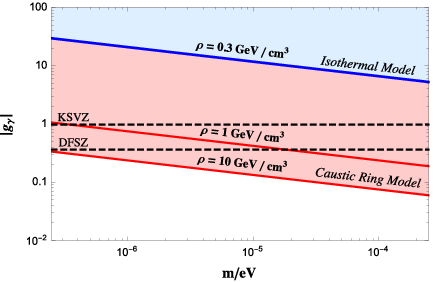
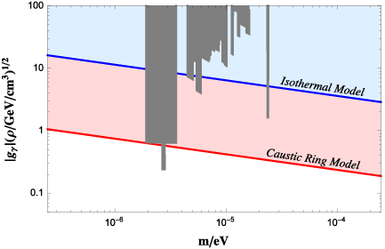
The echo method appears an attractive approach to axion dark matter detection because it uses relatively old technology and because it is applicable over a wide range of axion masses. The method works better in the caustic ring model than in the isothermal model for three reasons: 1) the density is higher, 2) the echo has less spread in frequency, and 3) the echo has less spread in physical space. Higher density helps the cavity method equally. Fig. 2 shows the sensitivity of the echo method to as well as the published limits obtained by searches using the cavity method. The small spread in frequency of a signal from a cold flow, such as the Big Flow of the caustic ring model, also helps somewhat the cavity method. Ref. Hires describes a high resolution analysis of ADMX data and shows that an improvement by a factor of order 2 in is obtained in case of a cold flow of velocity dispersion less than 10 m/s. The improvements in sensitivity of the cavity method in case of cold flows are not included in the published bounds shown in Fig. 2.
We thank Richard Bradley, Fritz Caspers, Guido Mueller, Neil Sullivan, David Tanner, Qiaoli Yang and Konstantin Zioutas for useful discussions. This research was supported in part by the U.S. Department of Energy under grant DE-SC0010296, by the Chilean Commission on Research, Science and Technology (CONICYT) under grant 78180100 (Becas Chile, Postdoctorado), and by the Heising-Simons Foundation under grant No. 2015-109.
References
- (1) Reviews include: Particle Dark Matter edited by Gianfranco Bertone, Cambridge University Press 2010; E.W. Kolb and M. Turner, The Early Universe, Addison Wesley 1990.
- (2) R. D. Peccei and H. Quinn, Phys. Rev. Lett. 38 (1977) 1440 and Phys.Rev. D16 (1977) 1791; S. Weinberg, Phys. Rev. Lett. 40 (1978) 223; F. Wilczek, Phys. Rev. Lett. 40 (1978) 279.
- (3) J. Kim, Phys. Rev. Lett. 43 (1979) 103; M. A. Shifman, A. I. Vainshtein and V. I. Zakharov, Nucl. Phys. B166 (1980) 493.
- (4) M. Dine, W. Fischler and M. Srednicki, Phys. Lett. B104 (1981) 199; A. Zhitnitskii, Sov. J. Nucl. 31 (1980) 260.
- (5) G. Raffelt, Lect. Notes Phys. D79 (2008) 51.
- (6) J. Preskill, M. Wise and F. Wilczek, Phys. Lett. B120 (1983) 127; L. Abbott and P. Sikivie, Phys. Lett. B120 (1983) 133; M. Dine and W. Fischler, Phys. Lett. B120 (1983) 137.
- (7) J. Ipser and P. Sikivie, Phys. Rev. Lett. 50 (1983) 925.
- (8) P. Sikivie, Lect. Notes Phys. 741 (2008) 19. D.J.E. Marsh, Phys. Rep. 643 (2016) 1.
- (9) H. Baer, V. Barger and D. Sengupta, Phys. Lett. B790 (2019) 58, and references therein.
- (10) P. Svrcek and E. Witten, JHEP 0606 (2006) 051.
- (11) P. Arias et al., JCAP 1206 (2012) 013, and references therein.
- (12) P. Sikivie, Phys. Rev. Lett. 51 (1983) 1415 and Phys. Rev. D32 (1985) 2988.
- (13) S.J. Asztalos et al., Phys. Rev. Lett. 104 (2010) 041301; N. Du et al., Phys. Rev. Lett. 120 (2018) 151301; B.M. Brubaker et al., Phys. Rev. Lett. 118 (2017) 061302; S. Youn, Int. J. Mod. Phys. Conf. Ser. 43 (2016) 1660193; B.T. McAllister et al., Phys. Dark Univ. 18 (2017) 67.
- (14) P. Sikivie, D.B. Tanner and Y. Wang, Phys. Rev. D50 (1994) 4744; G. Rybka and A. Wagner, Phys. Rev. D91 (2015) 011701.
- (15) A. Caldwell et al., Phys. Rev. Lett. 118 (2017) 091801.
- (16) P. Graham and S. Rajendran, Phys. Rev. D88 (2013) 035023; D. Budker et al., Phys. Rev. X 4 (2014) 021030; P. Graham et al., Phys. Rev. D97 (2018) 055006.
- (17) R. Barbieri et al., Phys. Dark Univ. 15 (2017) 135.
- (18) P. Sikivie, N. Sullivan and D.B. Tanner, Phys. Rev. Lett. 112 (2014) 131301; Y. Kahn, B. Safdi and J. Thaler, Phys. Rev. Lett. 117 (2016) 141801; B.T. McAllister, S.R. Parker and M.E. Tobar, Phys. Rev. D94 (2016) 042001; N. Crisosto et al., Springer Proc. Phys. 211 (2018) 127; J.L. Ouellet et al., Phys. Rev. Lett. 122 (2019) 121802.
- (19) P. Sikivie, Phys. Rev. Lett. 113 (2014) 201301; C. Braggio et al., Sci. Rep. 7 (2017) 15168; V.V. Flambaum et al., J. Mod. Phys. A33 (2018) 1844030.
- (20) Y. Inoue et al., Phys. Lett. B668 (2008) 93; V. Anastassopoulos et al., Nature Physics 13 (2017) 584; E. Armengaud et al., JINST 9 (2014) T05002.
- (21) F. Avignone et al., Phys. Rev. Lett. 81 (1998) 5068.
- (22) S. Dimopoulos, G.D. Starkman and B.W. Lynn, Phys. Lett. B168 (1986) 145; D.S. Akerib et al., Phys. Rev. Lett. 118 (2017) 261301, and references therein.
- (23) K. van Bibber et al., Phys. Rev. Lett. 59 (1987) 759; K. Ehret et al., Phys. Lett. B689 (2010) 149, and references therein; R. Ballou et al., Phys. Rev. D92 (2015) 092002; F. Hoogeveen and T. Ziegenhagen, Nucl. Phys. B358 (1991) 3; G. Mueller, P. Sikivie, D. Tanner and K. van Bibber, Phys. Rev. Lett. D80 (2009) 072004.
- (24) Y.V. Stadnik and V.V. Flambaum, Phys. Rev. D89 (2014) 043522.
- (25) I.I. Tkachev, JETP Lett. 101 (2015) 1; A. Arza, Eur. Phys. J. C79 (2019) 250; A. Caputo et al., JCAP 1903 (2019) 27; A. Caputo, C. Peña Garay and S.J. Witte, Phys. Rev. D98 (2018) 083024 and Erratum: Phys. Rev. D99 (2019) 089901.
- (26) See Supplemental Material at [URL …] for a derivation of these results.
- (27) M.S. Turner, Phys. Rev. D33 (1986) 889.
- (28) L. Duffy and P. Sikivie, Phys. Rev. D78 (2008) 063508.
- (29) N. Banik and P. Sikivie, Phys. Rev. D93 (2016) 103509.
- (30) S. Chakrabarty, A. Gonzales, Y. Han and P. Sikivie, to be published.
- (31) https://science.nrao.edu/facilities/gbt/proposing/GBTpg.pdf .
- (32) L. Duffy et al., Phys. Rev. Lett. 95 (2005) 091304 and Phys. Rev. D74 (2006) 012006.