跳到论文正文
W Papers独立论文阅读器 arXiv:1901.11510 论文正文 计算阅读时间 · 0%
引用这篇论文根据当前论文元数据生成,正式投稿前建议核对。


License: arXiv.org perpetual non-exclusive license
arXiv:1901.11510v2 [hep-ph] 10 May 2019

Decomposition of Feynman Integrals on the Maximal Cut by Intersection Numbers

Hjalte Frellesvig Affiliation: Dipartimento di Fisica e Astronomia, Università di Padova, Via Marzolo 8, 35131 Padova, Italy Affiliation: INFN, Sezione di Padova, Via Marzolo 8, 35131 Padova, Italy Email: hjalte.frellesvig@pd.infn.it    Federico Gasparotto Affiliation: Dipartimento di Fisica e Astronomia, Università di Padova, Via Marzolo 8, 35131 Padova, Italy Affiliation: INFN, Sezione di Padova, Via Marzolo 8, 35131 Padova, Italy Email: federico.gasparotto@pd.infn.it    Stefano Laporta Affiliation: Dipartimento di Fisica e Astronomia, Università di Padova, Via Marzolo 8, 35131 Padova, Italy Affiliation: INFN, Sezione di Padova, Via Marzolo 8, 35131 Padova, Italy Email: stefano.laporta@pd.infn.it    Manoj K. Mandal Affiliation: Dipartimento di Fisica e Astronomia, Università di Padova, Via Marzolo 8, 35131 Padova, Italy Affiliation: INFN, Sezione di Padova, Via Marzolo 8, 35131 Padova, Italy Email: manojkumar.mandal@pd.infn.it    Pierpaolo Mastrolia Affiliation: Dipartimento di Fisica e Astronomia, Università di Padova, Via Marzolo 8, 35131 Padova, Italy Affiliation: INFN, Sezione di Padova, Via Marzolo 8, 35131 Padova, Italy Email: pierpaolo.mastrolia@pd.infn.it    Luca Mattiazzi Affiliation: Dipartimento di Fisica e Astronomia, Università di Padova, Via Marzolo 8, 35131 Padova, Italy Affiliation: INFN, Sezione di Padova, Via Marzolo 8, 35131 Padova, Italy Email: luca.mattiazzi@pd.infn.it    Sebastian Mizera Affiliation: Perimeter Institute for Theoretical Physics, Waterloo, ON N2L 2Y5, Canada Affiliation: Department of Physics & Astronomy, University of Waterloo, Waterloo, ON N2L 3G1, Canada Email: smizera@pitp.ca
Abstract

We elaborate on the recent idea of a direct decomposition of Feynman integrals onto a basis of master integrals on maximal cuts using intersection numbers. We begin by showing an application of the method to the derivation of contiguity relations for special functions, such as the Euler beta function, the Gauss F12{}_{2}F_{1} hypergeometric function, and the Appell F1F_{1} function. Then, we apply the new method to decompose Feynman integrals whose maximal cuts admit 1-form integral representations, including examples that have from two to an arbitrary number of loops, and/or from zero to an arbitrary number of legs. Direct constructions of differential equations and dimensional recurrence relations for Feynman integrals are also discussed. We present two novel approaches to decomposition-by-intersections in cases where the maximal cuts admit a 2-form integral representation, with a view towards the extension of the formalism to nn-form representations. The decomposition formulae computed through the use of intersection numbers are directly verified to agree with the ones obtained using integration-by-parts identities.

1 Introduction

The highly interactive nature of elementary-particle dynamics is an extremely complex problem to describe. Feynman diagrams play a fundamental role by encoding how, within the perturbative approach to quantum field theory, complex scattering reactions may arise from the multiple interactions among simpler network components, representing either external or internal particles. For each scattering process, the sum of all diagrams gives the so called scattering amplitude, a complex function of external kinematics (and internal quantum numbers) whose absolute squared value determines the quantum-mechanical density of probability for that reaction to happen.

The shape of the diagrams informs directly about the complexity level of the process they describe, which increases with the number of interacting external particles, the number of interaction vertices, and with the number of loops. In general, Feynman diagrams represent functions of kinematic invariants formed by the external momenta and by the masses of the particles. While scattering amplitudes associated to tree-level graphs can be written in terms of rational functions, those coming from multi-loop graphs are usually decomposed into special functions admitting multifold integral representations.

Feynman integrals in dimensional regularization are known to be not mutually independent. A novel way to access their algebraic structure has been recently unveiled by some of us, who showed that relations for multi-loop Feynman integrals are controlled by intersection numbers Mastrolia:2018uzb.

The by-now standard evaluation techniques of Feynman integrals exploit the loop-momentum shift invariance to establish integration-by-parts (IBP) relations Chetyrkin:1981qh among integrals whose integrands are built out of products of the same set of denominators (and scalar products), but raised to different powers. IBP identities have been playing a crucial role in the calculation of multi-loop integrals, because they yield the identification of a minimal set of elements, dubbed master integrals (MIs), which can be used as a basis for the decomposition of multi-loop amplitudes. At the same time, IBP-decomposition algorithms can be applied to special integrands, built by acting on the master integrand with differential operators (w.r.t. kinematic invariants), or by multiplying their numerators by polynomials which modify their dimensions, or by considering arbitrary denominator powers, respectively turning the decomposition formulas into differential equations Barucchi:1973zm; KOTIKOV1991158; KOTIKOV1991123; Bern:1993kr; Remiddi:1997ny; Gehrmann:1999as; Henn:2013pwa; Henn:2014qga, dimensional recurrence relations Tarasov:1996br; Lee:2009dh, and finite difference equations Laporta:2001dd; Laporta:2003jz obeyed by MIs. Solving them amounts to the actual determination of the MIs themselves, as an alternative to the use of direct integration techniques.

The derivation of the IBP-decomposition formulas requires the solution of a large system of linear relations, generated by imposing that integrals of total derivatives vanish on the integration boundary Laporta:2001dd, see also smirnov2005evaluating; Grozin:2011mt; Zhang:2016kfo; Kotikov:2018wxe. For multi-loop multi-scale scattering amplitudes, solving the system of IBP relations may however represent a formidable task, whose accomplishment has been motivating important refinements of the system-solving strategies vonManteuffel:2014ixa; Peraro:2016wsq; Boehm:2018fpv; Kosower:2018obg; Liu:2018dmc; Kardos:2018uzy; Chawdhry:2018awn; vonManteuffel:2012np; Lee:2012cn; Smirnov:2008iw; Maierhoefer:2017hyi; Georgoudis:2016wff; Maierhofer:2018gpa; Smirnov:2019qkx. Together with novel algorithms for simplifying the solution of systems of differential equations Henn:2013pwa, which triggered further studies Argeri:2014qva; Lee:2014ioa; Gehrmann:2014bfa; Gituliar:2017vzm; Lee:2017oca; Adams:2018yfj, the calculations of several multi-scale, multi-loop, multi-particle amplitudes became feasible Laporta:2017okg; Anastasiou:2015ema; Bonciani:2015eua; Gehrmann:2015dua; Bonetti:2017ovy; Borowka:2016ypz; Baglio:2018lrj; Lindert:2017pky; Jones:2018hbb; Maltoni:2018zvp; Gehrmann:2015bfy; Badger:2017jhb; Abreu:2018jgq; Abreu:2018zmy; Chicherin:2018yne; Abreu:2018aqd; Badger:2018enw; Chicherin:2019xeg; Abreu:2019rpt.

The most recent developments in the research of mathematical methods for the evaluation of Feynman integrals have been benefiting from a special representation known as Baikov representation Baikov:1996iu, where instead of the components of the loop momenta, the propagators themselves supplemented by independent scalar products between external and internal momenta, are the integration variables. This change of variables introduces a Jacobian equal to the Gram determinant of the scalar products formed by both types of momenta, referred to as the Baikov polynomial. The Baikov polynomial fully characterizes the space on which the integrals are defined, and in particular the number of MIs can be inferred from the number of its critical points Lee:2013hzt, see also Marcolli:2008vr; marcolli2010feynman; Bitoun:2017nre. IBP identities may relate integrals corresponding to a given graph to integrals that correspond to its sub-graphs. We may consider these two sets of integrals, respectively, as to the homogeneous and the non-homogenous terms of the IBP relations. The homogeneous terms of IBP identies can be detected by maximal cuts, since the multiple cut-conditions annihilate the terms corresponding to subdiagrams Larsen:2015ped; Bosma:2017hrk; Frellesvig:2017aai; Zeng:2017ipr; Bosma:2017ens; Harley:2017qut; Boehm:2018fpv. By the same arguments, maximal cuts of MIs correspond to the homogeneous solutions of dimensional recurrence relations and of the differential equations, which, in general, are non-homogeneous equations Lee:2012te; Remiddi:2016gno; Primo:2016ebd; Primo:2017ipr. Similar ideas were introduced Anastasiou:2002yz and lead to relation between multi-loop integrals and phase-space integrals, known as reverse unitarity. The homogeneous solutions play an important role in the construction of canonical systems of differential equation for MIs Henn:2013pwa, as it was observed in Remiddi:2016gno; Primo:2016ebd; Primo:2017ipr, generalizing the role of Magnus exponential matrix Argeri:2014qva to the case of elliptic equations.

The number of MIs for a given integral family, the order of the differential equations they obey, and the classification of the homogeneous solutions according to the independent components of the integration domain, revealed a natural correspondence between the MIs and the geometric properties of the integration domain Laporta:2004rb; Remiddi:2016gno; Primo:2016ebd; Primo:2017ipr; Bosma:2017ens; vonManteuffel:2017hms; Frellesvig:2017aai; Harley:2017qut; Adams:2018kez, easily accessed within Baikov representation.

Let us imagine, for a moment, that the objective of a calculation is simply the decomposition in terms of master integrals of just one multi-loop Feynman integral. The IBP reduction algorithm can be seen as a collective integral decomposition. The computational machinery does not act on individual integrals, one at a time, but it is based on the solution of systems of equations where the wanted integral appears related, within linear relations, to many additional integrals. Its decomposition is then achieved together with the decomposition of other integrals – even if the latter might not be of interests, for instance. The IBP decomposition, although very effective, is computationally expensive.

The new computational strategy proposed in ref. Mastrolia:2018uzb offers a change of perspective: it targets the direct decomposition of individual integrals in terms of master integrals, bypassing the system solving procedure characterizing the integration-by-parts reduction.

This task can be achieved by applying to Feynman integrals concepts and computational tools borrowed from the intersection theory of differential forms cho1995; matsumoto1998; Mizera:2017rqa. It is a recent branch of algebraic geometry and topology, which was developed to study the Aomoto–Gel’fand hypergeometric functions aomoto2011theory. This class of functions has two important properties: their integrands are multivalued, and vanish at the boundaries of the integration domain - exactly like Feynman integrals in dimensional regularization. Baikov representation makes these properties manifest, and allows to establish an explicit correspondence between Feynman integrals and the functions which can be studied via intersection theory. In particular, any Feynman integral is cast as a nn-form integral, characterized by three basic elements: the integration contour, part of its integrand given by a multivalued function (associated to the Baikov polynomial), and a differential form (corresponding to the genuine product of denominators times the integration measure).

In general, two integrals can give the same result if: they have the same integration domain, but their integrands differ by a term whose primitive vanishes on the integration boundaries; and/or they have the same integrand, but their integration domains differ by a contour on which the primitive vanish anyhow. Therefore each integral is actually a pairing of representatives of two equivalence classes: characterized by the integration variety (homology class) or by the integrand (cohomology class). Intersection theory allows for a derivation of relations among integrals belonging to those equivalence classes, which in the case of hypergeometric functions correspond to Gauss’ contiguity relations. In ref. Mastrolia:2018uzb, the concepts of intersection theory were applied to Feynman integrals in order to show that it is possible: i) to identify a basis of master integrals; ii) to decompose any individual integral in the chosen basis simply by a projection technique; iii) to derive differential equations for master integrals. The so-called intersection number of differential forms cho1995; matsumoto1998 constitutes the crucial novel operation that allows to implement the notion of scalar products between differential forms, which ultimately determine the coefficients of the integral decomposition. In this way, the problem of reducing a given Feynman integral in terms of master integrals can be solved by projections: any integral can be decomposed just like an arbitrary vector can be projected onto a chosen basis of a vector space. This analysis was performed by considering integrals on maximal cuts admitting 1-form representations Mastrolia:2018uzb.

In this work, we elaborate on the decomposition-by-intersection of Feynman integrals onto a basis of master integrals, and we systematically apply it to an extensive list of cases, in order to show its advantages.

We begin by recalling basics of intersection theory for hypergeometric functions, and show their correspondence to the Baikov representation, both in the standard formulation Baikov:1996iu and in the Loop-by-Loop version Frellesvig:2017aai. We then define how intersection theory allows to determine the dimension of the integral space, and discuss different options for the choice of the integral bases. Afterwards, we introduce the intersections numbers and give the master decomposition formula for the direct evaluation of the coefficients of the reduction in terms of basis integrals. This formula can be also applied to derive differential equations and dimensional recurrence relations for generic basis integrals.

Before addressing Feynman calculus, we consider the derivation of contiguity relations for special functions, such as the Euler β\beta function, the Gauss F12{}_{2}F_{1} hypergeometric function, and the Appell F1F_{1} function, which belong to the more general class of Lauricella functions. Then, we apply the new method to decompose Feynman integrals whose maximal cuts admit 1-form integral representations, including examples that have from two to an arbitrary number of loops, and/or from zero to an arbitrary number of legs. The 1-form integral representations accounts for multi-loop integrals (on maximal cuts) which have either one irreducible scalar product (ISP), or that have multiple ISPs but can be expressed as a one-fold integral using the Loop-by-Loop approach,

In a few instructive cases, we show the direct constructions of differential equations and dimensional recurrence relations for master integrals, and discuss how the different choice of the basis may impact of the form of the result. Special emphasis is given to basis of monomial forms and to basis of dlog forms, in particular showing how, the latter obey a canonical systems of differential equations.

As stressed, the main part of this work deals with the application of intersection theory to 1-forms. The complete decomposition of multi-loop Feynman integrals in terms of master integrals (not just the ones belonging to maximal-cut diagrams, but to the complete chain of sub-diagrams, which would correspond to a smaller number of cuts) requires the application of the intersection theory for nn-forms. In the literature, the case of intersection numbers of dlog nn-forms has been understood matsumoto1998; Mizera:2017rqa, but Feynman integrals belong to the wider class of generic rational nn-forms.

As additional main results of this manuscript, we present two novel approaches to decomposition-by-intersections in cases where the maximal cuts admit a 2-form integral representation. They are important new development both for physical and mathematical research areas, as they represent the first step towards the extension of the formalism to generic nn-form representations. Owing to the results of the research presented in this work, we are confident that this objective is within reach.

The decomposition formulae computed through the use of intersection numbers for 1- and 2-forms are directly verified to agree with the ones obtained using integration-by-parts identities on the maximal cut. As reported in the examples discussed later, we employed several codes for checking our results, and when available, we compared them with the literature. Let us finally observe that, in a few cases, the number of master integrals (on the maximal cuts) found by means of intersection theory is smaller than the one found by applying the IBP-decomposition to the interested integral families: the mismatch has been mitigated by finding the additional, missing relations at the cost of applying the IBP-reduction to integrals families with a larger number of denominators.

The results presented in this paper demonstrate that a fascinating property of Feynman integrals has been found, which opens a completely new path to access their algebraic structures. Together with the idea of dimensional regularization, its main application to streamlining reductions unto master integrals, is expected to yield significant computational advantages for the evaluation of high-multiplicity scattering amplitudes at higher orders in perturbation theory.

The paper is organized as follows. In Sec. 2 we introduce the basics of hypergeometric integrals, and their description in terms of (co)homology and intersection theory. Significantly this section introduces the master decomposition formula eq. (14). Then follows Sec. 3 in which we discuss Feynman integrals, the Baikov representations, unitarity cuts, and the connection to intersection theory. The section also discusses relations between Feynman integrals such as reductions unto master integrals, differential equations, and dimensional recurrence.

In Sec. 4 we discuss certain specific mathematical functions to which our theory is applicable, which serve as our first examples. These are the β\beta-function, the F12{}_{2}F_{1}, the Appell F1F_{1}, and the Lauricella FDF_{D}. The next two sections, Secs. 5 and 6, contain our first examples of the use of the theory to Feynman integrals: a four-loop vacuum integral, and a three-loop two-point function respectively. These two integrals are put in a one-form representation by the standard Baikov parametrization. In Sec. 7 we discuss the sunrise integral in a massless and a massive version. These integrals can be put into a one-form representation by the Loop-by-Loop version of Baikov parametrization, where the standard version of Baikov representation would have left them as a two-fold integrals. In Sec. 8 we return to the non-planar triangle of ref. Mastrolia:2018uzb, and show how to use our method to deal with doubled propagators. Then in Sec. 9 follows an example of a planar triangle diagram with only one master integral, showing the intersection approach alongside a traditional cut-based extraction. Sec. 10 discusses a certain planar diagram, that is of interest due to peculiar properties of the Baikov polynomial, something that in the past has led to ambiguities in the counting of master integrals in that sector. Secs. 11 and 12 discuss two double-box integrals, with and without an internal mass. The massive case is of interest as this is our first example in which the intersection theory on the maximal cut, detects a relation that is not usually found by IBP identities. The next two sections applies the theory to some cases of physical interest, namely Bhabha scattering in Sec. 13, and associated Higgs production (H+jH{+}j and H​HHH) in Sec. 14. These two cases are at the edge of what is possible to fully reduce with traditional IBP methods. Then follows Sec. 15 on the celebrated penta-box in a planar and a non-planar version and Sec. 16 about its generalizations to cases with massive legs, and significantly to cases with more legs, including an nn-leg example. In Sec. 17 we look some high-loop integrals (planar and non-planar) that contribute to H+jH{+}j production, and we show several nn-loop generalizations thereof (that we denote “rocket diagrams”), including their reductions unto master integrals, and their differential equations.

The following two sections contain discussions on the extension of the one-form algorithm described in this paper, to higher forms. Sec. 18 discusses one approach that consists of iterating the one-form algorithm combined with direct integration. Sec. 19 discusses another genuinely multivariate approach in which the intersection numbers are computed using intersecting hyperplanes. Finally Sec. 20 contains our conclusions and discussion. The paper ends with two appendices. First App. A in which we discuss the relation between the number of critical points and the number of master integrals. In particular we calculate the number of critical points with both the standard and the Loop-by-Loop approaches to Baikov parametrization on the maximal cut, and we discuss in detail the cases in which the two numbers thereby obtained are in disagreement. Then follows App. B in which we we use the iterated one-form algorithm to derive expressions for the integrand in the Loop-by-Loop approach when the ISPs that get integrated out are present.

2 Basics of Hypergeometric Integrals

In this section we review a few concepts from the theory of hypergeometric functions and Feynman integrals that serve as a basis for the remainder of the paper.

Consider an integral II over the variables 𝐳=(z1,z2,…,zm){\bf z}=(z_{1},z_{2},\ldots,z_{m}) of the general form:

I=∫𝒞u⁡(𝐳)​φ​(𝐳),I=\int_{\mathcal{C}}u(\mathbf{z})\,\varphi(\mathbf{z}), (1)

where u⁡(𝐳)u(\mathbf{z}) is a multi-valued function and φ⁡(𝐳)=φ^​(𝐳)​dm​𝐳\varphi(\mathbf{z})=\hat{\varphi}(\mathbf{z})d^{m}\mathbf{z} is a differential mm-form. We assume that u⁡(𝐳)u(\mathbf{z}) vanishes on the boundaries of 𝒞\mathcal{C}, u⁡(∂𝒞)=0u(\partial{\cal C})=0, so that, upon integration no surface-term is leftover. For example, choosing

u⁡(z)=za​(z−1)b,φ⁡(z)=d​zz⁡(z−1),𝒞=[0,1]u(z)=z^{a}(z-1)^{b},\qquad\varphi(z)=\frac{dz}{z(z-1)},\qquad\mathcal{C}=[0,1] (2)

gives the Euler beta function B⁡(a,b)B(a,b) for Re​(a),Re​(b)>0\text{Re}(a),\text{Re}(b)>0. More generally, integrals of the type (1) are called Aomoto–Gel’fand hypergeometric functions aomoto1977structure; Gelfand, or simply hypergeometric functions.

As with any integral, there could exist many forms φ\varphi that integrate to give the same result II. Let us consider the total derivative of uu times any (m−1)(m{-}1)-differential form ξ\xi:

∫𝒞d⁡(u​ξ)=0.\int_{\mathcal{C}}d\left(u\,\xi\right)=0. (3)

By Stokes’ theorem, the result is zero due to our choice of the integration domain 𝒞\mathcal{C}. Let us manipulate the above integral so that it is of the form (1):

0=∫𝒞d⁡(u​ξ)=∫𝒞(𝑑u∧ξ+u​𝑑ξ)=∫𝒞u⁡(d​uu∧+d)​ξ≡∫𝒞u​∇ωξ.0=\int_{\mathcal{C}}d\left(u\,\xi\right)=\int_{\mathcal{C}}\left(du\wedge\xi+u\,d\xi\right)=\int_{\mathcal{C}}u\left(\frac{du}{u}\wedge+\,d\right)\xi\equiv\int_{\mathcal{C}}u\,\nabla_{\omega}\xi. (4)

In the final equality we defined a connection ∇ω\nabla_{\omega}, which differs from the usual derivative by the one-form ω\omega:

∇ω≡d+ω∧,whereω≡d​log⁡u.\nabla_{\omega}\equiv d+\omega\wedge,\qquad\text{where}\qquad\omega\equiv d\log u. (5)

Since the above expression integrates to zero, we have

∫𝒞u​φ=∫𝒞u⁡(φ+∇ωξ).\int_{\mathcal{C}}u\,\varphi=\int_{\mathcal{C}}u\left(\varphi+\nabla_{\omega}\xi\right). (6)

Hence φ\varphi and φ+∇ωξ\varphi+\nabla_{\omega}\xi carry the same information and we can talk about equivalence (cohomology) classes ⟨φ|ω{{}_{\omega}}\langle\varphi| of forms that integrate to the same result:

⟨φ|:φ∼φ+∇ωξ.ω{{}_{\omega}}\langle\varphi|:\;\varphi\sim\varphi+\nabla_{\omega}\xi. (7)

In other words, whenever two forms are equal to each other up to integration-by-parts identities, they belong to the same equivalence class. This class is called a twisted cocycle. The word twisted refers to the fact that the usual derivative operator dd is replaced by the covariant derivative ∇ω\nabla_{\omega} given in (5), as a consequence of the presence of the multi-valued function uu in the hypergeometric integral. We often refer to any representative of the class (7) as twisted cocycle, as well as drop the subscript ω when it is clear from the context.11 1 For completeness, let us mention that, similarly, there are equivalence (homology) classes of integration domains 𝒞\mathcal{C} that give the same result for the integral (1), called twisted cycles |𝒞]ω|\mathcal{C}]_{\omega}, though we do not make use of this fact in the current manuscript. A remarkable observation is that we can pair up ⟨φ|\langle\varphi| and |𝒞]|\mathcal{C}] to obtain the integral from (1), which we denote by

⟨φ|𝒞]≡∫𝒞uφ.\langle\varphi|\mathcal{C}]\equiv\int_{\mathcal{C}}u\,\varphi. (8)

This integral representation, as a bilinear in ⟨φ|\langle\varphi| and |𝒞]|\mathcal{C}], is suitable for establishing linear relations between hypergeometric functions. In fact, let us assume that the number of linearly-independent twisted cocycles is ν\nu, and indicate an arbitrary basis of forms,

⟨e1|,⟨e2|,⋯,⟨eν|.\langle e_{1}|,\quad\langle e_{2}|,\quad\cdots,\quad\langle e_{\nu}|. (9)

A basis decomposition is achieved by expressing an arbitrary twisted cocycle, say ⟨φ|\langle\varphi|, as a linear combination of the above ones. This goal be achieved as follows. Introduce a dual (and auxiliary) space of twisted cocycles, whose basis is denoted by |hi⟩|h_{i}\rangle for i=1,2,…,νi=1,2,\ldots,\nu, and consider the matrix 𝐂{\bf C}, whose entries are the pairing ⟨ei|hj⟩\langle e_{i}|h_{j}\rangle,

𝐂i​j=⟨ei|hj⟩fori,j=1,2,…,ν.\displaystyle\mathbf{C}_{ij}=\langle e_{i}|h_{j}\rangle\qquad\text{for}\qquad i,j=1,2,\ldots,\nu\ . (10)

This pairing is called the intersection number of ⟨ei|\langle e_{i}| and |hj⟩|h_{j}\rangle. We then construct the (ν+1)×(ν+1)(\nu{+}1)\times(\nu{+}1) matrix 𝐌{\bf M}, defined as,

𝐌=(⟨φ|ψ⟩⟨φ|h1⟩⟨φ|h2⟩…⟨φ|hν⟩⟨e1|ψ⟩⟨e1|h1⟩⟨e1|h2⟩…⟨e1|hν⟩⟨e2|ψ⟩⟨e2|h1⟩⟨e2|h2⟩…⟨e2|hν⟩⋮⋮⋮⋱⋮⟨eν|ψ⟩⟨eν|h1⟩⟨eν|h2⟩…⟨eν|hν⟩)≡(⟨φ|ψ⟩𝐀⊺𝐁𝐂).\mathbf{M}=\left(\begin{array}[]{ccccc}\langle\varphi|\psi\rangle&\langle\varphi|h_{1}\rangle&\langle\varphi|h_{2}\rangle&\ldots&\langle\varphi|h_{\nu}\rangle\\ \langle e_{1}|\psi\rangle&\langle e_{1}|h_{1}\rangle&\langle e_{1}|h_{2}\rangle&\ldots&\langle e_{1}|h_{\nu}\rangle\\ \langle e_{2}|\psi\rangle&\langle e_{2}|h_{1}\rangle&\langle e_{2}|h_{2}\rangle&\ldots&\langle e_{2}|h_{\nu}\rangle\\ \vdots&\vdots&\vdots&\ddots&\vdots\\ \langle e_{\nu}|\psi\rangle&\langle e_{\nu}|h_{1}\rangle&\langle e_{\nu}|h_{2}\rangle&\ldots&\langle e_{\nu}|h_{\nu}\rangle\end{array}\right)\equiv\left(\begin{array}[]{cc}\langle\varphi|\psi\rangle&\mathbf{A}^{\intercal}\\ \mathbf{B}&\mathbf{C}\end{array}\right). (11)

The columns of the matrix 𝐌\mathbf{M} are labelled by |ψ⟩,|h1⟩,|h2⟩,…,|hν⟩|\psi\rangle,|h_{1}\rangle,|h_{2}\rangle,\ldots,|h_{\nu}\rangle for an arbitrary |ψ⟩|\psi\rangle, while the rows are labelled by ⟨φ|,⟨e1|,⟨e2|,…,⟨eν|\langle\varphi|,\langle e_{1}|,\langle e_{2}|,\ldots,\langle e_{\nu}|. Each entry is given by a pairing (bilinear) of the corresponding row and column. In the second equality, we expose the structure of 𝐌\mathbf{M} as a ν×ν\nu\times\nu submatrix 𝐂\mathbf{C}, a column vector 𝐁\mathbf{B} and a row vector 𝐀⊺\mathbf{A}^{\intercal}, respectively with elements 𝐁i=⟨ei|ψ⟩\mathbf{B}_{i}=\langle e_{i}|\psi\rangle and 𝐀i=⟨φ|hi⟩\mathbf{A}_{i}=\langle\varphi|h_{i}\rangle (for i=1,2,…,νi=1,2,\ldots,\nu).

The fact that the ν+1\nu{+}1 cocycles labelling the rows and columns are necessarily linearly dependent (since the basis is ν\nu-dimensional) and that each entry of 𝐌\mathbf{M} is a bilinear, implies that the determinant of this matrix vanishes. Using the well-known identity for the determinant of a block matrix, we find:

det⁡𝐌=det⁡𝐂⁡(⟨φ|ψ⟩−𝐀⊺​𝐂−1​𝐁)=0.\det\mathbf{M}=\det\mathbf{C}\,\bigg(\langle\varphi|\psi\rangle-\mathbf{A}^{\intercal}\,\mathbf{C}^{-1}\,\mathbf{B}\bigg)=0. (12)

In addition, det⁡𝐂\det\mathbf{C} cannot be zero (by definition), since it is formed from bilinears between two bases. Therefore we conclude that:

⟨φ|ψ⟩\displaystyle\langle\varphi|\psi\rangle =𝐀⊺​𝐂−1​𝐁\displaystyle=\mathbf{A}^{\intercal}\,\mathbf{C}^{-1}\,\mathbf{B}
=∑i,j=1ν⟨φ|hj⟩​(𝐂−1)j​i​⟨ei|ψ⟩.\displaystyle=\sum_{i,j=1}^{\nu}\langle\varphi|h_{j}\rangle\,(\mathbf{C}^{-1})_{ji}\,\langle e_{i}|\psi\rangle. (13)

Given the arbitrariness of |ψ⟩|\psi\rangle, we obtain the master decomposition formula

⟨φ|=∑i,j=1ν⟨φ|hj⟩​(𝐂−1)j​i​⟨ei|,\langle\varphi|=\sum_{i,j=1}^{\nu}\langle\varphi|h_{j}\rangle\,\left(\mathbf{C}^{-1}\right)_{ji}\,\langle e_{i}|, (14)

which provides an explicit way of projecting ⟨φ|\langle\varphi| onto a basis of ⟨ei|\langle e_{i}|. Following Mastrolia:2018uzb, in this paper we use (14) to perform the decomposition of Feynman integrals in terms of master integrals, on the maximal cut. For example, by contracting both sides with the twisted cycle |𝒞]|\mathcal{C}] (which boils down to multiplying by uu and integrating over 𝒞\mathcal{C}), we have a linear identity between integrals:

∫𝒞u​φ=∑i,j=1ν⟨φ|hj⟩​(𝐂−1)j​i​∫𝒞u​ei.\int_{\mathcal{C}}u\,\varphi=\sum_{i,j=1}^{\nu}\langle\varphi|h_{j}\rangle\,\left(\mathbf{C}^{-1}\right)_{ji}\int_{\mathcal{C}}u\,e_{i}. (15)

Similarly, the same idea can be used to derive linear system of differential equations satisfied by the basis integrals ⟨ei|𝒞]\langle e_{i}|\mathcal{C}] in some external variable xx. It is enough to notice that

∂x⟨ei|𝒞]=∂x∫𝒞uei=∫𝒞u(∂x+σ∧)ei=⟨(∂x+σ∧)ei|𝒞],\partial_{x}\,\langle e_{i}|{\cal C}]=\partial_{x}\int_{\cal C}u\,e_{i}=\int_{\cal C}u\,(\partial_{x}+\sigma\wedge)e_{i}=\langle(\partial_{x}+\sigma\wedge)e_{i}|\mathcal{C}], (16)

where σ≡∂xlog⁡(u)\sigma\equiv\partial_{x}\log(u). Let us remark that even if 𝒞{\cal C} depends on xx, the differential operator ∂x\partial_{x} commutes with the integral sign, due to the vanishing of uu on the boundary of 𝒞\mathcal{C}. Therefore, the problem reduces to projecting ⟨(∂x+σ∧)ei|\langle(\partial_{x}+\sigma\wedge)e_{i}| on the right-hand side back onto a basis using (14).

One should think of ⟨ei|\langle e_{i}| and |hj⟩|h_{j}\rangle as parameterizing a vector space of inequivalent integrands of a hypergeometric function. In this sense 𝐂\mathbf{C} provides a metric on this space. Naturally, the prescription (14) is only useful if computing invariants of the type ⟨φL|φR⟩\langle\varphi_{L}|\varphi_{R}\rangle is efficient. We argue that this is the case. It turns out that the dual space of twisted cocycles has a straightforward interpretation as the equivalence classes:

|φ⟩ω:φ∼φ+∇−ωξ,|\varphi\rangle_{\omega}:\;\varphi\sim\varphi+\nabla_{-\omega}\xi, (17)

where the only difference to (7) is the use of the connection ∇−ω≡d−ω∧\nabla_{-\omega}\equiv d-\omega\wedge instead of ∇ω\nabla_{\omega}. The resulting bilinear:

⟨φL|φR⟩ω\langle\varphi_{L}|\varphi_{R}\rangle_{\omega} (18)

is called the intersection number of ⟨φL|\langle\varphi_{L}| and |φR⟩|\varphi_{R}\rangle. This term is conventionally used in the literature on hypergeometric functions, but it does not mean that ⟨φL|φR⟩ω\langle\varphi_{L}|\varphi_{R}\rangle_{\omega} is an integer. In general, it can be a rational function of external parameters. The characteristic property of the intersection number is that it is a bilinear in the two equivalence classes. We give multiple ways of computing it throughout the text.

In this brief review, we only scratched the surface of the fascinating theory of hypergeometric functions. We refer the interested reader to aomoto2011theory; yoshida2013hypergeometric for review of twisted (co)homologies and their intersection theory, as well as Mizera:2016jhj; Mizera:2017rqa; Mizera:2017cqs; Mastrolia:2018uzb and delaCruz:2017zqr; Tourkine:2019ukp for some recent applications of these ideas to physics.

In the following, we focus on Feynman integrals. In order to translate them into the form (1) we make use of the Baikov representation in the standard form Baikov:1996iu and the Loop-by-Loop approach developed in Frellesvig:2017aai.

3 Feynman Integral Decomposition

Consider scalar Feynman integrals with LL loops, E+1E{+}1 external momenta, and N=L​E+12​L​(L+1)N=LE+\frac{1}{2}L(L{+}1) (generalised) denominators22 2 NN amounts to the total number of scalar products which can be built with the loop momenta kik_{i} and the independent external momenta pjp_{j}, and corresponds to the sum of the so called reducible and irreducible scalar products. The former can be expressed in terms of the denominators of graph propagators, while the latter are independent of them. Nevertheless, they also can be interpreted as auxiliary denominators, not related to any internal line of the graph. in a generic dimension dd:

Ia1,a2,…,aN≡∫∏i=1Ldd​kiπd/2​∏j=1N1Djaj.\displaystyle I_{a_{1},a_{2},\ldots,a_{N}}\equiv\int\prod_{i=1}^{L}\frac{d^{d}k_{i}}{\pi^{d/2}}\prod_{j=1}^{N}\frac{1}{D_{j}^{a_{j}}}. (19)

where DjD_{j} stands for either a genuine denominator or an irreducible scalar product (ISP).

In Baikov representation, one changes the integration variables, from the loop momenta kik_{i} to the denominators DjD_{j}, at the cost of introducing a Jacobian, see, e.g., Lee:2009dh; Lee:2010wea or Appendix A of Mastrolia:2018uzb. Here we summarize the final forms of the standard and Loop-by-Loop Baikov representations.

  1. 1.

    Standard Baikov Representation. In this case, Baikov:1996iu, after the change of variables, the Feynman integral may be written as,

    Ia1,a2,…,aN≡K​∫𝒞u​φI_{a_{1},a_{2},\ldots,a_{N}}\equiv K\int_{\cal C}u\,\varphi (20)

    where

    u=Bγ,γ≡(d−E−L−1)/2u=B^{\gamma}\,,\qquad\gamma\equiv(d{-}E{-}L{-}1)/2 (21)

    and

    φ≡φ^​dN​𝐳,φ^≡1z1a1z2a2⋯zNaN,dN​𝐳≡d​z1∧d​z2∧⋯∧d​zN,\varphi\equiv{\hat{\varphi}}\,d^{N}{\bf z}\,,\qquad{\hat{\varphi}}\equiv\frac{1}{z_{1}^{a_{1}}z_{2}^{a_{2}}\cdots z_{N}^{a_{N}}}\,,\qquad d^{N}{\bf z}\equiv dz_{1}\wedge dz_{2}\wedge\cdots\wedge dz_{N}\,, (22)

    and where BB is the Baikov polynomial computed as a determinant of the Gram matrix of scalar products, depending on loop momenta, and KK is a constant pre-factor (independent of the integration variables), which may depend on the external kinematic invariants and on the dimensional regulator dd. The integration contour 𝒞\mathcal{C} is defined such that BB vanishes on its boundaries.

    We can re-express it, in the language of intersection theory, as a bilinear pairing,

    Ia1,a2,…,aN≡K⟨φ|𝒞]ω,I_{a_{1},a_{2},\ldots,a_{N}}\equiv K\,\langle\varphi|{\cal C}]_{\omega}\,, (23)

    with

    ω≡d​log⁡(u)=γ​d​log⁡(B).\omega\equiv d\log(u)=\gamma d\log(B). (24)
  2. 2.

    Loop-by-Loop (LBL) Baikov Representation. In this case Frellesvig:2017aai, after the change of variables, the number of integration variables MM can be smaller than the NN (because N−MN-M ISPs have been integrated out). For this case, the integral have the form

    Ia1,a2,…,aM,aM+1,…,aN≡K∫𝒞uφ=K⟨φ|𝒞]ωI_{a_{1},a_{2},\ldots,a_{M},a_{M+1},\ldots,a_{N}}\equiv K\,\int_{\cal C}u\,\varphi=K\,\langle\varphi|{\cal C}]_{\omega} (25)

    with

    u=B1γ1B2γ2⋯Bnγn,ω≡dlog⁡(u)=∑i=1nγidlog⁡(Bi),(n≤2L−1),u=B_{1}^{\gamma_{1}}B_{2}^{\gamma_{2}}\cdots B_{n}^{\gamma_{n}},\qquad\omega\equiv d\log(u)=\sum_{i=1}^{n}\gamma_{i}\,d\log(B_i)\ ,\qquad(n\leq 2L-1)\ , (26)

    and where

    φ≡φ^​dM​𝐳,φ^≡f⁡(z1,…,zM)z1a1z2a2⋯zMaM,dM​𝐳≡d​z1∧d​z2∧⋯∧d​zM\varphi\equiv{\hat{\varphi}}\,d^{M}{\bf z},\qquad{\hat{\varphi}}\equiv\frac{f(z_{1},\ldots,z_{M})}{z_{1}^{a_{1}}z_{2}^{a_{2}}\cdots z_{M}^{a_{M}}},\qquad d^{M}{\bf z}\equiv dz_{1}\wedge dz_{2}\wedge\cdots\wedge dz_{M} (27)

    where ff is a rational function of the ziz_{i} (that is 11 if all aia_{i} with i>Mi>M are 0).

    More explicitly the set of BiB_{i} in the Loop-by-Loop approach generally consists of LL Baikov polynomials for the individual loops, and L−1L-1 additional Gram determinants, in accordance with the prescription in ref. Frellesvig:2017aai. How small MM can be made depends in general on the underlying Feynman graph33 3 For two-loop diagrams M=2+E+E2M=2+E+E_{2} where EE is the number of independent external momenta, and E2E_{2} is the number of independent momenta external to the loop that is integrated out first..

  3. 3.

    Cut Integrals. Within the Baikov representation, the on-shell cut-conditions Di=0D_{i}=0 are most naturally expressed as a contour integration. Any multiple mm-cut integral, with D1=D2=⋯=Dm=0D_{1}=D_{2}=\cdots=D_{m}=0, becomes

    Ia1,a2,…,aN|m​-cut≡K​∫𝒞m​-cutu​φ\displaystyle I_{a_{1},a_{2},\ldots,a_{N}}\Big|_{m\text{-cut}}\,\equiv\,K\int_{{\cal C}_{m\text{-cut}}}\!\!\!\!\!\!\!u\,\varphi (28)

    where the deformed contour is defined as

    𝒞m​-cut\displaystyle{\cal C}_{m\text{-cut}} =↺1∧↺2∧…∧↺m∧𝒞′\displaystyle=\;\circlearrowleft_{1}\wedge\circlearrowleft_{2}\wedge\ldots\wedge\circlearrowleft_{m}\wedge\;\mathcal{C}^{\prime} (29)

    with the ↺i\circlearrowleft_{i}-contours denoting a small loop in the complex plane around the pole at zi=0z_{i}=0. Accordingly, the integration domain of the cut-integral is given by the geometric intersection of 𝒞{\cal C} with the planes zi=0,(i=1,2,…,m)z_{i}=0,(i=1,2,\ldots,m) identifying the on-shell conditions,

    𝒞′≡⋂i=1m{zi=0}∩𝒞.\displaystyle{\cal C}^{\prime}\equiv\bigcap_{i=1}^{m}\{z_{i}=0\}\cap{\cal C}. (30)

    In general, the domain 𝒞′{\cal C}^{\prime} may admit a decomposition into subregions,

    𝒞′=⋃j𝒞j′,\displaystyle{\cal C}^{\prime}=\bigcup_{j}{{\cal C}_{j}}^{\prime}\ , (31)

    though only ν\nu of them can be independent. After integrating over the cut variables, the left over (phase-space) integral reads as,

    Ia1,a2,…,aN|m​-cut\displaystyle I_{a_{1},a_{2},\ldots,a_{N}}\Big|_{m\text{-cut}} =\displaystyle= K′​∫𝒞′u′​φ′,\displaystyle K^{\prime}\int_{{\cal C}^{\prime}}u^{\prime}\,\varphi^{\prime}\ , (32)

    with

    K′​u′=(K​u)|z1=…=zm=0,φ′≡φ^′​dN−m​𝐳′,\displaystyle K^{\prime}u^{\prime}=(Ku)\Big|_{z_{1}=\ldots=z_{m}=0}\ ,\qquad\varphi^{\prime}\equiv{\hat{\varphi}}^{\prime}\,d^{N-m}{\bf z}^{\prime}\ , (33)
    φ^′≡f⁡(zm+1,…,zN)zm+1am+1⋯zNaN​(𝒟m​(u)u)|z1=…=zm=0,\displaystyle{\hat{\varphi}}^{\prime}\equiv\frac{f(z_{m+1},\ldots,z_{N})}{z_{m+1}^{a_{m+1}}\cdots z_{N}^{a_{N}}}\left(\frac{{\cal D}_{m}(u)}{u}\right)\Bigg|_{z_{1}=\ldots=z_{m}=0}\ , (34)
    𝒟m≡∏i=1m∂zi(ai−1)(ai−1)!,\displaystyle{\cal D}_{m}\equiv\prod_{i=1}^{m}\frac{\partial_{z_{i}}^{(a_{i}-1)}}{(a_{i}-1)!}\ , (35)
    dN−m​𝐳′≡d​zm+1∧⋯∧d​zN,\displaystyle d^{N-m}{\bf z}^{\prime}\equiv dz_{m+1}\wedge\cdots\wedge dz_{N}\ , (36)

    where u′u^{\prime} vanishes on the boundary 𝒞′{\cal C}^{\prime}, and ff is a rational function (see eqs. (27)). Therefore, also the mm-cut integral keeps admitting a bilinear pairing representation,

    Ia1,a2,…,aN|m​-cut=Iam+1,…,aN=K′⟨φ′|𝒞′]ω′withω′≡dlog⁡(u′).\displaystyle I_{a_{1},a_{2},\ldots,a_{N}}\Big|_{m\text{-cut}}=I_{a_{m+1},\ldots,a_{N}}=K^{\prime}\,{}_{\omega^{\prime}}\!\langle\varphi^{\prime}|{\cal C}^{\prime}]\ \qquad{\rm with}\qquad\omega^{\prime}\equiv d\log(u')\ . (37)
    Notation.

    In the following examples, for ease of notation, we drop the prime symbol ′, and use directly KK, uu, ω\omega, φ\varphi and zz to express the various quantities on the cut. Moreover, in the univariate case where after the maximal cut the integrals are characterized by a single ISP, we use the notation Ia1,a2,…,aN|m​-cut≡Ia1,…,am;am+1I_{a_{1},a_{2},\ldots,a_{N}}\big|_{m\text{-cut}}\equiv I_{a_{1},\ldots,a_{m};a_{m+1}}, where am+1a_{m+1} is the power of the remaining irreducible scalar product.

3.1 Intersection Numbers of One-Forms

In this section we specialize to the case when φ\varphi are 11-forms. Consider,

ν={thenumberofsolutionsofω=0},\displaystyle\nu=\{{\rm the\ number\ of\ solutions\ of}\ \omega=0\}\ , (38)

and define 𝒫{\cal P} as the set of poles of ω\omega ,

𝒫≡{z|z​is​a​pole​of​ω}.\displaystyle{\cal P}\equiv\{\,z\ |\ z\ {\rm is\ a\ pole\ of\ }\omega\,\}\,. (39)

Note that 𝒫\mathcal{P} can also include the pole at infinity if Resz=∞⁡(ω)≠0\Res_{z=\infty}(\omega)\neq 0.44 4 The number ν\nu of master integrals is equal, up to a sign, to the Euler characteristic χ=−ν\chi=-\nu of the space ℂ​ℙ1∖𝒫\mathbb{CP}^{1}\setminus\mathcal{P}, on which the forms are defined, where the number of poles in 𝒫\mathcal{P} is exactly ν+2\nu{+}2, provided that all Resz=p⁡(ω)\Res_{z=p}(\omega) are not non-negeative integers. See also Lee:2013hzt; Bitoun:2017nre for discussion of Euler characteristic in the context of Feynman integrals. Earlier considerations on possible relations between the number of MIs and geometric properties of differential manifolds can be found in Kosower:2011ty; CaronHuot:2012ab.

Given two (univariate) 1-forms φL\varphi_{L} and φR\varphi_{R}, we define the intersection number as cho1995; matsumoto1998

⟨φL|φR⟩ω=∑p∈𝒫Resz=p​(ψp​φR),\displaystyle\langle\varphi_{L}|\varphi_{R}\rangle_{\omega}=\sum_{p\in{\cal P}}{\rm Res}_{z=p}\Big(\psi_{p}\,\varphi_{R}\Big), (40)

where, ψp\psi_{p} is a function (0-form), solution to the differential equation ∇ωψ=φL\nabla_{\omega}\psi=\varphi_{L}, around pp, i.e.,

∇ωpψp=φL,p,\nabla_{\omega_{p}}\psi_{p}=\varphi_{L,p}\ , (41)

where ∇ω\nabla_{\omega} was defined in eq. (5) (the notation fpf_{p} indicates the Laurent expansion of ff around z=pz=p). The above equation can be also solved globally, however only a handful of terms in the Laurent expansion around z=pz=p are needed to evaluate the residue in (40). In particular, after defining τ≡z−p\tau\equiv z-p, and the ansatz,

ψp=∑j=minmaxψp(j)​τj+𝒪⁡(τmax+1),\displaystyle\psi_{p}=\sum_{j={\rm min}}^{{\rm max}}\psi_{p}^{(j)}\tau^{j}+{\cal O}\left(\tau^{{\rm max}+1}\right)\ , (42)
min=ordp​(φL)+1,max=−ordp​(φR)−1,\displaystyle{\rm min}={\rm ord}_{p}(\varphi_{L})+1\ ,\qquad{\rm max}=-{\rm ord}_{p}(\varphi_{R})-1\ , (43)

the differential equation in eq. (41) freezes all unknown coefficients ψp(j)\psi_{p}^{(j)}. In other words, the Laurent expansion of ψp\psi_{p} around each pp, is determined by the Laurent expansion of φL,R\varphi_{L,R} and of ω\omega. A given point pp contributes only if the condition min≤max\text{min}\leq\text{max} is satisfied, and the above expansion exists only if Resz=p⁡(ω)\Res_{z=p}(\omega) is not a non-positive integer.

Symmetry Properties.

Intersection numbers of one-forms have the following symmetry property under the exchange of φL\varphi_{L} and φR\varphi_{R},

⟨φL|φR⟩ω=−⟨φR|φL⟩,−ω\langle\varphi_{L}|\varphi_{R}\rangle_{\omega}=-\langle\varphi_{R}|\varphi_{L}\rangle{}_{-\omega}\ , (44)

Notice that on the r.h.s. the intersection number is evaluated with respect to the form −ω-\omega (instead of ω\omega).

Logarithmic Forms.

When both φL\varphi_{L} and φR\varphi_{R} are logarithmic, meaning that ordp​(φL/R)≥−1\text{ord}_{p}(\varphi_{L/R})\geq-1 for all points p∈𝒫p\in{\cal P}, then the formula (40) simplifies to

⟨φL|φR⟩ω=∑p∈𝒫Resz=p⁡(φL)​Resz=p⁡(φR)Resz=p⁡(ω).\langle\varphi_{L}|\varphi_{R}\rangle_{\omega}=\sum_{p\in{\cal P}}\frac{\Res_{z=p}(\varphi_{L})\,\Res_{z=p}(\varphi_{R})}{\Res_{z=p}(\omega)}. (45)

Note that in this case the intersection number becomes symmetric in φL\varphi_{L} and φR\varphi_{R}, i.e.,

⟨φL|φR⟩ω=⟨φR|φL⟩,ω\langle\varphi_{L}|\varphi_{R}\rangle_{\omega}=\langle\varphi_{R}|\varphi_{L}\rangle{}_{\omega}\ , (46)

while (44) still holds.

Vector Space Metric, Integral Decomposition and Master Integrals.

Following the discussion in Sec. 2, consider an ν\nu-dimensional vector space, and its dual space, whose basis are respectively represented as, ⟨ei|\langle e_{i}| and |hi⟩|h_{i}\rangle with i=1,2,…,νi=1,2,\ldots,\nu. We use intersection numbers to define a metric on this space

𝐂i​j≡⟨ei|hj⟩,\displaystyle{\bf C}_{ij}\equiv\langle e_{i}|h_{j}\rangle\ , (47)

which gives rise to ν×ν\nu\times\nu matrix 𝐂{\bf C}. According to the master decomposition formula eq. (14), any element ⟨φ|\langle\varphi| of the space can be decomposed in terms of ⟨ei|\langle e_{i}|, as

⟨φ|=∑i,j=1ν⟨φ|hj⟩​(𝐂−1)j​i​⟨ei|.\langle\varphi|=\sum_{i,j=1}^{\nu}\langle\varphi|h_{j}\rangle\,\left({\bf C}^{-1}\right)_{ji}\,\langle e_{i}|\ . (48)

Therefore, the pairing of ⟨φ|\langle\varphi| on the l.h.s. and ⟨ei|\langle e_{i}| on the r.h.s. with the integration cycle |𝒞]|{\cal C}], univocally gives rise to the decomposition (on the cut) of the Feynman integral II in terms of master integrals JiJ_{i}, by means of projections built with intersection numbers, i.e.

I\displaystyle I =\displaystyle= K⟨φ|𝒞]=∑i=1νciJi,\displaystyle K\langle\varphi|{\cal C}]=\sum_{i=1}^{\nu}c_{i}\,J_{i}\ , (49)

where

Ji\displaystyle J_{i} ≡\displaystyle\equiv KEi,withEi≡⟨ei|𝒞],\displaystyle K\,E_{i}\ ,\quad{\rm with}\quad E_{i}\equiv\langle e_{i}|{\cal C}]\ , (50)

and

ci\displaystyle c_{i} ≡\displaystyle\equiv ∑j=1ν⟨φ|hj⟩​(𝐂−1)j​i.\displaystyle\sum_{j=1}^{\nu}\langle\varphi|h_{j}\rangle\,\left({\bf C}^{-1}\right)_{ji}\ . (51)

The main goal of this work is to show that the decomposition formulas for Feynman integrals obtained by intersection numbers are equivalent to the one derived by the standard integration-by-parts identities (IBPs). Very interestingly, using intersection numbers, the system-solving strategy inherent to the IBP-decomposition is completely bypassed Mastrolia:2018uzb.

Reducible Integrals and Maximal Cuts.

As shown, the number of independent basis forms, and hence MIs, is given by ν\nu. Therefore, for any given integral family the existence of MIs is due to the existence of the solutions for ω=0\omega=0. It is possible to identify a few special cases:

  • •

    Reducibility. Absence of master integrals, amounting to ν=0\nu=0, can happen either when Baikov polynomial on the maximal cut is vanishing, B=0B=0, or when BB is linear in the integration variable, B=zB=z: in the former case, ω\omega does not exist; in the latter case, u=Bγu=B^{\gamma}, therefore ω=γ​d​z/z\omega=\gamma\,dz/z, and ω=0\omega=0 has no solutions. In these cases, the integral family is reducible, namely the corresponding integrals can be expressed as a combination of the master integrals of the subtopologies.

  • •

    Maximal Cuts. Baikov polynomial BB is a non-zero constant on the maximal cut. This means that no ISP is left over to parametrize the cut integral. In other words, the integral is fully localized by the cut-conditions. In this case, the condition ω=0\omega=0 is always satisfied, and there is ν=1\nu=1 master integral.
    This situation may occur, for instance, at one-loop, where maximal cuts are indeed maximum cuts.

Choices of Bases.

The bases |hi⟩|h_{i}\rangle and |ei⟩|e_{i}\rangle can be different from each other, but |hi⟩=|ei⟩|h_{i}\rangle=|e_{i}\rangle is a possible choice too. We decompose 1-form employing either a monomial basis

⟨ei|=⟨ϕi|≡zi−1​d​z,\displaystyle\langle e_{i}|=\langle\phi_{i}|\equiv z^{i-1}dz\ , (52)

or a dlog-basis, of the type,

⟨ei|=⟨φi|≡d​zz−zi,\displaystyle\langle e_{i}|=\langle\varphi_{i}|\equiv\frac{dz}{z-z_{i}}\ , (53)

where ziz_{i} are poles of ω\omega.

Alternatively, orthonormal bases for twisted cocycles can be chosen as follows. Out of the set of poles 𝒫={z1,z2,…,zν+1,zν+2}\mathcal{P}=\{z_{1},z_{2},\ldots,z_{\nu+1},z_{\nu+2}\} pick two special ones, say zν+1z_{\nu+1} and zν+2z_{\nu+2}. Then construct bases of ν\nu one-forms using:

⟨ei|≡d​log⁡z−ziz−zν+1,|hi⟩≡Resz=zi⁡(ω)​d​log​z−ziz−zν+2\langle e_{i}|\equiv d\log\frac{z-z_{i}}{z-z_{\nu+1}},\qquad|h_{i}\rangle\equiv\Res_{z=z_{i}}(\omega)\;d\log\frac{z-z_{i}}{z-z_{\nu+2}} (54)

for i=1,2,…,νi=1,2,\ldots,\nu. With this choice, the intersection matrix 𝐂\mathbf{C} becomes the identity matrix,

𝐂i​j=δi​j\mathbf{C}_{ij}=\delta_{ij} (55)

as can be shown directly using the residue prescription (40), and therefore the basis decomposition formula simplifies to

⟨φ|=∑i=1ν⟨φ|hi⟩​⟨ei|.\langle\varphi|=\sum_{i=1}^{\nu}\langle\varphi|h_{i}\rangle\langle e_{i}|\ . (56)

3.2 System of Differential Equations

Let us give more details about deriving systems of differential equations using intersection numbers.

Consider the system of differential equations in xx for the basis ⟨ei|\langle e_{i}|,

∂x⟨ei|=𝛀i​j​⟨ej|,𝛀=𝛀⁡(d,x),\displaystyle\partial_{x}\langle e_{i}|={\bf\Omega}_{ij}\,\langle e_{j}|\ ,\qquad{\bf\Omega}={\bf\Omega}(d,x), (57)

in general depending on the space-time dimension dd and external variables xx. Let us consider the l.h.s. of eq. (57), after taking the derivative in xx,

∂x⟨ei|=⟨(∂x+σ∧)ei|≡⟨Φi|,\displaystyle\partial_{x}\langle e_{i}|=\langle(\partial_{x}+\sigma\wedge)e_{i}|\equiv\langle\Phi_{i}|\ , (58)

where σ=∂xlog⁡u\sigma=\partial_{x}\log u. Here ⟨Φi|\langle\Phi_{i}| can be decomposed in terms of ⟨ei|\langle e_{i}|, by means of intersection numbers,

⟨Φi|\displaystyle\langle\Phi_{i}| =\displaystyle= ⟨Φi|hk⟩​(𝐂−1)k​j​⟨ej|\displaystyle\langle\Phi_{i}|h_{k}\rangle\,\left({\bf C}^{-1}\right)_{kj}\,\langle e_{j}| (59)
=\displaystyle= 𝐅i​k​(𝐂−1)k​j​⟨ej|\displaystyle{\bf F}_{ik}\left({\bf C}^{-1}\right)_{kj}\langle e_{j}| (60)
=\displaystyle= 𝛀i​j​⟨ej|,\displaystyle{\bf\Omega}_{ij}\langle e_{j}|\ , (61)

where summation over indices j,kj,k is implied and we introduced the intersection matrix

𝐅i​k≡⟨Φi|hk⟩\displaystyle{\bf F}_{ik}\equiv\langle\Phi_{i}|h_{k}\rangle (62)

as well as defined the matrix 𝛀{\bf\Omega} as,

𝛀\displaystyle{\bf\Omega} ≡\displaystyle\equiv 𝐅𝐂−1\displaystyle{\bf F}{\bf C}^{-1} (63)

appearing in the r.h.s. of eq. (57).

In Mastrolia:2018uzb, it was observed that in the case of dlog-basis defined for integrals within the standard Baikov representation (for which u=Bγu=B^{\gamma}), the matrix 𝐂−1{\bf C}^{-1} is γ\gamma-factorized, and so it is the 𝛀{\bf\Omega} matrix. Therefore the system of differential equations for the dlog-basis is canonical Henn:2013pwa by construction, around the critical dimension γ=0\gamma=0.

Master Integrals in dd dimensions correspond to integrals of the form

Ji≡KEi,withEi≡⟨ei|𝒞],\displaystyle J_{i}\equiv K\,E_{i}\ ,\quad{\rm with}\quad E_{i}\equiv\langle e_{i}|{\cal C}], (64)

where KK may depend on xx as well. Therefore, if,

∂x⟨ei|=𝛀i​j​⟨ej|,\displaystyle\partial_{x}\langle e_{i}|={\bf\Omega}_{ij}\,\langle e_{j}|\ , (65)

then the system of differential equations for JiJ_{i} reads,

∂xJi\displaystyle\partial_{x}J_{i} =\displaystyle= 𝐀i​j​Jj,\displaystyle{\bf A}_{ij}\,J_{j}\ , (66)
where𝐀≡𝛀+𝐊,\displaystyle{\rm where\ \ }{\bf A}\equiv{\bf\Omega}+{\bf K}\ , with𝐊=∂xlog⁡(K)​𝕀.\displaystyle\quad{\rm with\ \ }{\bf K}=\partial_{x}\log(K)\,\mathbb{I}\ . (67)
Solutions.

The system of differential equations in eq. (65) can be used to deduce a single homogeneous differential equation of order ν\nu for each ⟨ei|\langle e_{i}| separately (i=1,2,…,νi=1,2,\ldots,\nu). For each ii, the ν\nu independent solutions of such an equation can be found by building the pairing

𝐏i​j=⟨ei|𝒞j]=∫𝒞juei,i,j=1,2,…,ν,\displaystyle{\bf P}_{ij}=\langle e_{i}|{\cal C}_{j}]=\int_{{\cal C}_{j}}u\,e_{i}\ ,\qquad i,j=1,2,\ldots,\nu\ , (68)

where 𝒞j{\cal C}_{j} are the independent sub-regions considered in eq. (31), see, e.g., Primo:2016ebd; Bosma:2017ens; Primo:2017ipr. The ν×ν\nu\times\nu matrix 𝐏{\bf P} is the resolvent matrix of the system of differential equations. For instance, by choosing a ν\nu-dimensional basis formed by ⟨ei|\langle e_{i}| and its derivatives up the (ν−1)th(\nu-1)^{\rm th}-order, 𝐏{\bf P} becomes the Wronski matrix, whose determinant is the Wronskian of the differential equation obeyed by ⟨ei|\langle e_{i}|.

The matrix 𝐏{\bf P} plays an important role in the construction of canonical systems of differential equation Henn:2013pwa, as it was observed in Remiddi:2016gno; Primo:2016ebd; Primo:2017ipr, generalizing the role of Magnus exponential matrix Argeri:2014qva to the case of elliptic equations. More generally, in the theory of hypergeometric functions, 𝐏{\bf P} is known as twisted period matrix. It can be used, for instance, to build the so called twisted Riemann period relations cho1995, a fundamental identity giving quadratic relations between hypergeometric functions. A proper study of twisted Riemann period relations to Feynman integrals goes beyond the scope of the current manuscript, and it is left to future investigations.

3.3 Dimensional Recurrence Relation

Within the standard Baikov representation, the dd dependence of Feynman integrals is carried solely by the prefactor KK and by the exponent γ\gamma of the Baikov polynomial BB. Let us write the MIs in d+2​nd+2n dimensions as,

Ji(d+2​n)≡K⁡(d+2​n)​Ei(d+2​n),\displaystyle J_{i}^{(d+2n)}\equiv K(d+2n)\,E_{i}^{(d+2n)}, (69)

with

Ei(d+2​n)≡⟨Bnei|𝒞]=∫𝒞u(Bnei),i=1,2,…,ν,\displaystyle E_{i}^{(d+2n)}\equiv\langle B^{n}e_{i}|{\cal C}]=\int_{{\cal C}}u\,(B^{n}\,e_{i})\ ,\qquad i=1,2,\ldots,\nu\ , (70)

and consider the decomposition of the ⟨Bn​ei|\langle B^{n}e_{i}| in terms of the basis ⟨ej|\langle e_{j}|,

⟨Bnei|=(𝐑n)i​j⟨ej|,n=0,1,…,ν−1.\displaystyle\langle B^{n}e_{i}|=({\bf R}_{n})_{ij}\,\langle e_{j}|\ ,\qquad n=0,1,\ldots,\nu-1\ . (71)

This equation can be interpreted as a change of basis, from ⟨ei|\langle e_{i}| with (i=1,2,…,ν)(i=1,2,\ldots,\nu) to ⟨Bn​ei|\langle B^{n}e_{i}| with (n=0,1,…,ν−1)(n=0,1,\ldots,\nu-1). We can, therefore, decompose ⟨Bν​ei|\langle B^{\nu}e_{i}| in terms of the new basis ⟨Bn​ei|\langle B^{n}e_{i}|, as

⟨Bν​ei|=∑n=0ν−1cn​⟨Bn​ei|,\displaystyle\langle B^{\nu}e_{i}|=\sum_{n=0}^{\nu-1}c_{n}\,\langle B^{n}e_{i}|\ , (72)

which can be written in the suggestive fashion,

∑n=0νcn​⟨Bn​ei|=0,\displaystyle\sum_{n=0}^{\nu}c_{n}\,\langle B^{n}e_{i}|=0\ , (73)

with cν≡−1c_{\nu}\equiv-1. Upon the pairing with |𝒞]|\cal C], it yields the recursion formula for the integral EiE_{i},

∑n=0νcn​Ei(d+2​n)=0,\displaystyle\sum_{n=0}^{\nu}c_{n}\,E_{i}^{(d+2n)}=0\ , (74)

where the coefficients cnc_{n}, computed by means of the master decomposition formula eq. (48), may depend on dd and on the kinematics. Finally, by a simple redefinition of the coefficients, the dimensional recurrence relation for the MIs JiJ_{i} arises,

∑n=0ναn​Ji(d+2​n)=0,\displaystyle\sum_{n=0}^{\nu}\alpha_{n}\,J_{i}^{(d+2n)}=0\ , (75)

with αn≡cn/K⁡(d+2​n).\alpha_{n}\equiv c_{n}/K(d+2n)\,.

4 Special Functions

One-variable integrals of the hypergeometric type considered in this paper, may always55 5 If the integrand is just a product of linear terms ∏i(z−ai)γi\prod_{i}(z-a_{i})^{\gamma_{i}} with the integration path being between two of the aia_{i}, a Möbius transform can bring it into the form discussed in the text. be expressed in the form

I(α)\displaystyle I^{(\alpha)} ∝∫01zγ1​(1−z)γ2​∏i=3α(1−xi​z)γi​𝑑z.\displaystyle\propto\int_{0}^{1}z^{\gamma_{1}}\,(1-z)^{\gamma_{2}}\prod_{i=3}^{\alpha}(1-x_{i}z)^{\gamma_{i}}\,dz\,. (76)

For α=2,3,4\alpha=2,3,4, this integral (up to pre-factors) corresponds to the Euler beta-function, the Gauss hypergeometric function F12{}_{2}F_{1}, and the Appell F1F_{1} function repectively, and the general case is known as the Lauricella FDF_{D} functions.

In this section, we apply the ideas of intersection theory to these paradigmatic cases with their increasing level of complexity, in order to derive contiguity relations, which for hypergeometric functions play the same role that IBP identities play for Feynman integrals66 6 Recent applications of the theory of hypergeometric functions to the coaction of one-loop (cut)Feynman integrals can be found in Abreu:2017enx; Abreu:2018nzy..

4.1 Euler Beta Integrals

We start by discussing integral relations associated to a simple class of integrals such as the Euler beta function, defined as

β⁡(a,b)≡∫01d​z​za−1​(1−z)b−1=Γ⁡(a)​Γ​(b)Γ⁡(a+b).\displaystyle\beta(a,b)\equiv\int_{0}^{1}dz\,z^{a-1}\,(1-z)^{b-1}=\frac{\Gamma(a)\Gamma(b)}{\Gamma(a+b)}\ . (77)

4.1.1 Direct Integration

Let us consider integrals of the type

In≡∫𝒞u​zn​𝑑z,u≡Bγ,B≡z⁡(1−z),𝒞≡[0,1].\displaystyle I_{n}\equiv\int_{\cal C}u\ z^{n}dz\ ,\qquad u\equiv B^{\gamma}\ ,\qquad B\equiv z(1-z)\ ,\qquad{\cal C}\equiv[0,1]\ . (78)

These integrals admit a closed-form expression in terms of Γ\Gamma functions,

In=Γ⁡(1+γ)​Γ​(1+γ+n)Γ⁡(2+2​γ+n),\displaystyle I_{n}=\frac{\Gamma(1+\gamma)\Gamma(1+\gamma+n)}{\Gamma(2+2\gamma+n)}\ , (79)

from which it is possible to derive a relation between InI_{n} and I0I_{0},

In=Γ⁡(1+γ+n)​Γ​(2+2​γ)Γ⁡(1+γ)​Γ​(2+2​γ+n)​I0.\displaystyle I_{n}=\frac{\Gamma(1+\gamma+n)\Gamma(2+2\gamma)}{\Gamma(1+\gamma)\Gamma(2+2\gamma+n)}\,I_{0}\ . (80)

For instance, when n=1n=1, it reads

I1=12​I0.\displaystyle I_{1}=\frac{1}{2}I_{0}\ . (81)

4.1.2 Integration-by-Parts Identities

Let us recover the same relation from integration by parts identities. With the choice of 𝒞{\cal C} as above, the following integration-by-parts identity holds

∫𝒞d⁡(Bγ+1​zn−1)=0.\displaystyle\int_{\cal C}d(B^{\gamma+1}z^{n-1})=0\ . (82)

The action of the differential operator under the integral sign yields the following equation,

(γ+n)​In−1−(1+2​γ+n)​In=0.\displaystyle(\gamma+n)I_{n-1}-(1+2\gamma+n)I_{n}=0\ . (83)

Therefore we obtain the recurrence relation

In=(γ+n)(1+2​γ+n)​In−1,\displaystyle I_{n}=\frac{(\gamma+n)}{(1+2\gamma+n)}\,I_{n-1}\ , (84)

which, for n=1n=1, gives

I1=12​I0.\displaystyle I_{1}=\frac{1}{2}I_{0}\ . (85)

4.1.3 Intersections

We are going to (re)derive, once more, the relations between Euler beta integrals using intersection numbers. We consider integrals defined as,

In\displaystyle I_{n} ≡\displaystyle\equiv ∫𝒞uϕn+1≡⟨ϕn+1|𝒞]ω,ϕn+1≡zndz,\displaystyle\int_{\cal C}\,u\,\phi_{n+1}\equiv{}_{\omega}\langle\phi_{n+1}|{\cal C}]\ ,\qquad\phi_{n+1}\equiv z^{n}dz\ , (86)

with

u=BγB=z⁡(1−z),ω=d​log⁡u=γ⁡(1z+1z−1)​d​z,\displaystyle u=B^{\gamma}\,\qquad B=z(1-z)\ ,\qquad\omega=d\log u=\gamma\left(\frac{1}{z}+\frac{1}{z-1}\right)dz\ , (87)
ν=1,𝒫={0,1,∞}.\displaystyle\nu=1\ ,\qquad{\cal P}=\{0,1,\infty\}. (88)
Monomial Basis.

ν=1\nu=1 implies the existence of 1 master integral, which we choose as I0=⟨ϕ1|𝒞]ωI_{0}={}_{\omega}\!\langle\phi_{1}|\mathcal{C}]. The goal of this calculation is to derive the relation between I1I_{1} and I0I_{0},

I1=c1I0⟺⟨ϕ2|𝒞]ω=c1⟨ϕ1|𝒞]ω\displaystyle I_{1}=c_{1}\ I_{0}\qquad\Longleftrightarrow\qquad{}_{\omega}\!\langle\phi_{2}|{\cal C}]=c_{1}\ {}_{\omega}\!\langle\phi_{1}|{\cal C}] (89)

which can be derived by decomposing ⟨ϕ2|\langle\phi_{2}| in terms of ⟨ϕ1|\langle\phi_{1}|,

⟨ϕ2|\displaystyle\langle\phi_{2}| =\displaystyle= c1​⟨ϕ1|,c1=⟨ϕ2|ϕ1⟩​⟨ϕ1|ϕ1⟩−1\displaystyle c_{1}\langle\phi_{1}|\ ,\qquad c_{1}=\langle\phi_{2}|\phi_{1}\rangle\langle\phi_{1}|\phi_{1}\rangle^{-1} (90)

Notice that since ν=1\nu=1, the intersection matrix 𝐂i​j{\bf C}_{ij} has just one element 𝐂11=⟨ϕ1|ϕ1⟩{\bf C}_{11}=\langle\phi_{1}|\phi_{1}\rangle.

We need to evaluate the intersection numbers ⟨ϕ1|ϕ1⟩\langle\phi_{1}|\phi_{1}\rangle, and ⟨ϕ2|ϕ1⟩\langle\phi_{2}|\phi_{1}\rangle.

For each pole p∈𝒫p\in{\cal P}, we identify ϕi,p\phi_{i,p} (the series expansion of ϕi\phi_{i} around z=pz=p), and determine the associated function ψi,p\psi_{i,p} (the series expansion of ψi\psi_{i} around z=pz=p), by solving the following differential equation,

∇ωψi,p=ϕi,p.\displaystyle\nabla_{\omega}\,\psi_{i,p}=\phi_{i,p}\ . (91)

After inserting the series expansion of ϕi,p\phi_{i,p} and an ansatz for ψi,p\psi_{i,p} in the above equation, we get an equation at each order on pp, which together determines the coefficients in the ansatz for ψi,p\psi_{i,p}. In practice, we introduce a local coordinate τ\tau, defined as τ=z−p\tau=z-p, for finite poles, or τ=1/z\tau=1/z for the pole at infinity, and consider the Laurent expansions around τ→0\tau\to 0 of,

ϕi,p\displaystyle\phi_{i,p} =\displaystyle= ∑k=min−1ϕi,p(k)​τk,ωp=∑k=−1ωp(k)​τk,(known)\displaystyle\sum_{k=\text{min}-1}\phi_{i,p}^{(k)}\tau^{k}\ ,\qquad\omega_{p}=\sum_{k=-1}\omega_{p}^{(k)}\tau^{k}\ ,\qquad({\rm known}) (92)

and the ansatz,

ψp\displaystyle\psi_{p} =\displaystyle= ∑k=minmaxαk​τk,(αk​unknown)\displaystyle\sum_{k={\rm min}}^{\rm max}\alpha_{k}\,\tau^{k}\ ,\qquad(\alpha_{k}\ {\rm unknown}) (93)

to solve the following differential equation,

dd​τ​ψp+ωp​ψp−ϕi,p=0.\displaystyle\frac{d}{d\tau}\psi_{p}+\omega_{p}\,\psi_{p}-\phi_{i,p}=0\ . (94)

In our case we have,

  • •

    For φL=ϕ1=d​z\varphi_{L}=\phi_{1}=dz, φR=ϕ1=d​z\;\varphi_{R}=\phi_{1}=dz:

    pp min max φL,p\varphi_{L,p} ψp\psi_{p}
    00 11 −1-1 d​τd\tau −-
    11 11 −1-1 d​τd\tau −-
    ∞\infty −1-1 11 −dτ/τ2-d\tau/\tau^{2} ∑i=−11αi​τi\sum_{i=-1}^{1}\alpha_{i}\,\tau^{i}

    with

    α−1=12​γ+1,α0=−12​(2​γ+1),α1=−γ2​(2​γ−1)​(2​γ+1).\displaystyle\alpha_{-1}=\frac{1}{2\gamma+1}\ ,\qquad\alpha_{0}=-\frac{1}{2(2\gamma+1)}\ ,\qquad\alpha_{1}=-\frac{\gamma}{2(2\gamma-1)(2\gamma+1)}\ . (95)

    Around p=0,1,p=0,1, the solution ψp\psi_{p} does not exist (owing to the values of min and max), therefore

    ⟨ϕ1|ϕ1⟩\displaystyle\langle\phi_{1}|\phi_{1}\rangle =\displaystyle= Resz=∞​(ψ∞​ϕ1)=γ2​(2​γ−1)​(2​γ+1).\displaystyle{\rm Res}_{z=\infty}(\psi_{\infty}\phi_{1})=\frac{\gamma}{2(2\gamma-1)(2\gamma+1)}\ . (96)
  • •

    For φL=ϕ2=z​d​z\varphi_{L}=\phi_{2}=z\,dz, φR=ϕ1=d​z\;\varphi_{R}=\phi_{1}=dz:

    pp min max φL,p\varphi_{L,p} ψp\psi_{p}
    00 22 −1-1 τ​d​τ\tau\,d\tau −-
    11 11 −1-1 d​τd\tau −-
    ∞\infty −2-2 11 −dτ/τ3-d\tau/\tau^{3} ∑i=−21αi​τi\sum_{i=-2}^{1}\alpha_{i}\,\tau^{i}

    with

    α−2=12​(γ+1),α−1=−γ2​(γ+1)​(2​γ+1),\displaystyle\alpha_{-2}=\frac{1}{2(\gamma+1)}\ ,\quad\alpha_{-1}=-\frac{\gamma}{2(\gamma+1)(2\gamma+1)}, (97)
    α0=−14​(2​γ+1),α1=−γ4​(2​γ−1)​(2​γ+1).\displaystyle\alpha_{0}=-\frac{1}{4(2\gamma+1)}\ ,\quad\alpha_{1}=-\frac{\gamma}{4(2\gamma-1)(2\gamma+1)}\ . (98)

    Around p=0,1,p=0,1, the solution ψp\psi_{p} does not exist, therefore

    ⟨ϕ2|ϕ1⟩\displaystyle\langle\phi_{2}|\phi_{1}\rangle =\displaystyle= Resz=∞​(ψ∞​ϕ1)=γ4​(2​γ−1)​(2​γ+1).\displaystyle{\rm Res}_{z=\infty}(\psi_{\infty}\phi_{1})=\frac{\gamma}{4(2\gamma-1)(2\gamma+1)}\ . (99)

Notice that in the above formulas only the p=∞p=\infty gave a non-trivial contribution. In general, the situation depends on the form of the integrands, and in particular on on the values of min and max, which are dictated by the Laurent series expansions around pp of φL\varphi_{L} and φR\varphi_{R} paired in the intersection number ⟨φL|φR⟩\langle\varphi_{L}|\varphi_{R}\rangle .

Finally, we get the decomposition of I1I_{1} in terms of I0I_{0},

I1\displaystyle I_{1} =\displaystyle= c1​I0,\displaystyle c_{1}\,I_{0}\ , (100)
c1\displaystyle c_{1} =\displaystyle= ⟨ϕ2|ϕ1⟩​⟨ϕ1|ϕ1⟩−1=12,\displaystyle\langle\phi_{2}|\phi_{1}\rangle\langle\phi_{1}|\phi_{1}\rangle^{-1}=\frac{1}{2}, (101)

in agreement with eq. (81).

dlog-basis.

Consider the master integral associated to the form

φ1=d​log⁡zz−1=(1z−1z−1)​d​z,\displaystyle\varphi_{1}=d\log\frac{z}{z-1}=\left(\frac{1}{z}-\frac{1}{z-1}\right){dz}\ , (102)

and let us decompose both ⟨ϕ1|\langle\phi_{1}| and ⟨ϕ2|\langle\phi_{2}| in the basis of ⟨φ1|\langle\varphi_{1}|,

⟨ϕ1|=⟨ϕ1|φ1⟩​⟨φ1|φ1⟩−1​⟨φ1|,\displaystyle\langle\phi_{1}|=\langle\phi_{1}|\varphi_{1}\rangle\langle\varphi_{1}|\varphi_{1}\rangle^{-1}\langle\varphi_{1}|, (103)
⟨ϕ2|=⟨ϕ2|φ1⟩​⟨φ1|φ1⟩−1​⟨φ1|.\displaystyle\langle\phi_{2}|=\langle\phi_{2}|\varphi_{1}\rangle\langle\varphi_{1}|\varphi_{1}\rangle^{-1}\langle\varphi_{1}|. (104)

We need the intersection numbers,

⟨φ1|φ1⟩=2γ,⟨ϕ1|φ1⟩=12​γ+1,⟨ϕ2|φ1⟩=12​(2​γ+1).\langle\varphi_{1}|\varphi_{1}\rangle=\frac{2}{\gamma},\qquad\langle\phi_{1}|\varphi_{1}\rangle=\frac{1}{2\gamma+1},\qquad\langle\phi_{2}|\varphi_{1}\rangle=\frac{1}{2(2\gamma+1)}. (105)

Therefore

⟨ϕ1|=γ2​(2​γ+1)​⟨φ1|,⟨ϕ2|=γ4​(2​γ+1)​⟨φ1|\displaystyle\langle\phi_{1}|=\frac{\gamma}{2(2\gamma+1)}\langle\varphi_{1}|,\qquad\langle\phi_{2}|=\frac{\gamma}{4(2\gamma+1)}\langle\varphi_{1}| (106)

from which one can also deduce ⟨ϕ2|=1/2​⟨ϕ1|\langle\phi_{2}|=1/2\langle\phi_{1}|.

Please note, that in this basis the metric term ⟨φ1|φ1⟩\langle\varphi_{1}|\varphi_{1}\rangle is very simple, and that ⟨φ1|φ1⟩−1=γ/2\langle\varphi_{1}|\varphi_{1}\rangle^{-1}=\gamma/2, has γ\gamma factorizing out.

This simple example contains all the relevant ingredients for the decomposition of Feynman integrals in terms of master integrals. It corresponds to a case with 1 master integral. We now consider two other cases, with respectively 2 and 3 master integrals, in order to show the algorithmic procedure of the decomposition by intersection numbers.

4.2 Gauss F12{}_{2}F_{1} Hypergeometric Function

Gauss F12{}_{2}F_{1} Hypergeomeric function is defined as

β⁡(b,c−b)​F12​(a,b,c,x)=\displaystyle{\beta(b,c{-}b)}\ {}_{2}F_{1}(a,b,c;x)= ∫01zb−1​(1−z)c−b−1​(1−x​z)−a​𝑑z\displaystyle\!\int_{0}^{1}z^{b-1}(1-z)^{c-b-1}(1{-}xz)^{-a}\,dz (107)

The integration contour 𝒞\mathcal{C} is [0,1][0,1], which is the twisted cycle. β⁡(b,c−b)\beta(b,c{-}b) is the Euler beta function defined in eq. (77). In order to use intersection theory, we re-express this integral in terms of the pairing of the twisted cycle and the twisted cocycle:

β(b,c−b)F12(a,b,c;x)=∫𝒞uφ=⟨φ|𝒞]ω,\displaystyle{\beta(b,c{-}b)}\ {}_{2}F_{1}(a,b,c;x)=\int_{\cal C}u\,\varphi=\ {}_{\omega}\langle\varphi|{\cal C}]\ , (108)

where

u\displaystyle u =\displaystyle= zb−1​(1−x​z)−a​(1−z)−b+c−1,\displaystyle z^{b-1}(1-xz)^{-a}(1-z)^{-b+c-1}\ , (109)
ω\displaystyle\omega =\displaystyle= d​log⁡u=x​z2​(c−a−2)+z⁡(a​x−c+x+2)−b​x​z+b−1(z−1)​z​(x​z−1)​d​z,\displaystyle d\log u=\frac{xz^{2}(c-a-2)+z(ax-c+x+2)-bxz+b-1}{(z-1)z(xz-1)}\,dz\,, (110)
φ\displaystyle\varphi =\displaystyle= d​z.\displaystyle dz\,. (111)

In this case, we have

ν=2,𝒫={0, 1,1x,∞}\displaystyle\nu=2\,,\qquad\mathcal{P}=\{0,\,1,\,\tfrac{1}{x},\,\infty\} (112)

indicating the existence of 2 independent integrals. Contiguity relations for Gauss Hypergeometric functions can be obtained through intersection theory, via the master decomposition formula in eq. (48), requiring the knowledge of the (inverse of the) matrix 𝐂{\bf C}. We build this matrix for various different choices of the integral basis.

Monomial Basis.

We choose the basis as {⟨ϕi|}i=1,2\{\langle\phi_{i}|\}_{i=1,2}, we build the metric matrix C,

𝐂=(⟨ϕ1|ϕ1⟩⟨ϕ1|ϕ2⟩⟨ϕ2|ϕ1⟩⟨ϕ1|ϕ2⟩)\displaystyle\mathbf{C}=\left(\begin{array}[]{cc}\langle\phi_{1}|\phi_{1}\rangle&\langle\phi_{1}|\phi_{2}\rangle\\ \langle\phi_{2}|\phi_{1}\rangle&\langle\phi_{1}|\phi_{2}\rangle\\ \end{array}\right)

whose entries are

⟨ϕ1|ϕ1⟩\displaystyle\langle\phi_{1}|\phi_{1}\rangle =(x2​(−(a−b+1))​(b−c+1)−2​a​x​(−b+c−1)+a⁡(c−2))/(x2​(aCLOSECLOSE\displaystyle=\Big(x^{2}(-(a-b+1))(b-c+1)-2ax(-b+c-1)+a(c-2)\Big)\,/\,\Big(x^{2}(a
OPENOPEN−c+1)​(a−c+2)​(a−c+3)),\displaystyle-c+1)(a-c+2)(a-c+3)\Big), (115)
⟨ϕ1|ϕ2⟩\displaystyle\langle\phi_{1}|\phi_{2}\rangle =(x3​(−(a−b+1))​(a−b+2)​(b−c+1)−a​x2​(−b+c−1)​(2​a−3​bCLOSECLOSE\displaystyle=\Big(x^{3}(-(a-b+1))(a-b+2)(b-c+1)-ax^{2}(-b+c-1)(2a-3b
OPENOPEN+c+2)+a​x​(a+2​c−5)​(−b+c−1)−a⁡(c−3)​(c−2))/(x3​(a−c+1)CLOSE\displaystyle+{}c+2)+ax(a+2c-5)(-b+c-1)-a(c-3)(c-2)\Big)\,/\,\Big(x^{3}(a-c+1)
OPEN(a−c+2)​(a−c+3)​(a−c+4)),\displaystyle(a-c+2)(a-c+3)(a-c+4)\Big), (116)
⟨ϕ2|ϕ1⟩\displaystyle\langle\phi_{2}|\phi_{1}\rangle =(x3​(−(a−b))​(a−b+1)​(b−c+1)−a​x2​(−b+c−1)​(2​a−3​b+c)CLOSE\displaystyle=\Big(x^{3}(-(a-b))(a-b+1)(b-c+1)-ax^{2}(-b+c-1)(2a-3b+c)
OPEN+a​x​(a+2​c−3)​(−b+c−1)−a⁡(c−2)​(c−1))/(x3​(a−c)​(a−c+1)CLOSE\displaystyle+ax(a+2c-3)(-b+c-1)-a(c-2)(c-1)\Big)\,/\,\Big(x^{3}(a-c)(a-c+1)
OPEN(a−c+2)​(a−c+3)),\displaystyle(a-c+2)(a-c+3)\Big), (117)
⟨ϕ2|ϕ2⟩\displaystyle\langle\phi_{2}|\phi_{2}\rangle =(−a​x2​(a2​b−a2​c+a2−3​a​b2+7​a​b​c−8​a​b−4​a​c2+9​a​c−5​a−3​b2​cCLOSECLOSE\displaystyle=\Big(-ax^{2}(a^{2}b-a^{2}c+a^{2}-3ab^{2}+7abc-8ab-4ac^{2}+9ac-5a-3b^{2}c
OPEN+6​b2+4​b​c2−10​b​c+6​b−c3+2​c2−c)+x4​(−(a3−3​a2​b+3​a2+3​a​b2CLOSECLOSE\displaystyle+{}6b^{2}+4bc^{2}-10bc+6b-c^{3}+2c^{2}-c)+x^{4}(-(a^{3}-3a^{2}b+3a^{2}+3ab^{2}
OPENOPEN−6​a​b+2​a−b3+3​b2−2​b))​(b−c+1)+2​a​x3​(a−b+1)​(a​b−a​c+aCLOSE\displaystyle-{}6ab+2a-b^{3}+3b^{2}-2b))(b-c+1)+2ax^{3}(a-b+1)(ab-ac+a
OPEN−2​b2+3​b​c−2​b−c2+c)+2​a​(c−2)​x​(a+c−2)​(b−c+1)+a⁡(c3−6​c2CLOSE\displaystyle-{}2b^{2}+3bc-2b-c^{2}+c)+2a(c-2)x(a+c-2)(b-c+1)+a(c^{3}-6c^{2}
OPENOPEN+11​c−6))/(x4​(a−c)​(a−c+1)​(a−c+2)​(a−c+3)​(a−c+4)).\displaystyle+{}11c-6)\Big)\,/\,{\Big(x^{4}(a-c)(a-c+1)(a-c+2)(a-c+3)(a-c+4)\Big)}. (118)

Now, we can derive any functional relation using the following decomposition.

⟨ϕn|=∑i,j=12⟨ϕn|ϕj⟩​(C−1)j​i​⟨ϕi|.\displaystyle\langle\phi_{n}|=\sum_{i,j=1}^{2}\langle\phi_{n}|\phi_{j}\rangle\,\left(\textbf{C}^{-1}\right)_{ji}\,\langle\phi_{i}|. (119)

Let us consider the decomposition of β(b+2,c−b)F12(a,b+2,c+2;x)≡⟨ϕ3|𝒞]\beta(b+2,c-b){}_{2}F_{1}(a,b+2,c+2;x)\equiv\langle\phi_{3}|{\cal C}] in terms of β⁡(b,c−b)​F12​(a,b,c,x)\beta(b,c-b){}_{2}F_{1}(a,b,c;x) and β⁡(b+1,c−b)​F12​(a,b+1,c+1,x)\beta(b+1,c-b){}_{2}F_{1}(a,b+1,c+1;x). Using the eq. (119) we obtain

β⁡(b+2,c−b)​F12​(a,b+2,c+2,x)=(bx⁡(a−c−1))​β​(b,c−b)​F12​(a,b,c,x)\displaystyle\beta(b+2,c-b){}_{2}F_{1}(a,b+2,c+2;x)=\left(\frac{b}{x(a-c-1)}\right)\beta(b,c-b){}_{2}F_{1}(a,b,c;x)
+((b−a+1)​x+cx⁡(c−a+1))​β​(b+1,c−b)​F12​(a,b+1,c+1,x)\displaystyle\qquad\qquad\qquad+\left(\frac{(b-a+1)x+c}{x(c-a+1)}\right)\beta(b+1,c-b){}_{2}F_{1}(a,b+1,c+1;x) (120)

or correspondingly

F12(a,b+2,c+2;x)=(c+1)x​(b+1)​(c−a+1)×\displaystyle{}_{2}F_{1}(a,b+2,c+2;x)=\frac{(c+1)}{x(b+1)(c-a+1)}\times
(((b−a+1)​x+c)​F12​(a,b+1,c+1,x)−c​F12​(a,b,c,x)),\displaystyle\quad\quad\Big(\big((b-a+1)x+c\big)\;{}_{2}F_{1}(a,b+1,c+1;x)-c\;{}_{2}F_{1}(a,b,c;x)\Big)\ , (121)

as verified using Mathematica.

dlog-basis.

Let us consider the following dlog-basis.

φ1\displaystyle\varphi_{1} =(1z−1z−1)​d​z\displaystyle=\left(\frac{1}{z}-\frac{1}{z-1}\right)dz (122)
φ2\displaystyle\varphi_{2} =(1z−1−xx​z−1)​d​z.\displaystyle=\left(\frac{1}{z-1}-\frac{x}{xz-1}\right)dz. (123)

The C matrix with entries 𝐂i​j=⟨φi|φj⟩\mathbf{C}_{ij}=\langle\varphi_{i}|\varphi_{j}\rangle for this case is as follows

𝐂=1c−b−1​(c−2b−1−1−1a+b−c+1a).\displaystyle\mathbf{C}=\frac{1}{c-b-1}\left(\begin{array}[]{cc}\frac{c-2}{b-1}&-1\\ -1&\frac{a+b-c+1}{a}\\ \end{array}\right).

The above relations between hypergeometric functions can be obtained using the dlog-basis as well. The C matrix in this case takes a very simple form and it is factorized. If we consider the powers of all the factors to be equal, for example a=−γ,b=γ+1,c=2​(γ+1)a=-\gamma,\,b=\gamma{+}1,\,c=2(\gamma{+}1), then γ\gamma factorizes out, and as a result the system of differential equations for φi\varphi_{i} is canonical, according to eq. (63).

In particular, let us introduce the prefactor

K\displaystyle K =(c−b−1)​(b−1)(c−1)​(c−2)​β​(b,c−b),\displaystyle=\frac{(c-b-1)\,(b-1)}{(c-1)\,(c-2)\,\beta(b,c-b)}\,, (126)

and consider the two integrals,

I1\displaystyle I_{1} =⟨φ1|𝒞]=F12(a,b−1,c−2;x),\displaystyle=\langle\varphi_{1}|\mathcal{C}]={}_{2}F_{1}(a,b-1,c-2;x)\,, (127)
I2\displaystyle I_{2} =⟨φ2|𝒞]=(b−1)​(x−1)c−2F12(a+1,b,c−1;x),\displaystyle=\langle\varphi_{2}|\mathcal{C}]=\frac{(b-1)(x-1)}{c-2}{}_{2}F_{1}(a+1,b,c-1;x)\,, (128)

which, for a=−γ,b=γ+1,c=2​(γ+1)a=-\gamma,\,b=\gamma{+}1,\,c=2(\gamma{+}1), read,

I1=F12​(−γ,γ,2​γ,x),I2=x−12​F12​(1−γ,1+γ,1+2​γ,x).\displaystyle I_{1}={}_{2}F_{1}(-\gamma,\gamma,2\gamma;x)\,,\qquad I_{2}=\frac{x-1}{2}{}_{2}F_{1}(1-\gamma,1+\gamma,1+2\gamma;x)\,. (129)

Following the method of Sec. 3.2, we derive the system of differential equations with respect to xx,

∂xIi=𝐀i​j​Ij,with𝐀=γ⁡(0−1x−1−1x2x−1−2x),\displaystyle\partial_{x}I_{i}=\mathbf{A}_{ij}I_{j}\,,\qquad\text{with}\;\qquad\mathbf{A}=\gamma\left(\begin{array}[]{cc}0&\;\frac{-1}{x-1}\\[2.84526pt] \frac{-1}{x}&\;\;\frac{2}{x-1}-\frac{2}{x}\end{array}\right)\ ,

which is canonical, namely it is fuchsian and γ\gamma-factorised. It is easily seen that the system can be integrated up order-by-order in γ\gamma, yielding a result where the coefficient at order γn\gamma^{n} can be expressed in terms of harmonic polylogarithms (HPLs) Remiddi:1999ew of weight nn, therefore making explicit the relation between HPLs and the series expansion of F12{}_{2}F_{1} around γ=0\gamma=0.

Mixed bases.

By using mixed bases, namely a monomial-basis ⟨ei|=⟨ϕi|,\langle e_{i}|=\langle\phi_{i}|, and a dlog-basis |hj⟩=|φj⟩|h_{j}\rangle=|\varphi_{j}\rangle , we can decompose our integrals in terms of a monomial basis, which can be directly mapped onto eq. (121), without loosing the advantages of simpler expressions due to the dlog-basis algebra. In this case, the intersection matrix becomes

C=⟨ϕi|φj⟩=(1c−a−1x−1(1+a−c)​xa−a​x+b​x(a−c)​(1+a−c)​x(x−1)​(1−c+a​x−b​x)(a−c)​(1+a−c)​x2)\displaystyle\textbf{C}=\langle\phi_{i}|\varphi_{j}\rangle=\left(\begin{array}[]{cc}\frac{1}{c-a-1}&\frac{x-1}{(1+a-c)x}\\[2.84526pt] \frac{a-ax+bx}{(a-c)(1+a-c)x}&\;\frac{(x-1)(1-c+ax-bx)}{(a-c)(1+a-c)x^{2}}\end{array}\right)

whose entries look slightly more involved than in the dlog case, but much simpler than in the monomial case. To reproduce eq. (121), we also need the intersections

⟨ϕ3|φ1⟩\displaystyle\langle\phi_{3}|\varphi_{1}\rangle =a⁡(x−1)​(c+(2​b−a+1)​x)−b⁡(1+b)​x2(a−c−1)​(a−c)​(1+a−c)​x2\displaystyle=\frac{a(x-1)(c+(2b-a+1)x)-b(1+b)x^{2}}{(a-c-1)(a-c)(1+a-c)x^{2}} (134)
⟨ϕ3|φ2⟩\displaystyle\langle\phi_{3}|\varphi_{2}\rangle =(x−1)​(b​x​(a+c+(b−2​a+1)​x−1)+(c−a​x−1)​(c+x−a​x))(a−c−1)​(a−c)​(1+a−c)​x3\displaystyle=\frac{(x-1)\big(bx(a+c+(b-2a+1)x-1)+(c-ax-1)(c+x-ax)\big)}{(a-c-1)(a-c)(1+a-c)x^{3}} (135)

both of which are much simpler than in the monomial basis. As expected, using them in eq. (48) yields eq. (121).

4.3 Appell F1F_{1} Function

Let us consider the Appell F1F_{1} function:

β⁡(a,c−a)​F1​(a,b1,b2,c,x,y)=∫𝒞za−1​(1−z)−a+c−1​(1−x​z)−b1​(1−y​z)−b2​𝑑z,\displaystyle\beta(a,c-a)\ F_{1}(a,b_{1},b_{2},c;x,y)=\int_{\cal C}z^{a-1}(1-z)^{-a+c-1}(1-xz)^{-b_{1}}(1-yz)^{-b_{2}}\,dz\ , (136)

the integration contour 𝒞\mathcal{C} is [0,1][0,1], which is the twisted cycle. β⁡(a,c−a)\beta(a,c{-}a) is the Euler beta function. In order to use intersection theory, we re-express this integral in terms of the pairing of the twisted cycle and the twisted cocycle:

β(a,c−a)F1(a,b1,b2,c;x,y)=∫𝒞uφ=⟨φ|𝒞]ω,\displaystyle{\beta(a,c{-}a)}\ F_{1}(a,b_{1},b_{2},c;x,y)=\int_{\cal C}u\,\varphi=\ {}_{\omega}\langle\varphi|{\cal C}]\ , (137)

where,

u=za−1​(1−z)−a+c−1​(1−x​z)−b1​(1−y​z)−b2,\displaystyle u=z^{a-1}(1-z)^{-a+c-1}(1-xz)^{-b_{1}}(1-yz)^{-b_{2}}, (138)
ω=(−a+c−1z−1+a−1z−b1​xx​z−1−b2​yy​z−1)​d​z,\displaystyle\omega=\left(\frac{-a+c-1}{z-1}+\frac{a-1}{z}-\frac{b_{1}x}{xz-1}-\frac{b_{2}y}{yz-1}\right)dz, (139)
φ=d​z,\displaystyle\varphi=dz, (140)

In this case, we have

ν=3,𝒫={0, 1,1x,1y,∞}.\displaystyle\nu=3\,,\qquad\mathcal{P}=\{0,\,1,\,\tfrac{1}{x},\,\tfrac{1}{y},\,\infty\}. (141)

indicating the existence of 3 independent integrals. Contiguity relations for Appell F1F_{1} functions goto2015 can be obtained through intersection theory, via the master decomposition formula in eq. (48), requiring the knowledge of the (inverse of the) 3×33\times 3 matrix 𝐂{\bf C}. For this purpose, we can choose any basis as per convenience.

dlog-basis.

Let us consider the following dlog-basis.

φ1\displaystyle\varphi_{1} =(1z−1z−1)​d​z,\displaystyle=\left(\frac{1}{z}-\frac{1}{z-1}\right)dz, (142)
φ2\displaystyle\varphi_{2} =(1z−1−xx​z−1)​d​z,\displaystyle=\left(\frac{1}{z-1}-\frac{x}{xz-1}\right)dz, (143)
φ3\displaystyle\varphi_{3} =(xx​z−1−yy​z−1)​d​z.\displaystyle=\left(\frac{x}{xz-1}-\frac{y}{yz-1}\right)dz. (144)

The C matrix for this case reads as,

𝐂=1c−a−1​(c−2a−1−10−1a−c+b1+1b1−a+c−1b10−a+c−1b1(a−c+1)​(b1+b2)b1​b2).\displaystyle\mathbf{C}=\frac{1}{c-a-1}\left(\begin{array}[]{ccc}\frac{c-2}{a-1}&-1&0\\ -1&\frac{a-c+b_{1}+1}{b_{1}}&\frac{-a+c-1}{b_{1}}\\ 0&\frac{-a+c-1}{b_{1}}&\frac{(a-c+1)\left(b_{1}+b_{2}\right)}{b_{1}b_{2}}\\ \end{array}\right).

Here as well, we observe that the C matrix takes a very simple form and also that it can be factorized. For example, when b1=−γ,b2=−γ,a=γ+1,c=2​(γ+1)b_{1}=-\gamma,\,b_{2}=-\gamma,\,a=\gamma{+}1,\,c=2(\gamma{+}1) the overall power γ\gamma factors out.

Mixed Bases

Let us consider projections unto a monomial basis ϕ1=1​d​z\phi_{1}=1\,dz, ϕ2=z​d​z\phi_{2}=z\,dz, ϕ3=z2​d​z\phi_{3}=z^{2}\,dz. Picking as right basis the dlog-basis considered above, we get the entries of the C-matrix ⟨ϕi|φj⟩\langle\phi_{i}|\varphi_{j}\rangle to be

⟨ϕ1|φ1⟩\displaystyle\langle\phi_{1}|\varphi_{1}\rangle =−11+b1+b2−c,⟨ϕ1|φ2⟩=x−1(1+b1+b2−c)​x,\displaystyle=\frac{-1}{1+b_{1}+b_{2}-c}\,,\qquad\quad\langle\phi_{1}|\varphi_{2}\rangle=\frac{x-1}{(1+b_{1}+b_{2}-c)x}\,, (148)
⟨ϕ1|φ3⟩\displaystyle\langle\phi_{1}|\varphi_{3}\rangle =y−x(1+b1+b2−c)​x​y,\displaystyle=\frac{y-x}{(1+b_{1}+b_{2}-c)xy}\,, (149)
⟨ϕ2|φ1⟩\displaystyle\langle\phi_{2}|\varphi_{1}\rangle =b1​y+x⁡(b2−(b1+b2−a)​y)(b1+b2−c)​(1+b1+b2−c)​x​y,\displaystyle=\frac{b_{1}y+x(b_{2}-(b_{1}+b_{2}-a)y)}{(b_{1}+b_{2}-c)(1+b_{1}+b_{2}-c)xy}\,, (150)
⟨ϕ2|φ2⟩\displaystyle\langle\phi_{2}|\varphi_{2}\rangle =(x−1)​((1+b2−c+(b1+b2−a)​x)​y−b2​x)(b1+b2−c)​(1+b1+b2−c)​x2​y,\displaystyle=\frac{(x-1)((1+b_{2}-c+(b_{1}+b_{2}-a)x)y-b_{2}x)}{(b_{1}+b_{2}-c)(1+b_{1}+b_{2}-c)x^{2}y}\,, (151)
⟨ϕ2|φ3⟩\displaystyle\langle\phi_{2}|\varphi_{3}\rangle =(y−x)​((1+b2−c)​y+x⁡(1+b1+c⁡(y−1)−(1+a)​y))OPEN(b1+b2−c)​(1+b1+b2−c)​x2​y2),\displaystyle=\frac{(y-x)((1+b_{2}-c)y+x(1+b_{1}+c(y-1)-(1+a)y))}{(b_{1}+b_{2}-c)(1+b_{1}+b_{2}-c)x^{2}y^{2})}\,, (152)
⟨ϕ3|φ1⟩\displaystyle\langle\phi_{3}|\varphi_{1}\rangle =(x2​(b2​(b1−c)+b2​(b1+b2+c−1−2​a)​y−(a−b1−b2)​(1+a−b1−b2)​y2)CLOSE\displaystyle=\Big(x^{2}\big(b_{2}(b_{1}-c)+b_{2}(b_{1}+b_{2}+c-1-2a)y-(a-b_{1}-b_{2})(1+a-b_{1}-b_{2})y^{2}\big)
+b1(b2−c)y2+x(−2b1b2y+b1(b1+b2+c−2a−1)y2))/\displaystyle\qquad+b_{1}(b_{2}-c)y^{2}+x(-2b_{1}b_{2}y+b_{1}(b_{1}+b_{2}+c-2a-1)y^{2})\Big)\Big/
((b1+b2−c−1)​(b1+b2−c)​(1+b1+b2−c)​x2​y2)\displaystyle\quad\;\;\Big((b_{1}+b_{2}-c-1)(b_{1}+b_{2}-c)(1+b_{1}+b_{2}-c)x^{2}y^{2}\Big) (153)
⟨ϕ3|φ2⟩\displaystyle\langle\phi_{3}|\varphi_{2}\rangle =((x−1)​(b2​(c−b1)​x2+b2​x​(b1−b2+c+x+2​a​x−1−(b1+b2+c)​x)​yCLOSECLOSE\displaystyle=\Big((x-1)(b_{2}(c-b_{1})x^{2}+b_{2}x(b_{1}-b_{2}+c+x+2ax-1-(b_{1}+b_{2}+c)x)y
+(b2+b22−c−2​b2​c+c2+(b1+b2​(b1+b2)+c−1−(2​b1+b2)​cCLOSECLOSE\displaystyle\qquad+(b_{2}+b_{2}^{2}-c-2b_{2}c+c^{2}+(b_{1}+b_{2}(b_{1}+b_{2})+c-1-(2b_{1}+b_{2})c
+a(b1−b2+c−1))x+(b1+b2−a−1)(b1+b2−a)x2)y2))/\displaystyle\qquad+a(b_{1}-b_{2}+c-1))x+(b_{1}+b_{2}-a-1)(b_{1}+b_{2}-a)x^{2})y^{2})\Big)\Big/
((b1+b2−c−1)​(b1+b2−c)​(1+b1+b2−c)​x3​y2)\displaystyle\quad\;\;\Big((b_{1}+b_{2}-c-1)(b_{1}+b_{2}-c)(1+b_{1}+b_{2}-c)x^{3}y^{2}\Big) (154)
⟨ϕ3|φ3⟩\displaystyle\langle\phi_{3}|\varphi_{3}\rangle =(x2(b1+b12−2b1b2−b1c+b2c−(1+a−c)(c−b1+b2−1)x)y×\displaystyle=\Big(x^{2}(b_{1}+b_{1}^{2}-2b_{1}b_{2}-b_{1}c+b_{2}c-(1+a-c)(c-b_{1}+b_{2}-1)x)y\times
+(c−b1)​(1+b1−c)​x3−x⁡(b2−2​b1​b2+b22+b1​c−b2​c+2​(b1−b2)​(1+a−c)​xCLOSE\displaystyle\qquad+(c-b_{1})(1+b_{1}-c)x^{3}-x(b_{2}-2b_{1}b_{2}+b_{2}^{2}+b_{1}c-b_{2}c+2(b_{1}-b_{2})(1+a-c)x
OPEN+(b1+b2−a−1)​(c−a−1)​x2)​y2+(b2+b22−c−2​b2​c+c2CLOSE\displaystyle\qquad+(b_{1}+b_{2}-a-1)(c-a-1)x^{2})y^{2}+(b_{2}+b_{2}^{2}-c-2b_{2}c+c^{2}
+(1+a−c)(b1−b2+c−1)x+(b1+b2−a−1)(c−a−1)x2)y3)/\displaystyle\qquad+(1+a-c)(b_{1}-b_{2}+c-1)x+(b_{1}+b_{2}-a-1)(c-a-1)x^{2})y^{3}\Big)\Big/
((b1+b2−c−1)​(b1+b2−c)​(1+b1+b2−c)​x3​y3)\displaystyle\quad\;\;\Big((b_{1}+b_{2}-c-1)(b_{1}+b_{2}-c)(1+b_{1}+b_{2}-c)x^{3}y^{3}\Big) (155)

Let us, as an example, derive the reduction of the function corresponding to ϕ4=z3​d​z\phi_{4}=z^{3}\,dz. This results in the reduction

F1(a+3,b1,b2,c+3;x,y)=(c+2)(a+1)​(a+2)​x​y​(c+2−b1−b2)×\displaystyle F_{1}(a{+}3,b_{1},b_{2},c{+}3;x,y)=\frac{(c+2)}{(a+1)(a+2)xy(c+2-b_{1}-b_{2})}\times
((1+a)​((1−b2+c)​y+x⁡(1+c+(2+a−b2)​y−b1​(1+y)))​F1​(a+2,b1,b2,c+2,x,y)CLOSE\displaystyle\quad\bigg((1{+}a)\Big((1{-}b_{2}{+}c)y+x(1{+}c+(2{+}a{-}b_{2})y-b_{1}(1{+}y))\Big)F_{1}(a{+}2,b_{1},b_{2},c{+}2;x,y)
−(c+1)​(c+(1+a−b1)​x+(1+a−b2)​y)​F1​(a+1,b1,b2,c+1,x,y)\displaystyle\qquad-(c+1)\big(c+(1+a-b_{1})x+(1+a-b_{2})y\big)F_{1}(a{+}1,b_{1},b_{2},c{+}1;x,y)
OPEN+c⁡(c+1)​F1​(a,b1,b2,c,x,y)),\displaystyle\qquad+c(c+1)F_{1}(a,b_{1},b_{2},c;x,y)\bigg)\,, (156)

an example of a contiguity relations for Appell F1F_{1}. The relation has been checked numerically using Mathematica.

4.4 Lauricella FDF_{D} Function

Finally, let us comment on the Lauricella FDF_{D} function Keiji-MATSUMOTO2013367; goto2015b; goto2017, which in general depends on 2​m+22m{+}2 external variables and admits the following integral representation

β(a,c−a)FD(a,b1,b2,…,bm,c;x1,…,xm)=∫𝒞uφ=⟨φ|𝒞]ω,\displaystyle\beta(a,c-a)\,F_{D}(a,b_{1},b_{2},\ldots,b_{m},c;x_{1},\ldots,x_{m})=\int_{\cal C}u\,\varphi=\ {}_{\omega}\langle\varphi|{\cal C}]\ , (157)

where

u=za−1​(1−z)−a+c−1​∏i=1m(1−xi​z)−bi,\displaystyle u=z^{a-1}\,(1-z)^{-a+c-1}\,\prod_{i=1}^{m}(1-x_{i}z)^{-b_{i}}\ , (158)
𝒞=[0,1],φ=d​z,ω=d​log⁡(u),\displaystyle{\cal C}=[0,1],\qquad\varphi=dz\ ,\qquad\omega=d\log(u), (159)
ν=m+1,𝒫={0,1x1,1x2,…,1xm,1,∞}\displaystyle\nu=m{+}1,\qquad\mathcal{P}=\{0,\frac{1}{x_{1}},\frac{1}{x_{2}},\ldots,\frac{1}{x_{m}},1,\infty\} (160)

Contiguity relations for FDF_{D} can be found using intersection numbers along the lines of the algorithm discussed in the previous sections matsumoto2018relative.

We now apply the decomposition by intersection numbers to those Feynman integrals, which admit a 1-form integral representation on the maximal cut. In particular, we show how to build integral relations analogous to the integration-by-parts identities, directly generated by projections, using the master decomposition formula in eq. (48). For some cases, we build also the dimensional recurrence relation and systems of differential equations for the master integrals.
When possible, our results have been successfully checked with the automatic tools SYS Laporta:2001dd, Reduze2 vonManteuffel:2012np, FIRE5 Smirnov:2014hma, LiteRed Lee:2012cn, Kira Maierhoefer:2017hyi, and compared with the available literature.

In what follows all propagators are taken to be on-shell, or in other words the internal propagators are cut. Hence, we generally do not indicate the cuts explicitly in the figures, unless when it is specifically required.

We begin with two cases where the standard Baikov representation generates 1-form integrals.

5 Four-Loop Vacuum Diagram

Refer to caption
Figure 1: Four-loop vacuum diagram.

Let us consider the four-loop vacuum diagram from Fig. 1, first derived in ref. Laporta:2002pg. The denominators read (the internal mass that is present on all the propagators, is set to unity):

D1=k12−1,D2=k22−1,D3=k32−1,\displaystyle D_{1}=k_{1}^{2}-1\,,\qquad D_{2}=k_{2}^{2}-1\,,\qquad D_{3}=k_{3}^{2}-1\,,
D4=(k1−k2)−21,D5=(k1−k3)−21,D6=(k2−k3)−21,\displaystyle D_{4}=\left(k_{1}-k_{2}\right){}^{2}-1\,,\qquad D_{5}=\left(k_{1}-k_{3}\right){}^{2}-1\,,\qquad D_{6}=\left(k_{2}-k_{3}\right){}^{2}-1\,, (161)
D7=(k1−k4)−21,D8=(k2−k4)−21,D9=(k3−k4)−21,\displaystyle D_{7}=\left(k_{1}-k_{4}\right){}^{2}-1\,,\qquad D_{8}=\left(k_{2}-k_{4}\right){}^{2}-1\,,\qquad D_{9}=\left(k_{3}-k_{4}\right){}^{2}-1,

while the ISP is

z=D10=k42.z=D_{10}=k_{4}^{2}\,. (162)

After applying standard Baikov representation, the corresponding integral family is characterized by:

u=(z2−3​z216)d−52,ω=(d−5)​(3​z−4)z⁡(3​z−8)​d​z.\displaystyle u=\left(\frac{z}{2}-\frac{3z^{2}}{16}\right)^{\frac{d-5}{2}}\,,\quad\omega=\frac{(d-5)(3z-4)}{z(3z-8)}dz\,. (163)

The equation ω=0\omega=0 a has 11 solution, indicating 1 master integral. Then, we define,

ν=1,𝒫={0,83,∞}.\displaystyle\nu=1\,,\hskip 71.13188pt\mathcal{P}=\{0,\tfrac{8}{3},\infty\}. (164)

Using the master decomposition formula eq. (48), we can express any integral in terms of the chosen master integral employing either monomial or dlog-basis.

Monomial Basis.

Let us consider the decomposition of I1,1,1,1,1,1,1,1,1;−2=⟨ϕ3|𝒞]I_{1,1,1,1,1,1,1,1,1;-2}=\langle\phi_{3}|\mathcal{C}] in terms of J1=I1,1,1,1,1,1,1,1,1;0=⟨ϕ1|𝒞]J_{1}=I_{1,1,1,1,1,1,1,1,1;0}=\langle\phi_{1}|\mathcal{C}]. We obtain the following decomposition in this case

⟨ϕn|=⟨ϕn|ϕ1⟩​C11−1​⟨ϕ1|.\displaystyle\langle\phi_{n}|=\langle\phi_{n}|\phi_{1}\rangle\,\textbf{C}_{11}^{-1}\,\langle\phi_{1}|. (165)

We build the metric matrix C, containing a single element

𝐂=⟨ϕ1|ϕ1⟩=16​(d−5)9​(d−6)​(d−4),\mathbf{C}=\bra{\phi_1}\ket{\phi_1}=\frac{16(d-5)}{9(d-6)(d-4)}\,, (166)

and the other necessary intersection number

⟨ϕ3|ϕ1⟩=256​(d−5)​(d−1)81​(d−6)​(d−4)​(d−2).\bra{\phi_{3}}\ket{\phi_{1}}=\frac{256(d-5)(d-1)}{81(d-6)(d-4)(d-2)}. (167)

Here, the C−1\textbf{C}^{-1} is trivial to compute as the C contains only one element. Using these in eq. (165), we obtain

I1,1,1,1,1,1,1,1,1;−2=16​(d−1)9​(d−2)​J1,I_{1,1,1,1,1,1,1,1,1;-2}=\frac{16(d-1)}{9(d-2)}\,J_{1}, (168)

in agreement with SYS.

dlog-Basis.

On the other hand, we can compute the decomposition of ⟨ϕ3|𝒞]\langle{\phi_{3}}|\mathcal{C}] in terms of ⟨φ1|𝒞]\langle{\varphi_{1}}|\mathcal{C}], with:

φ^1=1z−33​z−8.\hat{\varphi}_{1}=\frac{1}{z}-\frac{3}{3z-8}. (169)

We then compute the intersections:

⟨φ1|φ1⟩=4d−5,\bra{\varphi_1}\ket{\varphi_1}=\frac{4}{d-5}\,, (170)

and

⟨ϕ3|φ1⟩=128​(d−1)27​(d−4)​(d−2).\bra{\phi_{3}}\ket{\varphi_1}=\frac{128(d-1)}{27(d-4)(d-2)}\,. (171)

This gives us the following basis decomposition:

⟨ϕ3|=32​(d−5)​(d−1)27​(d−4)​(d−2)​⟨φ1|.\langle{\phi_{3}}|=\frac{32(d-5)(d-1)}{27(d-4)(d-2)}\,\langle{\varphi_{1}}|. (172)

in agreement with SYS.

6 Three-Loop Triple-Cross

Refer to caption
Figure 2: Triple-cross two-point function.

Let us consider the triple-cross two-point function in Fig. 2, first derived in Laporta:1996mq; Laporta:2001rc. The incoming momentum is labelled by pp, with p2=sp^{2}=s. The denominators are (the internal mass is set to unity):

D1=k12,D2=k22,D3=k32,D4=(p−k1)2−1,D5=(−k1−k2+p)2−1,D6=(−k1−k2−k3+p)2−1,D7=(−k2−k3+p)2−1,D8=(p−k3)2−1;\begin{split}&D_{1}=k_{1}^{2}\,,\quad D_{2}=k_{2}^{2}\,,\quad D_{3}=k_{3}^{2}\,,\quad D_{4}=\left(p-k_{1}\right){}^{2}-1\,,\\ &D_{5}=\left(-k_{1}-k_{2}+p\right){}^{2}-1\,,\quad D_{6}=\left(-k_{1}-k_{2}-k_{3}+p\right){}^{2}-1\,,\\ &D_{7}=\left(-k_{2}-k_{3}+p\right){}^{2}-1\,,\quad D_{8}=\left(p-k_{3}\right){}^{2}-1\,;\end{split} (173)

We choose the ISP as:

z=D9=k2⋅p.z=D_{9}=k_{2}\cdot p. (174)

Within the standard Baikov representation, the corresponding integral family is characterized by,

u\displaystyle u =\displaystyle= (14​z2​(s−2​z−1)​(s−2​z+3))d−52,\displaystyle\left(\frac{1}{4}z^{2}(s-2z-1)(s-2z+3)\right)^{\frac{d-5}{2}}\,, (175)
K\displaystyle K =\displaystyle= −s2−d232​π3​Γ​(d−32)​Γ​(d−22)​Γ​(d−12),\displaystyle-\frac{s^{\frac{2-d}{2}}}{32\pi^{3}\Gamma\left(\frac{d-3}{2}\right)\Gamma\left(\frac{d-2}{2}\right)\Gamma\left(\frac{d-1}{2}\right)}\,, (176)
ω\displaystyle\omega =\displaystyle= (d−5)​(1−s+2​z−3+1−s+2​z+1+1z)​d​z.\displaystyle(d-5)\left(\frac{1}{-s+2z-3}+\frac{1}{-s+2z+1}+\frac{1}{z}\right)dz\,. (177)

The 2 solutions of the equation ω=0\omega=0, imply the existence of 2 master integrals. We define

ν=2,𝒫={0,s−12,s+32,∞},\displaystyle\nu=2\,,\qquad\mathcal{P}=\{0\,,\frac{s-1}{2}\,,\frac{s+3}{2}\,,\infty\}, (178)

and use the master decomposition formula eq. (48) to express any integral in terms of the chosen master integrals, employing either monomial or dlog-basis.

Monomial Basis.

Here we choose the basis as {⟨ϕi|}i=1,2\{\langle\phi_{i}|\}_{i=1,2} corresponding to the following 2 master integrals

J1=I1,1,1,1,1,1,1,1;0=⟨ϕ1|𝒞],J2=I1,1,1,1,1,1,1,1;−1=⟨ϕ2|𝒞].J_{1}=I_{1,1,1,1,1,1,1,1;0}=\langle\phi_{1}|{\cal C}]\,,\quad J_{2}=I_{1,1,1,1,1,1,1,1;-1}=\langle\phi_{2}|{\cal C}]\,. (179)

Let us consider the decomposition of I1,1,1,1,1,1,1,1;−2=⟨ϕ3|𝒞]I_{1,1,1,1,1,1,1,1;-2}=\langle{\phi_{3}}|\mathcal{C}] in terms of (179). The decomposition formula reads

⟨ϕn|=∑i,j=12⟨ϕn|ϕj⟩​(C−1)j​i​⟨ϕi|.\displaystyle\langle\phi_{n}|=\sum_{i,j=1}^{2}\langle\phi_{n}|\phi_{j}\rangle\left(\textbf{C}^{-1}\right)_{ji}\langle\phi_{i}|. (180)

We compute the 𝐂\mathbf{C} matrix:

𝐂i​j=⟨ϕi|ϕj⟩,i,j=1,2;\mathbf{C}_{ij}=\bra{\phi_{i}}\ket{\phi_{j}}\,,\quad i,j=1,2; (181)

with:

⟨ϕ1|ϕ1⟩=\displaystyle\bra{\phi_{1}}\ket{\phi_{1}}= (d−5)​(s​(s+2)+9)8​(4​(d−10)​d+99),\displaystyle\frac{(d-5)(s(s+2)+9)}{8(4(d-10)d+99)}\,, (182)
⟨ϕ1|ϕ2⟩=\displaystyle\bra{\phi_{1}}\ket{\phi_{2}}= (d−5)​(s+1)​(d⁡(s⁡(s+2)+33)−6​(s⁡(s+2)+31))32​(d−6)​(2​d−11)​(2​d−9),\displaystyle\frac{(d-5)(s+1)(d(s(s+2)+33)-6(s(s+2)+31))}{32(d-6)(2d-11)(2d-9)}\,, (183)
⟨ϕ2|ϕ1⟩=\displaystyle\bra{\phi_{2}}\ket{\phi_{1}}= (d−5)​(s+1)​(d⁡(s⁡(s+2)+33)−4​(s⁡(s+2)+36))32​(d−4)​(2​d−11)​(2​d−9),\displaystyle\frac{(d-5)(s+1)(d(s(s+2)+33)-4(s(s+2)+36))}{32(d-4)(2d-11)(2d-9)}\,, (184)
⟨ϕ2|ϕ2⟩=\displaystyle\bra{\phi_{2}}\ket{\phi_{2}}= (d−5)​(d2​(s⁡(s+2)​(s⁡(s+2)+90)+153)−10​d​(s⁡(s+2)​(s⁡(s+2)+90)+153)CLOSE\displaystyle(d-5)\Big(d^{2}(s(s+2)(s(s+2)+90)+153)-10d(s(s{+}2)(s(s{+}2){+}90){+}153)
OPEN+24​(s⁡(s+2)​(s⁡(s+2)+92)+157))/(128​(d−6)​(d−4)​(2​d−11)​(2​d−9)).\displaystyle+24(s(s{+}2)(s(s{+}2){+}92){+}157)\Big)/\Big(128(d{-}6)(d{-}4)(2d{-}11)(2d{-}9)\Big)\,. (185)

The other necessary intersection numbers read:

⟨ϕ3|ϕ1⟩=\displaystyle\bra{\phi_{3}}\ket{\phi_{1}}= (d−5)​(d2​(s⁡(s+2)​(s⁡(s+2)+90)+153)−d⁡(s⁡(s+2)​(7​s​(s+2)+722)+1227)CLOSE\displaystyle(d{-}5)\Big(d^{2}(s(s+2)(s(s+2)+90)+153)-d(s(s{+}2)(7s(s{+}2){+}722){+}1227)
OPEN+4​(s⁡(s+2)​(3​s​(s+2)+359)+612))/(64​(d−4)​(2​d−11)​(2​d−9)​(2​d−7)),\displaystyle+4(s(s{+}2)(3s(s{+}2){+}359){+}612)\Big)/\Big(64(d{-}4)(2d{-}11)(2d{-}9)(2d{-}7)\Big),\, (186)
⟨ϕ3|ϕ2⟩=\displaystyle\bra{\phi_{3}}\ket{\phi_{2}}= (d−5)​(s+1)​(d3​(s⁡(s+2)​(s⁡(s+2)+210)+657)−CLOSE\displaystyle(d-5)(s+1)\Big(d^{3}(s(s+2)(s(s+2)+210)+657)-
d2​(s⁡(s+2)​(13​s​(s+2)+2874)+8973)+6​d​(s⁡(s+2)​(9​s​(s+2)+2146)+6705)−\displaystyle d^{2}(s(s{+}2)(13s(s{+}2){+}2874){+}8973){+}6d(s(s{+}2)(9s(s{+}2){+}2146){+}6705)-
OPEN24​(s⁡(s+2)​(3​s​(s+2)+788)+2471))/(256​(d−6)​(d−4)​(2​d−11)​(2​d−9)​(2​d−7)).\displaystyle 24(s(s{+}2)(3s(s{+}2){+}788){+}2471)\Big)/\Big(256(d{-}6)(d{-}4)(2d{-}11)(2d{-}9)(2d{-}7)\Big)\,. (187)

Using these in eq. (180) we obtain the following final reduction

I1,1,1,1,1,1,1,1;−2=c1​J1+c2​J2,I_{1,1,1,1,1,1,1,1;-2}=c_{1}\,J_{1}+c_{2}\,J_{2}\,, (188)

where,

c1=−(d−4)​(s−1)​(s+3)4​(2​d−7),c2=(3​d−11)​(s+1)2​(2​d−7),\begin{split}&c_{1}=-\frac{(d-4)(s-1)(s+3)}{4(2d-7)}\,,\\ &c_{2}=\frac{(3d-11)(s+1)}{2(2d-7)}\,,\end{split} (189)

in agreement with SYS.

dlog-basis.

On the other hand, let us consider the dlog-basis. Here, we can choose the basis as

φ^1=1z−2−s+2​z+1,φ^2=2−s+2​z+1−2−s+2​z−3.\hat{\varphi}_{1}=\frac{1}{z}-\frac{2}{-s+2z+1}\,,\quad\hat{\varphi}_{2}=\frac{2}{-s+2z+1}-\frac{2}{-s+2z-3}\,. (190)

The decomposition formula reads:

⟨ϕ3|=∑i,j=12=⟨ϕ3|φj⟩(𝐂−1)j​i⟨φi|.\bra{\phi_{3}}=\sum_{i,j=1}^{2}=\bra{\phi_{3}}\ket{\varphi_{j}}\left(\mathbf{C}^{-1}\right)_{ji}\bra{\varphi_{i}}. (191)

Then, we compute the C matrix:

𝐂=(⟨φ1|φ1⟩⟨φ1|φ2⟩⟨φ2|φ1⟩⟨φ2|φ2⟩)=1(d−5)​(3−2−24).{\bf C}=\left(\begin{array}[]{cc}\bra{\varphi_{1}}\ket{\varphi_{1}}&\bra{\varphi_{1}}\ket{\varphi_{2}}\\ \bra{\varphi_{2}}\ket{\varphi_{1}}&\bra{\varphi_{2}}\ket{\varphi_{2}}\\ \end{array}\right)=\frac{1}{(d-5)}\left(\begin{array}[]{cc}3&-2\\ -2&4\\ \end{array}\right). (192)

Moreover we can compute the intersection numbers:

⟨ϕ3|φ1⟩\displaystyle\bra{\phi_{3}}\ket{\varphi_{1}} =(s−1)​(d2​(s2−10​s−3)+d⁡(−7​s2+84​s+27)+2​(6​s2−87​s−29))16​(d−4)​(2​d−9)​(2​d−7),\displaystyle=\frac{(s-1)\left(d^{2}\left(s^{2}-10s-3\right)+d\left(-7s^{2}+84s+27\right)+2\left(6s^{2}-87s-29\right)\right)}{16(d-4)(2d-9)(2d-7)}\,, (193)
⟨ϕ3|φ2⟩\displaystyle\bra{\phi_{3}}\ket{\varphi_{2}} =d2​(7​s2+14​s+15)−8​d​(7​s2+14​s+15)+111​s2+222​s+2394​(d−4)​(2​d−9)​(2​d−7).\displaystyle=\frac{d^{2}\left(7s^{2}+14s+15\right)-8d\left(7s^{2}+14s+15\right)+111s^{2}+222s+239}{4(d-4)(2d-9)(2d-7)}. (194)

The final reduction reads:

⟨ϕ3|=c1​⟨φ1|+c2​⟨φ2|,\bra{\phi_{3}}=c_{1}\bra{\varphi_{1}}+c_{2}\bra{\varphi_{2}}\,, (195)

with:

c1\displaystyle c_{1} =(d−5)​(s+1)​(d2​(s2+2​s+33)−d⁡(7​s2+14​s+267)+4​(3​s2+6​s+134))32​(d−4)​(2​d−9)​(2​d−7),\displaystyle=\frac{(d-5)(s+1)\left(d^{2}\left(s^{2}+2s+33\right)-d\left(7s^{2}+14s+267\right)+4\left(3s^{2}+6s+134\right)\right)}{32(d-4)(2d-9)(2d-7)}\,, (196)
c2\displaystyle c_{2} =((d−5)​(d2​(s3+31​s2+91​s+93)−d⁡(7​s3+245​s2+729​s+747)CLOSECLOSE\displaystyle=\left((d-5)\left(d^{2}\left(s^{3}+31s^{2}+91s+93\right)-d\left(7s^{3}+245s^{2}+729s+747\right)\right.\right.
OPENOPEN+4​(3​s3+120​s2+362​s+373)))/(64​(d−4)​(2​d−9)​(2​d−7)),\displaystyle\left.\left.+4\left(3s^{3}+120s^{2}+362s+373\right)\right)\right)/\left(64(d-4)(2d-9)(2d-7)\right)\,, (197)

which is verified with SYS.

Dimensional Recurrence relation.

For this case, we show how to build 2nd2^{\rm nd}-order dimensional recurrence relations for the master integrals J1J_{1} and J2J_{2} . Following eq. (71), we have

⟨B​e1|≡⟨B​ϕ1|=∑j=12𝐑1​j​⟨ϕj|.\bra{B e_{1}}\equiv\bra{B \phi_{1}}=\sum_{j=1}^{2}\mathbf{R}_{1j}\bra{\phi_{j}}. (198)

with:

𝐑11\displaystyle\mathbf{R}_{11} =(d−4)​(d−3)​(s2+2​s−3)​(s2+2​s+9)32​(2​d−7)​(2​d−5),\displaystyle=\frac{(d-4)(d-3)\left(s^{2}+2s-3\right)\left(s^{2}+2s+9\right)}{32(2d-7)(2d-5)}, (199)
𝐑12\displaystyle\mathbf{R}_{12} =−(d−3)​(s+1)​(d⁡(s2+2​s+33)−4​(s2+2​s+30))16​(2​d−7)​(2​d−5).\displaystyle=-\frac{(d-3)(s+1)\left(d\left(s^{2}+2s+33\right)-4\left(s^{2}+2s+30\right)\right)}{16(2d-7)(2d-5)}. (200)

Then, restoring the proper d-dependent KK factor, we have:

J1(d+2)=((d−4)​(s−1)​(s+3)​(s⁡(s+2)+9)4​(d−2)​(d−1)​(2​d−7)​(2​d−5)​s)​J1(d)+(−(s+1)​(d⁡(s⁡(s+2)+33)−4​(s⁡(s+2)+30))2​(d−2)​(d−1)​(2​d−7)​(2​d−5)​s)​J2(d).\begin{split}J_{1}^{(d+2)}=&\left(\frac{(d-4)(s-1)(s+3)(s(s+2)+9)}{4(d-2)(d-1)(2d-7)(2d-5)s}\right)J_{1}^{(d)}\\ +&\left(-\frac{(s+1)(d(s(s+2)+33)-4(s(s+2)+30))}{2(d-2)(d-1)(2d-7)(2d-5)s}\right)J_{2}^{(d)}.\end{split} (201)

The result is in agreement with LiteRed.
In a similar manner, we can consider:

⟨B​ϕ2|=∑j=12𝐑2​j​⟨ϕj|,\begin{split}\bra{B \phi_{2}}=\sum_{j=1}^{2}\mathbf{R}_{2j}\bra{\phi_{j}},\end{split} (202)

with:

𝐑21=\displaystyle\mathbf{R}_{21}= (d−4)​(s+1)​(s2+2​s−3)​(d2​(s2+2​s+33)−d⁡(5​s2+10​s+177)+6​(s2+2​s+39))128​(d−2)​(2​d−7)​(2​d−5),\displaystyle\frac{(d-4)(s+1)\left(s^{2}+2s-3\right)\left(d^{2}\left(s^{2}+2s+33\right)-d\left(5s^{2}+10s+177\right)+6\left(s^{2}+2s+39\right)\right)}{128(d-2)(2d-7)(2d-5)}, (203)
𝐑22=\displaystyle\mathbf{R}_{22}= −((d−3)​(d2​(s⁡(s+2)​(s⁡(s+2)+90)+153)−6​d​(s⁡(s+2)​(s⁡(s+2)+90)+153)CLOSECLOSE\displaystyle-\left((d-3)\left(d^{2}(s(s+2)(s(s+2)+90)+153)-6d(s(s+2)(s(s+2)+90)+153)\right.\right.
OPENOPEN+8​(s⁡(s+2)​(s⁡(s+2)+96)+165)))/(64​(d−2)​(2​d−7)​(2​d−5)).\displaystyle\left.\left.+8(s(s+2)(s(s+2)+96)+165)\right)\right)/\left(64(d-2)(2d-7)(2d-5)\right). (204)

Then, reintroducing the proper d-dependent KK factor, we have:

J2(d+2)=((d−4)​(s−1)​(s+1)​(s+3)​(d​s​(s+2)+33​d−2​s​(s+2)−78)16​(d−2)2​(d−1)​(2​d−7)​(2​d−5)​s)​J1(d)−((d2​(s⁡(s+2)​(s⁡(s+2)+90)+153)−6​d​(s⁡(s+2)​(s⁡(s+2)+90)+153)CLOSECLOSEOPENOPEN+8​(s⁡(s+2)​(s⁡(s+2)+96)+165))/(8​(d−2)2​(d−1)​(2​d−7)​(2​d−5)​s))​J2(d).\begin{split}J_{2}^{(d+2)}=&\left(\frac{(d-4)(s-1)(s+1)(s+3)(ds(s+2)+33d-2s(s+2)-78)}{16(d-2)^{2}(d-1)(2d-7)(2d-5)s}\right)J_{1}^{(d)}\\ &-\left(\left(d^{2}(s(s+2)(s(s+2)+90)+153)-6d(s(s+2)(s(s+2)+90)+153)\right.\right.\\ &\left.\left.+8(s(s+2)(s(s+2)+96)+165)\right)/\left(8(d-2)^{2}(d-1)(2d-7)(2d-5)s\right)\right)J_{2}^{(d)}.\end{split}

The result is in agreement with LiteRed.

In the following, we consider maximal cuts of Feynman integrals where 1-form representations are obtained within the Loop-by-Loop Baikov approach.

7 Two-Loop Sunrise

In this section we will discuss two instances of the two-loop sunrise integral. First the case where all the internal masses are zero, and then the case where all the internal masses are the same but non-zero.

7.1 Massless Sunrise

Refer to caption
Figure 3: Massless sunrise.

Let us consider the massless sunrise diagram at two loops, Fig. 3. The incoming momentum is pp, where p2=sp^{2}=s. The denominators are defined as

D1=k12,D2=(k1−k2)2,D3=(k2−p)2.\displaystyle D_{1}=k_{1}^{2},\qquad D_{2}=(k_{1}-k_{2})^{2},\qquad D_{3}=(k_{2}-p)^{2}. (205)

Introducing the ISP as z=D4=k22z=D_{4}=k_{2}^{2}, we obtain:

u\displaystyle u =zd2−2​(z−s)d−3,ω=(d−3z−s+d−42​z)​d​z,\displaystyle=z^{\frac{d}{2}-2}(z-s)^{d-3},\hskip 28.45274pt\omega=\left(\frac{d-3}{z-s}+\frac{d-4}{2z}\right)dz\,, (206)
ν\displaystyle\nu =1,𝒫={0,s,∞}.\displaystyle=1,\hskip 65.44142pt\mathcal{P}=\{0,s,\infty\}. (207)

Now, any integral can be expressed in terms of the chosen master integral either by using a monomial or a dlog-basis. Here, for illustration, we choose the monomial basis only.

Monomial Basis.

We choose the basis as {⟨ϕi|}i=1\{\langle\phi_{i}|\}_{i=1} and the chosen master integral becomes

J1=I1,1,1;0=⟨ϕ1|𝒞].\displaystyle J_{1}=I_{1,1,1;0}=\langle\phi_{1}|\cal{C}]\ . (208)

Let us consider the decomposition of I1,1,1;−1=⟨ϕ2|𝒞]I_{1,1,1;-1}=\langle\phi_{2}|\cal{C}] in terms of J1J_{1}. The decomposition formula in this case reads

⟨ϕn|=⟨ϕn|ϕ1⟩​C11−1​⟨ϕ1|.\displaystyle\langle\phi_{n}|=\langle\phi_{n}|\phi_{1}\rangle\,\textbf{C}_{11}^{-1}\,\langle\phi_{1}|. (209)

We build the metric matrix C, which has a single entry in this case.

C=⟨ϕ1|ϕ1⟩=4​(d−3)​s23​(3​d−10)​(3​d−8).\displaystyle\textbf{C}=\langle\phi_{1}|\phi_{1}\rangle=\frac{4(d-3)s^{2}}{3(3d-10)(3d-8)}. (210)

In this case the C−1\textbf{C}^{-1} is trivial to compute as the C contains only one element. The other necessary intersection number is the following.

⟨ϕ2|ϕ1⟩\displaystyle\langle\phi_{2}|\phi_{1}\rangle =4​(d−3)​s39​(3​d−10)​(3​d−8).\displaystyle=\frac{4(d-3)s^{3}}{9(3d-10)(3d-8)}\ . (211)

Using these in eq. (209) we obtain the following reduction formula on the maximal cut

I1,1,1;−1=s3​I1,1,1;0,\displaystyle I_{1,1,1;-1}=\frac{s}{3}I_{1,1,1;0}, (212)

which agrees with the LiteRed.

7.2 Massive Sunrise

Refer to caption
Figure 4: Massive sunrise.

We consider here the massive sunrise, Fig. 4 Broadhurst:1993mw; Laporta:2004rb. The incoming momentum is denoted by pp, with p2=sp^{2}=s and m2=1m^{2}=1. The denominators are:

D1=k12−1,D2=(k1−k2)2−1,D3=(k2−p)2−1,D_{1}=k_{1}^{2}-1\ ,\quad D_{2}=(k_{1}-k_{2})^{2}-1\ ,\quad D_{3}=(k_{2}-p)^{2}-1\ , (213)

while the ISP is chosen as: z=D4=k22z=D_{4}=k_{2}^{2}.
Therefore, we obtain:

u=\displaystyle u= z−12​(z−4)d−32​(z−s−2​s−1)d−32​(z−s+2​s−1)d−32,\displaystyle z^{-{1\over 2}}\,(z-4)^{\frac{d-3}{2}}\left(z-s-2\sqrt{s}-1\right)^{\frac{d-3}{2}}\left(z-s+2\sqrt{s}-1\right)^{\frac{d-3}{2}}\ , (214)
ω=\displaystyle\omega= 12​(d−3z−s−2​s−1+d−3z−s+2​s−1+d−3z−4−1z)​d​z,\displaystyle\frac{1}{2}\left(\frac{d-3}{z-s-2\sqrt{s}-1}+\frac{d-3}{z-s+2\sqrt{s}-1}+\frac{d-3}{z-4}-\frac{1}{z}\right)dz\ , (215)
with​ν=3,𝒫={0, 4,s−2​s+1,s+2​s+1,∞}.\displaystyle{\rm with\ }\nu=3,\qquad\mathcal{P}=\{0,\,4,\,s-2\sqrt{s}+1,\,s+2\sqrt{s}+1,\,\infty\}. (216)
dlog Basis.

Let us consider the decomposition of I1,1,1;0=⟨ϕ1|𝒞]I_{1,1,1;0}=\langle{\phi_{1}}|\mathcal{C}] in terms of J1=⟨φ1|𝒞]J_{1}=\langle{\varphi_{1}}|\mathcal{C}], J2=⟨φ2|𝒞]J_{2}=\langle{\varphi_{2}}|\mathcal{C}] and J3=⟨φ3|𝒞]J_{3}=\langle{\varphi_{3}}|\mathcal{C}], with:

φ1=\displaystyle\varphi_{1}= (1z−s+2​s−1)​d​z,\displaystyle\left(\frac{1}{z-s+2\sqrt{s}-1}\right)dz, (217)
φ2=\displaystyle\varphi_{2}= (1z−s−2​s−1)​d​z,\displaystyle\left(\frac{1}{z-s-2\sqrt{s}-1}\right)dz, (218)
φ3=\displaystyle\varphi_{3}= (1z−4)​d​z.\displaystyle\left(\frac{1}{z-4}\right)dz. (219)

We compute the 𝐂\mathbf{C} matrix:

𝐂=(⟨φ1|φ1⟩⟨φ1|φ2⟩⟨φ1|φ3⟩⟨φ2|φ1⟩⟨φ2|φ2⟩⟨φ2|φ3⟩⟨φ3|φ1⟩⟨φ3|φ2⟩⟨φ3|φ3⟩)=−23​d−10​(−2​d−7d−3111−2​d−7d−3111−2​d−7d−3)\mathbf{C}=\left(\begin{array}[]{ccc}\bra{\varphi_1}\ket{\varphi_1}&\bra{\varphi_1}\ket{\varphi_2}&\bra{\varphi_1}\ket{\varphi_3}\\ \bra{\varphi_2}\ket{\varphi_1}&\bra{\varphi_2}\ket{\varphi_2}&\bra{\varphi_2}\ket{\varphi_3}\\ \bra{\varphi_3}\ket{\varphi_1}&\bra{\varphi_3}\ket{\varphi_2}&\bra{\varphi_3}\ket{\varphi_3}\end{array}\right)=-\frac{2}{3d-10}\left(\begin{array}[]{ccc}-\frac{2d-7}{d-3}&1&1\\ 1&-\frac{2d-7}{d-3}&1\\ 1&1&-\frac{2d-7}{d-3}\\ \end{array}\right) (220)

and the intersection numbers:

⟨ϕ1|φ1⟩=\displaystyle\bra{\phi_{1}}\ket{\varphi_{1}}= −2​(d−4)​s+4​(3​d−10)​s+6​d−169​(d−6)​d+80,\displaystyle\frac{-2(d-4)s+4(3d-10)\sqrt{s}+6d-16}{9(d-6)d+80}, (221)
⟨ϕ1|φ2⟩=\displaystyle\bra{\phi_{1}}\ket{\varphi_{2}}= 8​(s+5​s−2)−2​d​(s+6​s−3)9​(d−6)​d+80,\displaystyle\frac{8\left(s+5\sqrt{s}-2\right)-2d\left(s+6\sqrt{s}-3\right)}{9(d-6)d+80}, (222)
⟨ϕ1|φ3⟩=\displaystyle\bra{\phi_{1}}\ket{\varphi_{3}}= 4​(d​(s−3)−3​s+11)9​(d−6)​d+80.\displaystyle\frac{4(d(s-3)-3s+11)}{9(d-6)d+80}. (223)

Finally, eq. (48) gives:

I1,1,1;0=c1​J1+c2​J2+c3​J3,I_{1,1,1;0}=c_{1}\,J_{1}+c_{2}\,J_{2}+c_{3}\,J_{3}, (224)

with:

c1=\displaystyle c_{1}= −(d−3)​(s−2​s+1)3​d−8,\displaystyle-\frac{(d-3)\left(s-2\sqrt{s}+1\right)}{3d-8}, (225)
c2=\displaystyle c_{2}= −(d−3)​(s+2​s+1)3​d−8,\displaystyle-\frac{(d-3)\left(s+2\sqrt{s}+1\right)}{3d-8}, (226)
c3=\displaystyle c_{3}= −4​(d−3)3​d−8.\displaystyle-\frac{4(d-3)}{3d-8}. (227)
Symmetry relation.

Public codes show that the number of MIs, without the contribution of symmetry relations, is four, while taking into account such relations, the number of MIs is reduced to two.
The intersection method, within the LBL approach, provides three MIs, and we show how, thanks to the contribution of symmetries, we can obtain the minimal number of MIs, namely two.
It is sufficient to consider two, a priori, different integrals, which are known to be equal thanks to symmetry relations, and decompose them in the original basis. Doing so, we obtain an extra-relation among the original MIs, and therefore one of them can be expressed in terms of the others.
In the case at hand, we can consider the symmetry relations between integrals with one denominator raised to a squared power:

I2,1,1;0=I1,2,1;0=I1,1,2;0.I_{2,1,1;0}=I_{1,2,1;0}=I_{1,1,2;0}\ . (228)

On the maximal-cut, within the Loop-by-Loop approach I2,1,1;0I_{2,1,1;0} and I1,2,1;0I_{1,2,1;0} admit the same (univariate) integrand representation:

I2,1,1;0=⟨ϕ~1|𝒞]=I1,2,1;0=⟨ϕ~2|𝒞]\displaystyle I_{2,1,1;0}=\langle{\widetilde{\phi}_{1}}|\mathcal{C}]=I_{1,2,1;0}=\langle{\widetilde{\phi}_{2}}|\mathcal{C}] (229)
ϕ~1=ϕ~2=(3−dz−4)​d​z.\displaystyle\qquad\widetilde{\phi}_{1}=\widetilde{\phi}_{2}=\left(\frac{3-d}{z-4}\right)dz\ . (230)

By means of the master decomposition formula eq. (48) ⟨ϕ~1,2|\langle{\widetilde{\phi}_{1,2}}| are decomposed in the dlog basis {⟨φi|}i=1,2,3\{\langle\varphi_{i}|\}_{i=1,2,3}. In particular one finds that

⟨ϕ~1|=⟨ϕ~2|=(3−d)​⟨φ3|,\displaystyle\langle\widetilde{\phi}_{1}|=\langle\widetilde{\phi}_{2}|=(3-d)\langle\varphi_{3}|\ , (231)

implying:

I2,1,1;0=I1,2,1;0=(3−d)​J3.I_{2,1,1;0}=I_{1,2,1;0}=(3-d)\,J_{3}\ . (232)

On the other hand, we can consider the decomposition by means of intersection numbers of I1,1,2;0=⟨ϕ~3|𝒞]I_{1,1,2;0}=\langle{\widetilde{\phi}_{3}}|\mathcal{C}], with:

ϕ~3=((d−3)​(s+z−1)s2−2​s​(z+1)+(z−1)2)​d​z,\widetilde{\phi}_{3}=\left(\frac{(d-3)(s+z-1)}{s^{2}-2s(z+1)+(z-1)^{2}}\right)dz\ , (233)

in terms of: {Ji}i=1,2,3\{J_{i}\}_{i=1,2,3}.
In this case, we obtain:

I1,1,2;0=12​(d−3)​[(s−1)​J1−(s+1)​J2].I_{1,1,2;0}=\frac{1}{2}(d-3)\left[\left(\sqrt{s}-1\right)\,J_{1}-\left(\sqrt{s}+1\right)\,J_{2}\right]\ . (234)

Finally, by equating eqs. (228, 232, 234), J3J_{3} can be expressed in terms of J1J_{1} and J2J_{2}:

J3=−12​[(s−1)​J1−(s+1)​J2],J_{3}=-\frac{1}{2}\left[\left(\sqrt{s}-1\right)\,J_{1}-\left(\sqrt{s}+1\right)\,J_{2}\right]\ , (235)

hence bringing down to two the number of independent MIs. Needless to say, the relations found by means of intersection numbers are in agreement with the IBP identities obtained through public codes.

Differential Equation.

We now derive the differential equation for the d-log basis with respect to x=sx=\sqrt{s}.
We therefore obtain

σ⁡(x)=2​(d−3)​x​(x2−z−1)x4−2​x2​(z+1)+(z−1)2\sigma(x)=\frac{2(d-3)x\left(x^{2}-z-1\right)}{x^{4}-2x^{2}(z+1)+(z-1)^{2}} (236)

The derivative of the dlog-basis elements ⟨Φi(x)|≡⟨(∂x+σ(x))φi|\langle\Phi_{i}(x)|\equiv\langle(\partial_{x}+\sigma(x))\varphi_{i}| is given by

⟨Φ1​(x)|\displaystyle\langle\Phi_{1}(x)| =\displaystyle= 2​z​((d−4)​x+1)−2​(x2−1)​((d−4)​x−1)((x−1)2−z)2​((x+1)2−z)​d​z,\displaystyle\frac{2z((d-4)x+1)-2\left(x^{2}-1\right)((d-4)\ x-1)}{\left((x-1)^{2}-z\right)^{2}\left((x+1)^{2}-z\right)}dz, (237)
⟨Φ2​(x)|\displaystyle\langle\Phi_{2}(x)| =\displaystyle= 2​z​((d−4)​x−1)−2​(x2−1)​((d−4)​x+1)((x−1)2−z)​((x+1)2−z)2​d​z,\displaystyle\frac{2z((d-4)x-1)-2\left(x^{2}-1\right)((d-4)x+1)}{\left((x-1)^{2}-z\right)\left((x+1)^{2}-z\right)^{2}}dz, (238)
⟨Φ3​(x)|\displaystyle\langle\Phi_{3}(x)| =\displaystyle= 2​(d−3)​x​(x2−z−1)(z−4)​(x4−2​x2​(z+1)+(z−1)2)]dz.\displaystyle\frac{2(d-3)x\left(x^{2}-z-1\right)}{(z-4)\left(x^{4}-2x^{2}\ (z+1)+(z-1)^{2}\right)}]dz. (239)

The intersection matrix 𝐅{\bf F} with entries 𝐅i​j=⟨Φi|φj⟩{\bf F}_{ij}=\langle\Phi_{i}|\varphi_{j}\rangle reads,

𝐅\displaystyle{\bf F} =\displaystyle= (−2(d−3)​(x−1)+1x+1x+1+1x−3−1x−2​(x−1)(x−3)​(x+1)−1x1x−2(d−3)​(x+1)+1x+3+1x−1−2​(x+1)x2+2​x−3−2​(x−1)(x−3)​(x+1)−2​(x+1)x2+2​x−34​x​(x2−5)x4−10​x2+9)\displaystyle\left(\begin{array}[]{ccc}-\frac{2}{(d-3)(x-1)}+\frac{1}{x}+\frac{1}{x+1}+\frac{1}{x-3}&-\frac{1}{x}&-\frac{2(x-1)}{(x-3)(x+1)}\\ -\frac{1}{x}&\frac{1}{x}-\frac{2}{(d-3)(x+1)}+\frac{1}{x+3}+\frac{1}{x-1}&-\frac{2(x+1)}{x^{2}+2x-3}\\ -\frac{2(x-1)}{(x-3)(x+1)}&-\frac{2(x+1)}{x^{2}+2x-3}&\frac{4x(x^{2}-5)}{x^{4}-10x^{2}+9}\\ \end{array}\right)

and using the inverse of 𝐂{\bf C} computed in eq. (220) we finally obtain

𝛀=𝐅𝐂−1\displaystyle{\bf\Omega}={\bf F}{\bf C}^{-1} =\displaystyle= (12​(2​(d−4)x−1+d−3x−3+d−3x+d−3x+1)(d−3)​(x+1)2​(x−1)​x−4​(d−3)(x−3)​(x2−1)(d−3)​(x−1)2​x​(x+1)12​(2​(d−4)x+1+d−3x−1+d−3x+d−3x+3)−4​(d−3)(x+3)​(x2−1)(d−3)​(x−1)−x2+2​x+3−(d−3)​(x+1)x2+2​x−32​(d−3)​x​(x2−5)x4−10​x2+9).\displaystyle\left(\begin{array}[]{ccc}\frac{1}{2}\left(\frac{2(d-4)}{x-1}+\frac{d-3}{x-3}+\frac{d-3}{x}+\frac{d-3}{x+1}\right)&\frac{(d-3)(x+1)}{2(x-1)x}&-\frac{4(d-3)}{(x-3)(x^{2}-1)}\\ \frac{(d-3)(x-1)}{2x(x+1)}&\frac{1}{2}\left(\frac{2(d-4)}{x+1}+\frac{d-3}{x-1}+\frac{d-3}{x}+\frac{d-3}{x+3}\right)&-\frac{4(d-3)}{(x+3)(x^{2}-1)}\\ \frac{(d-3)(x-1)}{-x^{2}+2x+3}&-\frac{(d-3)(x+1)}{x^{2}+2x-3}&\frac{2(d-3)x(x^{2}-5)}{x^{4}-10x^{2}+9}\\ \end{array}\right).

Using now the symmetry relation in eq. (235) the independent functions in the system of differential equation becomes two, each obeying a 2n​d2^{nd} order differential equation. In particular, φ1\varphi_{1} is found to obey,

P2​(x)​φ1′′​(x)+P1​(x)​φ1′​(x)+P0​(x)​φ1​(x)=0,P_{2}(x)\,\varphi_{1}^{\prime\prime}(x)+P_{1}(x)\,\varphi_{1}^{\prime}(x)+P_{0}(x)\,\varphi_{1}(x)=0\ , (245)

with

P2​(x)=\displaystyle P_{2}(x)= x⁡(−x6+6​x5+13​x4−60​x3−39​x2+54​x+27),\displaystyle x\left(-x^{6}+6x^{5}+13x^{4}-60x^{3}-39x^{2}+54x+27\right)\,, (246)
P1​(x)=\displaystyle P_{1}(x)= d⁡(5​x6−30​x5−45​x4+180​x3+99​x2−54​x−27)+\displaystyle d\left(5x^{6}-30x^{5}-45x^{4}+180x^{3}+99x^{2}-54x-27\right)+ (247)
−2​(9​x6−55​x5−96​x4+342​x3+237​x2−63​x−54),\displaystyle-2\left(9x^{6}-55x^{5}-96x^{4}+342x^{3}+237x^{2}-63x-54\right)\,,
P0​(x)=\displaystyle P_{0}(x)= (10−3​d)​(x⁡(2​d​((x−6)​x−3)​(x2−3)+x⁡(x⁡((45−7​x)​x+66)−138)−99)−27).\displaystyle(10-3d)\left(x\left(2d((x-6)x-3)\left(x^{2}-3\right)+x(x((45-7x)x+66)-138)-99\right)-27\right)\,. (248)

At d=2d=2 the solutions are

φ1(1)\displaystyle\varphi_{1}^{(1)} =(x−1)​(x+3)​E​(χ⁡(x))−(x−3)​(x+1)​K​(χ⁡(x))2​(x−3)​x​(x+1)​(x−1)​(x−1)​(x+3),\displaystyle=\frac{(x-1)(x+3)E\left(\chi(x)\right)-(x-3)(x+1)K\left(\chi(x)\right)}{2(x-3)x(x+1)(x-1)\sqrt{(x-1)(x+3)}}\ , (249)
φ1(2)\displaystyle\varphi_{1}^{(2)} =4​x​K​(1−χ⁡(x))+(x−1)2​E​(1−χ⁡(x))2​x​(x+1)2​(x−1)​(x−1)​(x+3),\displaystyle=\frac{4\,x\,K\left(1-\chi(x)\right)+(x-1)^{2}E\left(1-\chi(x)\right)}{2x(x+1)^{2}(x-1)\sqrt{(x-1)(x+3)}}\ , (250)

with

χ⁡(x)=16​x(x−1)3​(x+3),\chi(x)=\frac{16x}{(x-1)^{3}(x+3)}\ , (251)

We notice the presence of the complete elliptic integrals of the first and second kind KK and EE, consistently with the results in the literature.

8 Two-Loop Non-Planar Triangle

Refer to caption
Figure 5: Non-planar triangle.

In this section we discuss the two-loop non-planar triangle vonManteuffel:2017hms in Fig. 5, also presented in Mastrolia:2018uzb, with

D1=k12,D2=k22−m2,D3=(p1−k1)2,D4=(p3−k1+k2)2−m2,\displaystyle D_{1}=k_{1}^{2}\ ,\ D_{2}=k_{2}^{2}-m^{2}\ ,\ D_{3}=(p_{1}-k_{1})^{2}\ ,\ D_{4}=(p_{3}-k_{1}+k_{2})^{2}-m^{2}, (252)
D5=(k1−k2)2−m2,D6=(p2−k2)2−m2.\displaystyle D_{5}=(k_{1}-k_{2})^{2}-m^{2}\ ,\ D_{6}=(p_{2}-k_{2})^{2}-m^{2}\ .

We choose the ISP z=D7=2​(p2+k1)2−p12z=D_{7}=2(p_{2}+k_{1})^{2}-p_{1}^{2}   .
Consider a generic case where BB is a factorized quartic polynomial (paradigmatic of elliptic cases), of the type,

u=Bγ,B=(z2−τ12)​(z2−τ22),\displaystyle u=B^{\gamma}\ ,\qquad B=\left(z^{2}-\tau_{1}^{2}\right)\left(z^{2}-\tau_{2}^{2}\right)\,, (253)

where

τ1=s​1+(4​m)2/s,τ2=s,γ=d−52.\displaystyle\tau_{1}=s\sqrt{1+(4m)^{2}/s}\,,\qquad\tau_{2}=s\,,\qquad\gamma=\frac{d-5}{2}\,. (254)

From this we may compute

ω=2​γ​z​(2​z2−τ12−τ22)(z2−τ12)​(z2−τ22)​d​z,ν=3,𝒫={−τ1,−τ2,τ2,τ1,∞}.\displaystyle\omega=\frac{2\gamma z\left(2z^{2}-\tau_{1}^{2}-\tau_{2}^{2}\right)}{\left(z^{2}-\tau_{1}^{2}\right)\left(z^{2}-\tau_{2}^{2}\right)}{dz}\,,\qquad\nu=3\,,\qquad{\cal P}=\left\{-\tau_{1},-\tau_{2},\tau_{2},\tau_{1},\infty\right\}\,. (255)
dLog-Basis.

Let us consider the following dlog-basis,

φ1\displaystyle\varphi_{1} =\displaystyle= (1τ1+z−1τ2+z)​d​z,\displaystyle\bigg(\frac{1}{\tau_{1}+z}-\frac{1}{\tau_{2}+z}\bigg)dz\,, (256)
φ2\displaystyle\varphi_{2} =\displaystyle= (1τ2+z−1z−τ2)​d​z,\displaystyle\bigg(\frac{1}{\tau_{2}+z}-\frac{1}{z-\tau_{2}}\bigg)dz\,, (257)
φ3\displaystyle\varphi_{3} =\displaystyle= (1z−τ2−1z−τ1)​d​z,\displaystyle\bigg(\frac{1}{z-\tau_{2}}-\frac{1}{z-\tau_{1}}\bigg)dz\,, (258)

which gives

𝐂\displaystyle{\bf C} =\displaystyle= (⟨φ1|φ1⟩⟨φ1|φ2⟩⟨φ1|φ3⟩⟨φ2|φ1⟩⟨φ2|φ2⟩⟨φ2|φ3⟩⟨φ3|φ1⟩⟨φ3|φ2⟩⟨φ3|φ3⟩)=1γ​(2−10−12−10−12)\displaystyle\left(\begin{array}[]{ccc}\langle\varphi_{1}|\varphi_{1}\rangle&\langle\varphi_{1}|\varphi_{2}\rangle&\langle\varphi_{1}|\varphi_{3}\rangle\\ \langle\varphi_{2}|\varphi_{1}\rangle&\langle\varphi_{2}|\varphi_{2}\rangle&\langle\varphi_{2}|\varphi_{3}\rangle\\ \langle\varphi_{3}|\varphi_{1}\rangle&\langle\varphi_{3}|\varphi_{2}\rangle&\langle\varphi_{3}|\varphi_{3}\rangle\end{array}\right)=\frac{1}{\gamma}\left(\begin{array}[]{ccc}2&-1&0\\ -1&2&-1\\ 0&-1&2\\ \end{array}\right)

with inverse matrix,

𝐂−1\displaystyle{\bf C}^{-1} =\displaystyle= γ⁡(34121412112141234).\displaystyle\gamma\left(\begin{array}[]{ccc}\frac{3}{4}&\frac{1}{2}&\frac{1}{4}\\ \frac{1}{2}&1&\frac{1}{2}\\ \frac{1}{4}&\frac{1}{2}&\frac{3}{4}\\ \end{array}\right).

For instance, the projection of ϕ1=d​z\phi_{1}=dz is

⟨ϕ1|\displaystyle\langle\phi_{1}| =\displaystyle= γ​τ14​γ+1​⟨φ1|+γ⁡(τ1+τ2)4​γ+1​⟨φ2|+γ​τ14​γ+1​⟨φ3|\displaystyle\frac{\gamma\tau_{1}}{4\gamma+1}\langle\varphi_{1}|+\frac{\gamma\left(\tau_{1}+\tau_{2}\right)}{4\gamma+1}\langle\varphi_{2}|+\frac{\gamma\tau_{1}}{4\gamma+1}\langle\varphi_{3}| (270)

which can be verified with Reduze.

8.1 Denominator Powers Bigger Than One

Following eq. (33), we consider the maximal cut z1=…=z6=0z_{1}=\ldots=z_{6}=0 (z7=zz_{7}=z) of,

I1,1,1,2,1,1;0|z1=…=z6=0\displaystyle I_{1,1,1,2,1,1;0}\bigg|_{z_{1}=\ldots=z_{6}=0} =\displaystyle= K​∫d​z​u​φ^,\displaystyle K\int dz\,u\,{\hat{\varphi}}\ , (271)

with

φ^\displaystyle{\hat{\varphi}} =\displaystyle= −4​γ​(τ2+z)(z−τ1)​(τ1+z),\displaystyle-\frac{4\gamma\left(\tau_{2}+z\right)}{\left(z-\tau_{1}\right)\left(\tau_{1}+z\right)}\ , (272)

where the expression for KK is not needed. Its decomposition in terms of the dlog-basis reads,

⟨φ|\displaystyle\langle\varphi| =\displaystyle= −γ⁡(τ1−2​τ2)τ1​⟨φ1|+2​γ​τ2τ1​⟨φ2|+γ⁡(τ1+2​τ2)τ1​⟨φ3|\displaystyle-\frac{\gamma\left(\tau_{1}-2\tau_{2}\right)}{\tau_{1}}\langle\varphi_{1}|+\frac{2\gamma\tau_{2}}{\tau_{1}}\langle\varphi_{2}|+\frac{\gamma\left(\tau_{1}+2\tau_{2}\right)}{\tau_{1}}\langle\varphi_{3}| (273)

which can be verified with Reduze.

8.2 System of Differential Equations for the dLog-Basis

In the case of the the Feynman integral considered here, we define the variable

x≡τ1τ2,⇔τ1=xτ2\displaystyle x\equiv\frac{\tau_{1}}{\tau_{2}}\ ,\qquad\Leftrightarrow\qquad\tau_{1}=x\,\tau_{2} (274)

To build the system of differential equations, consider

u⁡(z)\displaystyle u(z) =\displaystyle= B​(z)γ,\displaystyle B(z)^{\gamma}, (275)
B⁡(z,x)\displaystyle B(z,x) =\displaystyle= B⁡(z)|τ1=x​τ2\displaystyle B(z)\bigg|_{\tau_{1}=x\,\tau_{2}} (276)
ω^​(x)\displaystyle\hat{\omega}(x) =\displaystyle= ω^|τ1=x​τ2=∂zlog⁡(B​(z,x)γ)\displaystyle\hat{\omega}\bigg|_{\tau_{1}=x\,\tau_{2}}=\partial_{z}\log\Big( B(z,x)^\gamma\Big) (277)
σ⁡(x)\displaystyle\sigma(x) =\displaystyle= ∂xlog⁡(B​(z,x)γ)=−2​γ​τ22​xz2−τ22​x2.\displaystyle\partial_{x}\log\Big( B(z,x)^\gamma\Big)=-\frac{2\gamma\tau_{2}^{2}x}{z^{2}-\tau_{2}^{2}x^{2}}. (278)

The derivative of the dlog-basis elements ⟨Φi(x)|≡⟨(∂x+σ(x))φi|\langle\Phi_{i}(x)|\equiv\langle(\partial_{x}+\sigma(x))\varphi_{i}| is given by

⟨Φ1​(x)|\displaystyle\langle\Phi_{1}(x)| =\displaystyle= −τ2​(2​γ​τ22​x2−2​γ​τ22​x+τ22​x+τ2​x​z−z2−τ2​z)(τ2+z)(τ2x−z)(τ2x+z)2​d​z,\displaystyle-\frac{\tau_{2}\left(2\gamma\tau_{2}^{2}x^{2}-2\gamma\tau_{2}^{2}x+\tau_{2}^{2}x+\tau_{2}xz-z^{2}-\tau_{2}z\right)}{\left(\tau_{2}+z\right)\left(\tau_{2}x-z\right)\left(\tau_{2}x+z\right){}^{2}}dz, (279)
⟨Φ2​(x)|\displaystyle\langle\Phi_{2}(x)| =\displaystyle= 4​γ​τ23​x(τ2−z)​(τ2+z)​(τ2​x−z)​(τ2​x+z)​d​z,\displaystyle\frac{4\gamma\tau_{2}^{3}x}{\left(\tau_{2}-z\right)\left(\tau_{2}+z\right)\left(\tau_{2}x-z\right)\left(\tau_{2}x+z\right)}dz, (280)
⟨Φ3​(x)|\displaystyle\langle\Phi_{3}(x)| =\displaystyle= −τ2​(2​γ​τ22​x2−2​γ​τ22​x+τ22​x−τ2​x​z−z2+τ2​z)(τ2−z)(τ2x−z)2(τ2x+z)​d​z.\displaystyle-\frac{\tau_{2}\left(2\gamma\tau_{2}^{2}x^{2}-2\gamma\tau_{2}^{2}x+\tau_{2}^{2}x-\tau_{2}xz-z^{2}+\tau_{2}z\right)}{\left(\tau_{2}-z\right)\left(\tau_{2}x-z\right){}^{2}\left(\tau_{2}x+z\right)}dz. (281)

The intersection matrix 𝐅{\bf F} with entries 𝐅i​j=⟨Φi|φj⟩{\bf F}_{ij}=\langle\Phi_{i}|\varphi_{j}\rangle reads,

𝐅\displaystyle{\bf F} =\displaystyle= (7​x2+2​x−1(x−1)​x​(x+1)−2x−1−x−1x⁡(x+1)−2x−14​x(x−1)​(x+1)−2x−1−x−1x⁡(x+1)−2x−17​x2+2​x−1(x−1)​x​(x+1))\displaystyle\left(\begin{array}[]{ccc}\frac{7x^{2}+2x-1}{(x-1)x(x+1)}&-\frac{2}{x-1}&-\frac{x-1}{x(x+1)}\\ -\frac{2}{x-1}&\frac{4x}{(x-1)(x+1)}&-\frac{2}{x-1}\\ -\frac{x-1}{x(x+1)}&-\frac{2}{x-1}&\frac{7x^{2}+2x-1}{(x-1)x(x+1)}\\ \end{array}\right)

and using 𝐂−1{\bf C}^{-1} computed in eq. (8) we finally obtain

𝛀=𝐅𝐂−1\displaystyle{\bf\Omega}={\bf F}{\bf C}^{-1} =\displaystyle= γ⁡(4​x2+x−1(x−1)​x​(x+1)1x1x⁡(x+1)−2(x−1)​(x+1)2x+1−2(x−1)​(x+1)1x⁡(x+1)1x4​x2+x−1(x−1)​x​(x+1)).\displaystyle\gamma\,\left(\begin{array}[]{ccc}\frac{4x^{2}+x-1}{(x-1)x(x+1)}&\frac{1}{x}&\frac{1}{x(x+1)}\\ -\frac{2}{(x-1)(x+1)}&\frac{2}{x+1}&-\frac{2}{(x-1)(x+1)}\\ \frac{1}{x(x+1)}&\frac{1}{x}&\frac{4x^{2}+x-1}{(x-1)x(x+1)}\\ \end{array}\right).

We observe that since 𝐂−1{\bf C}^{-1} is a constant matrix with γ\gamma factored out, the system of differential equations for the dlog-basis is canonical, being γ\gamma factorized as well as Fuchsian.

9 Two-Loop Planar Triangle

Refer to caption
Figure 6: Planar 2-loop triangle.

Let us consider the 2-loop planar triangle in Fig. 6. The independent (incoming) external momenta are chosen to be p1p_{1} and p2p_{2}, with p12=sp_{1}^{2}=s, p22=0p_{2}^{2}=0 and (p1+p2)2=0(p_{1}+p_{2})^{2}=0.
The denominators are given by:

D1=k12,D2=(k1+p1),2D3=(k2+p1)−2m,2\displaystyle D_{1}=k_{1}^{2}\,,\quad D_{2}=\left(k_{1}+p_{1}\right){}^{2}\,,\quad D_{3}=\left(k_{2}+p_{1}\right){}^{2}-m{}^{2}\,,
D4=(k2+p1+p2)−2m,2D5=k2−2m,2D6=(k1−k2)−2m.2\displaystyle D_{4}=\left(k_{2}+p_{1}+p_{2}\right){}^{2}-m{}^{2}\,,\quad D_{5}=k_{2}{}^{2}-m{}^{2}\,,\quad D_{6}=\left(k_{1}-k_{2}\right){}^{2}-m{}^{2}\,. (290)

We choose the ISP z=D7=(k1+p2)2z=D_{7}=\left(k_{1}+p_{2}\right){}^{2}   .

9.1 Standard Baikov Representation

The standard Baikov representation, on the maximal cut, gives us:

u=((s−z)​(4​m2​z+s2−s​z))d−52,ω=((d−5)​(2​m2​(s−2​z)+s⁡(z−s))(s−z)​(4​m2​z+s2−s​z))​d​z.\begin{split}u&=\left((s-z)\left(4m^{2}z+s^{2}-sz\right)\right)^{\frac{d-5}{2}},\\ \omega&=\left(\frac{(d-5)\left(2m^{2}(s-2z)+s(z-s)\right)}{(s-z)\left(4m^{2}z+s^{2}-sz\right)}\right)dz.\end{split} (291)

Thus, we infer:

ν=1,𝒫={s,s2s−4​m2,∞}.\nu=1,\quad\mathcal{P}=\{s,\frac{s^{2}}{s-4m^{2}},\infty\}. (292)
Denominator Power Bigger Than One.

Let us consider the decomposition of I2,1,1,1,1,1;0=⟨φ|𝒞]I_{2,1,1,1,1,1;0}=\langle{\varphi}|\mathcal{C}], with:

φ^=(d−5)​(−4​m2​s+6​m2​z+s2−s​z)(s−z)​(4​m2​z+s2−s​z),\hat{\varphi}=\frac{(d-5)\left(-4m^{2}s+6m^{2}z+s^{2}-sz\right)}{(s-z)\left(4m^{2}z+s^{2}-sz\right)}, (293)

in terms of J1=I1,1,1,1,1,1;0=⟨ϕ1|𝒞]J_{1}=I_{1,1,1,1,1,1;0}=\langle{\phi_{1}}|\mathcal{C}].
We build the 𝐂\mathbf{C} matrix, containing just a single element:

𝐂11=⟨ϕ1|ϕ1⟩=4​(d−5)​m4​s2(d−6)​(d−4)​(s−4​m2)2,\mathbf{C}_{11}=\bra{\phi_{1}}\ket{\phi_{1}}=\frac{4(d-5)m^{4}s^{2}}{(d-6)(d-4)\left(s-4m^{2}\right)^{2}}, (294)

and the intersection number:

⟨φ|ϕ1⟩=−4​(d−5)​m4​s(d−6)​(s−4​m2)2.\bra{\varphi}\ket{\phi_{1}}=-\frac{4(d-5)m^{4}s}{(d-6)\left(s-4m^{2}\right)^{2}}. (295)

Finally, eq. (48) leads to:

I2,1,1,1,1,1;0=4−ds​J1.I_{2,1,1,1,1,1;0}=\frac{4-d}{s}J_{1}. (296)

The result is in agreement with Reduze.

9.2 Loop-by-Loop Approach

Let us consider again the decomposition of I2,1,1,1,1,1;0=⟨φ|𝒞]I_{2,1,1,1,1,1;0}=\langle{\varphi}|\mathcal{C}] in terms of the integral I1,1,1,1,1,1;0=⟨ϕ1|𝒞]I_{1,1,1,1,1,1;0}=\langle{\phi_{1}}|\mathcal{C}].
In the loop by loop approach the Baikov Polynomial of such integrals do not depend on the ISP. Therefore the maximal cut can be computed by means of residues:

Ia1,…,a6;0=∏i=161(ai−1)!​(∂ai−1∂ziai−1​u)|z1=…=z6=0..I_{a_{1},\ldots,a_{6};0}=\prod_{i=1}^{6}\frac{1}{(a_{i}-1)!}\left(\frac{\partial^{a_{i}-1}}{\partial z_{i}^{a_{i}-1}}u\right)\Bigg|_{z_{1}=\ldots=z_{6}=0.}. (297)

Thus, we have:

I2,1,1,1,1,1;0=(4−d)​23​d2−5​(−m2)d−4​s3​d−152​(4​m2−s)3−d2,\displaystyle I_{2,1,1,1,1,1;0}=(4-d)2^{\frac{3d}{2}-5}\left(-m^{2}\right)^{d-4}s^{\frac{3d-15}{2}}\left(4m^{2}-s\right)^{\frac{3-d}{2}}\,, (298)
I1,1,1,1,1,1;0=23​d2−5​(−m2)d−4​s3​d−132​(4​m2−s)3−d2.\displaystyle I_{1,1,1,1,1,1;0}=2^{\frac{3d}{2}-5}\left(-m^{2}\right)^{d-4}s^{\frac{3d-13}{2}}\left(4m^{2}-s\right)^{\frac{3-d}{2}}\,. (299)

The ratio of their maximal cut directly gives the coefficient of the IBP decomposition, resulting in

I2,1,1,1,1,1;0=c1​I1,1,1,1,1,1;0I_{2,1,1,1,1,1;0}=c_{1}\,I_{1,1,1,1,1,1;0} (300)

with

c1=⟨φ|𝒞]⟨ϕ1|𝒞]=4−dsc_{1}=\frac{\langle{\varphi}|\mathcal{C}]}{\langle{\phi_{1}}|\mathcal{C}]}=\frac{4-d}{s} (301)

in agreement with the result given by intersection theory and by Reduze.

10 Planar Double Triangle

Refer to caption
Figure 7: The planar double triangle.

We consider the planar two-Loop triangle in Fig. 7, where the independent (incoming) momenta are chosen to be p1p_{1} and p2p_{2} with p12=p22=0p_{1}^{2}=p_{2}^{2}=0. The kinematic invariant is s=(p1+p2)2s=(p_{1}+p_{2})^{2} and the denominators are defined as

D1\displaystyle D_{1} =k12−m2,D2=k2−m2,D3=(k1−k2)2,\displaystyle=k_{1}^{2}-m^{2},\qquad D_{2}=k_{2}-m^{2},\qquad D_{3}=(k_{1}-k_{2})^{2},
D4\displaystyle D_{4} =(k2−p1)2−m2,D5=(k1−p1−p2)2−m2.\displaystyle=(k_{2}-p_{1})^{2}-m^{2},\qquad D_{5}=(k_{1}-p_{1}-p_{2})^{2}-m^{2}. (302)

We choose the ISP z=D6=(k1−p1)2−m2z=D_{6}=(k_{1}-p_{1})^{2}-m^{2}.

Using the Loop-by-Loop form of Baikov representation and performing the maximal cut as defined in eq. (32) we find

u=(z⁡(s+z)+s​m2)d−42z,ω=z⁡((d−6)​s+2​(d−5)​z)−2​m2​s2​z​(z⁡(s+z)+s​m2)​d​z\displaystyle u=\frac{(z(s+z)+sm^{2})^{\frac{d-4}{2}}}{z},\qquad\omega=\frac{z((d-6)s+2(d-5)z)-2m^{2}s}{2z\,(z(s+z)+sm^{2})}\,dz (303)

with the ω\omega corresponding to ν=2\nu=2 in agreement with the literature Aglietti:2006tp; Anastasiou:2006hc.

Let us notice that uu has a factor of zz risen to an integer power, violating one of the assumption for the applicability of intersection theory aomoto2011theory. We solve this issue, by introducing a regulating exponent ρ\rho, z−1→zρ−1z^{-1}\rightarrow z^{\rho-1}, which we put to zero at the end of the calculation. Additionally, we factorize the polynomial appearing in uu, so that,

u=((z−r1)​(z−r2))d−42​zρ−1,\displaystyle u=((z-r_{1})(z-r_{2}))^{\frac{d-4}{2}}z^{\rho-1}\,, (304)
ω=2​r1​r2​(ρ−1)−(r1+r2)​(d−6+2​ρ)​z+2​(d−5+ρ)​z22​z​(z−r1)​(z−r2)​d​z,\displaystyle\omega=\frac{2r_{1}r_{2}(\rho-1)-(r_{1}+r_{2})(d-6+2\rho)z+2(d-5+\rho)z^{2}}{2z(z-r_{1})(z-r_{2})}\,dz\,, (305)
ν=2,𝒫={0,r1,r2,∞}.\displaystyle\nu=2\,,\qquad\mathcal{P}=\{0,\,r_{1},\,r_{2},\,\infty\}\,. (306)

with

r1=12​(−s2−4​m2​s−s),r2=12​(s2−4​m2​s−s).\displaystyle r_{1}=\frac{1}{2}\left(-\sqrt{s^{2}-4m^{2}s}-s\right),\quad r_{2}=\frac{1}{2}\left(\sqrt{s^{2}-4m^{2}s}-s\right). (307)

We observe that introducing the regulator changed neither the number ν\nu of master integrals, nor introduce any spurious singularity.

Mixed Bases.

We choose a monomial basis of master integrals

J1=I1,1,1,1,1;0,J2=I1,1,1,1,1;−1,\displaystyle J_{1}=I_{1,1,1,1,1;0}\,,\qquad J_{2}=I_{1,1,1,1,1;-1}\,, (308)

corresponding to ϕ1=1​d​z\phi_{1}=1\,dz and ϕ2=z​d​z\phi_{2}=z\,dz. Additionally we pick the right basis of

φ^1=1z−1z−r1,φ^2=1z−r1−1z−r2.\displaystyle\hat{\varphi}_{1}=\frac{1}{z}-\frac{1}{z-r_{1}}\,,\qquad\hat{\varphi}_{2}=\frac{1}{z-r_{1}}-\frac{1}{z-r_{2}}\,. (309)

This gives the C-matrix to be

C=⟨ϕi|φj⟩=(r1d−4r2−r1d−4r1​(r1−r2)2​(d−3)(r2−r1)​(r1+r2)2​(d−3)),\displaystyle\textbf{C}=\langle\phi_{i}|\varphi_{j}\rangle=\left(\begin{array}[]{cc}\frac{r_{1}}{d-4}&\frac{r_{2}-r_{1}}{d-4}\\[2.84526pt] \frac{r_{1}(r_{1}-r_{2})}{2(d-3)}&\frac{(r_{2}-r_{1})(r_{1}+r_{2})}{2(d-3)}\\ \end{array}\right)\,,

where we have inserted ρ→0\rho\rightarrow 0 as in the following.

Let us perform the reduction of I1,1,1,1,1;−2I_{1,1,1,1,1;-2} in the basis of J1J_{1} and J2J_{2}. The twisted cocycle corresponding to I1,1,1,1,1;−2I_{1,1,1,1,1;-2} is ϕ3=z2​d​z\phi_{3}=z^{2}dz. Therefore, to obtain the decomposition, we need also

⟨ϕ3|φ1⟩=r1​(r1−r2)​(r1+r2)4​(d−3),⟨ϕ3|φ2⟩=(r2−r1)​(r1+r2)24​(d−3).\displaystyle\langle\phi_{3}|\varphi_{1}\rangle=\frac{r_{1}(r_{1}-r_{2})(r_{1}+r_{2})}{4(d-3)}\,,\qquad\langle\phi_{3}|\varphi_{2}\rangle=\frac{(r_{2}-r_{1})(r_{1}+r_{2})^{2}}{4(d-3)}\,. (312)

Using eq. (48), we obtain the following reduction formula on the maximal cut

I1,1,1,1,1;−2=−s2​I1,1,1,1,1;−1,\displaystyle I_{1,1,1,1,1;-2}=-\frac{s}{2}\,I_{1,1,1,1,1;-1}, (313)

which agrees with the reduction obtained from LiteRed.

Further Considerations.

In this case, we have observed that integrals with positive powers of zz (in the sense that znz^{n} appears in the numerator) always have zero coefficient of J0J_{0} (and non-zero of J1J_{1}).

Refer to caption
Figure 8: A six-denominator two loop sector.

Integrals with negative powers of zz (meaning that zz appears in the denominator as an actual propagator) correspond to a penta-cut, of the six denominator triangle graph shown in Fig. 8. This six-propagator sector has no master integrals, but for the integrals associated with the indicated penta-cut, the coefficients of both J1J_{1} and J2J_{2} are different from zero. As an example, let us consider, I1,1,1,1,1;1I_{1,1,1,1,1;1}, for which the relevant cocycle is ϕ0=1z​d​z\phi_{0}=\tfrac{1}{z}dz. By computing

⟨ϕ0|φ1⟩=−1,⟨ϕ0|φ2⟩=0,\displaystyle\langle\phi_{0}|\varphi_{1}\rangle=-1\,,\qquad\langle\phi_{0}|\varphi_{2}\rangle=0\,, (314)

the complete reduction eq. (48) reads,

I1,1,1,1,1;1=d−42​m2​I1,1,1,1,1;0+d−3s​m2​I1,1,1,1,1;−1,\displaystyle I_{1,1,1,1,1;1}=\frac{d-4}{2m^{2}}I_{1,1,1,1,1;0}+\frac{d-3}{sm^{2}}I_{1,1,1,1,1;-1}, (315)

in agreement with LiteRed.

For more discussion of this sector, see Appendix A.1.

11 Massless Double-Box

Refer to caption
Figure 9: Massless double-box.

Let us consider the massless double-box Smirnov:1999gc; Smirnov:1999wz in Fig. 9. The external (outgoing) momenta are denoted pip_{i} with pi2=0p_{i}^{2}=0 for i=1,2,3,4i=1,2,3,4. We define the kinematic invariants to be s=(p1+p2)2s=(p_{1}+p_{2})^{2}, and t=(p2+p3)2t=(p_{2}+p_{3})^{2}.

The denominators are given by:

D1=k12,D2=(k1−p1),2D3=(k1−p1−p2),2D4=(k1−k2),2\displaystyle D_{1}=k_{1}^{2}\,,\quad D_{2}=\left(k_{1}-p_{1}\right){}^{2}\,,\quad D_{3}=\left(k_{1}-p_{1}-p_{2}\right){}^{2}\,,\quad D_{4}=\left(k_{1}-k_{2}\right){}^{2}\,,
D5=(k2−p1−p2),2D6=(k2−p1−p2−p3),2D7=k22.\displaystyle D_{5}=\left(k_{2}-p_{1}-p_{2}\right){}^{2}\,,\quad D_{6}=\left(k_{2}-p_{1}-p_{2}-p_{3}\right){}^{2}\,,\quad D_{7}=k_{2}^{2}\,. (316)

The leftover ISP is:

z=D8=(k2−p1)2.z=D_{8}=(k_{2}-p_{1})^{2}. (317)

The Loop-by-Loop Baikov representation, after a hepta-cut, gives,

u=zd2−3​(s+z)2−d2​(t−z)d−5,ω=(4−d2​(s+z)+d−5z−t+d−62​z)​d​z,\displaystyle u=z^{\frac{d}{2}-3}(s+z)^{2-\frac{d}{2}}(t-z)^{d-5}\,,\quad\omega=\bigg(\frac{4-d}{2(s+z)}+\frac{d-5}{z-t}+\frac{d-6}{2z}\bigg)dz\,, (318)
ν=2,𝒫={0,−s,t,∞}.\displaystyle\nu=2\,,\hskip 92.47145pt\mathcal{P}=\{0\,,\;-s\,,\;t\,,\;\infty\}. (319)
Mixed Bases.

We pick the two master integrals

J1=I1,1,1,1,1,1,1;0,J2=I1,1,1,1,1,1,1;−1,J_{1}=I_{1,1,1,1,1,1,1;0}\,,\qquad J_{2}=I_{1,1,1,1,1,1,1;-1}\,, (320)

corresponding to ϕ1=1​d​z\phi_{1}=1\,dz and ϕ2=z​d​z\phi_{2}=z\,dz.

Additionally we pick the right basis as

φ^1=1z−1z+s,φ^2=1z+s−1z−t,\hat{\varphi}_{1}=\frac{1}{z}-\frac{1}{z+s}\,,\qquad\hat{\varphi}_{2}=\frac{1}{z+s}-\frac{1}{z-t}\,, (321)

This gives the intersection matrix 𝐂\mathbf{C} to be

𝐂=⟨ϕi|φj⟩=(−sd−5s+td−5s⁡((3​d−14)​s+2​(d−5)​t)2​(d−5)​(d−4)−(3​d−14)​s​(s+t)2​(d−5)​(d−4))\displaystyle\mathbf{C}=\langle\phi_{i}|\varphi_{j}\rangle=\left(\begin{array}[]{cc}\frac{-s}{d-5}&\frac{s+t}{d-5}\\[2.84526pt] \frac{s((3d-14)s+2(d-5)t)}{2(d-5)(d-4)}&\;\frac{-(3d-14)s(s+t)}{2(d-5)(d-4)}\end{array}\right)

If we want to reduce I1,1,1,1,1,1,1;−2I_{1,1,1,1,1,1,1;-2} corresponding to ϕ3=z2​d​z\phi_{3}=z^{2}\,dz, we also need the intersections

⟨ϕ3|φ1⟩\displaystyle\langle\phi_{3}|\varphi_{1}\rangle =s⁡(4​(d−5)​t2−3​(d−4)​(3​d−14)​s2−4​(d−5)​(2​d−9)​s​t)4​(d−5)​(d−4)​(d−3),\displaystyle=\frac{s(4(d-5)t^{2}-3(d-4)(3d-14)s^{2}-4(d-5)(2d-9)st)}{4(d-5)(d-4)(d-3)}\,, (324)
⟨ϕ3|φ2⟩\displaystyle\langle\phi_{3}|\varphi_{2}\rangle =s⁡(s+t)​(3​(d−4)​(3​d−14)​s+2​(d−6)​(d−5)​t)4​(d−5)​(d−4)​(d−3).\displaystyle=\frac{s(s+t)(3(d-4)(3d-14)s+2(d-6)(d-5)t)}{4(d-5)(d-4)(d-3)}\,. (325)

Putting this together, the final reduction reads:

I1,1,1,1,1,1,1;−2=c1​J1+c2​J2,I_{1,1,1,1,1,1,1;-2}=c_{1}\,J_{1}+c_{2}\,J_{2}\ , (326)

with

c1=(d−4)​s​t2​(d−3),c2=2​t−3​(d−4)​s2​(d−3),c_{1}=\frac{(d-4)st}{2(d-3)}\,,\quad c_{2}=\frac{2t-3(d-4)s}{2(d-3)}\ , (327)

in agreement with Reduze.

11.1 A Second Example: The Other ISP

For most of the examples in this paper, the Loop-by-Loop version of Baikov parametrization has been employed. As this approach generally integrates out some degrees of freedom, one might fear that some information is irrevocably lost: but this is not the case, as we shall see. Specifically, we consider I1,1,1,1,1,1,1;−1,−1I_{1,1,1,1,1,1,1;-1,-1}, belonging to the the same double-box family as above, but for which the other potential ISP

D9=(k1−p1−p2−p3)2D_{9}=(k_{1}-p_{1}-p_{2}-p_{3})^{2} (328)

is present as well. Let us apply the Loop-by-Loop procedure by integrating out k1k_{1} first. Expanding D9D_{9} gives a number of scalar products, all of which can be written in terms of the propagators, or Baikov variables, considered in the former case, with the exception of k1⋅p3k_{1}\cdot p_{3}. The vector p3p_{3} can be decomposed in a basis of vectors formed by p1,p2,k2p_{1},p_{2},k_{2} and a complementary, perpendicular vector η\eta, as

p3\displaystyle p_{3} =κ1​p1+κ2​p2+κ3​k2+κ4​η\displaystyle=\kappa_{1}p_{1}+\kappa_{2}p_{2}+\kappa_{3}k_{2}+\kappa_{4}\eta (329)

with

ημ\displaystyle\eta^{\mu} ≡εν1​ν2​ν3μ​p1ν1​p2ν2​k2ν3.\displaystyle\equiv\varepsilon_{\;\;\nu_{1}\nu_{2}\nu_{3}}^{\mu}\,p_{1}^{\nu_{1}}p_{2}^{\nu_{2}}k_{2}^{\nu_{3}}\,. (330)

Contracting each side of eq. (329) with p1p_{1}, p2p_{2}, k2k_{2}, and p3p_{3} gives four equations that allows us to identify all four κ\kappas, and inserting this expression in k1⋅p3k_{1}\cdot p_{3} give four terms, three of which can be re-expressed in terms of the other propagators. The remaining term k1⋅ηk_{1}\cdot\eta can easily be seen to integrate to zero. Putting all of this together yields a rather lengthy expression, but on the maximal cut it simplifies, with the result

D9→f⁡(z)=s⁡(t−z)2​(s+z)D_{9}\rightarrow f(z)=\frac{s(t-z)}{2(s+z)} (331)

where the f⁡(z)f(z) refers to the function introduced in eq. (27). See App. B.1 for a different way of obtaining eq. 331, valid also when D9D_{9} appears in the numerator at a higher power. According to eq. (27), the maximal cut of I1,1,1,1,1,1,1;−1,−1I_{1,1,1,1,1,1,1;-1,-1} corresponds to

ϕ^\displaystyle\hat{\phi} =s⁡(t−z)​z2​(s+z).\displaystyle=\frac{s\,(t-z)\,z}{2(s+z)}\,. (332)

To apply (48), the necessary intersection numbers are,

⟨ϕ|φ1⟩\displaystyle\langle\phi|\varphi_{1}\rangle =s2​((42−9​d)​s+(38−8​d)​t)4​(d−5)​(d−4),\displaystyle=\frac{s^{2}((42-9d)s+(38-8d)t)}{4(d-5)(d-4)}\,, (333)
⟨ϕ|φ2⟩\displaystyle\langle\phi|\varphi_{2}\rangle =s⁡(s+t)​((9​d−42)​s+2​(d−4)​t)4​(d−5)​(d−4),\displaystyle=\frac{s(s+t)((9d-42)s+2(d-4)t)}{4(d-5)(d-4)}\,, (334)

and then, the decomposition formula reads,

I1,1,1,1,1,1,1;−1,−1\displaystyle I_{1,1,1,1,1,1,1;-1,-1} =s​t2​J1+−3​s2​J2,\displaystyle=\frac{st}{2}\,J_{1}+\frac{-3s}{2}\,J_{2}\,, (335)

in agreement with FIRE.

For a different approach to the other ISP based on intersection theory, see appendix B.1.

12 Internally Massive Double-box
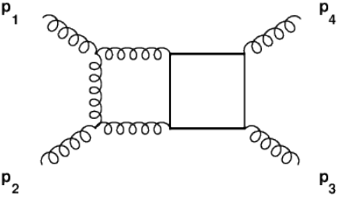
Refer to caption
Figure 10: Four points two-loop diagram

Let us consider the four point two-loop integral depicted on Fig. 10. This diagram has recently been computed in ref. Becchetti:2017abb in the context of top-mass corrections to 2​j2j or 2​γ2\gamma production.
The external kinematics is as in the previous section. The set of propagators reads:

D1=k12,D2=(k1+p1)2,D3=(k1−p3−p4)2,D4=(k2−p3−p4)2−m2,\displaystyle D_{1}=k_{1}^{2},\;\;\;D_{2}=(k_{1}+p_{1})^{2},\;\;\;D_{3}=(k_{1}-p_{3}-p_{4})^{2},\;\;\;D_{4}=(k_{2}-p_{3}-p_{4})^{2}-m^{2},
D5=(k2−p4)2−m2,D6=k22−m2,D7=(k1−k2)2−m2,\displaystyle D_{5}=(k_{2}-p_{4})^{2}-m^{2},\;\;\;D_{6}=k_{2}^{2}-m^{2},\;\;\;D_{7}=(k_{1}-k_{2})^{2}-m^{2}\,, (336)

while the additional ISP is :

z=D8=(k1−p4)2.\displaystyle z=D_{8}=(k_{1}-p_{4})^{2}. (337)

With Loop-by-Loop Baikov parametrization we have two options, we can either integrate the massive or the mass-less loop out first. Starting with the massless loop gives four master integrals in agreement with ref. Becchetti:2017abb and most public IBP codes. However, starting with the massive one, the number of master integrals is 3 : In this case, we get,

u\displaystyle u =(z−t)d−5(z+s)(4−d)/2(4m2s+(4m2−s)z)(d−5)/2z−1/2,\displaystyle=(z-t)^{d-5}\,(z+s)^{(4-d)/2}\,(4m^{2}s+(4m^{2}-s)z)^{(d-5)/2}\,z^{-1/2}\ , (338)

corresponding to

ω\displaystyle\omega =q0+q1​z+q2​z2+q3​z32​z​(s+z)​(z−t)​(4​m2​s+(4​m2−s)​z)​d​z,\displaystyle=\frac{q_{0}+q_{1}z+q_{2}z^{2}+q_{3}z^{3}}{2z(s+z)(z-t)(4m^{2}s+(4m^{2}-s)z)}dz\ , (339)

with

q0\displaystyle q_{0} =4​m2​s2​t,\displaystyle=4m^{2}s^{2}t\ ,
q1\displaystyle q_{1} =s⁡((d−6)​s​t+4​m2​((2​d−11)​s+3​t)),\displaystyle=s((d-6)st+4m^{2}((2d-11)s+3t))\ ,
q2\displaystyle q_{2} =(4​(4​d−23)​m2​s+(16−3​d)​s2+8​m2​t−2​s​t),\displaystyle=(4(4d-23)m^{2}s+(16-3d)s^{2}+8m^{2}t-2st)\ , (340)
q3\displaystyle q_{3} =2​(d−6)​(4​m2−s),\displaystyle=2(d-6)(4m^{2}-s)\ ,

and here it is easy to see that ω=0\omega=0 has three solutions, corresponding to ν=3\nu=3 master integrals for this sector.

We can get 3 master integrals out of the public code Kira 1.1 Maierhoefer:2017hyi if we also search for relations in sectors in which the ISP zz is allowed to appear as a propagator. What is happening is the following: Picking as master integrals in the seven-propagator sector defined by eqs. (336), the four integrals

I1111111;0,I1211111;0,I1111211;0,I1111112;0,\displaystyle I_{1111111;0}\,,\;\;I_{1211111;0}\,,\;\;I_{1111211;0}\,,\;\;I_{1111112;0}\,, (341)

Kira finds the relation

I0111121;1\displaystyle I_{0111121;1} =12​I1111112;0−12​I1111211;0−d−44​m2​I1111011;1+d−44​m2​I1111110;1+subtopologies,\displaystyle=\tfrac{1}{2}I_{1111112;0}-\tfrac{1}{2}I_{1111211;0}-\tfrac{d-4}{4m^{2}}I_{1111011;1}+\tfrac{d-4}{4m^{2}}I_{1111110;1}+\text{subtopologies}, (342)

where “subtopologies” refers to integrals in sectors with less than seven propagators. This relation is an example of an IBP relation that relate different sectors with the same number of propagators (what is referred to as a “magic relation” in ref. Maierhofer:2018gpa). On the cut of the first seven propagators, this identity reduces to

I1111112;0\displaystyle I_{1111112;0} =I1111211;0,\displaystyle=I_{1111211;0}\,, (343)

which is the relation that reduces the number of master integrals in this sector to 3 on the hepta-cut. We have verified this number with a numerical evaluation of the integrals combined with the high-precision arithmetic PSLQ algorithm Bailey09pslq:an (80 digits accuracy).

Proceeding with the reduction-by-intersections starting from the ω\omega of eq. (339), the decomposition formulas are in agreement with Kira.

For more discussion of this sector, see appendix A.2.

13 Two-Loop Bhabha Scattering

In this section, we discuss the seven-propagator sectors that contribute to Bhabha scattering (i.e. e+​e−→e+​e−e^{+}e^{-}\rightarrow e^{+}e^{-} in QED) at two loops. We take the external electrons to be on-shell so the integrals are functions of three variables s=(p1+p2)2s=(p_{1}+p_{2})^{2}, t=(p2+p3)2t=(p_{2}+p_{3})^{2}, and m2=pi2m^{2}=p_{i}^{2}. There are three such seven-propagator sectors, two planar and one non-planar.

13.1 First Planar Sector

Refer to caption
Figure 11: Bhabha - First planar sector.

This planar sector is depicted on Fig. 11, and was first computed in ref. Henn:2013woa. It may be expressed in terms of the seven propagators

D1=k22−m2,D2=(k2+p1)2,D3=(k2+p1+p2)2−m2,D4=(k1+p1+p2)2−m2,\displaystyle D_{1}=k_{2}^{2}-m^{2},\quad D_{2}=(k_{2}{+}p_{1})^{2},\quad D_{3}=(k_{2}+p_{1}+p_{2})^{2}-m^{2},\quad D_{4}=(k_{1}{+}p_{1}{+}p_{2})^{2}{-}m^{2},
D5=(k1+p1+p2+p3)2,D6=k12−m2,D7=(k1−k2)2.\displaystyle D_{5}=(k_{1}+p_{1}+p_{2}+p_{3})^{2},\quad D_{6}=k_{1}^{2}-m^{2},\quad D_{7}=(k_{1}-k_{2})^{2}. (344)

Additionally we need the variable z=D8=(k1+p1)2z=D_{8}=(k_{1}+p_{1})^{2}, which play the roles of ISP and eighth integration variable.

Using the Loop-by-Loop form of Baikov representation, by first integrating out k2k_{2}, we obtain:

u\displaystyle u =(z+s−4​m2)(4−d)/2​(z−t)d−5​z(d−6)/2,\displaystyle=(z+s-4m^{2})^{(4-d)/2}(z-t)^{d-5}z^{(d-6)/2}\,, (345)
ω\displaystyle\omega =(d−6)​(4​m2−s)​t+(2​t−(3​d−16)​(4​m2−s))​z+2​(d−6)​z22​z​(z+s−4​m2)​(z−t)​d​z,\displaystyle=\frac{(d-6)(4m^{2}-s)t+(2t-(3d-16)(4m^{2}-s))z+2(d-6)z^{2}}{2z(z+s-4m^{2})(z-t)}\,dz\,, (346)
ν\displaystyle\nu =2,𝒫={0,4​m2−s,t,∞}.\displaystyle=2\,,\quad\quad\quad\quad\quad\quad\mathcal{P}=\{0\,,4m^{2}-s\,,t\,,\infty\}\,. (347)
Mixed Bases.

Let us consider the decomposition of I1,1,1,1,1,1,1;−1=⟨ϕ2|𝒞]I_{1,1,1,1,1,1,1;-1}=\langle{\phi_{2}}|\mathcal{C}].
The MIs can be chosen as:

J1=I1,1,1,1,1,1,1;0=⟨e1|𝒞],J2=I1,1,1,1,1,1,2;0=⟨e2|𝒞],J_{1}=I_{1,1,1,1,1,1,1;0}=\langle{e_{1}}|\mathcal{C}]\,,\quad J_{2}=I_{1,1,1,1,1,1,2;0}=\langle{e_{2}}|\mathcal{C}],\, (348)

with:

e^1=1,e^2=5−dz.\displaystyle\hat{e}_{1}=1\,,\quad\hat{e}_{2}=\frac{5-d}{z}\,. (349)

We introduce the dlog differential-stripped cocycles:

φ^1=1z−1z−t,φ^2=1z−t−1z+s−4​m2.\displaystyle\hat{\varphi}_{1}=\frac{1}{z}-\frac{1}{z-t}\,,\quad\hat{\varphi}_{2}=\frac{1}{z-t}-\frac{1}{z+s-4m^{2}}\,. (350)

We can compute the 𝐂\mathbf{C} matrix:

𝐂i​j=⟨ei|φj⟩,i,j=1,2,\mathbf{C}_{ij}=\bra{e_{i}}\ket{\varphi_{j}}\,,\quad i,j=1,2\,, (351)

with:

⟨e1|φ1⟩\displaystyle\bra{e_{1}}\ket{\varphi_{1}} =td−5,⟨e1|φ2⟩=4​m2−s−td−5,\displaystyle=\frac{t}{d-5}\,,\quad\hskip 28.45274pt\bra{e_{1}}\ket{\varphi_{2}}=\frac{4m^{2}-s-t}{d-5}\,, (352)
⟨e2|φ1⟩\displaystyle\bra{e_{2}}\ket{\varphi_{1}} =−2​(d−5)d−6,⟨e2|φ2⟩=0.\displaystyle=\frac{-2(d-5)}{d-6}\,,\quad\;\,\bra{e_{2}}\ket{\varphi_{2}}=0\,. (353)

Moreover we can compute the intersection numbers:

⟨ϕ2|φ1⟩=(4​m2−s)​t2​(d−5),⟨ϕ2|φ2⟩=(3​d−14)​(4​m2−s)​(4​m2−s−t)2​(d−5)​(d−4).\displaystyle\bra{\phi_{2}}\ket{\varphi_{1}}=\frac{(4m^{2}-s)t}{2(d-5)}\,,\quad\bra{\phi_{2}}\ket{\varphi_{2}}=\frac{(3d-14)(4m^{2}-s)(4m^{2}-s-t)}{2(d-5)(d-4)}\,. (354)

The final reduction, given by eq. (48) is:

I1,1,1,1,1,1,1;−1=c1​J1+c2​J2I_{1,1,1,1,1,1,1;-1}=c_{1}\,J_{1}+c_{2}\,J_{2} (355)

with:

c1=(3​d−14)​(4​m2−s)2​(d−4),c2=(d−6)​(4​m2−s)​t2​(d−5)​(d−4),c_{1}=\frac{(3d-14)(4m^{2}-s)}{2(d-4)}\,,\quad c_{2}=\frac{(d-6)(4m^{2}-s)t}{2(d-5)(d-4)}\,, (356)

in agreement with FIRE.

13.2 Second Planar Sector

Refer to caption
Figure 12: Bhabha - second planar sector.

The second planar seven-propagator sector contributing to Bhabha scattering, shown in Fig. 12, can be expressed in terms of the propagators

D1=k22,D2=(k2+p1)2−m2,D3=(k2+p1+p2)2,D4=(k1+p1+p2)2−m2,\displaystyle D_{1}=k_{2}^{2},\;\;D_{2}=(k_{2}+p_{1})^{2}-m^{2},\;\;D_{3}=(k_{2}+p_{1}+p_{2})^{2},\;\;D_{4}=(k_{1}+p_{1}+p_{2})^{2}-m^{2},
D5=(k1+p1+p2+p3)2,D6=k12−m2,D7=(k1−k2)2−m2.\displaystyle D_{5}=(k_{1}+p_{1}+p_{2}+p_{3})^{2},\;\;D_{6}=k_{1}^{2}-m^{2},\;\;D_{7}=(k_{1}-k_{2})^{2}-m^{2}. (357)

We also need the ISP variable z=D8=(k1+p1)2z=D_{8}=(k_{1}+p_{1})^{2}.

After using the Loop-by-Loop Baikov representation and the hepta-cut, we get

u=\displaystyle u= (4m2−z)(d−5)/2(4m2−s−z)(4−d)/2(t−z)d−5z−1/2,\displaystyle\;(4m^{2}-z)^{(d-5)/2}(4m^{2}-s-z)^{(4-d)/2}(t-z)^{d-5}z^{-1/2}\,, (358)
ω=\displaystyle\omega= (4​m2​(4​m2−s)​t+(4​(2​d−11)​m2​(4​m2−s)−(12​m2+(d−6)​s)​t)​z2​z​(4​m2−z)​(4​m2−s−z)​(z−t)CLOSE\displaystyle\Big(\frac{4m^{2}(4m^{2}-s)t+(4(2d-11)m^{2}(4m^{2}-s)-(12m^{2}+(d-6)s)t)z}{2z(4m^{2}-z)(4m^{2}-s-z)(z-t)}
OPEN+((92−16​d)​m2+(3​d−16)​s+2​t)​z2+2​(d−6)​z32​z​(4​m2−z)​(4​m2−s−z)​(z−t))​d​z,\displaystyle+\frac{((92-16d)m^{2}+(3d-16)s+2t)z^{2}+2(d-6)z^{3}}{2z(4m^{2}-z)(4m^{2}-s-z)(z-t)}\Big)dz\,, (359)
ν\displaystyle\nu =3,𝒫={0,4​m2,4​m2−s,t,∞}.\displaystyle=3\,,\quad\quad\quad\quad\quad\quad\mathcal{P}=\{0\,,4m^{2}\,,4m^{2}-s\,,t\,,\infty\}\,. (360)
Mixed Bases.

Let us consider the decomposition of I1,1,1,1,1,1,1;−1I_{1,1,1,1,1,1,1;-1} in terms of the three master integrals

J1=I1,1,1,1,1,1,1;0=⟨e1|𝒞],J2=I1,1,1,1,2,1,1;0=⟨e2|𝒞],J3=I1,1,1,1,1,2,1;0=⟨e3|𝒞],\displaystyle J_{1}=I_{1,1,1,1,1,1,1;0}=\langle{e_{1}}|\mathcal{C}]\,,\quad J_{2}=I_{1,1,1,1,2,1,1;0}=\langle{e_{2}}|\mathcal{C}]\,,\quad J_{3}=I_{1,1,1,1,1,2,1;0}=\langle{e_{3}}|\mathcal{C}]\,, (361)

with:

e^1=1,e^2=(5−d)​((4​m2−s)​t+(4​m2−s−2​t)​z)(4​m2−s)​(t−z)2,\displaystyle\hat{e}_{1}=1\,,\qquad\hat{e}_{2}=\frac{(5-d)((4m^{2}-s)t+(4m^{2}-s-2t)z)}{(4m^{2}-s)(t-z)^{2}}\,, (362)
e^3=(d−6)​(4​m2−s)​t+((d−4)​(4​m2−s)−2​(d−5)​t)​z2​(4​m2−s)​(4​m2−s−z)​(t−z).\displaystyle\quad\hat{e}_{3}=\frac{(d-6)(4m^{2}-s)t+((d-4)(4m^{2}-s)-2(d-5)t)z}{2(4m^{2}-s)(4m^{2}-s-z)(t-z)}\,. (363)

The dlog differential-stripped cocycles reads:

φ^1=1z−1z−4​m2,φ^2=1z−4​m2−1z+s−4​m2,φ^3=1z+s−4​m2−1z−t.\displaystyle\hat{\varphi}_{1}=\frac{1}{z}-\frac{1}{z{-}4m^{2}},\;\;\;\hat{\varphi}_{2}=\frac{1}{z{-}4m^{2}}-\frac{1}{z{+}s{-}4m^{2}},\;\;\;\hat{\varphi}_{3}=\frac{1}{z{+}s{-}4m^{2}}-\frac{1}{z{-}t}\,. (364)

We can compute the 𝐂\mathbf{C} matrix:

𝐂i​j=⟨ei|φj⟩,i,j=1,2,\mathbf{C}_{ij}=\bra{e_{i}}\ket{\varphi_{j}}\,,\quad i,j=1,2\,, (365)

with:

⟨e1|φ1⟩=4​m2d−5,⟨e1|φ2⟩=−sd−5,⟨e1|φ3⟩=s+t−4​m2d−5,⟨e2|φ1⟩=8​(d−5)​m2​(s+t−4​m2)(d−6)​(4​m2−s)​(4​m2−t),⟨e2|φ2⟩=2​(5−d)​s​t(d−6)​(4​m2−s)​(4​m2−t),⟨e2|φ3⟩=4​(d−5)​m2​(4​m2−s−t)(d−6)​(4​m2−s)​(4​m2−t),⟨e3|φ1⟩=0,⟨e3|φ2⟩=1,⟨e3|φ3⟩=−4​m2−s−t4​m2−s.\begin{split}\bra{e_{1}}\ket{\varphi_{1}}&=\frac{4m^{2}}{d-5}\,,\quad\hskip 28.45274pt\bra{e_{1}}\ket{\varphi_{2}}=\frac{-s}{d-5}\,,\quad\hskip 28.45274pt\bra{e_{1}}\ket{\varphi_{3}}=\frac{s+t-4m^{2}}{d-5}\,,\\ \bra{e_{2}}\ket{\varphi_{1}}&=\frac{8(d-5)m^{2}(s+t-4m^{2})}{(d-6)(4m^{2}-s)(4m^{2}-t)}\,,\quad\bra{e_{2}}\ket{\varphi_{2}}=\frac{2(5-d)st}{(d-6)(4m^{2}-s)(4m^{2}-t)}\,,\\ &\qquad\qquad\qquad\bra{e_{2}}\ket{\varphi_{3}}=\frac{4(d-5)m^{2}(4m^{2}-s-t)}{(d-6)(4m^{2}-s)(4m^{2}-t)}\,,\\ \bra{e_{3}}\ket{\varphi_{1}}&=0\,,\quad\hskip 28.45274pt\bra{e_{3}}\ket{\varphi_{2}}=1\,,\quad\hskip 28.45274pt\bra{e_{3}}\ket{\varphi_{3}}=-\frac{4m^{2}-s-t}{4m^{2}-s}\,.\end{split} (366)

The additional intersection numbers are

⟨ϕ2|φ1⟩\displaystyle\langle\phi_{2}|\varphi_{1}\rangle =2​m2​(4​(2​d−9)−m2​(d−4)​s−2​(d−5)​t)(d−5)​(d−4),\displaystyle=\frac{2m^{2}\,(4(2d-9)-m^{2}(d-4)s-2(d-5)t)}{(d-5)(d-4)}\,,
⟨ϕ2|φ2⟩\displaystyle\langle\phi_{2}|\varphi_{2}\rangle =s⁡((76−16​d)​m2+(3​d−14)​s+2​(d−5)​t)2​(d−5)​(d−4),\displaystyle=\frac{s\,((76-16d)m^{2}+(3d-14)s+2(d-5)t)}{2(d-5)(d-4)}\,, (367)
⟨ϕ2|φ3⟩\displaystyle\langle\phi_{2}|\varphi_{3}\rangle =(4​(9−2​d)​m2+(3​d−14)​s)​(4​m2−s−t)2​(d−5)​(d−4),\displaystyle=\frac{(4(9-2d)m^{2}+(3d-14)s)\,(4m^{2}-s-t)}{2(d-5)(d-4)}\,,

The final reduction, given by eq. (48) is:

I1,1,1,1,1,1,1;−1=c1​J1+c2​J2+c3​J3I_{1,1,1,1,1,1,1;-1}=c_{1}\,J_{1}+c_{2}\,J_{2}+c_{3}\,J_{3} (368)

with:

c1=−8​(9−2​d)​m4+(d−6)​s​t+2​(d−4)​m2​(s+2​t)2​(d−4)​(2​m2−t),\displaystyle c_{1}=-\frac{8(9-2d)m^{4}+(d-6)st+2(d-4)m^{2}(s+2t)}{2(d-4)(2m^{2}-t)}\,, (369)
c2=(d−6)​(4​m2−s)​(4​m2−t)​t2​(d−5)​(d−4)​(2​m2−t)c3=−2​(4​m2−s)​s​(m2−t)(d−4)​(2​m2−t),\displaystyle\quad c_{2}=\frac{(d-6)\,(4m^{2}-s)\,(4m^{2}-t)\,t}{2(d-5)(d-4)(2m^{2}-t)}\,\quad c_{3}=-\frac{2\,(4m^{2}-s)\,s\,(m^{2}-t)}{(d-4)(2m^{2}-t)}, (370)

in agreement with Kira.

13.3 Non-Planar Sector

Refer to caption
Figure 13: Bhabha non-planar sector.

We consider the non-planar contribution to Bhabha scattering in Fig. 13. The seven denominators can be parametrized as:

D1=k22−m2,D2=(k2+p1)2,D3=(k1+p1+p2)2−m2,D4=(k1+p1+p2+p3)2,\displaystyle D_{1}=k_{2}^{2}-m^{2},\;\;D_{2}=(k_{2}+p_{1})^{2},\;\;D_{3}=(k_{1}+p_{1}+p_{2})^{2}-m^{2},\;\;D_{4}=(k_{1}+p_{1}+p_{2}+p_{3})^{2},
D5=k12−m2,D6=(k1−k2)2,D7=(k1−k2+p2)2−m2,\displaystyle D_{5}=k_{1}^{2}-m^{2},\;\;D_{6}=(k_{1}-k_{2})^{2},\;\;D_{7}=(k_{1}-k_{2}+p_{2})^{2}-m^{2}\,, (371)

and the leftover ISP is:

z=D8=(k1+p1)2.z=D_{8}=(k_{1}+p_{1})^{2}. (372)

We find:

u\displaystyle u =(z−t)d−5z(d−6)/2(z+s)(d−5)/2(z+s−4m2)−1/2\displaystyle=(z-t)^{d-5}\,z^{(d-6)/2}\,(z+s)^{(d-5)/2}\,(z+s-4m^{2})^{-1/2}\, (373)
ω\displaystyle\omega =c0+c1​z+c2​z2+c3​z32​z​(z+s)​(s+z−4​m2)​(z−t)​d​z\displaystyle=\frac{c_{0}+c_{1}z+c_{2}z^{2}+c_{3}z^{3}}{2z(z+s)(s+z-4m^{2})(z-t)}\,dz (374)

where in eq. (374) we defined:

c0\displaystyle c_{0} =(d−6)​(4​m2−s)​s​t,\displaystyle=(d-6)(4m^{2}-s)st\,,
c1\displaystyle c_{1} =(3​d−16)​s​(s−4​m2)+(8​d−44)​m2​t−3​(d−6)​s​t,\displaystyle=(3d-16)s(s-4m^{2})+(8d-44)m^{2}t-3(d-6)st\,,
c2\displaystyle c_{2} =(84−16​d)​m2+(7​d−38)​s−2​(d−6)​t,\displaystyle=(84-16d)m^{2}+(7d-38)s-2(d-6)t\,, (375)
c3\displaystyle c_{3} =(4​d−22),\displaystyle=(4d-22)\,,

and so, we get:

ν\displaystyle\nu =3,𝒫={0,−s,4​m2−s,t}.\displaystyle=3\,,\quad\mathcal{P}=\{0\,,-s\,,4m^{2}-s\,,t\}\,. (376)
Mixed Bases

Let us consider the decomposition of I1,1,1,1,1,1,1;−1=⟨ϕ2|𝒞]I_{1,1,1,1,1,1,1;-1}=\langle{\phi_{2}}|\mathcal{C}].
The MIs can be chosen as:

J1=I1,1,1,1,1,1,1;0=⟨e1|𝒞],J2=I1,1,1,1,1,2,1;0=⟨e2|𝒞],J3=I1,1,1,1,1,1,2;0=⟨e3|𝒞],J_{1}=I_{1,1,1,1,1,1,1;0}=\langle{e_{1}}|\mathcal{C}]\,,\quad J_{2}=I_{1,1,1,1,1,2,1;0}=\langle{e_{2}}|\mathcal{C}]\,,\quad J_{3}=I_{1,1,1,1,1,1,2;0}=\langle{e_{3}}|\mathcal{C}]\,, (377)

with:

e^1=1,e^2\displaystyle\hat{e}_{1}=1\,,\quad\hat{e}_{2} =5−dz,e^3=d−5z+s.\displaystyle=\frac{5-d}{z}\,,\quad\hat{e}_{3}=\frac{d-5}{z+s}\,. (378)

Moreover we introduce the following dlog differential-stripped cocycles:

φ^1\displaystyle\hat{\varphi}_{1} =1z−1z+s−4​m2,\displaystyle=\frac{1}{z}-\frac{1}{z+s-4m^{2}}\,, (379)
φ^2\displaystyle\hat{\varphi}_{2} =1z+s−4​m2−1z+s,\displaystyle=\frac{1}{z+s-4m^{2}}-\frac{1}{z+s}\,, (380)
φ^3\displaystyle\hat{\varphi}_{3} =1z+s−1z−t\displaystyle=\frac{1}{z+s}-\frac{1}{z-t} (381)

We compute the 𝐂\mathbf{C} matrix:

𝐂i​j=⟨ei|φj⟩,1≤i,j≤3,\mathbf{C}_{ij}=\bra{e_{i}}\ket{\varphi_{j}}\,,\quad 1\leq i,j\leq 3, (382)

with:

⟨e1|φ1⟩\displaystyle\langle e_{1}|\varphi_{1}\rangle =4​m2−s2​(d−5),\displaystyle=\frac{4m^{2}-s}{2(d-5)}\,, ⟨e1|φ2⟩\displaystyle\langle e_{1}|\varphi_{2}\rangle =2​m25−d,\displaystyle=\frac{2m^{2}}{5-d}\,, ⟨e1|φ3⟩\displaystyle\langle e_{1}|\varphi_{3}\rangle =s+t2​(d−5),\displaystyle=\frac{s+t}{2(d-5)}\,, (383)
⟨e2|φ1⟩\displaystyle\langle e_{2}|\varphi_{1}\rangle =2​(5−d)d−6,\displaystyle=\frac{2(5-d)}{d-6}\,, ⟨e2|φ2⟩\displaystyle\langle e_{2}|\varphi_{2}\rangle =0,\displaystyle=0\,, ⟨e2|φ3⟩\displaystyle\langle e_{2}|\varphi_{3}\rangle =0,\displaystyle=0\,, (384)
⟨e3|φ1⟩\displaystyle\langle e_{3}|\varphi_{1}\rangle =0,\displaystyle=0\,, ⟨e3|φ2⟩\displaystyle\langle e_{3}|\varphi_{2}\rangle =−2,\displaystyle=-2\,, ⟨e3|φ3⟩\displaystyle\langle e_{3}|\varphi_{3}\rangle =2.\displaystyle=2\,. (385)

Moreover we can compute the intersection numbers:

⟨ϕ2|φ1⟩\displaystyle\langle\phi_{2}|\varphi_{1}\rangle =(4​m2−s)​(4​(4​d−19)​m2+(14−3​d)​s−2​(d−5)​t)4​(d−5)​(2​d−9),\displaystyle=\frac{(4m^{2}-s)(4(4d-19)m^{2}+(14-3d)s-2(d-5)t)}{4(d-5)(2d-9)}\,, (386)
⟨ϕ2|φ2⟩\displaystyle\langle\phi_{2}|\varphi_{2}\rangle =m2​((76−16​d)​m2+(7​d−34)​s+2​(d−5)​t)(d−5)​(2​d−9),\displaystyle=\frac{m^{2}((76-16d)m^{2}+(7d-34)s+2(d-5)t)}{(d-5)(2d-9)}\,, (387)
⟨ϕ2|φ3⟩\displaystyle\langle\phi_{2}|\varphi_{3}\rangle =(s+t)​(4​m2+(14−3​d)​s+2​(d−5)​t)4​(d−5)​(2​d−9).\displaystyle=\frac{(s+t)(4m^{2}+(14-3d)s+2(d-5)t)}{4(d-5)(2d-9)}\,. (388)

Then, eq. (48) yields:

I1,1,1,1,1,1,1;−1=c1​J1+c2​J2+c3​J3,I_{1,1,1,1,1,1,1;-1}=c_{1}J_{1}+c_{2}J_{2}+c_{3}J_{3}\,, (389)

with:

c1\displaystyle c_{1} =4​(4​d−19)​m2+(14−3​d)​s+2​(d−5)​t4​d−18,\displaystyle=\frac{4(4d{-}19)m^{2}{+}(14{-}3d)s{+}2(d{-}5)t}{4d{-}18}\,, (390)
c2\displaystyle c_{2} =(d−6)​(4​m2−s)​t2​(d−5)​(2​d−9),\displaystyle=\frac{(d{-}6)(4m^{2}{-}s)t}{2(d{-}5)(2d{-}9)}\,, (391)
c3\displaystyle c_{3} =−2​m2​(s+t)2​d−9,\displaystyle=\frac{{-}2m^{2}(s{+}t)}{2d{-}9}\,, (392)

in agreement with Kira.

14 Two-Loop Associated Higgs Production

14.1 Planar Contribution to H+jH{+}j and H​HHH Production

Refer to caption
Refer to caption
Figure 14: A planar contribution to H+jH{+}j (left) and to H​HHH (right).

In this section we discuss planar seven-propagator integrals contributing to Higgs+jet (H+jH{+}j) production Melnikov:2016qoc; Bonciani:2016qxi; Jones:2018hbb and double Higgs (H​HHH) production Borowka:2016ypz; Baglio:2018lrj, portrayed in Fig. 14. We treat the two cases simultaneously as they are very similar. The seven propagators are

D1=k22−mt2,D2=(k2+p1)2−mt2,D3=(k2+p1+p2)2−mt2,D4=(k1+p1+p2)2−mt2,\displaystyle D_{1}=k_{2}^{2}-m_{t}^{2},\;\;D_{2}=(k_{2}{+}p_{1})^{2}-m_{t}^{2},\;\;D_{3}=(k_{2}{+}p_{1}{+}p_{2})^{2}-m_{t}^{2},\;\;D_{4}=(k_{1}{+}p_{1}{+}p_{2})^{2}{-}m_{t}^{2},
D5=(k1+p1+p2+p3)2−mt2,D6=k12−mt2,D7=(k1−k2)2.\displaystyle D_{5}=(k_{1}{+}p_{1}{+}p_{2}{+}p_{3})^{2}-m_{t}^{2},\qquad D_{6}=k_{1}^{2}-m_{t}^{2},\qquad D_{7}=(k_{1}{-}k_{2})^{2}. (393)

The ISP is chosen to be:

z=D8=(k1+p1)2−mt2z=D_{8}=(k_{1}{+}p_{1})^{2}-m_{t}^{2} (394)

The kinematics is such that p12=p22=0p_{1}^{2}=p_{2}^{2}=0, (p1+p2)2=s(p_{1}+p_{2})^{2}=s, (p2+p3)2=t(p_{2}+p_{3})^{2}=t, and (p1+p2+p3)2=mH2(p_{1}+p_{2}+p_{3})^{2}=m_{H}^{2}. The only difference between the cases of H+jH{+}j and H​HHH is the relation p32=δ​mH2p_{3}^{2}=\delta m_{H}^{2} where δ=0\delta=0 for the case of H+jH{+}j, while δ=1\delta=1 for the case of H​HHH.
The Loop-by-Loop Baikov parametrization, on the maximal cut, gives us:

u\displaystyle u =zd−5​((z−r1)​(z−r2))(4−d)/2​((z−r3)​(z−r4))(d−5)/2,\displaystyle=z^{d-5}((z-r_{1})(z-r_{2}))^{(4-d)/2}((z-r_{3})(z-r_{4}))^{(d-5)/2}\,, (395)

with:

r1=\displaystyle r_{1}= 12​(−s2−4​s​mt2−s),\displaystyle\frac{1}{2}\left(-\sqrt{s^{2}-4sm_{t}^{2}}-s\right)\,, (396)
r2=\displaystyle r_{2}= 12​(s2−4​s​mt2−s),\displaystyle\frac{1}{2}\left(\sqrt{s^{2}-4sm_{t}^{2}}-s\right)\,, (397)
r3=\displaystyle r_{3}= (2​s⁡(δ​mH4−(δ+1)​t​mH2+t⁡(s+t))​(mH4​((δ−1)2​mt2+δ​s)−2​(δ+1)​s​mH2​mt2+s2​mt2)+CLOSE\displaystyle\Big(2\sqrt{s\left(\delta m_{H}^{4}-(\delta+1)tm_{H}^{2}+t(s+t)\right)\left(m_{H}^{4}\left((\delta-1)^{2}m_{t}^{2}+\delta s\right)-2(\delta+1)sm_{H}^{2}m_{t}^{2}+s^{2}m_{t}^{2}\right)}+
OPEN2​δ​s​mH4−(δ+1)​s​t​mH2+s2​t)/((δ−1)2​mH4−2​(δ+1)​s​mH2+s2),\displaystyle 2\delta sm_{H}^{4}-(\delta+1)stm_{H}^{2}+s^{2}t\Big)/\Big((\delta-1)^{2}m_{H}^{4}-2(\delta+1)sm_{H}^{2}+s^{2}\Big)\,, (398)
r4=\displaystyle r_{4}= (−2​s⁡(δ​mH4−(δ+1)​t​mH2+t⁡(s+t))​(mH4​((δ−1)2​mt2+δ​s)−2​(δ+1)​s​mH2​mt2+s2​mt2)+CLOSE\displaystyle\Big(-2\sqrt{s\left(\delta m_{H}^{4}-(\delta+1)tm_{H}^{2}+t(s+t)\right)\left(m_{H}^{4}\left((\delta-1)^{2}m_{t}^{2}+\delta s\right)-2(\delta+1)sm_{H}^{2}m_{t}^{2}+s^{2}m_{t}^{2}\right)}+
OPEN2​δ​s​mH4−(δ+1)​s​t​mH2+s2​t)/((δ−1)2​mH4−2​(δ+1)​s​mH2+s2).\displaystyle 2\delta sm_{H}^{4}-(\delta+1)stm_{H}^{2}+s^{2}t\Big)/\Big((\delta-1)^{2}m_{H}^{4}-2(\delta+1)sm_{H}^{2}+s^{2}\Big)\,. (399)

Then, we have:

ω\displaystyle\omega =q0+q1​z+q2​z2+q3​z3+q4​z42​z​(z−r1)​(z−r2)​(z−r3)​(z−r4)​d​z\displaystyle=\frac{q_{0}+q_{1}z+q_{2}z^{2}+q_{3}z^{3}+q_{4}z^{4}}{2z(z-r_{1})(z-r_{2})(z-r_{3})(z-r_{4})}dz (400)

where:

q0=2​(d−5)​r1​r2​r3​r4,\displaystyle q_{0}=2(d-5)r_{1}r_{2}r_{3}r_{4}\,, (401)
q1=−((d−6)​(r1+r2)​r3​r4+3​(d−5)​r1​r2​(r3+r4)),\displaystyle q_{1}=-((d-6)(r_{1}+r_{2})r_{3}r_{4}+3(d-5)r_{1}r_{2}(r_{3}+r_{4}))\,, (402)
q2=4​(d−5)​r1​r2−2​r3​r4+(2​d−11)​(r1+r2)​(r3+r4),\displaystyle q_{2}=4(d-5)r_{1}r_{2}-2r_{3}r_{4}+(2d-11)(r_{1}+r_{2})(r_{3}+r_{4})\,, (403)
q3=((16−3​d)​(r1+r2)−(d−7)​(r3+r4)),\displaystyle q_{3}=((16-3d)(r_{1}+r_{2})-(d-7)(r_{3}+r_{4}))\,, (404)
q4=2​(d−6).\displaystyle q_{4}=2(d-6)\,. (405)

Therefore we find:

ν=4,𝒫={0,r1,r2,r3,r4​∞}.\nu=4\,,\quad\mathcal{P}=\{0,r_{1}\,,r_{2}\,,r_{3}\,,r_{4}\,\infty\}\,. (406)
Mixed Bases.

Let us consider the reduction of I1,1,1,1,1,1,1;−1=⟨ϕ2|𝒞]I_{1,1,1,1,1,1,1;-1}=\langle{\phi_{2}}|\mathcal{C}] in terms of J1=I1,1,1,1,1,1,1;0=⟨e1|𝒞]J_{1}=I_{1,1,1,1,1,1,1;0}=\langle{e_{1}}|\mathcal{C}], J2=I1,2,1,1,1,1,1;0=⟨e2|𝒞]J_{2}=I_{1,2,1,1,1,1,1;0}=\langle{e_{2}}|\mathcal{C}], J3=I1,1,1,1,2,1,1;0=⟨e3|𝒞]J_{3}=I_{1,1,1,1,2,1,1;0}=\langle{e_{3}}|\mathcal{C}] and J4=I1,1,1,1,1,1,2;0=⟨e4|𝒞]J_{4}=I_{1,1,1,1,1,1,2;0}=\langle{e_{4}}|\mathcal{C}] with:

e^1\displaystyle\hat{e}_{1} =1,\displaystyle=1\,, (407)
e^2\displaystyle\hat{e}_{2} =5−dz,\displaystyle=\frac{5-d}{z}\,, (408)
e^3\displaystyle\hat{e}_{3} =(d−5)​s​(((1+δ)​mH2−s−2​t)​z−s​t)((1−δ)2​mH4−2​(1+δ)​mH2​s+s2)​(z−r3)​(z−r4),\displaystyle=\frac{(d-5)\,s\,(((1+\delta)m_{H}^{2}-s-2t)z-st)}{((1-\delta)^{2}m_{H}^{4}-2(1+\delta)m_{H}^{2}s+s^{2})(z-r_{3})(z-r_{4})}\,, (409)
e^4\displaystyle\hat{e}_{4} =(d−5)​s​(2​mt2+z)(4​mt2−s)​z2.\displaystyle=\frac{(d-5)s(2m_{t}^{2}+z)}{(4m_{t}^{2}-s)z^{2}}\,. (410)

Moreover we can introduce the following differential-stripped cocycles:

φ^1\displaystyle\hat{\varphi}_{1} =1z−1z−r1,\displaystyle=\frac{1}{z}-\frac{1}{z{-}r_{1}}\,, φ^2\displaystyle\hat{\varphi}_{2} =1z−r1−1z−r2,\displaystyle=\frac{1}{z{-}r_{1}}-\frac{1}{z{-}r_{2}}\,,\qquad (411)
φ^3\displaystyle\hat{\varphi}_{3} =1z−r2−1z−r3,\displaystyle=\frac{1}{z{-}r_{2}}-\frac{1}{z{-}r_{3}}\,,\!\!\!\!\! φ^4\displaystyle\hat{\varphi}_{4} =1z−r3−1z−r4.\displaystyle=\frac{1}{z{-}r_{3}}-\frac{1}{z{-}r_{4}}\,. (412)

We compute the 𝐂\mathbf{C} matrix:

𝐂i​j=⟨ei|φj⟩,1≤i,j≤4,\mathbf{C}_{ij}=\bra{e_{i}}\ket{\varphi_{j}}\,,\quad 1\leq i,j\leq 4\,, (413)

with:

⟨e1|φ1⟩\displaystyle\bra{e_{1}}\ket{\varphi_{1}} =r1d−5,\displaystyle=\frac{r_{1}}{d-5}\,, ⟨e1|φ2⟩\displaystyle\bra{e_{1}}\ket{\varphi_{2}} =r2−r1d−5,\displaystyle=\frac{r_{2}-r_{1}}{d-5}\,, ⟨e1|φ3⟩\displaystyle\bra{e_{1}}\ket{\varphi_{3}} =r3−r2d−5,\displaystyle=\frac{r_{3}-r_{2}}{d-5}\,, (414)
⟨e1|φ4⟩\displaystyle\bra{e_{1}}\ket{\varphi_{4}} =r4−r3d−5,\displaystyle=\frac{r_{4}-r_{3}}{d-5}\,, ⟨e2|φ1⟩\displaystyle\bra{e_{2}}\ket{\varphi_{1}} =−1,\displaystyle=-1\,, ⟨e2|φ2⟩\displaystyle\bra{e_{2}}\ket{\varphi_{2}} =0,\displaystyle=0\,, (415)
⟨e2|φ3⟩=⟨e2|φ4⟩=⟨e3|φ1⟩=⟨e3|φ2⟩= 0,\displaystyle\bra{e_{2}}\ket{\varphi_{3}}\,=\,\bra{e_{2}}\ket{\varphi_{4}}\,=\,\bra{e_{3}}\ket{\varphi_{1}}\,=\,\bra{e_{3}}\ket{\varphi_{2}}\,=\,0\,, (416)
⟨e3|φ3⟩\displaystyle\bra{e_{3}}\ket{\varphi_{3}} =2​s​(s​t+r3​(s+2​t−(1+δ)​mH2))(r3−r4)​((1−δ)2​mH4−2​(1+δ)​mH2​s+s2),\displaystyle=\frac{2s(st+r_{3}(s+2t-(1+\delta)m_{H}^{2}))}{(r_{3}-r_{4})((1-\delta)^{2}m_{H}^{4}-2(1+\delta)m_{H}^{2}s+s^{2})}\,, (417)
⟨e3|φ4⟩\displaystyle\bra{e_{3}}\ket{\varphi_{4}} =2​s​((r3+r4)​((1+δ)​mH2−s−2​t)−2​s​t)(r3−r4)​((1−δ)2​mH4−2​(1+δ)​mH2​s+s2),\displaystyle=\frac{2s((r_{3}+r_{4})((1+\delta)m_{H}^{2}-s-2t)-2st)}{(r_{3}-r_{4})((1-\delta)^{2}m_{H}^{4}-2(1+\delta)m_{H}^{2}s+s^{2})}\,, (418)
⟨e4|φ1⟩\displaystyle\bra{e_{4}}\ket{\varphi_{1}} =s⁡[(d−6)​r1​r2​r3​r4+mt2​((d−6)​r2​r3​r4−(d−4)​r1​r3​r4+(d−5)​r1​r2​(r3+r4))](d−6)​r1​r2​r3​r4​(4​mt2−s),\displaystyle=\frac{s\,[(d-6)r_{1}r_{2}r_{3}r_{4}+m_{t}^{2}((d-6)r_{2}r_{3}r_{4}-(d-4)r_{1}r_{3}r_{4}+(d-5)r_{1}r_{2}(r_{3}+r_{4}))]}{(d-6)r_{1}r_{2}r_{3}r_{4}(4m_{t}^{2}-s)}\,, (419)
⟨e4|φ2⟩\displaystyle\bra{e_{4}}\ket{\varphi_{2}} =(r1−r2)r1​r2​2​(d−5)​mt2​s(d−6)​(4​mt2−s),\displaystyle=\frac{(r_{1}-r_{2})}{r_{1}r_{2}}\,\frac{2(d-5)m_{t}^{2}s}{(d-6)(4m_{t}^{2}-s)}\,, (420)
⟨e4|φ3⟩\displaystyle\bra{e_{4}}\ket{\varphi_{3}} =(r2−r3)r2​r3​2​(d−5)​mt2​s(d−6)​(4​mt2−s),\displaystyle=\frac{(r_{2}-r_{3})}{r_{2}r_{3}}\,\frac{2(d-5)m_{t}^{2}s}{(d-6)(4m_{t}^{2}-s)}\,, (421)
⟨e4|φ4⟩\displaystyle\bra{e_{4}}\ket{\varphi_{4}} =(r3−r4)r3​r4​2​(d−5)​mt2​s(d−6)​(4​mt2−s).\displaystyle=\frac{(r_{3}-r_{4})}{r_{3}r_{4}}\,\frac{2(d-5)m_{t}^{2}s}{(d-6)(4m_{t}^{2}-s)}\,. (422)

We notice that only two of the sixteen entries of 𝐂\mathbf{C} have explicit dependence on δ\delta.
Moreover we can compute the intersection numbers:

⟨ϕ2|φ1⟩\displaystyle\bra{\phi_{2}}\ket{\varphi_{1}} =r1​((3​d−14)​r1+(d−4)​r2−(d−5)​(r3+r4))2​(d−5)​(d−4),\displaystyle=\frac{r_{1}((3d-14)r_{1}+(d-4)r_{2}-(d-5)(r_{3}+r_{4}))}{2(d-5)(d-4)}\,, (423)
⟨ϕ2|φ2⟩\displaystyle\bra{\phi_{2}}\ket{\varphi_{2}} =(r2−r1)​((3​d−14)​(r1+r2)−(d−5)​(r3+r4))2​(d−5)​(d−4),\displaystyle=\frac{(r_{2}-r_{1})((3d-14)(r_{1}+r_{2})-(d-5)(r_{3}+r_{4}))}{2(d-5)(d-4)}\,, (424)
⟨ϕ2|φ3⟩\displaystyle\bra{\phi_{2}}\ket{\varphi_{3}} =(r3−r2)​((d−4)​r1+(3​d−14)​r2+(d−5)​(r3−r4))2​(d−5)​(d−4),\displaystyle=\frac{(r_{3}-r_{2})((d-4)r_{1}+(3d-14)r_{2}+(d-5)(r_{3}-r_{4}))}{2(d-5)(d-4)}\,, (425)
⟨ϕ2|φ4⟩\displaystyle\bra{\phi_{2}}\ket{\varphi_{4}} =(r4−r3)​((d−4)​(r1+r2)+(d−5)​(r3+r4))2​(d−5)​(d−4).\displaystyle=\frac{(r_{4}-r_{3})((d-4)(r_{1}+r_{2})+(d-5)(r_{3}+r_{4}))}{2(d-5)(d-4)}\,. (426)

From now on, we reintroduce the explicit values of δ\delta.

∙\bullet H+j reduction: (δ=0)(\delta=0).

The final reduction (48) reads:

I1,1,1,1,1,1,1;−1=c1​J1+c2​J2+c3​J3+c4​J4,I_{1,1,1,1,1,1,1;-1}=c_{1}J_{1}+c_{2}J_{2}+c_{3}J_{3}+c_{4}J_{4}\,, (427)

with:

c1\displaystyle c_{1} =s⁡((3​d−14)​(2​mT2​(mH2−s)−s​t)+4​(2​d−9)​mt2​t)2​(d−4)​(s​t+2​mt2​(mH2−s−2​t)),\displaystyle=\frac{s\,\big((3d-14)(2m_{T}^{2}(m_{H}^{2}-s)-st)+4(2d-9)m_{t}^{2}t\big)}{2(d-4)(st+2m_{t}^{2}(m_{H}^{2}-s-2t))}\,, (428)
c2\displaystyle c_{2} =2​mt2​s​(mt2​(mH2−s−2​t)+s​t)(d−4)​(s​t+2​mt2​(mH2−s−2​t)),\displaystyle=\frac{2m_{t}^{2}s(m_{t}^{2}(m_{H}^{2}-s-2t)+st)}{(d-4)(st+2m_{t}^{2}(m_{H}^{2}-s-2t))}\,, (429)
c3\displaystyle c_{3} =2​mt2​(s​t​(s+t−mH2)−mt2​(s+2​t−mH2)2)(d−4)​(s​t+2​mt2​(mH2−s−2​t)),\displaystyle=\frac{2m_{t}^{2}\big(st(s+t-m_{H}^{2})-m_{t}^{2}(s+2t-m_{H}^{2})^{2}\big)}{(d-4)(st+2m_{t}^{2}(m_{H}^{2}-s-2t))}, (430)
c4\displaystyle c_{4} =(d−6)​s​t​(s−4​mt2)​(4​mt2​(mH2−s−t)+s​t)2​(d−5)​(d−4)​(mH2−s)​(s​t+2​mt2​(mH2−s−2​t)).\displaystyle=\frac{(d-6)\,st\,(s-4m_{t}^{2})\,(4m_{t}^{2}(m_{H}^{2}-s-t)+st)}{2(d-5)(d-4)(m_{H}^{2}-s)(st+2m_{t}^{2}(m_{H}^{2}-s-2t))}\,. (431)

The result is in agreement with Kira.

∙\bullet HH production: (δ=1)(\delta=1).

The final reduction (48) reads:

I1,1,1,1,1,1,1;−1=c1​J1+c2​J2+c3​J3+c4​J4,I_{1,1,1,1,1,1,1;-1}=c_{1}J_{1}+c_{2}J_{2}+c_{3}J_{3}+c_{4}J_{4}\,, (432)

with:

c1\displaystyle c_{1} =s⁡((4​(d−5)​mH4−(3​d−14)​s​(4​mH2−s))​t−2​mt2​(4​mH2−s)​((3​d−14)​(2​mH2−s)+2​(9−2​d)​t))2​(d−4)​(4​mH2−s)​(2​mt2​(2​mH2−s−2​t)+s​t),\displaystyle=\frac{s\,\big((4(d{-}5)m_{H}^{4}{-}(3d{-}14)s(4m_{H}^{2}{-}s))t{-}2m_{t}^{2}(4m_{H}^{2}{-}s)((3d{-}14)(2m_{H}^{2}{-}s){+}2(9{-}2d)t)\big)}{2(d-4)(4m_{H}^{2}-s)(2m_{t}^{2}(2m_{H}^{2}-s-2t)+st)}\,, (433)
c2\displaystyle c_{2} =2​mt2​s​(mt2​(4​mH2−s)​(2​mH2−s−2​t)+2​mH4​(mH2−t)−s2​t−mH2​s​(mH2−4​t))(d−4)​(4​mH2−s)​(2​mt2​(2​mH2−s−2​t)+s​t),\displaystyle=\frac{2m_{t}^{2}s\,\big(m_{t}^{2}(4m_{H}^{2}-s)(2m_{H}^{2}-s-2t)+2m_{H}^{4}(m_{H}^{2}-t)-s^{2}t-m_{H}^{2}s(m_{H}^{2}-4t)\big)}{(d-4)(4m_{H}^{2}-s)(2m_{t}^{2}(2m_{H}^{2}-s-2t)+st)}\,, (434)
c3\displaystyle c_{3} =2​(mH4−mt2​(4​mH2−s))​(mt2​(s+2​t−2​mH2)2−s​t​(s+t−2​mH2))(d−4)​(4​mH2−s)​(2​mt2​(2​mH2−s−2​t)+s​t),\displaystyle=\frac{2(m_{H}^{4}-m_{t}^{2}(4m_{H}^{2}-s))\,(m_{t}^{2}(s+2t-2m_{H}^{2})^{2}-st(s+t-2m_{H}^{2}))}{(d-4)(4m_{H}^{2}-s)(2m_{t}^{2}(2m_{H}^{2}-s-2t)+st)}\,, (435)
c4\displaystyle c_{4} =(d−6)​(2​mH2−s)​(4​mt2−s)​(s​t2−4​mt2​(mH4+(s+t−2​mH2)​t))2​(d−5)​(d−4)​(4​mH2−s)​(2​mt2​(2​mH2−s−2​t)+s​t).\displaystyle=\frac{(d-6)\,(2m_{H}^{2}-s)\,(4m_{t}^{2}-s)\,(st^{2}-4m_{t}^{2}(m_{H}^{4}+(s+t-2m_{H}^{2})t))}{2(d-5)(d-4)(4m_{H}^{2}-s)(2m_{t}^{2}(2m_{H}^{2}-s-2t)+st)}\,. (436)

The result is in agreement with Kira.

Let us mention that no relations such as δ2=δ\delta^{2}=\delta have been imposed; this means that δ\delta is effectively acting as an extra mass scale. Thus, taking for instance δ→mZ2/mH2\delta\to m^{2}_{Z}/m^{2}_{H} would correspond to a contribution to H+ZH+Z production.

14.2 Non-Planar Contribution to H+jH{+}j Production

Refer to caption
Figure 15: Non-planar (H+j)(H{+}j)-production.

Let us consider one of the the non-planar integral families which contributes to the H+jH+j production Melnikov:2016qoc at hadron colliders, depicted in Fig. 15.
The independent (incoming) momenta are: {p1,p3,p4}\{p_{1}\,,p_{3}\,,p_{4}\} with p12=p22=p32=0p_{1}^{2}=p_{2}^{2}=p_{3}^{2}=0 and p42=mH2p_{4}^{2}=m_{H}^{2}. We define the kinematic invariants as (p3+p4)2=s(p_{3}+p_{4})^{2}=s and (p1+p4)2=t(p_{1}+p_{4})^{2}=t. The denominators are defined as:

D1=k12,D2=(k1+p1)2,D3=(k1−p3−p4)2,D4=(k2−p3)2−mt2D5=k22−mt2,D6=(k1−k2)2−mt2,D7=(k1−k2−p4)2−mt2.\begin{split}&D_{1}=k_{1}^{2}\,,\quad D_{2}=\left(k_{1}+p_{1}\right){}^{2}\,,\quad D_{3}=\left(k_{1}-p_{3}-p_{4}\right){}^{2}\,,\\ &D_{4}=\left(k_{2}-p_{3}\right){}^{2}-m_{t}^{2}\,\quad D_{5}=k_{2}^{2}-m_{t}^{2}\,,\quad D_{6}=\left(k_{1}-k_{2}\right){}^{2}-m_{t}^{2}\,,\\ &D_{7}=\left(k_{1}-k_{2}-p_{4}\right){}^{2}-m_{t}^{2}\,.\end{split} (437)

We choose one ISP as:

z=D8=(k1−p3)2.z=D_{8}=(k_{1}-p_{3})^{2}. (438)

We use the Loop-by-Loop form of the Baikov representation and after performing the maximal cut as defined in eq. (32), we obtain

u\displaystyle u =(−mH2+s+t+z)d−5(z(mH2−s−z)+4smt2)d−52z⁡(−mH2+s+z),\displaystyle=\frac{\left(-m_{H}^{2}+s+t+z\right){}^{d-5}\left(z\left(m_{H}^{2}-s-z\right)+4sm_{t}^{2}\right){}^{\frac{d-5}{2}}}{\sqrt{z\left(-m_{H}^{2}+s+z\right)}}\,, (439)
ω\displaystyle\omega =q0+q1​z+q2​z2+q3​z3+q4​z42​z​(−mH2+s+z)​(−mH2+s+t+z)​(z⁡(−mH2+s+z)−4​s​mt2)​d​z,\displaystyle=\frac{q_{0}+q_{1}\,z+q_{2}\,z^{2}+q_{3}\,z^{3}+q_{4}\,z^{4}}{2z\left(-m_{H}^{2}+s+z\right)\left(-m_{H}^{2}+s+t+z\right)\left(z\left(-m_{H}^{2}+s+z\right)-4sm_{t}^{2}\right)}\,dz\,, (440)

where,

q0=4​s​mt2​(mH2−s)​(mH2−s−t),q1=8​mt2​s​t−(d−6)​(mH2−s)2​(mH2−s−t)+4​(2​d−13)​mt2​(mH2−s)​s,q2=2​(3​d−17)​(mH2−s)2−(d−6)​(8​mt2​s+3​(mH2−s)​t),q3=2​(d−6)​t−(9​d−50)​(mH2−s),q4=4​d−22,\begin{split}q_{0}=&4sm_{t}^{2}(m_{H}^{2}-s)(m_{H}^{2}-s-t)\,,\\ q_{1}=&8m_{t}^{2}st-(d-6)(m_{H}^{2}-s)^{2}(m_{H}^{2}-s-t)+4(2d-13)m_{t}^{2}(m_{H}^{2}-s)s\,,\\ q_{2}=&2(3d-17)(m_{H}^{2}-s)^{2}-(d-6)(8m_{t}^{2}s+3(m_{H}^{2}-s)t)\,,\\ q_{3}=&2(d-6)t-(9d-50)(m_{H}^{2}-s)\,,\\ q_{4}=&4d-22\,,\end{split} (441)

So, we get

ν\displaystyle\nu =4,\displaystyle=4\,, (442)
𝒫=\displaystyle\mathcal{P}= {0,mH2−s,12​(mH2−s−ρ),12​(mH2−s+ρ),mH2−s−t,∞},\displaystyle\{0,\,m_{H}^{2}{-}s,\,\tfrac{1}{2}(m_{H}^{2}{-}s{-}\rho),\,\tfrac{1}{2}(m_{H}^{2}{-}s{+}\rho),\,m_{H}^{2}{-}s{-}t,\,\infty\}\,, (443)

where,

ρ=mH4−2​s​mH2+16​s​mt2+s2.\rho=\sqrt{m_{H}^{4}-2sm_{H}^{2}+16sm_{t}^{2}+s^{2}}\,. (444)
Mixed Bases

Let us consider the decomposition of I1,1,1,1,1,1,1;−1=⟨ϕ2|𝒞]I_{1,1,1,1,1,1,1;-1}=\langle{\phi_{2}}|\mathcal{C}]. We define the master integrals as: J1=I1,1,1,1,1,1,1;0=⟨e1|𝒞]J_{1}=I_{1,1,1,1,1,1,1;0}=\langle{e_{1}}|\mathcal{C}], J2=I1,2,1,1,1,1,1:0=⟨e2|𝒞]J_{2}=I_{1,2,1,1,1,1,1:0}=\langle{e_{2}}|\mathcal{C}], J3=I1,1,1,2,1,1,1;0=⟨e3|𝒞]J_{3}=I_{1,1,1,2,1,1,1;0}=\langle{e_{3}}|\mathcal{C}] and J4=I1,1,1,1,2,1,1;0=⟨e4|𝒞]J_{4}=I_{1,1,1,1,2,1,1;0}=\langle{e_{4}}|\mathcal{C]}, where

e^1=1,e^2=(d−5)​(mH4−mH2​(2​s+t+z)+s2+s⁡(t+z)+2​t​z)s​(−mH2+s+t+z)2,e^3=(d−5)​(s+z)z⁡(mH2−s−z)+4​s​mt2,e^4=(d−5)​(mH2−z)z⁡(mH2−s−z)+4​s​mt2.\begin{split}\hat{e}_{1}=&1\,,\\ \hat{e}_{2}=&\frac{(d-5)\left(m_{H}^{4}-m_{H}^{2}(2s+t+z)+s^{2}+s(t+z)+2tz\right)}{s(-m_{H}^{2}+s+t+z)^{2}}\,,\\ \hat{e}_{3}=&\frac{(d-5)(s+z)}{z(m_{H}^{2}-s-z)+4sm_{t}^{2}}\,,\\ \hat{e}_{4}=&\frac{(d-5)(m_{H}^{2}-z)}{z(m_{H}^{2}-s-z)+4sm_{t}^{2}}\,.\\ \end{split} (445)

Moreover we introduce the following dlog differential-stripped cocycles:

φ^1=1z−1−mH2+s+z,φ^2=1−mH2+s+z−112​(−mH2+ρ+s)+z,φ^3=112​(−mH2+ρ+s)+z−112​(−mH2−ρ+s)+z,φ^4=112​(−mH2−ρ+s)+z−1−mH2+s+t+z.\begin{split}\hat{\varphi}_{1}=&\frac{1}{z}-\frac{1}{-m_{H}^{2}+s+z}\,,\\ \hat{\varphi}_{2}=&\frac{1}{-m_{H}^{2}+s+z}-\frac{1}{\frac{1}{2}\left(-m_{H}^{2}+\rho+s\right)+z}\,,\\ \hat{\varphi}_{3}=&\frac{1}{\frac{1}{2}\left(-m_{H}^{2}+\rho+s\right)+z}-\frac{1}{\frac{1}{2}\left(-m_{H}^{2}-\rho+s\right)+z}\,,\\ \hat{\varphi}_{4}=&\frac{1}{\frac{1}{2}\left(-m_{H}^{2}-\rho+s\right)+z}-\frac{1}{-m_{H}^{2}+s+t+z}\,.\end{split} (446)

Then we compute the 𝐂\mathbf{C} matrix:

𝐂i​j=⟨ei|φj⟩,1≤i,j≤4,\mathbf{C}_{ij}=\bra{e_{i}}\ket{\varphi_{j}}\,,\quad 1\leq i,j\leq 4, (447)

with:

⟨e1|φ1⟩\displaystyle\bra{e_{1}}\ket{\varphi_{1}} =mH2−s2​(d−5),\displaystyle=\frac{m_{H}^{2}-s}{2(d-5)}\,, (448)
⟨e1|φ2⟩\displaystyle\bra{e_{1}}\ket{\varphi_{2}} =mH2+ρ−s20−4​d,\displaystyle=\frac{m_{H}^{2}+\rho-s}{20-4d}\,, (449)
⟨e1|φ3⟩\displaystyle\bra{e_{1}}\ket{\varphi_{3}} =ρ2​(d−5),\displaystyle=\frac{\rho}{2(d-5)}\,, (450)
⟨e1|φ4⟩\displaystyle\bra{e_{1}}\ket{\varphi_{4}} =mH2−ρ−s−2​t4​(d−5),\displaystyle=\frac{m_{H}^{2}-\rho-s-2t}{4(d-5)}\,, (451)
⟨e2|φ1⟩\displaystyle\bra{e_{2}}\ket{\varphi_{1}} =2​(d−5)​(mH2−s)(d−6)​s,\displaystyle=\frac{2(d-5)\left(m_{H}^{2}-s\right)}{(d-6)s}\,, (452)
⟨e2|φ2⟩\displaystyle\bra{e_{2}}\ket{\varphi_{2}} =2​(d−5)​(s−mH2−ρ)​(mH2−s−t)(d−6)​s​(mH2+ρ−s−2​t),\displaystyle=\frac{2(d-5)\left(s-m_{H}^{2}-\rho\right)\left(m_{H}^{2}-s-t\right)}{(d-6)s(m_{H}^{2}+\rho-s-2t)}\,, (453)
⟨e2|φ3⟩\displaystyle\bra{e_{2}}\ket{\varphi_{3}} =2​(d−5)​ρ​t​(mH2−s−t)(d−6)​s​(t⁡(mH2−s−t)+4​s​mt2),\displaystyle=\frac{2(d-5)\rho t(m_{H}^{2}-s-t)}{(d-6)s\big(t(m_{H}^{2}-s-t)+4sm_{t}^{2}\big)}\,, (454)
⟨e2|φ4⟩\displaystyle\bra{e_2}\ket{\varphi_4} =(d−5)​(4​mt2​s​(mH2−s−2​t)−(mH2+ρ−s−2​t)​(mH2−s−t)​t)(d−6)​s​(4​mt2​s+t⁡(mH2−s−t)),\displaystyle=\frac{(d-5)\big(4m_{t}^{2}s(m_{H}^{2}-s-2t)-(m_{H}^{2}+\rho-s-2t)(m_{H}^{2}-s-t)t\big)}{(d-6)s(4m_{t}^{2}s+t(m_{H}^{2}-s-t))}\,, (455)
⟨e3|φ1⟩\displaystyle\bra{e_3}\ket{\varphi_1} =0,\displaystyle=0\,, ⟨e3|φ2⟩\displaystyle\bra{e_3}\ket{\varphi_2} =ρ−mH2−sρ,\displaystyle=\frac{\rho-m_{H}^{2}-s}{\rho}\,, (456)
⟨e3|φ3⟩\displaystyle\bra{e_3}\ket{\varphi_3} =2​(mH2+s)ρ,\displaystyle=\frac{2(m_{H}^{2}+s)}{\rho}\,, ⟨e3|φ4⟩\displaystyle\bra{e_3}\ket{\varphi_4} =−mH2+ρ+sρ,\displaystyle=-\frac{m_{H}^{2}+\rho+s}{\rho}\,, (457)
⟨e4|φ1⟩\displaystyle\bra{e_4}\ket{\varphi_1} =0,\displaystyle=0\,, ⟨e4|φ2⟩\displaystyle\bra{e_4}\ket{\varphi_2} =−mH2+ρ+sρ,\displaystyle=-\frac{m_{H}^{2}+\rho+s}{\rho}\,, (458)
⟨e4|φ3⟩\displaystyle\bra{e_4}\ket{\varphi_3} =2​(mH2+s)ρ,\displaystyle=\frac{2(m_{H}^{2}+s)}{\rho}\,, ⟨e4|φ4⟩\displaystyle\bra{e_4}\ket{\varphi_4} =ρ−mH2−sρ.\displaystyle=\frac{\rho-m_{H}^{2}-s}{\rho}\,. (459)

The other intersection numbers read

⟨ϕ2|φ1⟩=\displaystyle\bra{\phi_{2}}\ket{\varphi_{1}}= (mH2−s)​((d−4)​(mH2−s)+2​(d−5)​t)4​(d−5)​(2​d−9),\displaystyle\frac{\left(m_{H}^{2}-s\right)\left((d-4)(m_{H}^{2}-s)+2(d-5)t\right)}{4(d-5)(2d-9)}\,, (460)
⟨ϕ2|φ2⟩=\displaystyle\bra{\phi_{2}}\ket{\varphi_{2}}= (mH2+ρ−s)​((14−3​d)​(mH2−s)+2​(d−5)​(ρ−t))8​(d−5)​(2​d−9),\displaystyle\frac{\left(m_{H}^{2}+\rho-s\right)\left((14-3d)(m_{H}^{2}-s)+2(d-5)(\rho-t)\right)}{8(d-5)(2d-9)}\,, (461)
⟨ϕ2|φ3⟩=\displaystyle\bra{\phi_{2}}\ket{\varphi_{3}}= ρ⁡((d−4)​(mH2−s)+2​(d−5)​t)4​(d−5)​(2​d−9),\displaystyle\frac{\rho\left((d-4)(m_{H}^{2}-s)+2(d-5)t\right)}{4(d-5)(2d-9)}\,, (462)
⟨ϕ2|φ4⟩=\displaystyle\bra{\phi_{2}}\ket{\varphi_{4}}= (−mH2+ρ+s+2​t)​((14−3​d)​(mH2−s)+2​(d−5)​(t−ρ))8​(d−5)​(2​d−9).\displaystyle\frac{\left(-m_{H}^{2}+\rho+s+2t\right)\left((14-3d)(m_{H}^{2}-s)+2(d-5)(t-\rho)\right)}{8(d-5)(2d-9)}\,. (463)

Then, by means of eq. (48), we obtain the following final reduction:

I1,1,1,1,1,1,1;−1=c1​J1+c2​J2+c3​J3+c4​J4,I_{1,1,1,1,1,1,1;-1}=c_{1}\,J_{1}+c_{2}\,J_{2}+c_{3}\,J_{3}+\,c_{4}\,J_{4}\,, (464)

with

c1=\displaystyle c_{1}= (4​(4​d−19)​mt2​s​(s−mH2)​t−(5​d−22)​(mH2−s)2​t2+8​(d−5)​mt2​s​t2CLOSE\displaystyle\Big(4(4d-19)m_{t}^{2}s(s-m_{H}^{2})t-(5d-22)(m_{H}^{2}-s)^{2}t^{2}+8(d-5)m_{t}^{2}st^{2}
+2(2d−9)(mH2−s)t3+(d−4)(mH2−s)2(2mt2s+(mH2−s)t))/\displaystyle+2(2d-9)(m_{H}^{2}-s)t^{3}+(d-4)(m_{H}^{2}-s)^{2}(2m_{t}^{2}s+(m_{H}^{2}-s)t)\Big)\Big/
(2​(2​d−9)​(mH2−s−2​t)​(2​mt2​s+t⁡(mH2−s−t))),\displaystyle\Big(2(2d-9)(m_{H}^{2}-s-2t)(2m_{t}^{2}s+t(m_{H}^{2}-s-t))\Big)\,, (465)
c2=\displaystyle c_{2}= (d−6)​s​t​(mH2−s−t)​(4​s​mt2+t⁡(mH2−s−t))2​(d−5)​(2​d−9)​(mH2−s−2​t)​(2​s​mt2+t⁡(mH2−s−t)),\displaystyle\frac{(d-6)st\left(m_{H}^{2}-s-t\right)\left(4sm_{t}^{2}+t(m_{H}^{2}-s-t)\right)}{2(d-5)(2d-9)\left(m_{H}^{2}-s-2t\right)\left(2sm_{t}^{2}+t(m_{H}^{2}-s-t)\right)}\,, (466)
c3=\displaystyle c_{3}= (2​s​mt2​(mH4​(2​s​mt2−t⁡(3​s+5​t))+t​mH2​(4​s​mt2+t⁡(s+3​t))+2​t​mH6+CLOSECLOSE\displaystyle\Big(2sm_{t}^{2}\left(m_{H}^{4}\left(2sm_{t}^{2}-t(3s+5t)\right)+tm_{H}^{2}\left(4sm_{t}^{2}+t(s+3t)\right)+2tm_{H}^{6}+\right.
OPENOPENs⁡(t⁡(s+t)​(s+3​t)−2​mt2​(s2+6​s​t+4​t2))))/((2​d−9)​(mH2+s)CLOSE\displaystyle\left.s\left(t(s+t)(s+3t)-2m_{t}^{2}\left(s^{2}+6st+4t^{2}\right)\right)\right)\Big)/\Big((2d-9)\left(m_{H}^{2}+s\right)
OPEN(mH2−s−2​t)​(2​s​mt2+t⁡(mH2−s−t))),\displaystyle\left(m_{H}^{2}-s-2t\right)(2sm_{t}^{2}+t(m_{H}^{2}-s-t))\Big)\,, (467)
c4=\displaystyle c_{4}= (2​s​mt2​(−t⁡(−3​s​mH2​(4​mt2+s)+mH6+2​s2​(2​mt2+s))−3​t3​(mH2+s)+CLOSECLOSE\displaystyle\Big(2sm_{t}^{2}\left(-t\left(-3sm_{H}^{2}\left(4m_{t}^{2}+s\right)+m_{H}^{6}+2s^{2}\left(2m_{t}^{2}+s\right)\right)-3t^{3}\left(m_{H}^{2}+s\right)+\right.
OPENOPENt2​(s​mH2+4​mH4−s⁡(8​mt2+5​s))+2​s​mt2​(s−mH2)​(mH2+s)))/((2​d−9)CLOSE\displaystyle\left.t^{2}\left(sm_{H}^{2}+4m_{H}^{4}-s\left(8m_{t}^{2}+5s\right)\right)+2sm_{t}^{2}\left(s-m_{H}^{2}\right)\left(m_{H}^{2}+s\right)\right)\Big)\Big/\Big((2d-9)
OPEN(mH2+s)​(mH2−s−2​t)​(2​s​mt2+t⁡(mH2−s−t))).\displaystyle\left(m_{H}^{2}+s\right)\left(m_{H}^{2}-s-2t\right)\left(2sm_{t}^{2}+t(m_{H}^{2}-s-t)\right)\Big)\,. (468)
Checks.

The IBP reduction on the maximal-cut Di=0,i=1,…,7D_{i}=0\ ,i=1,\ldots,7, and negative powers of D8D_{8} and D9=(k2+p1)2D_{9}=(k_{2}+p_{1})^{2} , performed with KIRA, leaves us with 6 MIs, chosen as,

J1\displaystyle J_{1} =I1,1,1,1,1,1,1;0,0,\displaystyle=I_{1,1,1,1,1,1,1;0,0}\,, J2\displaystyle J_{2} =I1,2,1,1,1,1,1;0,0,\displaystyle=I_{1,2,1,1,1,1,1;0,0}\,, J3\displaystyle J_{3} =I1,1,1,2,1,1,1;0,0,\displaystyle=I_{1,1,1,2,1,1,1;0,0}\,,
J4\displaystyle J_{4} =I1,1,1,1,2,1,1;0,0,\displaystyle=I_{1,1,1,1,2,1,1;0,0}\,, J5\displaystyle J_{5} =I1,1,1,1,1,2,1;0,0,\displaystyle=I_{1,1,1,1,1,2,1;0,0}\,, J6\displaystyle J_{6} =I1,1,2,1,1,1,1;0,0.\displaystyle=I_{1,1,2,1,1,1,1;0,0}\,. (469)

Adding the IBP identities obtained by reducing, on the same hepta-cut, the 8-denominator integral family built by allowing D8D_{8} to appear as a propagator as well, the number of MIs is reduced to 5 - an example of an additional relation (on the maximal-cut) being:

J6\displaystyle J_{6} =10−2​ds​J1+(2​mt2−mH2)​s+mH4mH2​s​J3+2​mt2s​J4+s⁡(mH2−2​mt2)+2​mH2​mt2mH2​s​J5.\displaystyle=\frac{10-2d}{s}J_{1}+\frac{(2m_{t}^{2}-m_{H}^{2})s+m_{H}^{4}}{m_{H}^{2}s}J_{3}+\frac{2m_{t}^{2}}{s}J_{4}+\frac{s(m_{H}^{2}-2m_{t}^{2})+2m_{H}^{2}m_{t}^{2}}{m_{H}^{2}s}J_{5}\,. (470)

Moreover, by applying to J5J_{5} the self-similarity transformation,

k1→−k1−p1−p2,k2→−k2+p3,p1⇆p2,\displaystyle k_{1}\rightarrow-k_{1}-p_{1}-p_{2}\,,\quad k_{2}\rightarrow-k_{2}+p_{3}\,,\quad p_{1}\leftrightarrows p_{2}\,, (471)

(mapping the set of denominators Di=0,i=1,…,7D_{i}=0\ ,i=1,\ldots,7 into itself), together with IBP identities, we obtain a second relation

J5=smH2+s​J3−mH2mH2+s​J4J_{5}=\frac{s}{m_{H}^{2}+s}\,J_{3}-\frac{m_{H}^{2}}{m_{H}^{2}+s}\,J_{4} (472)

bringing the number of master integrals on the maximal cut down from 6 to 4, as expected from intersection theory. We verified that after using these 2 extra relations, the reduction of I1,1,1,1,1,1,1;−1,0I_{1,1,1,1,1,1,1;-1,0} (in terms of Ji,i=1,…,4J_{i},i=1,\ldots,4) with Kira is in perfect agreement with the eq. (464), and additionally we have verified ν=4\nu=4 with a numerical evaluation of the integrals on the maximal cut combined with the high-precision arithmetic PSLQ algorithm Bailey09pslq:an (80 digits accuracy).

14.3 Non-planar contribution to H​HHH Production.

Refer to caption
Figure 16: Non-planar (H​H)(HH)-production.

Let us consider the non-planar contribution to H​HHH production Borowka:2016ypz; Baglio:2018lrj in Fig. 16.
The denominators are:

D1=k12,D2=(k1+p1)2,D3=(k1−p3−p4)2D4=(k2−p3)2−mt2D5=k22−mt2,D6=(k1−k2)2−mt2,D7=(k1−k2−p4)2−mt2\begin{split}&D_{1}=k_{1}^{2}\,,\quad D_{2}=\left(k_{1}+p_{1}\right){}^{2}\,,\quad D_{3}=\left(k_{1}-p_{3}-p_{4}\right){}^{2}\,\\ &D_{4}=\left(k_{2}-p_{3}\right){}^{2}-m_{t}^{2}\,\quad D_{5}=k_{2}^{2}-m_{t}^{2}\,,\quad D_{6}=\left(k_{1}-k_{2}\right){}^{2}-m_{t}^{2}\,,\\ &D_{7}=\left(k_{1}-k_{2}-p_{4}\right){}^{2}-m_{t}^{2}\,\end{split} (473)

while the ISP is:

z=D8=(k1−p3)2.z=D_{8}=(k_{1}-p_{3})^{2}. (474)

The kinematics is such that: p12=p22=0p_{1}^{2}=p_{2}^{2}=0, p32=p42=mH2p_{3}^{2}=p_{4}^{2}=m_{H}^{2}, s=(p3+p4)2s=(p_{3}+p_{4})^{2}, and t=(p1+p4)2t=(p_{1}+p_{4})^{2}.
The Loop-by-Loop Baikov parametrization gives us:

u\displaystyle u =((z−r1)(z−r2))d−52(z−r5)d−5(z−r3)​(z−r4),\displaystyle=\frac{\left(\left(z-r_{1}\right)\left(z-r_{2}\right)\right){}^{\frac{d-5}{2}}\left(z-r_{5}\right){}^{d-5}}{\sqrt{\left(z-r_{3}\right)\left(z-r_{4}\right)}}, (475)
ω\displaystyle\omega =12​(d−5z−r1+d−5z−r2+2​(d−5)z−r5+1r3−z+1r4−z)​d​z,\displaystyle=\frac{1}{2}\left(\frac{d-5}{z-r_{1}}+\frac{d-5}{z-r_{2}}+\frac{2(d-5)}{z-r_{5}}+\frac{1}{r_{3}-z}+\frac{1}{r_{4}-z}\right)dz, (476)

with:

r1\displaystyle r_{1} →mH2−s2−12​s⁡(−4​mH2+16​mt2+s),\displaystyle\to m_{H}^{2}-\frac{s}{2}-\frac{1}{2}\sqrt{s\left(-4m_{H}^{2}+16m_{t}^{2}+s\right)}, (477)
r2\displaystyle r_{2} →mH2−s2+12​s⁡(−4​mH2+16​mt2+s),\displaystyle\to m_{H}^{2}-\frac{s}{2}+\frac{1}{2}\sqrt{s\left(-4m_{H}^{2}+16m_{t}^{2}+s\right)}, (478)
r3\displaystyle r_{3} →mH2−s2−12​s⁡(s−4​mH2),\displaystyle\to m_{H}^{2}-\frac{s}{2}-\frac{1}{2}\sqrt{s\left(s-4m_{H}^{2}\right)}, (479)
r4\displaystyle r_{4} →mH2−s2+12​s⁡(s−4​mH2),\displaystyle\to m_{H}^{2}-\frac{s}{2}+\frac{1}{2}\sqrt{s\left(s-4m_{H}^{2}\right)}, (480)
r5\displaystyle r_{5} →2​mH2−s−t.\displaystyle\to 2m_{H}^{2}-s-t. (481)

Therefore we infer:

ν=4,𝒫={r1,r2,r3,r4,r5,∞}.\nu=4,\quad\mathcal{P}=\{r_{1},r_{2},r_{3},r_{4},r_{5},\infty\}. (482)
Mixed Bases.

We consider the decomposition of I1,1,1,1,1,1,1;−1=⟨ϕ2|𝒞]I_{1,1,1,1,1,1,1;-1}=\langle{\phi_{2}}|\mathcal{C}] in terms of J1=I1,1,1,1,1,1,1;0=⟨e1|𝒞]J_{1}=I_{1,1,1,1,1,1,1;0}=\langle{e_{1}}|\mathcal{C}], J2=I1,2,1,1,1,1,1;0=⟨e2|𝒞]J_{2}=I_{1,2,1,1,1,1,1;0}=\langle{e_{2}}|\mathcal{C}], J3=I1,1,1,2,1,1,1;0=⟨e3|𝒞]J_{3}=I_{1,1,1,2,1,1,1;0}=\langle{e_{3}}|\mathcal{C}] and J4=I1,1,1,1,2,1,1;0=⟨e4|𝒞]J_{4}=I_{1,1,1,1,2,1,1;0}=\langle{e_{4}}|\mathcal{C}], where:

e^1\displaystyle\hat{e}_{1} =1,\displaystyle=1, (483)
e^2\displaystyle\hat{e}_{2} =(d−5)​(2​mH4−2​mH2​(2​s+t+z)+s⁡(s+t+z)+2​t​z)s(z−r5)2,\displaystyle=\frac{(d-5)\left(2m_{H}^{4}-2m_{H}^{2}(2s+t+z)+s(s+t+z)+2tz\right)}{s\left(z-r_{5}\right){}^{2}}, (484)
e^3\displaystyle\hat{e}_{3} =(d−5)​(mH2−s−z)(z−r1)​(z−r2),\displaystyle=\frac{(d-5)\left(m_{H}^{2}-s-z\right)}{\left(z-r_{1}\right)\left(z-r_{2}\right)}, (485)
e^4\displaystyle\hat{e}_{4} =−(d−5)​(mH2−z)(z−r1)​(z−r2).\displaystyle=-\frac{(d-5)\left(m_{H}^{2}-z\right)}{\left(z-r_{1}\right)\left(z-r_{2}\right)}. (486)

Moreover, we introduce the following differential-stripped cocycles:

φ^1\displaystyle\hat{\varphi}_{1} =1z−r1−1z−r2,φ^2=1z−r2−1z−r3,\displaystyle=\frac{1}{z-r_{1}}-\frac{1}{z-r_{2}},\quad\hat{\varphi}_{2}=\frac{1}{z-r_{2}}-\frac{1}{z-r_{3}}, (487)
φ^3\displaystyle\hat{\varphi}_{3} =1z−r3−1z−r4,φ^4=1z−r4−1z−r5.\displaystyle=\frac{1}{z-r_{3}}-\frac{1}{z-r_{4}},\quad\hat{\varphi}_{4}=\frac{1}{z-r_{4}}-\frac{1}{z-r_{5}}. (488)

We can compute the 𝐂\mathbf{C} matrix:

𝐂i​j=⟨ei|φj⟩,1≤i,j≤4,\mathbf{C}_{ij}=\bra{e_{i}}\ket{\varphi_{j}},\quad 1\leq i,j\leq 4, (489)

and the intersection numbers:

⟨ϕ2|φj⟩1≤i≤4.\bra{\phi_{2}}\ket{\varphi_{j}}\quad 1\leq i\leq 4. (490)

Finally eq.  (48) yields:

I1,1,1,1,1,1,1;−1=c1​J1+c2​J2+c3​J3+c4​J4,I_{1,1,1,1,1,1,1;-1}=c_{1}J_{1}+c_{2}J_{2}+c_{3}J_{3}+c_{4}J_{4}, (491)

with:

c1=\displaystyle c_{1}= −8​(d−5)​s​mt4​(−2​mH2+s+2​t)(2​d−9)​(4​mH2−8​mt2−s)​(mH4−2​t​mH2−2​s​mt2+t⁡(s+t))\displaystyle-\frac{8(d-5)s\,m_{t}^{4}\left(-2m_{H}^{2}+s+2t\right)}{(2d-9)\left(4m_{H}^{2}-8m_{t}^{2}-s\right)\left(m_{H}^{4}-2tm_{H}^{2}-2sm_{t}^{2}+t(s+t)\right)}
−(d−5)​s​(4​mH2−s)​(4​mH2−16​mt2−s)2​(2​d−9)​(−2​mH2+s+2​t)​(4​mH2−8​mt2−s)+mH2−s2,\displaystyle\;-\frac{(d-5)s\left(4m_{H}^{2}-s\right)\left(4m_{H}^{2}-16m_{t}^{2}-s\right)}{2(2d-9)\left(-2m_{H}^{2}+s+2t\right)\left(4m_{H}^{2}-8m_{t}^{2}-s\right)}+m_{H}^{2}-\frac{s}{2}\,, (492)
c2=\displaystyle c_{2}= (d−6)​s​(mH4−2​t​mH2+t⁡(s+t))​(mH4−2​t​mH2−4​s​mt2+t⁡(s+t))2​(d−5)​(2​d−9)​(−2​mH2+s+2​t)​(mH4−2​t​mH2−2​s​mt2+t⁡(s+t)),\displaystyle\frac{(d-6)s\left(m_{H}^{4}-2tm_{H}^{2}+t(s+t)\right)\left(m_{H}^{4}-2tm_{H}^{2}-4sm_{t}^{2}+t(s+t)\right)}{2(d-5)(2d-9)\left(-2m_{H}^{2}+s+2t\right)\left(m_{H}^{4}-2tm_{H}^{2}-2sm_{t}^{2}+t(s+t)\right)}\,, (493)
c3=\displaystyle c_{3}= (2​s​mt2​(mH4​(8​mt2−s−5​t)−4​mH2​mt2​(s+4​t)+t​mH2​(3​s+7​t)+mH6CLOSECLOSE\displaystyle\left(2sm_{t}^{2}\left(m_{H}^{4}\left(8m_{t}^{2}-s-5t\right)-4m_{H}^{2}m_{t}^{2}(s+4t)+tm_{H}^{2}(3s+7t)+m_{H}^{6}\right.\right.
OPENOPEN+2​mt2​(s2+6​s​t+4​t2)−t⁡(s+t)​(s+3​t)))/((2​d−9)​(2​mH2−s−2​t)CLOSE\displaystyle\left.\left.+2m_{t}^{2}\left(s^{2}+6st+4t^{2}\right)-t(s+t)(s+3t)\right)\right)/\left((2d-9)\left(2m_{H}^{2}-s-2t\right)\right.
OPEN(mH4−2​t​mH2−2​s​mt2+t⁡(s+t))),\displaystyle\left.\left(m_{H}^{4}-2tm_{H}^{2}-2sm_{t}^{2}+t(s+t)\right)\right)\,, (494)
c4=\displaystyle c_{4}= (2​s​mt2​(mH4​(8​mt2+2​s+13​t)+4​mH2​mt2​(s−4​t)−t​mH2​(9​s+11​t)−5​mH6CLOSECLOSE\displaystyle\left(2sm_{t}^{2}\left(m_{H}^{4}\left(8m_{t}^{2}+2s+13t\right)+4m_{H}^{2}m_{t}^{2}(s-4t)-tm_{H}^{2}(9s+11t)-5m_{H}^{6}\right.\right.
OPENOPEN+mt2​(8​t2+4​s​t−2​s2)+t⁡(s+t)​(2​s+3​t)))/((2​d−9)​(2​mH2−s−2​t)CLOSE\displaystyle\left.\left.+m_{t}^{2}\left(8t^{2}+4st-2s^{2}\right)+t(s+t)(2s+3t)\right)\right)/\left((2d-9)\left(2m_{H}^{2}-s-2t\right)\right.
OPEN(mH4−2​t​mH2−2​s​mt2+t⁡(s+t))).\displaystyle\left.\left(m_{H}^{4}-2tm_{H}^{2}-2sm_{t}^{2}+t(s+t)\right)\right)\,. (495)

The result is in agreement with Kira.

Differential Equation in Mixed bases :

We choose the variable x=sx=s with respect to which, we build the system of differential equations here. For simplicity, we choose the following arbitrary phase-space point.

t=5mH2=3mt2=1\displaystyle t=5\qquad m_{H}^{2}=3\qquad m_{t}^{2}=1 (496)

Then we compute the σ⁡(x)\sigma(x) and build the Φi​(x)\Phi_{i}(x) as defined in Sec. 3.2. They are

σ\displaystyle\sigma =12​(d⁡(z−4)(z−r1)​(z−r2)+2​dz−r5+20(z−r1)​(z−r2))\displaystyle=\frac{1}{2}\left(\frac{d\left(z-4\right)}{\left(z-r_{1}\right)\left(z-r_{2}\right)}+\frac{2d}{z-r_{5}}+\frac{20}{\left(z-r_{1}\right)\left(z-r_{2}\right)}\right)
+12​(5​z(r1−z)​(z−r2)+z(r3−z)​(z−r4)+10r5−z)\displaystyle+\frac{1}{2}\left(\frac{5z}{\left(r_{1}-z\right)\left(z-r_{2}\right)}+\frac{z}{\left(r_{3}-z\right)\left(z-r_{4}\right)}+\frac{10}{r_{5}-z}\right) (497)
⟨Φ1​(x)|=\displaystyle\langle{\Phi_{1}(x)}|= −(d−5)​(4−z)2​(z−r1)​(z−r2)+d−5z−r5−z2​(z−r3)​(z−r4),\displaystyle-\frac{(d-5)(4-z)}{2\left(z-r_{1}\right)\left(z-r_{2}\right)}+\frac{d-5}{z-r_{5}}-\frac{z}{2\left(z-r_{3}\right)\left(z-r_{4}\right)},
⟨Φ2​(x)|=\displaystyle\langle{\Phi_{2}(x)}|= ((d−5)​(s2+s⁡(z+5)−6​(2​s+z+5)+10​z+18)s(z−r5)2)\displaystyle\left(\frac{(d-5)\left(s^{2}+s(z+5)-6(2s+z+5)+10z+18\right)}{s\left(z-r_{5}\right){}^{2}}\right)
(−(d−5)​(4−z)2​(z−r1)​(z−r2)+d−5z−r5−z2​(z−r3)​(z−r4))\displaystyle\left(-\frac{(d-5)(4-z)}{2\left(z-r_{1}\right)\left(z-r_{2}\right)}+\frac{d-5}{z-r_{5}}-\frac{z}{2\left(z-r_{3}\right)\left(z-r_{4}\right)}\right)
−(d−5)​(s3−6​(3​s2+3​s​(z+5)+z2+20​z+25))s2(z−r5)3\displaystyle-\frac{(d-5)\left(s^{3}-6\left(3s^{2}+3s(z+5)+z^{2}+20z+25\right)\right)}{s^{2}\left(z-r_{5}\right){}^{3}}
+(d−5)​(s2​(z+5)+30​s​z+54​(s+z+5)+10​z​(z+5)−108)s2(z−r5)3,\displaystyle+\frac{(d-5)\left(s^{2}(z+5)+30sz+54(s+z+5)+10z(z+5)-108\right)}{s^{2}\left(z-r_{5}\right){}^{3}},
⟨Φ3​(x)|=\displaystyle\langle{\Phi_{3}(x)}|= ((d−5)​(−s−z+3)(z−r1)​(z−r2))​(−(d−5)​(4−z)2​(z−r1)​(z−r2)+d−5z−r5−z2​(z−r3)​(z−r4))\displaystyle\left(\frac{(d-5)(-s-z+3)}{\left(z-r_{1}\right)\left(z-r_{2}\right)}\right)\left(-\frac{(d-5)(4-z)}{2\left(z-r_{1}\right)\left(z-r_{2}\right)}+\frac{d-5}{z-r_{5}}-\frac{z}{2\left(z-r_{3}\right)\left(z-r_{4}\right)}\right)
+(d−5)​(3−z)(z−r1)2(z−r2)2,\displaystyle+\frac{(d-5)(3-z)}{\left(z-r_{1}\right){}^{2}\left(z-r_{2}\right){}^{2}},
⟨Φ4​(x)|=\displaystyle\langle{\Phi_{4}(x)}|= (d−5)​(3−z)​(z−4)(z−r1)2(z−r2)2\displaystyle\frac{(d-5)(3-z)(z-4)}{\left(z-r_{1}\right){}^{2}\left(z-r_{2}\right){}^{2}}
−((d−5)​(3−z)(z−r1)​(z−r2))​(−(d−5)​(4−z)2​(z−r1)​(z−r2)+d−5z−r5−z2​(z−r3)​(z−r4)).\displaystyle-\left(\frac{(d-5)(3-z)}{\left(z-r_{1}\right)\left(z-r_{2}\right)}\right)\left(-\frac{(d-5)(4-z)}{2\left(z-r_{1}\right)\left(z-r_{2}\right)}+\frac{d-5}{z-r_{5}}-\frac{z}{2\left(z-r_{3}\right)\left(z-r_{4}\right)}\right). (498)

Now, by means of eq. (67), we compute the entries of the 𝐀\bf{A} matrix, which are written below.

𝐀𝟏𝟏\displaystyle\mathbf{A_{11}} =110​(5​(d−7)s+8​(d−5)s−12+21​(d−5)3​s+4−25​(d−4)5​s+4),\displaystyle=\frac{1}{10}\left(\frac{5(d-7)}{s}+\frac{8(d-5)}{s-12}+\frac{21(d-5)}{3s+4}-\frac{25(d-4)}{5s+4}\right),
𝐀𝟏𝟐\displaystyle\mathbf{A_{12}} =(d−6)​(5​s−12)2​(d−5)​(s−12)​(3​s+4),\displaystyle=\frac{(d-6)(5s-12)}{2(d-5)(s-12)(3s+4)},
𝐀𝟏𝟑\displaystyle\mathbf{A_{13}} =−2s−12,\displaystyle=-\frac{2}{s-12},
𝐀𝟏𝟒\displaystyle\mathbf{A_{14}} =−16​(s−1)(s−12)​(3​s+4),\displaystyle=-\frac{16(s-1)}{(s-12)(3s+4)},
𝐀𝟐𝟏\displaystyle\mathbf{A_{21}} =2​(d−5)2​(15​s+4)s​(3​s+4)​(5​s+4),\displaystyle=\frac{2(d-5)^{2}(15s+4)}{s(3s+4)(5s+4)},
𝐀𝟐𝟐\displaystyle\mathbf{A_{22}} =−2​(s⁡(8​(d+7)​s+15​s2+160)+64)s⁡(s+4)​(3​s+4)​(5​s+4),\displaystyle=-\frac{2\left(s\left(8(d+7)s+15s^{2}+160\right)+64\right)}{s(s+4)(3s+4)(5s+4)},
𝐀𝟐𝟑\displaystyle\mathbf{A_{23}} =−4​(d−5)s⁡(s+4),\displaystyle=-\frac{4(d-5)}{s(s+4)},
𝐀𝟐𝟒\displaystyle\mathbf{A_{24}} =−4​(d−5)​(s⁡(29​s+96)+48)s⁡(s+4)​(3​s+4)​(5​s+4),\displaystyle=-\frac{4(d-5)(s(29s+96)+48)}{s(s+4)(3s+4)(5s+4)},
𝐀𝟑𝟏\displaystyle\mathbf{A_{31}} =6​(d−5)2​((s−2)​s+8)(s−12)​s​(s+4)​(3​s+4),\displaystyle=\frac{6(d-5)^{2}((s-2)s+8)}{(s-12)s(s+4)(3s+4)},
𝐀𝟑𝟐\displaystyle\mathbf{A_{32}} =(d−6)​(5​s−12)(s−12)​(s+4)​(3​s+4),\displaystyle=\frac{(d-6)(5s-12)}{(s-12)(s+4)(3s+4)},
𝐀𝟑𝟑\displaystyle\mathbf{A_{33}} =14​(5−ds−12+3​d−20s+4​d−21s+4−10​(d−4)5​s+4),\displaystyle=\frac{1}{4}\left(\frac{5-d}{s-12}+\frac{3d-20}{s}+\frac{4d-21}{s+4}-\frac{10(d-4)}{5s+4}\right),
𝐀𝟑𝟒\displaystyle\mathbf{A_{34}} =−(29​d−148)​s2+48​(d−4)+32​s(s−12)​s​(s+4)​(3​s+4),\displaystyle=-\frac{(29d-148)s^{2}+48(d-4)+32s}{(s-12)s(s+4)(3s+4)},
𝐀𝟒𝟏\displaystyle\mathbf{A_{41}} =2​(d−5)2​(s⁡(3​s−2)−24)(s−12)​s​(s+4)​(3​s+4),\displaystyle=\frac{2(d-5)^{2}(s(3s-2)-24)}{(s-12)s(s+4)(3s+4)},
𝐀𝟒𝟐\displaystyle\mathbf{A_{42}} =3​(d−6)(s−12)​(3​s+4),\displaystyle=\frac{3(d-6)}{(s-12)(3s+4)},
𝐀𝟒𝟑\displaystyle\mathbf{A_{43}} =d⁡(12−5​s)+26​s−72(s−12)​s​(s+4),\displaystyle=\frac{d(12-5s)+26s-72}{(s-12)s(s+4)},
𝐀𝟒𝟒\displaystyle\mathbf{A_{44}} =120​(5​(d−10)s−11​(d−5)s−12+5​(2​d−11)s+4+18​(d−5)3​s+4−50​(d−4)5​s+4).\displaystyle=\frac{1}{20}\left(\frac{5(d-10)}{s}-\frac{11(d-5)}{s-12}+\frac{5(2d-11)}{s+4}+\frac{18(d-5)}{3s+4}-\frac{50(d-4)}{5s+4}\right). (499)

This is in agreement with the result obtained from Reduze and Kira.

15 Two-Loop Pentabox

In general, the prefactor K′K^{\prime} appearing in eq. (32) can be factorized in a component proportional to the kinematic variables, and another which depends only on the dimensional parameter:

K′=κ⁡(d)​K′′​(d,vi​j)K^{\prime}=\kappa(d)\,K^{\prime\prime}(d,v_{ij}) (500)

with vi​j≡pi⋅pjv_{ij}\equiv p_{i}\cdot p_{j}.
The factor κ⁡(d)\kappa(d) do not affect neither IBPs nor differential equations, and therefore we disregard it in the following.
From here on we refer to K′′K^{\prime\prime} as KK to ease our notation.

15.1 Planar Diagram

Refer to caption
Figure 17: Massless planar pentabox.

Let us consider the massless five-point planar topology at two loops Papadopoulos:2015jft; Gehrmann:2015bfy in Fig. 17 with the following list of denominators:

D1=k12,D2=(k1+p1)2,D3=(k1+p1+p2)2,D4=(k1−k2)2,D5=(k2+p1+p2)2,D6=(k2+p1+p2+p3)2,D7=(k2+p1+p2+p3+p4)2,D8=k22.\begin{split}&D_{1}=k_{1}^{2}\,,\quad D_{2}=\left(k_{1}+p_{1}\right){}^{2}\,,\quad D_{3}=\left(k_{1}+p_{1}+p_{2}\right){}^{2}\,,\quad D_{4}=\left(k_{1}-k_{2}\right){}^{2}\,,\\ &D_{5}=\left(k_{2}+p_{1}+p_{2}\right){}^{2}\,,\quad D_{6}=\left(k_{2}+p_{1}+p_{2}+p_{3}\right){}^{2}\,,\\ &D_{7}=\left(k_{2}+p_{1}+p_{2}+p_{3}+p_{4}\right){}^{2}\,,\quad D_{8}=k_{2}^{2}\,.\end{split} (501)

The ISP considered in the Loop-by-Loop procedure is:

z=D9=(k2+p1).2z=D_{9}=\left(k_{2}+p_{1}\right){}^{2}\,. (502)

We find:

u=zα​(a+z)β​(b+e​z+f​z2)α,K=v34d−62v45d−62v12d−62((v15−v23)2v122+2((v15−v23)v23v34+(v15(v23−v15)+(v15+v23)v34)v45)v12+(v23v34+(v15−v34)v45)2)5−d2,\begin{split}u=&\;z^{\alpha}(a+z)^{\beta}\left(b+ez+fz^{2}\right)^{\alpha}\,,\\ K=&\;v_{34}^{\frac{d-6}{2}}v_{45}^{\frac{d-6}{2}}v_{12}^{\frac{d-6}{2}}\Big(\left(v_{15}-v_{23}\right){}^{2}v_{12}^{2}+2\big(\left(v_{15}-v_{23}\right)v_{23}v_{34}+\big(v_{15}\left(v_{23}-v_{15}\right)\\ &+\left(v_{15}+v_{23}\right)v_{34}\big)v_{45}\big)v_{12}+\left(v_{23}v_{34}+\left(v_{15}-v_{34}\right)v_{45}\right){}^{2}\Big){}^{\frac{5-d}{2}}\,,\end{split} (503)

where:

α\displaystyle\alpha =d2−3,β=2−d2,a=2​v12,b=4​v12​v15​v23,\displaystyle=\frac{d}{2}-3\,,\qquad\beta=2-\frac{d}{2}\,,\qquad a=2\,v_{12}\,,\qquad b=4\,v_{12}\,v_{15}\,v_{23}\,, (504)
e\displaystyle e =−2​(v12​v15−v45​v15+v12​v23−v23​v34+v34​v45),f=v12−v34−v45,\displaystyle=-2\,\left(v_{12}\,v_{15}-v_{45}\,v_{15}+v_{12}\,v_{23}-v_{23}\,v_{34}+v_{34}\,v_{45}\right)\,,\qquad f=v_{12}{-}v_{34}{-}v_{45}, (505)

Thus:

ω\displaystyle\omega =(βa+z+α⁡(b+z⁡(2​e+3​f​z))z⁡(b+z⁡(e+f​z)))​d​z,\displaystyle=\left(\frac{\beta}{a+z}+\frac{\alpha(b+z(2e+3fz))}{z(b+z(e+fz))}\right)\,dz\,, (506)
ν\displaystyle\nu =3,𝒫={0,−a,−e2−4​b​f−e2​f,e2−4​b​f−e2​f,∞}.\displaystyle=3\,,\qquad\mathcal{P}=\{0\,,-a\,,\frac{-\sqrt{e^{2}-4bf}-e}{2f}\,,\frac{\sqrt{e^{2}-4bf}-e}{2f}\,,\infty\}. (507)

We observe that the combination e2−4​b​fe^{2}-4bf is proportional to the Gram determinant Δ=|2​pi⋅pj|\Delta=|2p_{i}\cdot p_{j}| with 1≤i,j,≤41\leq i,j,\leq 4. Similar relations hold for the cases studied in the other multileg cases (see also Mattiazzithesis; Gasparottothesis) .

Monomial Basis.

Let us consider the decomposition of I1,1,1,1,1,1,1,1;−3=⟨ϕ4|𝒞]I_{1,1,1,1,1,1,1,1;-3}=\langle{\phi_{4}}|\mathcal{C}] in terms of J1=I1,1,1,1,1,1,1,1;0=⟨ϕ1|𝒞]J_{1}=I_{1,1,1,1,1,1,1,1;0}=\langle\phi_{1}|{\cal C}], J2=I1,1,1,1,1,1,1,1;−1=⟨ϕ2|𝒞]J_{2}=I_{1,1,1,1,1,1,1,1;-1}=\langle\phi_{2}|{\cal C}], and J3=I1,1,1,1,1,1,1,1;−2=⟨ϕ3|𝒞]J_{3}=I_{1,1,1,1,1,1,1,1;-2}=\langle\phi_{3}|{\cal C}]. We can compute the 𝐂\mathbf{C} matrix:

𝐂i​j=⟨ϕi|ϕj⟩,i,j=1,2,3,{\bf C}_{ij}=\bra{\phi_{i}}\ket{\phi_{j}}\,,\quad i,j=1,2,3, (508)

and the intersection numbers:

⟨ϕ4|ϕi⟩,i=1,2,3:\bra{\phi_{4}}\ket{\phi_{i}}\,,\quad i=1,2,3: (509)

Then, eq. (48) yields:

I1,1,1,1,1,1,1,1;−3=c1​J1+c2​J2+c3​J3,I_{1,1,1,1,1,1,1,1;-3}=c_{1}\,J_{1}+c_{2}\,J_{2}+c_{3}\,J_{3}, (510)

with the coefficients:

c1=−a⁡(α+1)​bf⁡(3​α+β+4),c2=−2​a​(α+1)​e+b⁡(α+β+2)f⁡(3​α+β+4),c3=−3​a​(α+1)​f+e⁡(2​α+β+3)f⁡(3​α+β+4).\begin{split}&c_{1}=-\frac{a(\alpha+1)b}{f(3\alpha+\beta+4)}\,,\\ &c_{2}=-\frac{2a(\alpha+1)e+b(\alpha+\beta+2)}{f(3\alpha+\beta+4)}\,,\\ &c_{3}=-\frac{3a(\alpha+1)f+e(2\alpha+\beta+3)}{f(3\alpha+\beta+4)}\,.\end{split} (511)

In agreement with Reduze.

Differential Equations in Monomial Basis.

We define the variable x=v12x=v_{12} with respect to which we build the system of differential equations. In order to do it, one also needs

σ⁡(x)\displaystyle\sigma(x) =∂xlog⁡(u)\displaystyle=\partial_{x}\log( u ) (512)
=(z−2​v23)​((z−2​v15)​((d−6)​z−4​x)+2​(d−4)​v34​z)+2​(d−4)​v45​z​(−2​v15+2​v34+z)2​(2​x+z)​((z−2​v23)​(x⁡(z−2​v15)−v34​z)−v45​z​(−2​v15+2​v34+z))\displaystyle=\frac{\left(z{-}2v_{23}\right)\left(\left(z{-}2v_{15}\right)((d{-}6)z{-}4x)+2(d{-}4)v_{34}z\right)+2(d{-}4)v_{45}z\left({-}2v_{15}{+}2v_{34}{+}z\right)}{2(2x+z)\left(\left(z-2v_{23}\right)\left(x\left(z-2v_{15}\right)-v_{34}z\right)-v_{45}z\left(-2v_{15}+2v_{34}+z\right)\right)}

and ⟨Φi(x)|=⟨(∂x+σ(x))ϕi|\langle\Phi_{i}(x)|=\langle(\partial_{x}+\sigma(x))\phi_{i}|, which are:

⟨Φ1​(x)|\displaystyle\langle\Phi_{1}(x)| =\displaystyle= σ​d​z,\displaystyle\sigma dz, (513)
⟨Φ2​(x)|\displaystyle\langle\Phi_{2}(x)| =\displaystyle= z​σ​d​z,\displaystyle z\,\sigma dz, (514)
⟨Φ3​(x)|\displaystyle\langle\Phi_{3}(x)| =\displaystyle= z2​σ​d​z.\displaystyle z^{2}\,\sigma dz. (515)

Then, according to the procedure described in Sec. 3.2, we can compute the analytic expression of 𝐀\mathbf{A}.
For readability we present the result in a single phase space point:

v23=12,v34=13,v45=15,v15=17,v_{23}=\frac{1}{2},\quad v_{34}=\frac{1}{3},\quad v_{45}=\frac{1}{5},\quad v_{15}=\frac{1}{7}, (516)

The entries of 𝐀\mathbf{A} read:

𝐀11\displaystyle{\bf A}_{11} =d−6x+2​(d−4)10​x+3−735​(d−4)134​(21​x−4)+22556​d+375​(2263−482​d)​x−9658967​(5​x​(375​x−38)+243),\displaystyle=\frac{d-6}{x}+\frac{2(d-4)}{10x+3}-\frac{735(d-4)}{134(21x-4)}+\frac{22556d+375(2263-482d)x-96589}{67(5x(375x-38)+243)}\,,
𝐀12\displaystyle{\bf A}_{12} =4​(x⁡(45​x​(11830​x+21893)−268886)−459)−d⁡(x⁡(45​x​(8890​x+19219)−272918)+5589)4​x​(10​x+3)​(21​x−4)​(5​x​(375​x−38)+243),\displaystyle=\frac{4(x(45x(11830x{+}21893){-}268886){-}459){-}d(x(45x(8890x{+}19219){-}272918){+}5589)}{4x(10x+3)(21x-4)(5x(375x-38)+243)}\,,
𝐀13\displaystyle{\bf A}_{13} =7​(d−4)​(15​x−8)​(615​x−1103)2​x​(10​x+3)​(21​x−4)​(5​x​(375​x−38)+243),\displaystyle=\frac{7(d-4)(15x-8)(615x-1103)}{2x(10x+3)(21x-4)(5x(375x-38)+243)}\,,
𝐀21\displaystyle{\bf A}_{21} =−15​(d−4)​x​(615​x−1103)(10​x+3)​(21​x−4)​(5​x​(375​x−38)+243),\displaystyle=-\frac{15(d-4)x(615x-1103)}{(10x+3)(21x-4)(5x(375x-38)+243)}\,,
𝐀22\displaystyle{\bf A}_{22} =d−5x−16​(d−4)10​x+3−609​(d−4)134​(21​x−4)+2​(d−4)​(19875​x−21104)67​(5​x​(375​x−38)+243),\displaystyle=\frac{d-5}{x}-\frac{16(d-4)}{10x+3}-\frac{609(d-4)}{134(21x-4)}+\frac{2(d-4)(19875x-21104)}{67(5x(375x-38)+243)}\,, (517)
𝐀23\displaystyle{\bf A}_{23} =−7​(d−4)​(25​x​(9​x​(125​x−19)+376)−864)x⁡(10​x+3)​(21​x−4)​(5​x​(375​x−38)+243),\displaystyle=-\frac{7(d-4)(25x(9x(125x-19)+376)-864)}{x(10x+3)(21x-4)(5x(375x-38)+243)},
𝐀31\displaystyle{\bf A}_{31} =30​(d−4)​x​(25​x​(9​x​(125​x−19)+376)−864)(10​x+3)​(15​x−8)​(21​x−4)​(5​x​(375​x−38)+243),\displaystyle=\frac{30(d-4)x(25x(9x(125x-19)+376)-864)}{(10x+3)(15x-8)(21x-4)(5x(375x-38)+243)}\,,
𝐀32\displaystyle{\bf A}_{32} =11005​(−9648​(d−4)10​x+3+1740​(d−4)21​x−4+CLOSE\displaystyle=\frac{1}{1005}\bigg(-\frac{9648(d-4)}{10x+3}+\frac{1740(d-4)}{21x-4}+
OPEN+−5633500​x+9​d​(137875​x−9963)+2501285​x​(375​x−38)+243−5360​(3​d−13)15​x−8),\displaystyle\qquad+\frac{-5633500x+9d(137875x-9963)+250128}{5x(375x-38)+243}-\frac{5360(3d-13)}{15x-8}\bigg)\,,
𝐀33\displaystyle{\bf A}_{33} =d−62​x+15​(d−2)16−30​x+14​(d−4)10​x+3+672​(d−4)67​(21​x−4)+126​d​(257−875​x)+566625​x−13589367​(5​x​(375​x−38)+243),\displaystyle=\frac{d{-}6}{2x}+\frac{15(d{-}2)}{16{-}30x}+\frac{14(d{-}4)}{10x{+}3}+\frac{672(d{-}4)}{67(21x{-}4)}+\frac{126d(257{-}875x){+}566625x{-}135893}{67(5x(375x-38)+243)}\,,

in agreement with Reduze.

15.2 Non-Planar Diagram

Refer to caption
Figure 18: Massless non-planar pentabox.

We consider the massless non-planar five-point topology at two loops Chicherin:2018mue, shown in Fig. 18.
We denote the scalar products as: vi​j=pi⋅pjv_{ij}=p_{i}\cdot p_{j}. We consider the following list of denominators:

D1=k12,D2=(k1+p1)2,D3=(k1−k2−p2)2,D4=(k1−k2)2,D5=(k2+p1+p2)2,D6=(k2+p1+p2+p3)2,D7=(k2+p1+p2+p3+p4)2,D8=k22.\begin{split}&D_{1}=k_{1}^{2}\,,\quad D_{2}=\left(k_{1}+p_{1}\right){}^{2}\,,\quad D_{3}=\left(k_{1}-k_{2}-p_{2}\right){}^{2}\,,\quad D_{4}=\left(k_{1}-k_{2}\right){}^{2}\,,\\ &D_{5}=\left(k_{2}+p_{1}+p_{2}\right){}^{2}\,,\quad D_{6}=\left(k_{2}+p_{1}+p_{2}+p_{3}\right){}^{2}\,,\\ &D_{7}=\left(k_{2}+p_{1}+p_{2}+p_{3}+p_{4}\right){}^{2}\,,\quad D_{8}=k_{2}^{2}\,.\end{split} (518)

The ISP considered in the Loop-by-Loop approach is:

z=D9=(k2+p1)2.z=D_{9}=(k_{2}+p_{1})^{2}\,. (519)

Performing a maximal cut we find:

u=(z⁡(a+z)​(b+e​z+f​z2))α,K=v122−d2v34d−62v45d−62(v122(v15−v23)2+(v23v34+(v15−v34)v45)2+2v12((v15−v23)v23v34+(v15(v23−v15)+(v15+v23)v34)v45))5−d2.\begin{split}u=&\;\left(z\,(a+z)\,\left(b+ez+fz^{2}\right)\right)^{\alpha}\,,\\ K=&\;v_{12}^{2-\frac{d}{2}}v_{34}^{\frac{d-6}{2}}v_{45}^{\frac{d-6}{2}}\left(v_{12}^{2}\left(v_{15}-v_{23}\right){}^{2}+\left(v_{23}v_{34}+\left(v_{15}-v_{34}\right)v_{45}\right){}^{2}+2v_{12}\left(\left(v_{15}-v_{23}\right)v_{23}v_{34}\right.\right.\\ &\left.\left.\;+\left(v_{15}\left(v_{23}-v_{15}\right)+\left(v_{15}+v_{23}\right)v_{34}\right)v_{45}\right)\right){}^{\frac{5-d}{2}}\,.\end{split} (520)

where

α=d2−3,a=2​v12,b=4​v12​v15​v23,\displaystyle\alpha=\frac{d}{2}-3\,,\qquad a=2\,v_{12}\,,\qquad b=4\,v_{12}\,v_{15}\,v_{23}\,, (521)
e=−2​(v12​v15−v45​v15+v12​v23−v23​v34+v34​v45),f=v12−v34−v45\displaystyle e=-2\,\left(v_{12}\,v_{15}-v_{45}\,v_{15}+v_{12}\,v_{23}-v_{23}\,v_{34}+v_{34}\,v_{45}\right)\,,\qquad f=v_{12}{-}v_{34}{-}v_{45}\,

Then:

ω=α⁡(2​z​(a​e+b)+a​b+3​z2​(a​f+e)+4​f​z3)z⁡(a+z)​(b+z⁡(e+f​z))​d​z,\omega=\frac{\alpha\left(2z(ae+b)+ab+3z^{2}(af+e)+4fz^{3}\right)}{z(a+z)(b+z(e+fz))}\,dz\,, (522)

and so:

ν=3,𝒫={0,−a,−e2−4​b​f−e2​f,e2−4​b​f−e2​f,∞}.\nu=3\,,\quad\mathcal{P}=\{0,-a,\frac{-\sqrt{e^{2}-4bf}-e}{2f},\frac{\sqrt{e^{2}-4bf}-e}{2f},\infty\}. (523)
Monomial Basis.

The MIs can be chosen as: J1=I1,1,1,1,1,1,1,1;0=⟨ϕ1|𝒞]J_{1}=I_{1,1,1,1,1,1,1,1;0}=\langle\phi_{1}|{\cal C}], J2=I1,1,1,1,1,1,1,1;−1=⟨ϕ2|𝒞]J_{2}=I_{1,1,1,1,1,1,1,1;-1}=\langle\phi_{2}|{\cal C}], and J3=I1,1,1,1,1,1,1,1;−2=⟨ϕ3|𝒞]J_{3}=I_{1,1,1,1,1,1,1,1;-2}=\langle\phi_{3}|{\cal C}].
Let us consider the decomposition of I1,1,1,1,1,1,1,1;−3=⟨ϕ4|𝒞]I_{1,1,1,1,1,1,1,1;-3}=\langle\phi_{4}|{\cal C}] in this basis. We can compute the 𝐂{\bf C} matrix,

𝐂i​j=⟨ϕi|ϕj⟩,i,j=1,2,3,{\bf C}_{ij}=\bra{\phi_{i}}\ket{\phi_{j}}\,,\quad i,j=1,2,3\,, (524)

and the additional intersection numbers:

⟨ϕ4|ϕi⟩,i=1,2,3,\bra{\phi_{4}}\ket{\phi_{i}}\,,\quad i=1,2,3\,, (525)

and then, eq. (48) yields:

I1,1,1,1,1,1,1,1,−3=c1​J1+c2​J2+c3​J3,I_{1,1,1,1,1,1,1,1,-3}=c_{1}\,J_{1}+c_{2}\,J_{2}+c_{3}\,J_{3}\,, (526)

with:

c1=−a​b4​f,c2=−a​e+b2​f,c3=−3​(a​f+e)4​fc_{1}=-\frac{ab}{4f}\,,\qquad c_{2}=-\frac{ae+b}{2f}\,,\qquad c_{3}=-\frac{3(af+e)}{4f}\, (527)

in agreement with Reduze.

Differential Equations in Monomial Basis.

Let us define the variable x=v12x=v_{12} with respect to which we build the system of differential equations. Then we consider:

σ⁡(x)=∂xlog⁡(u)=(d−6)​((z−2​v23)​((4​v12+z)​(z−2​v15)−2​v34​z)−2​v45​z​(−2​v15+2​v34+z))2​(2​v12+z)​((z−2​v23)​(v12​(z−2​v15)−v34​z)−v45​z​(−2​v15+2​v34+z))\begin{split}\sigma(x)&=\partial_{x}\log( u )\\ &=\frac{(d-6)\left(\left(z-2v_{23}\right)\left(\left(4v_{12}+z\right)\left(z-2v_{15}\right)-2v_{34}z\right)-2v_{45}z\left(-2v_{15}+2v_{34}+z\right)\right)}{2\left(2v_{12}+z\right)\left(\left(z-2v_{23}\right)\left(v_{12}\left(z-2v_{15}\right)-v_{34}z\right)-v_{45}z\left(-2v_{15}+2v_{34}+z\right)\right)}\end{split} (528)

and {⟨Φi​(x)|}i=1,2,3\{\langle\Phi_{i}(x)|\}_{i=1,2,3} are given by:

⟨Φ1​(x)|\displaystyle\langle\Phi_{1}(x)| =\displaystyle= σ​d​z,\displaystyle\sigma dz\,, (529)
⟨Φ2​(x)|\displaystyle\langle\Phi_{2}(x)| =\displaystyle= z​σ​d​z,\displaystyle z\,\sigma dz\,, (530)
⟨Φ3​(x)|\displaystyle\langle\Phi_{3}(x)| =\displaystyle= z2​σ​d​z.\displaystyle z^{2}\,\sigma dz\,. (531)

Then, according to the procedure described in Sec. 3.2, we can compute the analytic expression of 𝐀\mathbf{A}.
For readability we present the result in a single phase space point:

v23=12,v34=13,v45=15,v15=17.\begin{split}v_{23}=\frac{1}{2},\quad v_{34}=\frac{1}{3},\quad v_{45}=\frac{1}{5},\quad v_{15}=\frac{1}{7}.\\ \end{split} (532)

The entries of 𝐀{\bf A} become:

𝐀11\displaystyle{\bf A}_{11} =d−6x+2​(d−4)10​x+3−735​(d−4)134​(21​x−4)+22556​d+375​(2263−482​d)​x−9658967​(5​x​(375​x−38)+243),\displaystyle=\frac{d-6}{x}+\frac{2(d-4)}{10x+3}-\frac{735(d-4)}{134(21x-4)}+\frac{22556d+375(2263-482d)x-96589}{67(5x(375x-38)+243)}\,,
𝐀12\displaystyle{\bf A}_{12} =42​(x⁡(15​x​(9630​x+6623)−33682)+4167)−d⁡(x⁡(45​x​(26390​x+20249)−340738)+40959)4​x​(10​x+3)​(21​x−4)​(5​x​(375​x−38)+243),\displaystyle=\frac{42(x(15x(9630x{+}6623){-}33682){+}4167){-}d(x(45x(26390x{+}20249){-}340738){+}40959)}{4x(10x{+}3)(21x{-}4)(5x(375x{-}38){+}243)}\,,
𝐀13\displaystyle{\bf A}_{13} =7​(2​d−9)​(15​x−8)​(615​x−1103)2​x​(10​x+3)​(21​x−4)​(5​x​(375​x−38)+243),\displaystyle=\frac{7(2d-9)(15x-8)(615x-1103)}{2x(10x+3)(21x-4)(5x(375x-38)+243)}\,,
𝐀21\displaystyle{\bf A}_{21} =−15​(d−4)​x​(615​x−1103)(10​x+3)​(21​x−4)​(5​x​(375​x−38)+243),\displaystyle=-\frac{15(d-4)x(615x-1103)}{(10x+3)(21x-4)(5x(375x-38)+243)}\,,
𝐀22\displaystyle{\bf A}_{22} =4914−861​d536−2814​x+d−5x+84−20​d10​x+3+−68225​d+375​(65​d−219)​x+29891767​(5​x​(375​x−38)+243),\displaystyle=\frac{4914-861d}{536-2814x}+\frac{d-5}{x}+\frac{84-20d}{10x+3}+\frac{-68225d+375(65d-219)x+298917}{67(5x(375x-38)+243)}\,,
𝐀23\displaystyle{\bf A}_{23} =−7​(2​d−9)​(25​x​(9​x​(125​x−19)+376)−864)x⁡(10​x+3)​(21​x−4)​(5​x​(375​x−38)+243),\displaystyle=-\frac{7(2d-9)(25x(9x(125x-19)+376)-864)}{x(10x+3)(21x-4)(5x(375x-38)+243)}\,, (533)
𝐀31\displaystyle{\bf A}_{31} =30​(d−4)​x​(25​x​(9​x​(125​x−19)+376)−864)(10​x+3)​(15​x−8)​(21​x−4)​(5​x​(375​x−38)+243),\displaystyle=\frac{30(d-4)x(25x(9x(125x-19)+376)-864)}{(10x+3)(15x-8)(21x-4)(5x(375x-38)+243)}\,,
𝐀32\displaystyle{\bf A}_{32} =450​x​(3​x​(45​x​(500​x−227)+8107)−8504)67​(5​x​(375​x−38)+243)\displaystyle=\frac{450x(3x(45x(500x-227)+8107)-8504)}{67(5x(375x-38)+243)}
+−3​d​(5​x​(225​x​(x⁡(2250​x−1001)+763)−59368)+24192)+290304(10​x+3)​(15​x−8)​(21​x−4)​(5​x​(375​x−38)+243),\displaystyle\quad+\frac{-3d(5x(225x(x(2250x-1001)+763)-59368)+24192)+290304}{(10x+3)(15x-8)(21x-4)(5x(375x-38)+243)}\,,
𝐀33\displaystyle{\bf A}_{33} =45​(d−4)16−30​x−d−42​x+14​(2​d−9)10​x+3+672​(2​d−9)67​(21​x−4)+d⁡(58399−94875​x)+489750​x−26597867​(5​x​(375​x−38)+243).\displaystyle=\frac{45(d{-}4)}{16{-}30x}-\frac{d{-}4}{2x}+\frac{14(2d{-}9)}{10x{+}3}+\frac{672(2d{-}9)}{67(21x{-}4)}+\frac{d(58399{-}94875x){+}489750x{-}265978}{67(5x(375x-38)+243)}\,.

in agreement with Reduze.

16 Multileg and Massive Cases

Refer to caption
(1)
Refer to caption
(2)
Refer to caption
(3)
Refer to caption
(4)
Figure 19: Planar and non-planar pentabox with two external masses (1,2), as well as planar and non-planar hexagon-box (3,4).

Let us now study how the polynomial uu changes when we compute Feynman integrals such as those in Sec. 15, but with massive external legs, or with more massless external legs77 7 We assume the number of space-time dimensions dd to not be smaller than the number of independent external momenta. as shown in Fig. 19.

∙\bullet Case (1), planar massive pentabox:

the external kinematic is defined by p32=p52=m2p_{3}^{2}=p_{5}^{2}=m^{2} and pi2=0p_{i}^{2}=0 for i=1,2,4i=1,2,4, with the denominators

D1=k12,D2=(k1+p1)2,D3=(k1+p1+p2)2,D4=(k1−k2)2,D5=(k2+p1+p2)2,D6=(k2+p1+p2+p3)2,D7=(k2+p1+p2+p3+p4)2,D8=k22.\begin{split}&D_{1}=k_{1}^{2}\,,\quad D_{2}=\left(k_{1}+p_{1}\right){}^{2}\,,\quad D_{3}=\left(k_{1}+p_{1}+p_{2}\right){}^{2}\,,\quad D_{4}=\left(k_{1}-k_{2}\right){}^{2}\,,\\ &D_{5}=\left(k_{2}+p_{1}+p_{2}\right){}^{2}\,,\quad D_{6}=\left(k_{2}+p_{1}+p_{2}+p_{3}\right){}^{2}\,,\\ &D_{7}=\left(k_{2}+p_{1}+p_{2}+p_{3}+p_{4}\right){}^{2}\,,\quad D_{8}=k_{2}^{2}\,.\end{split} (534)
∙\bullet Case (2), non-planar massive pentabox:

the external kinematic is defined by p32=p52=m2p_{3}^{2}=p_{5}^{2}=m^{2} and pi2=0p_{i}^{2}=0 for i=1,2,4i=1,2,4, with the denominators

D1=k12,D2=(k1+p1)2,D3=(k1−k2−p2)2,D4=(k1−k2)2,D5=(k2+p1+p2)2,D6=(k2+p1+p2+p3)2,D7=(k2+p1+p2+p3+p4)2,D8=k22.\begin{split}&D_{1}=k_{1}^{2}\,,\quad D_{2}=\left(k_{1}+p_{1}\right){}^{2}\,,\quad D_{3}=\left(k_{1}-k_{2}-p_{2}\right){}^{2}\,,\quad D_{4}=\left(k_{1}-k_{2}\right){}^{2}\,,\\ &D_{5}=\left(k_{2}+p_{1}+p_{2}\right){}^{2}\,,\quad D_{6}=\left(k_{2}+p_{1}+p_{2}+p_{3}\right){}^{2}\,,\\ &D_{7}=\left(k_{2}+p_{1}+p_{2}+p_{3}+p_{4}\right){}^{2}\,,\quad D_{8}=k_{2}^{2}\,.\end{split} (535)
∙\bullet Case (3), planar massless hexagon-box:

the external kinematic is defined by pi2=0p_{i}^{2}=0 for i=1,…,5i=1,\dots,5, with the denominators

D1=k12,D2=(k1+p1)2,D3=(k1+p1+p2)2,D4=(k1−k2)2,D5=(k2+p1+p2)2,D6=(k2+p1+p2+p3)2,D7=(k2+p1+p2+p3+p4)2,D8=k22,D9=(k2+p1+p2+p3+p4+p5)2.\begin{split}&D_{1}=k_{1}^{2}\,,\quad D_{2}=\left(k_{1}+p_{1}\right){}^{2}\,,\quad D_{3}=\left(k_{1}+p_{1}+p_{2}\right){}^{2}\,,\quad D_{4}=\left(k_{1}-k_{2}\right){}^{2}\,,\\ &D_{5}=\left(k_{2}+p_{1}+p_{2}\right){}^{2}\,,\quad D_{6}=\left(k_{2}+p_{1}+p_{2}+p_{3}\right){}^{2}\,,\\ &D_{7}=\left(k_{2}+p_{1}+p_{2}+p_{3}+p_{4}\right){}^{2}\,,\quad D_{8}=k_{2}^{2}\,,\\ &D_{9}=\left(k_{2}+p_{1}+p_{2}+p_{3}+p_{4}+p_{5}\right){}^{2}\,.\end{split} (536)
∙\bullet Case (4), non-planar massless hexagon-box:

the external kinematic is defined by pi2=0p_{i}^{2}=0 for i=1,…,5i=1,\dots,5, with the denominators

D1=k12,D2=(k1+p1)2,D3=(k1−p1−p2)2,D4=(k1−k2)2,D5=(k2+p1+p2)2,D6=(k2+p1+p2+p3)2,D7=(k2+p1+p2+p3+p4)2,D8=k22,D9=(k2+p1+p2+p3+p4+p5)2.\begin{split}&D_{1}=k_{1}^{2}\,,\quad D_{2}=\left(k_{1}+p_{1}\right){}^{2}\,,\quad D_{3}=\left(k_{1}-p_{1}-p_{2}\right){}^{2}\,,\quad D_{4}=\left(k_{1}-k_{2}\right){}^{2}\,,\\ &D_{5}=\left(k_{2}+p_{1}+p_{2}\right){}^{2}\,,\quad D_{6}=\left(k_{2}+p_{1}+p_{2}+p_{3}\right){}^{2}\,,\\ &D_{7}=\left(k_{2}+p_{1}+p_{2}+p_{3}+p_{4}\right){}^{2}\,,\quad D_{8}=k_{2}^{2}\,,\\ &D_{9}=\left(k_{2}+p_{1}+p_{2}+p_{3}+p_{4}+p_{5}\right){}^{2}\,.\end{split} (537)

The only ISP appearing using the Loop-by-Loop procedure in these four cases is:

z=(k2+p1)2.z=(k_{2}+p_{1})^{2}. (538)

In all the 44 cases show in Fig. 19, the Loop-by-Loop Baikov polynomials on the maximal cut give the common expression,

u=zαi​(ai+z)βi​(bi+ei​z+fi​z2)γi;u=z^{\alpha_{i}}\,(a_{i}+z)^{\beta_{i}}\,\left(b_{i}+e_{i}\,z+f_{i}\,z^{2}\right)^{\gamma_{i}}; (539)
∙\bullet Case (1), planar massive pentabox:
α1=\displaystyle\alpha_{1}= γ1=d2−3,β1=2−d2,a1=2​v12,\displaystyle\gamma_{1}=\frac{d}{2}-3\,,\qquad\beta_{1}=2-\frac{d}{2}\,,\qquad a_{1}=2\,v_{12}\,,
b1=\displaystyle b_{1}= 2​v12​(m2​(v15−v23)−v34​(m2+2​v23))​(m2​(v45−v23)+v15​(m2+2​v45)),\displaystyle 2v_{12}\left(m^{2}\left(v_{15}-v_{23}\right)-v_{34}\left(m^{2}+2v_{23}\right)\right)\left(m^{2}\left(v_{45}-v_{23}\right)+v_{15}\left(m^{2}+2v_{45}\right)\right)\,,
e1=\displaystyle e_{1}=\, 2​v12​(m2​(v15−v23)​v34+v45​(m2​(v23−v15)+2​v34​(m2+v15+v23)))\displaystyle 2v_{12}\left(m^{2}\left(v_{15}-v_{23}\right)v_{34}+v_{45}\left(m^{2}\left(v_{23}-v_{15}\right)+2v_{34}\left(m^{2}+v_{15}+v_{23}\right)\right)\right)\,
−2​(v23​v34+(v15−v34)​v45)​(m2​v45+v34​(m2+2​v45)),\displaystyle-2\left(v_{23}v_{34}+\left(v_{15}-v_{34}\right)v_{45}\right)\left(m^{2}v_{45}+v_{34}\left(m^{2}+2v_{45}\right)\right)\,,
f1=\displaystyle f_{1}=\, v342​(m2+2​v45)+2​v45​v34​(m2−v12+v45)+m2​v452,\displaystyle v_{34}^{2}\left(m^{2}+2v_{45}\right)+2v_{45}v_{34}\left(m^{2}-v_{12}+v_{45}\right)+m^{2}v_{45}^{2}\,,
∙\bullet Case (2), non-planar massive pentabox:
α2=\displaystyle\alpha_{2}= β2=γ2=d2−3,a2=2​v12,\displaystyle\beta_{2}=\gamma_{2}=\frac{d}{2}-3\,,\qquad a_{2}=2\,v_{12}\,,
b2=\displaystyle b_{2}= 2​v12​(m2​(v15−v23)−v34​(m2+2​v23))​(m2​(v45−v23)+v15​(m2+2​v45)),\displaystyle 2v_{12}\left(m^{2}\left(v_{15}-v_{23}\right)-v_{34}\left(m^{2}+2v_{23}\right)\right)\left(m^{2}\left(v_{45}-v_{23}\right)+v_{15}\left(m^{2}+2v_{45}\right)\right)\,,
e2=\displaystyle e_{2}= 2​v12​(m2​(v15−v23)​v34+v45​(m2​(v23−v15)+2​v34​(m2+v15+v23)))\displaystyle 2v_{12}\left(m^{2}\left(v_{15}-v_{23}\right)v_{34}+v_{45}\left(m^{2}\left(v_{23}-v_{15}\right)+2v_{34}\left(m^{2}+v_{15}+v_{23}\right)\right)\right)
−2​(v23​v34+(v15−v34)​v45)​(m2​v45+v34​(m2+2​v45)),\displaystyle-2\left(v_{23}v_{34}+\left(v_{15}-v_{34}\right)v_{45}\right)\left(m^{2}v_{45}+v_{34}\left(m^{2}+2v_{45}\right)\right)\,,
f2=\displaystyle f_{2}=\, v342​(m2+2​v45)+2​v45​v34​(m2−v12+v45)+m2​v452.\displaystyle v_{34}^{2}\left(m^{2}+2v_{45}\right)+2v_{45}v_{34}\left(m^{2}-v_{12}+v_{45}\right)+m^{2}v_{45}^{2}\,.

In the cases concerning 66 external legs, the number of independent kinematic variables grows a lot and the expressions for the constants become rather heavy.
We present them evaluated at the phase space point:

v12=\displaystyle v_{12}= 1,v13=12,v14=13,v15=15,v23=17,\displaystyle 1\,,\quad v_{13}=\frac{1}{2}\,,\quad v_{14}=\frac{1}{3}\,,\quad v_{15}=\frac{1}{5}\,,\quad v_{23}=\frac{1}{7}\,,
v24=\displaystyle\quad v_{24}= 111,v25=113,v34=117,v35=119.\displaystyle\frac{1}{11}\,,\quad v_{25}=\frac{1}{13},\quad v_{34}=\frac{1}{17}\,,\quad v_{35}=\frac{1}{19}\,. (540)
∙\bullet Case (3), planar massless hexagon-box:
α3=d−62,β3=2−d2,γ3=d−72,a3=2,\displaystyle\alpha_{3}=\frac{d-6}{2},\qquad\beta_{3}=2-\frac{d}{2},\qquad\gamma_{3}=\frac{d-7}{2}\,,\qquad a_{3}=2\,,
b3=6191421359153282392311450900103219383716900,e3=−72181740202868697972586274693795692900,\displaystyle b_{3}=\frac{619142135915328239231}{1450900103219383716900}\,,\qquad e_{3}=\,-\frac{7218174020286869797}{2586274693795692900}\,, (541)
f3=−4763682041935624918440461274835600.\displaystyle\qquad f_{3}=\,-\frac{47636820419356249}{18440461274835600}.
∙\bullet Case (4), non-planar massless hexagon-box:
α4=β4=d2−3,γ4=d−72,a4=2,\displaystyle\alpha_{4}=\beta_{4}=\frac{d}{2}-3\,,\qquad\gamma_{4}=\frac{d-7}{2},\qquad a_{4}=2\,,
b4=6191421359153282392311450900103219383716900,e4=−72181740202868697972586274693795692900,\displaystyle b_{4}=\frac{619142135915328239231}{1450900103219383716900}\,,\qquad e_{4}=\,-\frac{7218174020286869797}{2586274693795692900}\,, (542)
f4=4763682041935624918440461274835600.\displaystyle f_{4}=\,\-\frac{47636820419356249}{18440461274835600}.

We define:

ωi=(βiai+z+γi​(ei+2​fi​z)bi+z⁡(ei+fi​z)+αiz)​d​z.\omega_{i}=\left(\frac{\beta_{i}}{a_{i}+z}+\frac{\gamma_{i}\,(e_{i}+2\,f_{i}\,z)}{b_{i}+z\,(e_{i}+f_{i}\,z)}+\frac{\alpha_{i}}{z}\,\right)dz. (543)

So we get:

ν=3,𝒫={0,−ai,−ei2−4​bi​fi−ei2​fi,ei2−4​bi​fi−ei2​fi,∞}.\nu=3\,,\quad\mathcal{P}=\{0\,,-a_{i}\,,\frac{-\sqrt{e_{i}^{2}-4b_{i}f_{i}}-e_{i}}{2f_{i}}\,,\frac{\sqrt{e_{i}^{2}-4b_{i}f_{i}}-e_{i}}{2f_{i}}\,,\infty\}\,. (544)
Monomial Basis.

The MIs are chosen to be: J1=I1,1,1,1,1,1,1,1;0=⟨ϕ1|𝒞]J_{1}=I_{1,1,1,1,1,1,1,1;0}=\langle\phi_{1}|{\cal C}], J2=I1,1,1,1,1,1,1,1;−1=⟨ϕ2|𝒞]J_{2}=I_{1,1,1,1,1,1,1,1;-1}=\langle\phi_{2}|{\cal C}] and J3=I1,1,1,1,1,1,1,1;−2=⟨ϕ3|𝒞]J_{3}=I_{1,1,1,1,1,1,1,1;-2}=\langle\phi_{3}|{\cal C}].
Let us consider the decomposition of I1,1,1,1,1,1,1,1;−3=⟨ϕ4|𝒞]I_{1,1,1,1,1,1,1,1;-3}=\langle{\phi_{4}}|\mathcal{C}] in terms of this basis.
We compute the the 𝐂{\bf C} matrix:

𝐂i​j=⟨ϕi|ϕj⟩,i,j=1,2,3,{\bf C}_{ij}=\bra{\phi_{i}}\ket{\phi_{j}},\quad i,j=1,2,3, (545)

and the intersection numbers:

⟨ϕ4|ϕi⟩,i=1,2,3,\bra{\phi_{4}}\ket{\phi_i},\quad i=1,2,3, (546)

and the eq. (48) gives:

I1,1,1,1,1,1,1,1;−3=c1​J1+c2​J2+c3​J3,I_{1,1,1,1,1,1,1,1;-3}=c_{1}J_{1}+c_{2}J_{2}+c_{3}J_{3}, (547)

with:

c1=−ai​(αi+1)​bifi​(αi+βi+2​γi+4),c2=−ai​ei​(αi+γi+2)+bi​(αi+βi+2)fi​(αi+βi+2​γi+4),c3=−ai​fi​(αi+2​γi+3)+ei​(αi+βi+γi+3)fi​(αi+βi+2​γi+4),\begin{split}&c_{1}=-\frac{a_{i}\,(\alpha_{i}+1)\,b_{i}}{f_{i}\,(\alpha_{i}+\beta_{i}+2\gamma_{i}+4)}\,,\\ &c_{2}=-\frac{a_{i}\,e_{i}\,(\alpha_{i}+\gamma_{i}+2)+b_{i}\,(\alpha_{i}+\beta_{i}+2)}{f_{i}\,(\alpha_{i}+\beta_{i}+2\gamma_{i}+4)}\,,\\ &c_{3}=-\frac{a_{i}\,f_{i}\,(\alpha_{i}+2\gamma_{i}+3)+e_{i}\,(\alpha_{i}+\beta_{i}+\gamma_{i}+3)}{f_{i}\,(\alpha_{i}+\beta_{i}+2\gamma_{i}+4)}\,,\end{split} (548)

in agreement with Reduze, for all four cases.

16.1 Arbitrary Number of External Legs Case

Refer to caption
Figure 20: Multileg generalization of the topologies portrayed in Fig. 19.

The direct generalization of the cases discussed above is portrayed in Fig. 20 .
Here, choosing the following list of denominators:

D1=k12,D2=(k1+p1)2,D3=(k1+p1+p2)2,D4=(k1−k2)2,D5=(k2+p1+p2)2,D5+j=(k2+p1+p2+∑r=1jp2+r)2\begin{split}&D_{1}=k_{1}^{2}\,,\quad D_{2}=\left(k_{1}+p_{1}\right){}^{2}\,,\quad D_{3}=\left(k_{1}+p_{1}+p_{2}\right){}^{2}\,,\quad D_{4}=\left(k_{1}-k_{2}\right){}^{2}\,,\\ &D_{5}=\left(k_{2}+p_{1}+p_{2}\right){}^{2}\,,\quad D_{5+j}=\Big(k_{2}+p_{1}+p_{2}+\sum_{r=1}^{j}p_{2+r}\Big)^{2}\\ \end{split} (549)

for a diagram with a number of external legs EE equal to E=4+jE=4+j with j>1j>1, and choosing as ISP

z=D8+j=(k2+p1)2.z=D_{8+j}=(k_{2}+p_{1})^{2}. (550)

the Loop-by-Loop Baikov polynomials on the maximal cut have the same structure as the previous 5 and 6 point cases, where at least one of p1p_{1} and p2p_{2} is massless:

u=zαi​(ai+z)βi​(bi+ei​z+fi​z2)γi;u=z^{\alpha_{i}}\,(a_{i}+z)^{\beta_{i}}\,\left(b_{i}+e_{i}\,z+f_{i}\,z^{2}\right)^{\gamma_{i}}; (551)

Therefore the reduction derived in eq. (547) remains valid for any number of external legs.
This result has been checked numerically with Reduze up to 8 external legs.

17 Arbitrary Loop Examples

17.1 Planar Rocket Diagram for H+jH{+}j: (3+2​n)(3{+}2n)-Loop Case

In this section we consider certain higher-loop topologies that contribute to the Higgs+jet production. As done in Sec. 15, we define KK as described in and around eq. (500).

Refer to caption
Figure 21: Planar three-loop diagram contributing to H+jH{+}j production.

Let us consider a specific planar integral sector for Higgs+jet production from gluon fusion at three loops, depicted in Fig. 21. The kinematics is such that: p12=mH2p_{1}^{2}=m_{H}^{2}, pi2=0p_{i}^{2}=0 with i=2,3i=2,3, s=(p1+p2)2s=(p_{1}+p_{2})^{2}, t=(p2+p3)2t=(p_{2}+p_{3})^{2} and (p1+p2+p3)2=0(p_{1}+p_{2}+p_{3})^{2}=0.
The denominators are chosen as:

D1\displaystyle D_{1} =k12−mt2,D2=(k1−p1)−2mt2,D3=(k1−k2)−2mt2,\displaystyle=k_{1}^{2}-m_{t}^{2},\quad D_{2}=\left(k_{1}-p_{1}\right){}^{2}-m_{t}^{2},\quad D_{3}=\left(k_{1}-k_{2}\right){}^{2}-m_{t}^{2},
D4\displaystyle D_{4} =(k2−p1),2D5=(k2−p1−p2)2,D6=k22,D7=(k2−k3),2\displaystyle=\left(k_{2}-p_{1}\right){}^{2},\quad D_{5}=\left(k_{2}-p_{1}-p_{2}\right)^{2},\quad D_{6}=k_{2}^{2},\quad D_{7}=\left(k_{2}-k_{3}\right){}^{2}, (552)
D8\displaystyle D_{8} =(k3−p1−p2),2D9=(k3−p1−p2−p3),2D10=k32,\displaystyle=\left(k_{3}-p_{1}-p_{2}\right){}^{2},\quad D_{9}=\left(k_{3}-p_{1}-p_{2}-p_{3}\right){}^{2},\quad D_{10}=k_{3}^{2},

while the ISP is:

z=D11=(k3+p1)2.z=D_{11}=(k_{3}+p_{1})^{2}. (553)

The Loop-by-Loop Baikov representation on the maximal cut, gives:

u\displaystyle u =(z−2mH2)(mH2+s−z)d2−3(−2mH2+t+z)2−d2,d−5\displaystyle=\left(z-2m_{H}^{2}\right){}^{\frac{d}{2}-3}\left(m_{H}^{2}+s-z\right){}^{2-\frac{d}{2}}\left(-2m_{H}^{2}+t+z\right){}^{d-5}, (554)
K\displaystyle K =sd−6t2−d2mtd−4(−mH2+s+t)2−d2mH2.\displaystyle=\frac{s^{d-6}t^{2-\frac{d}{2}}m_{t}^{d-4}\left(-m_{H}^{2}+s+t\right){}^{2-\frac{d}{2}}}{m_{H}^{2}}. (555)

On the other hand let us consider the five loop topology in Fig 22,

Refer to caption
Figure 22: Planar five-loop diagram contributing to H+jH{+}j production.

Given the set of denominators:

D1\displaystyle D_{1} =k12−mt2,D2=(k1−p1)−2mt2,D3=(k1−k2)−2mt2,\displaystyle=k_{1}^{2}-m_{t}^{2}\,,\quad D_{2}=\left(k_{1}-p_{1}\right){}^{2}-m_{t}^{2}\,,\quad D_{3}=\left(k_{1}-k_{2}\right){}^{2}-m_{t}^{2}\,,
D4\displaystyle D_{4} =(k2−p1),2D5=(k2−k3)−2mt2,D6=k22,\displaystyle=\left(k_{2}-p_{1}\right){}^{2}\,,\quad D_{5}=\left(k_{2}-k_{3}\right){}^{2}-m_{t}^{2}\,,\quad D_{6}=k_{2}^{2}\,,\quad
D7\displaystyle D_{7} =(k3−p1)−2mt2,D8=(k3−k4)−2mt2,D9=k32−mt2,\displaystyle=\left(k_{3}-p_{1}\right){}^{2}-m_{t}^{2}\,,\quad D_{8}=\left(k_{3}-k_{4}\right){}^{2}-m_{t}^{2}\,,\quad D_{9}=k_{3}^{2}-m_{t}^{2}\,, (556)
D10\displaystyle D_{10} =(k4−p1)2,D11=(k4−p1−p2)2,D12=k42,D13=(k4−k5),2\displaystyle=\left(k_{4}-p_{1}\right)^{2}\,,\quad D_{11}=\left(k_{4}-p_{1}-p_{2}\right)^{2}\,,\quad D_{12}=k_{4}^{2}\,,\quad D_{13}=\left(k_{4}-k_{5}\right){}^{2}\,,
D14\displaystyle D_{14} =(k5−p1−p2),2D15=(k5−p1−p2−p3),2D16=k52.\displaystyle=\left(k_{5}-p_{1}-p_{2}\right){}^{2}\,,\quad D_{15}=\left(k_{5}-p_{1}-p_{2}-p_{3}\right){}^{2}\,,\quad D_{16}=k_{5}^{2}\,.

and choosing the ISP as:

z=D17=(k5+p1)2,z=D_{17}=(k_{5}+p_{1})^{2}\,, (557)

the Loop-by-Loop Baikov representation on the maximal cut gives:

u\displaystyle u =(z−2mH2)(mH2+s−z)d2−3(−2mH2+t+z)2−d2,d−5\displaystyle=\left(z-2m_{H}^{2}\right){}^{\frac{d}{2}-3}\left(m_{H}^{2}+s-z\right){}^{2-\frac{d}{2}}\left(-2m_{H}^{2}+t+z\right){}^{d-5}, (558)
K\displaystyle K =sd−6t2−d2mHd−9mt3​(d−4)(4mt2−mH2)(−mH2+s+t)3−d2.2−d2\displaystyle=s^{d-6}t^{2-\frac{d}{2}}m_{H}^{d-9}m_{t}^{3(d-4)}\left(4m_{t}^{2}-m_{H}^{2}\right){}^{\frac{3-d}{2}}\left(-m_{H}^{2}+s+t\right){}^{2-\frac{d}{2}}. (559)

We notice that uu is exactly the same as eq. (554), while KK slightly changes from eq. (555).

Iterating the Loop-by-Loop procedure to topologies with higher number of loops, we observe that the structure remains the same; thus, we can generalize that formula to the (3+2​n)(3{+}2n)-loop case (n≥0n\geq 0) shown in Fig. 23

Refer to caption
Figure 23: Planar box-rocket diagram contributing to H+jH{+}j production.

In fact choosing the ISP as:

z=D11+6​n=(k3+2​n+p1),2z=D_{11+6n}=\left(k_{3+2n}+p_{1}\right){}^{2}, (560)

the Loop-by-Loop Baikov representation on the maximal cut gives:

u\displaystyle u =(z−2mH2)(mH2+s−z)d2−3(−2mH2+t+z)2−d2,d−5\displaystyle=\left(z-2m_{H}^{2}\right){}^{\frac{d}{2}-3}\left(m_{H}^{2}+s-z\right){}^{2-\frac{d}{2}}\left(-2m_{H}^{2}+t+z\right){}^{d-5}, (561)
K\displaystyle K =sd−6t2−d2mH(d−7)​n−2mt(d−4)​(2​n+1)(4mt2−mH2)(−mH2+s+t)−12​(d−3)​n.2−d2\displaystyle=s^{d-6}t^{2-\frac{d}{2}}m_{H}^{(d-7)n-2}m_{t}^{(d-4)(2n+1)}\left(4m_{t}^{2}-m_{H}^{2}\right){}^{-\frac{1}{2}(d-3)n}\left(-m_{H}^{2}+s+t\right){}^{2-\frac{d}{2}}. (562)

And so:

ω\displaystyle\omega =12​(d−4mH2+s−z+2​(d−5)−2​mH2+t+z+d−6z−2​mH2)​d​z,\displaystyle=\frac{1}{2}\left(\frac{d-4}{m_{H}^{2}+s-z}+\frac{2(d-5)}{-2m_{H}^{2}+t+z}+\frac{d-6}{z-2m_{H}^{2}}\right)dz, (563)
ν\displaystyle\nu =2,𝒫={2​mH2,  2​mH2−t,mH2+s,∞},\displaystyle=2,\qquad\mathcal{P}=\{2m_{H}^{2},\;\;2m_{H}^{2}-t,\;\;m_{H}^{2}+s,\;\;\infty\}, (564)

which are valid for all the (3+2​n)(3{+}2n)-loop diagrams.

Monomial Basis.

Let us consider the decomposition of I1,1,…,1;−3=⟨ϕ4|𝒞]I_{1,1,\dots,1;-3}=\langle{\phi_{4}}|\mathcal{C}] in terms of the MIs: J1=I1,1,…,1;0=⟨ϕ1|𝒞]J_{1}=I_{1,1,\dots,1;0}=\langle{\phi_{1}}|\mathcal{C}] and J2=I1,1,…,1;−1=⟨ϕ2|𝒞]J_{2}=I_{1,1,\dots,1;-1}=\langle{\phi_{2}}|\mathcal{C}]. We compute the 𝐂\mathbf{C} matrix:

𝐂i​j=⟨ϕi|ϕj⟩,i,j=1,2,\mathbf{C}_{ij}=\bra{\phi_{i}}\ket{\phi_{j}},\quad i,j=1,2\,, (565)

and the intersection numbers:

⟨ϕ4|ϕi⟩,i=1,2,\bra{\phi_{4}}\ket{\phi_{i}},\quad i=1,2\,, (566)

Then, we obtain the final decomposition by means of eq. (48):

I1,1,…,1;−3=c1​J1+c2​J2,\displaystyle I_{1,1,\dots,1;-3}=c_{1}J_{1}+c_{2}J_{2}, (567)

with:

c1=\displaystyle c_{1}= −mH2​(9​d2​s2−d2​s​t−66​d​s2−14​d​s​t−2​d​t2+120​s2+72​s​t+16​t2)2​(d−3)​(d−2)\displaystyle-\frac{m_{H}^{2}\left(9d^{2}s^{2}-d^{2}st-66ds^{2}-14dst-2dt^{2}+120s^{2}+72st+16t^{2}\right)}{2(d-3)(d-2)}
−mH4​(36​d2​s+5​d2​t−168​d​s−42​d​t+96​s−8​t)4​(d−3)​(d−2)\displaystyle-\frac{m_{H}^{4}\left(36d^{2}s+5d^{2}t-168ds-42dt+96s-8t\right)}{4(d-3)(d-2)} (568)
−(5​d2−10​d+24)​mH62​(d−3)​(d−2)+(d−4)​s​t​(3​d​s−10​s−4​t)4​(d−3)​(d−2),\displaystyle-\frac{\left(5d^{2}-10d+24\right)m_{H}^{6}}{2(d-3)(d-2)}+\frac{(d-4)st(3ds-10s-4t)}{4(d-3)(d-2)},
c2=\displaystyle c_{2}= mH2​(9​d2​s−d2​t−42​d​s+2​d​t+24​s−16​t)2​(d−3)​(d−2)+3​(7​d2−30​d+40)​mH44​(d−3)​(d−2)\displaystyle\frac{m_{H}^{2}\left(9d^{2}s-d^{2}t-42ds+2dt+24s-16t\right)}{2(d-3)(d-2)}+\frac{3\left(7d^{2}-30d+40\right)m_{H}^{4}}{4(d-3)(d-2)} (569)
+9​d2​s2+2​d2​s​t−66​d​s2−28​d​s​t+120​s2+80​s​t+8​t24​(d−3)​(d−2),\displaystyle+\frac{9d^{2}s^{2}+2d^{2}st-66ds^{2}-28dst+120s^{2}+80st+8t^{2}}{4(d-3)(d-2)}\ ,

in (numerical) agreement with Reduze in the three loop case.

Differential Equation in Monomial Basis.

We build the system of differential equations with respect to the variable s.
We consider:

σ⁡(s)=∂slog⁡(u)=−d−42​(mH2+s−z).\displaystyle\sigma(s)=\partial_{s}\log( u )=-\frac{d-4}{2\left(m_{H}^{2}+s-z\right)}. (570)

Then, {⟨Φi|}i=1,2\{\langle\Phi_{i}|\}_{i=1,2} are given by:

⟨Φ1|\displaystyle\langle\Phi_{1}| =σ​d​z,\displaystyle=\sigma dz, (571)
⟨Φ2|\displaystyle\langle\Phi_{2}| =σ​z​d​z.\displaystyle=\sigma zdz. (572)

Following the discussion presented in Sec. (3.2) we determine the 𝐀\mathbf{A} matrix; the entries read:

𝐀11\displaystyle{\bf A}_{11} =(d−4)​(2​s+t)t⁡(−mH2+s+t)+2​(d−4)​st⁡(mH2−s)+d−6s,\displaystyle=\frac{(d-4)(2s+t)}{t\left(-m_{H}^{2}+s+t\right)}+\frac{2(d-4)s}{t\left(m_{H}^{2}-s\right)}+\frac{d-6}{s}, (573)
𝐀12\displaystyle{\bf A}_{12} =d−4(s−mH2)​(−mH2+s+t),\displaystyle=\frac{d-4}{\left(s-m_{H}^{2}\right)\left(-m_{H}^{2}+s+t\right)}, (574)
𝐀21\displaystyle{\bf A}_{21} =(d−4)​(s​t−mH2​(2​mH2+6​s+t))2​(s−mH2)​(−mH2+s+t),\displaystyle=\frac{(d-4)\left(st-m_{H}^{2}\left(2m_{H}^{2}+6s+t\right)\right)}{2\left(s-m_{H}^{2}\right)\left(-m_{H}^{2}+s+t\right)}, (575)
𝐀22\displaystyle{\bf A}_{22} =−3​(d−4)2​(−mH2+s+t)+2​(d−4)​s(s−mH2)​(−mH2+s+t)+d−6s,\displaystyle=-\frac{3(d-4)}{2\left(-m_{H}^{2}+s+t\right)}+\frac{2(d-4)s}{\left(s-m_{H}^{2}\right)\left(-m_{H}^{2}+s+t\right)}+\frac{d-6}{s}, (576)

in (numerical) agreement with Reduze in the three loop case.

17.2 Non-Planar Rocket Diagram for H+jH{+}j: (3+2​n)(3{+}2n)-Loop Case

Refer to caption
Figure 24: Non-planar three-loop diagram contributing to the H+jH{+}j production.

Let us consider the non-planar topology for the H+jH+j production at three loop portrayed in Fig. 24. The kinematics is such that: p12=mH2p_{1}^{2}=m_{H}^{2}, pi2=0p_{i}^{2}=0 with i=2,3i=2,3, s=(p1+p2)2s=(p_{1}+p_{2})^{2}, t=(p2+p3)2t=(p_{2}+p_{3})^{2} and (p1+p2+p3)2=0(p_{1}+p_{2}+p_{3})^{2}=0.
The denominators are given by:

D1\displaystyle D_{1} =k12−mt2,D2=(k1−p1)−2mt2,D3=(k1−k2)−2mt2,\displaystyle=k_{1}^{2}-m_{t}^{2},\quad D_{2}=\left(k_{1}-p_{1}\right){}^{2}-m_{t}^{2},\quad D_{3}=\left(k_{1}-k_{2}\right){}^{2}-m_{t}^{2}, (577)
D4\displaystyle D_{4} =(k2−p1)D52=(k2−k3+p2),2D6=k22,D7=(k2−k3),2\displaystyle=\left(k_{2}-p_{1}\right){}^{2}\quad D_{5}=\left(k_{2}-k_{3}+p_{2}\right){}^{2},\quad D_{6}=k_{2}^{2},\quad D_{7}=\left(k_{2}-k_{3}\right){}^{2}, (578)
D8\displaystyle D_{8} =(k3−p1−p2),2D9=(k3−p1−p2−p3),2D10=k32,\displaystyle=\left(k_{3}-p_{1}-p_{2}\right){}^{2},\quad D_{9}=\left(k_{3}-p_{1}-p_{2}-p_{3}\right){}^{2},\quad D_{10}=k_{3}^{2}, (579)

while the ISP is:

z=D11=(k3+p1).2z=D_{11}=\left(k_{3}+p_{1}\right){}^{2}. (580)

Using the Loop-by-Loop Baikov representation, on the maximal cut we obtain:

u\displaystyle u =(z−2mH2)(mH2+s−z)d2−3(−2mH2+t+z)d2−3,d−5\displaystyle=\left(z-2m_{H}^{2}\right){}^{\frac{d}{2}-3}\left(m_{H}^{2}+s-z\right){}^{\frac{d}{2}-3}\left(-2m_{H}^{2}+t+z\right){}^{d-5}, (581)
K\displaystyle K =t2−d2mtd−4(−mH2+s+t)2−d2s​mH2.\displaystyle=\frac{t^{2-\frac{d}{2}}m_{t}^{d-4}\left(-m_{H}^{2}+s+t\right){}^{2-\frac{d}{2}}}{sm_{H}^{2}}. (582)

As done for the planar diagram, we can infer the general structure for the corresponding 3+2​n3+2n-loop integral (n≥0n\geq 0) shown in Fig. 25:

Refer to caption
Figure 25: Non-planar box-rocket diagram contributing to H+jH{+}j production.

In fact choosing the ISP as:

z=D11+6​n=(k3+2​n+p1),2z=D_{11+6n}=\left(k_{3+2n}+p_{1}\right){}^{2}, (583)

after the maximal cut, we find:

u\displaystyle u =(z−2mH2)(mH2+s−z)d2−3(−2mH2+t+z)d2−3,d−5\displaystyle=\left(z-2m_{H}^{2}\right){}^{\frac{d}{2}-3}\left(m_{H}^{2}+s-z\right){}^{\frac{d}{2}-3}\left(-2m_{H}^{2}+t+z\right){}^{d-5}, (584)
K\displaystyle K =t2−d2mH(d−7)​n−2mt(d−4)​(2​n+1)(4mt2−mH2)−12​(d−3)​n(−mH2+s+t)2−d2s,\displaystyle=\frac{t^{2-\frac{d}{2}}m_{H}^{(d-7)n-2}m_{t}^{(d-4)(2n+1)}\left(4m_{t}^{2}-m_{H}^{2}\right){}^{-\frac{1}{2}(d-3)n}\left(-m_{H}^{2}+s+t\right){}^{2-\frac{d}{2}}}{s}\,, (585)

thus:

ω\displaystyle\omega =12​(6−dmH2+s−z+2​(d−5)−2​mH2+t+z+d−6z−2​mH2)​d​z,\displaystyle=\frac{1}{2}\left(\frac{6-d}{m_{H}^{2}+s-z}+\frac{2(d-5)}{-2m_{H}^{2}+t+z}+\frac{d-6}{z-2m_{H}^{2}}\right)dz, (586)
ν\displaystyle\nu =2,𝒫={2​mH2,−t+2​mH2,(mH2+s),∞},\displaystyle=2,\qquad\mathcal{P}=\{2m_{H}^{2},\;-t{+}2m_{H}^{2},\;(m_{H}^{2}{+}s),\;\infty\}, (587)

which are valid for all the (3+2​n)(3{+}2n)-loop diagrams.

Monomial Basis.

Let us consider the decomposition of I1,1,…,1;−3=⟨ϕ4|𝒞]I_{1,1,\dots,1;-3}=\langle{\phi_{4}}|\mathcal{C}] in terms of J1=I1,1,…,1;0=⟨ϕ1|𝒞]J_{1}=I_{1,1,\dots,1;0}=\langle{\phi_{1}}|\mathcal{C}] and J2=I1,1,…,1;−1=⟨ϕ2|𝒞]J_{2}=I_{1,1,\dots,1;-1}=\langle{\phi_{2}}|\mathcal{C}].
We can compute the 𝐂\mathbf{C} matrix:

𝐂i​j=⟨ϕi|ϕj⟩,i,j=1,2,\mathbf{C}_{ij}=\bra{\phi_i}\ket{\phi_j},\quad i,j=1,2\,, (588)

and the additional intersection numbers:

⟨ϕ4|ϕi⟩,i=1,2,\bra{\phi_4}\ket{\phi_i},\quad i=1,2\,, (589)

and finally eq. (48) gives:

I1,1,…,1;−3=c1​J1+c2​J2,I_{1,1,\dots,1;-3}=c_{1}J_{1}+c_{2}J_{2}, (590)

with:

c1=\displaystyle c_{1}= −mH2​(9​d​s2−17​d​s​t+3​d​t2−30​s2+62​s​t−9​t2)4​(2​d−7)\displaystyle-\frac{m_{H}^{2}\left(9ds^{2}-17dst+3dt^{2}-30s^{2}+62st-9t^{2}\right)}{4(2d-7)}
−mH4​(108​d​s−59​d​t−384​s+202​t)8​(2​d−7)\displaystyle-\frac{m_{H}^{4}(108ds-59dt-384s+202t)}{8(2d-7)}
−(65​d−226)​mH64​(2​d−7)+s​t​(3​d​s−2​d​t−10​s+6​t)8​(2​d−7),\displaystyle-\frac{(65d-226)m_{H}^{6}}{4(2d-7)}+\frac{st(3ds-2dt-10s+6t)}{8(2d-7)}, (591)
c2=\displaystyle c_{2}= mH2​(27​d​s−20​d​t−96​s+69​t)4​(2​d−7)+3​(43​d−150)​mH48​(2​d−7)\displaystyle\frac{m_{H}^{2}(27ds-20dt-96s+69t)}{4(2d-7)}+\frac{3(43d-150)m_{H}^{4}}{8(2d-7)}
+9​d​s2−8​d​s​t+4​d​t2−30​s2+30​s​t−12​t28​(2​d−7),\displaystyle+\frac{9ds^{2}-8dst+4dt^{2}-30s^{2}+30st-12t^{2}}{8(2d-7)}\ , (592)

in (numerical) agreement with Reduze in the three loop case.

Differential Equations in Monomial Basis.

We build the system of differential equation with respect to the variable ss.
We consider:

σ⁡(s)=∂slog⁡(u)=d−62​(mH2+s−z),\displaystyle\sigma(s)=\partial_{s}\log( u )=\frac{d-6}{2\left(m_{H}^{2}+s-z\right)}, (593)

which gives {⟨Φi|}i=1,2\{\bra{\Phi_i}\}_{i=1,2} :

⟨Φ1|\displaystyle\langle\Phi_{1}| =σ​d​z,\displaystyle=\sigma dz, (594)
⟨Φ2|\displaystyle\langle\Phi_{2}| =σ​z​d​z.\displaystyle=\sigma zdz. (595)

Then, following the discussion in Sec. 3.2, we build the 𝐀\mathbf{A} matrix, with:

𝐀11\displaystyle{\bf A}_{11} =mH2​((21−4​d)​s+t)+s⁡((d−6)​t−2​s)−mH4s⁡(s−mH2)​(−mH2+s+t),\displaystyle=\frac{m_{H}^{2}((21-4d)s+t)+s((d-6)t-2s)-m_{H}^{4}}{s\left(s-m_{H}^{2}\right)\left(-m_{H}^{2}+s+t\right)}, (596)
𝐀12\displaystyle{\bf A}_{12} =2​d−9(s−mH2)​(−mH2+s+t),\displaystyle=\frac{2d-9}{\left(s-m_{H}^{2}\right)\left(-m_{H}^{2}+s+t\right)}, (597)
𝐀21\displaystyle{\bf A}_{21} =mH2​((3​d−16)​t−6​(d−4)​s)+(48−10​d)​mH4+(d−4)​s​t2​(s−mH2)​(−mH2+s+t),\displaystyle=\frac{m_{H}^{2}((3d-16)t-6(d-4)s)+(48-10d)m_{H}^{4}+(d-4)st}{2\left(s-m_{H}^{2}\right)\left(-m_{H}^{2}+s+t\right)}, (598)
𝐀22\displaystyle{\bf A}_{22} =mH2​((5​d−18)​s+2​t)+s⁡((3​d−16)​s−2​t)−2​mH42​s​(s−mH2)​(−mH2+s+t).\displaystyle=\frac{m_{H}^{2}((5d-18)s+2t)+s((3d-16)s-2t)-2m_{H}^{4}}{2s\left(s-m_{H}^{2}\right)\left(-m_{H}^{2}+s+t\right)}. (599)

in (numerical) agreement with Reduze in the three loop case.

17.3 Planar Rocket Diagram for H+jH{+}j: (2+2​n)(2{+}2n)-Loop Case

Refer to caption
Figure 26: Planar four-loop diagram contributing to H+jH{+}j production.

Let us consider the four loop planar topology in Fig. 26 which contributes to the H+jH{+}j production. The kinematics is such that: p12=mH2p_{1}^{2}=m_{H}^{2}, pi2=0p_{i}^{2}=0 with i=2,3i=2,3, s=(p1+p2)2s=(p_{1}+p_{2})^{2}, t=(p2+p3)2t=(p_{2}+p_{3})^{2} and (p1+p2+p3)2=0(p_{1}+p_{2}+p_{3})^{2}=0.
The denominators are:

D1=k12−mt2,D2=(k1−p1)−2mt2,D3=(k1−k2)−2mt2,\displaystyle D_{1}=k_{1}^{2}-m_{t}^{2}\,,\quad D_{2}=\left(k_{1}-p_{1}\right){}^{2}-m_{t}^{2}\,,\quad D_{3}=\left(k_{1}-k_{2}\right){}^{2}-m_{t}^{2}\,,
D4=(k2−p1),2D5=(k2−k3)−2mt2,D6=k22,\displaystyle D_{4}=\left(k_{2}-p_{1}\right){}^{2}\,,\quad D_{5}=\left(k_{2}-k_{3}\right){}^{2}-m_{t}^{2}\,,\quad D_{6}=k_{2}^{2}\,, (600)
D7=(k3−p1)−2mt2,D8=(k3−p1−p2)−2mt2,D9=(k3−k4)−2mt2,\displaystyle D_{7}=\left(k_{3}-p_{1}\right){}^{2}-m_{t}^{2}\,,\quad D_{8}=\left(k_{3}-p_{1}-p_{2}\right){}^{2}-m_{t}^{2}\,,\quad D_{9}=\left(k_{3}-k_{4}\right){}^{2}-m_{t}^{2}\,,
D10=k32−mt2,D11=(k4−p1−p2),2D12=(k4−p1−p2−p3),2D13=k42.\displaystyle D_{10}=k_{3}^{2}-m_{t}^{2}\,,\quad D_{11}=\left(k_{4}-p_{1}-p_{2}\right){}^{2}\,,\quad D_{12}=\left(k_{4}-p_{1}-p_{2}-p_{3}\right){}^{2}\,,\quad D_{13}=k_{4}^{2}.

While the ISP is:

z=D14=(k4+p1).2z=D_{14}=\left(k_{4}+p_{1}\right){}^{2}. (601)

The Loop-by-Loop Baikov representation, on the maximal cut gives: with

u=(mH2+s−z)2−d2(−2mH2+t+z)d−5(2smH2−4mH2mt2−4smt2+z(4mt2−s))d−52z−2​mH2,\displaystyle u=\frac{\left(m_{H}^{2}{+}s{-}z\right){}^{2-\frac{d}{2}}\left(-2m_{H}^{2}{+}t{+}z\right){}^{d-5}\left(2sm_{H}^{2}{-}4m_{H}^{2}m_{t}^{2}{-}4sm_{t}^{2}{+}z\left(4m_{t}^{2}{-}s\right)\right){}^{\frac{d-5}{2}}}{\sqrt{z-2m_{H}^{2}}}\,, (602)
K=sd−72t2−d2mH(d−7)mt2​(d−4)(4mt2−mH2)(−mH2+s+t)−12​(d−3).2−d2\displaystyle K=s^{\frac{d-7}{2}}t^{2-\frac{d}{2}}m_{H}^{(d-7)}m_{t}^{2(d-4)}\left(4m_{t}^{2}-m_{H}^{2}\right){}^{-\frac{1}{2}(d-3)}\left(-m_{H}^{2}+s+t\right){}^{2-\frac{d}{2}}\,. (603)

We can generalize such a construction in order to describe the (2+2​n)(2{+}2n)-loop diagram (n≥0n\geq 0), shown in Fig. 27:

Refer to caption
Figure 27: Planar All-loop diagram contributing to H+jH{+}j production.

In fact choosing as ISP:

D8+6​n=(k2+2​n+p1),2D_{8+6n}=\left(k_{2+2n}+p_{1}\right){}^{2}, (604)

we obtain:

u=(mH2+s−z)2−d2(−2mH2+t+z)d−5(2smH2−4mH2mt2−4smt2+z(4mt2−s))d−52z−2​mH2,\displaystyle u=\frac{\left(m_{H}^{2}{+}s{-}z\right){}^{2-\frac{d}{2}}\left(-2m_{H}^{2}{+}t{+}z\right){}^{d-5}\left(2sm_{H}^{2}{-}4m_{H}^{2}m_{t}^{2}{-}4sm_{t}^{2}{+}z\left(4m_{t}^{2}{-}s\right)\right){}^{\frac{d-5}{2}}}{\sqrt{z-2m_{H}^{2}}}\,, (605)
K=sd−72t2−d2mH(d−7)​nmt2​(d−4)​n(4mt2−mH2)(−mH2+s+t)−12​(d−3)​n,2−d2\displaystyle K=s^{\frac{d-7}{2}}t^{2-\frac{d}{2}}m_{H}^{(d-7)n}m_{t}^{2(d-4)n}\left(4m_{t}^{2}-m_{H}^{2}\right){}^{-\frac{1}{2}(d-3)n}\left(-m_{H}^{2}+s+t\right){}^{2-\frac{d}{2}}\,, (606)

from which we can evaluate:

ω=12​((d−5)​(s−4​mt2)mH2​(4​mt2−2​s)+4​mt2​(s−z)+s​z+d−4mH2+s−z+2​(d−5)−2​mH2+t+z+12​mH2−z)​d​z,\displaystyle\omega=\frac{1}{2}\left(\frac{(d-5)\left(s-4m_{t}^{2}\right)}{m_{H}^{2}\left(4m_{t}^{2}-2s\right)+4m_{t}^{2}(s-z)+sz}+\frac{d-4}{m_{H}^{2}+s-z}+\frac{2(d-5)}{-2m_{H}^{2}+t+z}+\frac{1}{2m_{H}^{2}-z}\right)dz,
ν=3,𝒫={2​mH2,mH2+s,2​mH2−t,−2​(−s​mH2+2​mH2​mt2+2​s​mt2)s−4​mt2,∞}.\displaystyle\nu=3\,,\qquad\mathcal{P}=\{2m_{H}^{2}\,,m_{H}^{2}{+}s\,,2m_{H}^{2}{-}t\,,-\frac{2\left({-}sm_{H}^{2}{+}2m_{H}^{2}m_{t}^{2}{+}2sm_{t}^{2}\right)}{s-4m_{t}^{2}}\,,\infty\}\,. (607)

which are valid for all the (2+2​n)(2{+}2n)-loop diagrams.

Monomial Basis.

Let us consider the reduction of I1,1,…,1;−3=⟨ϕ4|𝒞]I_{1,1,\dots,1;-3}=\langle{\phi_{4}}|\mathcal{C}] in terms of: J1=I1,1,…,1;0=⟨ϕ1|𝒞]J_{1}=I_{1,1,\dots,1;0}=\langle{\phi_{1}}|\mathcal{C}] and J2=I1,1,…,1;−1=⟨ϕ2|𝒞]J_{2}=I_{1,1,\dots,1;-1}=\langle{\phi_{2}}|\mathcal{C}] and J3=I1,1,…,1;−2=⟨ϕ3|𝒞]J_{3}=I_{1,1,\dots,1;-2}=\langle{\phi_{3}}|\mathcal{C}].
We can compute the 𝐂\mathbf{C} matrix:

𝐂=⟨ϕi|ϕj⟩,i=1,2,3,\mathbf{C}=\bra{\phi_i}\ket{\phi_j},\quad i=1,2,3\,, (608)

and the intersection numbers:

⟨ϕ4|ϕi⟩,i=1,2,3,\bra{\phi_4}\ket{\phi_i},\quad i=1,2,3\,, (609)

thus, eq. (48) leads to:

I1,1,…,1;−3=c1​J1+c2​J2+c3​J3,I_{1,1,\dots,1;-3}=c_{1}J_{1}+c_{2}J_{2}+c_{3}J_{3}, (610)

with:

c1=\displaystyle c_{1}= (s​mH2​(mH2​((6​d−20)​s+(d−10)​t)+2​(d+2)​mH4+(2−d)​s​t)+CLOSE\displaystyle\Big(sm_{H}^{2}\left(m_{H}^{2}((6d-20)s+(d-10)t)+2(d+2)m_{H}^{4}+(2-d)st\right)+
OPEN2​mt2​(mH2+s)​(mH2​((14−4​d)​s+7​t)+(2−4​d)​mH4+s​t))/((d−2)​(s−4​mt2)),\displaystyle\quad 2m_{t}^{2}\left(m_{H}^{2}{+}s\right)\left(m_{H}^{2}((14{-}4d)s{+}7t)+(2{-}4d)m_{H}^{4}{+}st\right)\Big)/\Big((d{-}2)\left(s{-}4m_{t}^{2}\right)\Big),\, (611)
c2=\displaystyle c_{2}= (4​mt2​(mH2​(6​(2​d−5)​s−11​t)+(10​d−11)​mH4+s⁡((2​d−7)​s−5​t))+CLOSE\displaystyle\Big(4m_{t}^{2}\left(m_{H}^{2}(6(2d-5)s-11t)+(10d-11)m_{H}^{4}+s((2d-7)s-5t)\right)+
OPENs⁡(mH2​((40−12​d)​s−(d−18)​t)+(8−12​d)​mH4+(d−2)​s​t))/(2​(d−2)​(s−4​mt2)),\displaystyle\;\;s\!\left(m_{H}^{2}((40{-}12d)s{-}(d{-}18)t){+}(8{-}12d)m_{H}^{4}{+}(d{-}2)st\right)\Big)/\Big(2(d{-}2)\left(s{-}4m_{t}^{2}\right)\!\Big), (612)
c3=\displaystyle c_{3}= (4​mt2​((13−8​d)​mH2+(11−4​d)​s+4​t)+CLOSE\displaystyle\Big(4m_{t}^{2}\left((13-8d)m_{H}^{2}+(11-4d)s+4t\right)+
OPENs⁡((9​d−14)​mH2+(3​d−10)​s−4​t))/(2​(d−2)​(s−4​mt2)).\displaystyle\quad s\left((9d-14)m_{H}^{2}+(3d-10)s-4t\right)\Big)/\Big(2(d-2)\left(s-4m_{t}^{2}\right)\Big)\,. (613)

in agreement with Reduze in the two loop case.

Differential Equations in Monomial Basis.

We derive:

σ⁡(s)=−(z−2​mH2)​(−(d−5)​mH2+(d−5)​z+s)+4​mt2​(mH2+s−z)2​(mH2+s−z)​(4​mt2​(mH2+s−z)+s⁡(z−2​mH2)).\displaystyle\sigma(s)=-\frac{\left(z-2m_{H}^{2}\right)\left(-(d-5)m_{H}^{2}+(d-5)z+s\right)+4m_{t}^{2}\left(m_{H}^{2}+s-z\right)}{2\left(m_{H}^{2}+s-z\right)\left(4m_{t}^{2}\left(m_{H}^{2}+s-z\right)+s\left(z-2m_{H}^{2}\right)\right)}. (614)

The {⟨Φi|}i=1,2,3\{\langle\Phi_{i}|\}_{i=1,2,3} are given by:

⟨Φ1|\displaystyle\langle\Phi_{1}| =σ​d​z,\displaystyle=\sigma dz, (615)
⟨Φ2|\displaystyle\langle\Phi_{2}| =σ​z​d​z,\displaystyle=\sigma zdz, (616)
⟨Φ3|\displaystyle\langle\Phi_{3}| =σ​z2​d​z.\displaystyle=\sigma z^{2}dz. (617)

Then, the 𝐀\mathbf{A} matrix can be computed following Sec. (3.2); the entries are presented evaluated at the phase space point:

mt2=1,mH2=3,t=5.m_{t}^{2}=1\,,\qquad m_{H}^{2}=3\,,\qquad t=5\,. (618)

We find:

𝐀11=d⁡(13​s2+7​s−120)−2​(s3+19​s2+10​s−186)s⁡(s3−9​s2+2​s+48),\displaystyle\mathbf{A}_{11}=\frac{d\left(13s^{2}+7s-120\right)-2\left(s^{3}+19s^{2}+10s-186\right)}{s\left(s^{3}-9s^{2}+2s+48\right)}\,, (619)
𝐀12=d⁡(−2​s2−15​s+72)+8​s2+50​s−244(s−8)​(s−3)​s​(s+2),\displaystyle\mathbf{A}_{12}=\frac{d\left(-2s^{2}-15s+72\right)+8s^{2}+50s-244}{(s-8)(s-3)s(s+2)}\,, (620)
𝐀13=2​(d−3)​(s−4)(s−8)​(s−3)​s​(s+2),\displaystyle\mathbf{A}_{13}=\frac{2(d-3)(s-4)}{(s-8)(s-3)s(s+2)}\,, (621)
𝐀21=2​(3​d​(5​s2−15​s−72)−59​s2+168​s+810)(s−8)​(s−3)​s​(s+2),\displaystyle\mathbf{A}_{21}=\frac{2\left(3d\left(5s^{2}-15s-72\right)-59s^{2}+168s+810\right)}{(s-8)(s-3)s(s+2)}\,, (622)
𝐀22=d⁡(−10​s2+28​s+240)−2​s3+51​s2−84​s−900s⁡(s3−9​s2+2​s+48),\displaystyle\mathbf{A}_{22}=\frac{d\left(-10s^{2}+28s+240\right)-2s^{3}+51s^{2}-84s-900}{s\left(s^{3}-9s^{2}+2s+48\right)}\,, (623)
𝐀23=(d−3)​(s2−4​s−24)(s−8)​(s−3)​s​(s+2),\displaystyle\mathbf{A}_{23}=\frac{(d-3)\left(s^{2}-4s-24\right)}{(s-8)(s-3)s(s+2)}\,, (624)
𝐀31=3​d​(5​s4−35​s3−132​s2+648​s+1728)−2​(28​s4−193​s3−753​s2+3636​s+9720)(s−8)​(s−4)​(s−3)​s​(s+2),\displaystyle\mathbf{A}_{31}=\frac{3d\left(5s^{4}{-}35s^{3}{-}132s^{2}{+}648s{+}1728\right){-}2\left(28s^{4}{-}193s^{3}{-}753s^{2}{+}3636s{+}9720\right)}{(s-8)(s-4)(s-3)s(s+2)}\,, (625)
𝐀32=d⁡(−23​s4+173​s3+408​s2−2088​s−5184)+2​(41​s4−307​s3−712​s2+3588​s+8784)2​(s−8)​(s−4)​(s−3)​s​(s+2),\displaystyle\mathbf{A}_{32}=\frac{d\left(-23s^{4}{+}173s^{3}{+}408s^{2}{-}2088s{-}5184\right){+}2\left(41s^{4}{-}307s^{3}{-}712s^{2}{+}3588s{+}8784\right)}{2(s-8)(s-4)(s-3)s(s+2)}\,, (626)
𝐀33=d⁡(3​s4−21​s3−76​s2+376​s+384)−2​(7​s4−59​s3−70​s2+740​s+192)2​(s−8)​(s−4)​(s−3)​s​(s+2).\displaystyle\mathbf{A}_{33}=\frac{d\left(3s^{4}{-}21s^{3}{-}76s^{2}{+}376s{+}384\right){-}2\left(7s^{4}{-}59s^{3}{-}70s^{2}{+}740s{+}192\right)}{2(s-8)(s-4)(s-3)s(s+2)}\,. (627)

in agreement with Reduze in the two loop case.

17.4 Non-Planar Rocket Diagram for H+jH{+}j: (2+2​n)(2{+}2n)-Loop Case

Refer to caption
Figure 28: Non planar four loop contribution to H+jH{+}j production.

Let us consider the non planar four loop contribution to H+jH{+}j production in Fig. 28. The kinematics is such that: p12=mH2p_{1}^{2}=m_{H}^{2}, pi2=0p_{i}^{2}=0 with i=2,3i=2,3, s=(p1+p2)2s=(p_{1}+p_{2})^{2}, t=(p2+p3)2t=(p_{2}+p_{3})^{2} and (p1+p2+p3)2=0(p_{1}+p_{2}+p_{3})^{2}=0.
In this case the denominators are:

D1=k12−mt2,D2=(k1−p1)−2mt2,D3=(k1−k2)−2mt2,\displaystyle D_{1}=k_{1}^{2}-m_{t}^{2}\,,\quad D_{2}=\left(k_{1}-p_{1}\right){}^{2}-m_{t}^{2}\,,\quad D_{3}=\left(k_{1}-k_{2}\right){}^{2}-m_{t}^{2}\,,
D4=(k2−p1),2D5=(k2−k3)−2mt2,D6=k22,\displaystyle D_{4}=\left(k_{2}-p_{1}\right){}^{2}\,,\quad D_{5}=\left(k_{2}-k_{3}\right){}^{2}-m_{t}^{2}\,,\quad D_{6}=k_{2}^{2}\,, (628)
D7=(k3−p1)−2mt2,D8=(k3−k4+p2)−2mt2,D9=(k3−k4)−2mt2,\displaystyle D_{7}=\left(k_{3}-p_{1}\right){}^{2}-m_{t}^{2}\,,\quad D_{8}=\left(k_{3}-k_{4}+p_{2}\right){}^{2}-m_{t}^{2}\,,\quad D_{9}=\left(k_{3}-k_{4}\right){}^{2}-m_{t}^{2}\,,
D10=k32−mt2,D11=(k4−p1−p2),2D12=(k4−p1−p2−p3),2D13=k42.\displaystyle D_{10}=k_{3}^{2}-m_{t}^{2}\,,\quad D_{11}=\left(k_{4}-p_{1}-p_{2}\right){}^{2}\,,\quad D_{12}=\left(k_{4}-p_{1}-p_{2}-p_{3}\right){}^{2}\,,\quad D_{13}=k_{4}^{2}.

We choose the ISP as:

z=D14=(k4+p1),2z=D_{14}=\left(k_{4}+p_{1}\right){}^{2}, (629)

The Loop-by-Loop Baikov representation, after the maximal cut gives:

u=(−2mH2+t+z)d−5((2mH2−z)(mH2+s−z)−4smt2)d−52z−2​mH2​mH2+s−z,\displaystyle u=\frac{\left(-2m_{H}^{2}+t+z\right){}^{d-5}\left(\left(2m_{H}^{2}-z\right)\left(m_{H}^{2}+s-z\right)-4sm_{t}^{2}\right){}^{\frac{d-5}{2}}}{\sqrt{z-2m_{H}^{2}}\sqrt{m_{H}^{2}+s-z}}\,, (630)
K=t2−d2mHd−7mt2​(d−4)(4mt2−mH2)3−d2(−mH2+s+t)2−d2s.\displaystyle K=\frac{t^{2-\frac{d}{2}}m_{H}^{d-7}m_{t}^{2(d-4)}\left(4m_{t}^{2}-m_{H}^{2}\right){}^{\frac{3-d}{2}}\left(-m_{H}^{2}+s+t\right){}^{2-\frac{d}{2}}}{s}\,. (631)

As stated above, we can generalize such Baikov polynomial in order to describe the (2+2​n)(2{+}2n)-loop diagram (n≥0n\geq 0) shown in Fig. 29.

Refer to caption
Figure 29: Non planar (2+2​n)(2{+}2n)-loop contribution to H+jH{+}j production.

In fact choosing the ISP as:

D8+6​n=(k2+2​n+p1),2D_{8+6n}=\left(k_{2+2n}+p_{1}\right){}^{2}, (632)

we obtain:

u=(−2mH2+t+z)d−5((2mH2−z)(mH2+s−z)−4smt2)d−52z−2​mH2​mH2+s−z,\displaystyle u=\frac{\left(-2m_{H}^{2}+t+z\right){}^{d-5}\left(\left(2m_{H}^{2}-z\right)\left(m_{H}^{2}+s-z\right)-4sm_{t}^{2}\right){}^{\frac{d-5}{2}}}{\sqrt{z-2m_{H}^{2}}\sqrt{m_{H}^{2}+s-z}}\,, (633)
K=t2−d2mH(d−7)​nmt2​(d−4)​n(4mt2−mH2)−12​(d−3)​n(−mH2+s+t)2−d2s,\displaystyle K=\frac{t^{2-\frac{d}{2}}m_{H}^{(d-7)n}m_{t}^{2(d-4)n}\left(4m_{t}^{2}-m_{H}^{2}\right){}^{-\frac{1}{2}(d-3)n}\left(-m_{H}^{2}+s+t\right){}^{2-\frac{d}{2}}}{s}\,, (634)

from which we evaluate:

ω=12​((d−5)​(3​mH2+s−2​z)(z−2​mH2)​(mH2+s−z)+4​s​mt2+2​(d−5)−2​mH2+t+z+1mH2+s−z+12​mH2−z)​d​z,\displaystyle\omega=\frac{1}{2}\left(\frac{(d-5)\left(3m_{H}^{2}+s-2z\right)}{\left(z-2m_{H}^{2}\right)\left(m_{H}^{2}+s-z\right)+4sm_{t}^{2}}+\frac{2(d-5)}{-2m_{H}^{2}+t+z}+\frac{1}{m_{H}^{2}+s-z}+\frac{1}{2m_{H}^{2}-z}\right)dz, (635)
ν=4,𝒫={2​mH2,mH2+s,2​mH2−t,ρ1,ρ2,∞}.\displaystyle\nu=4\,,\qquad\mathcal{P}=\{2m_{H}^{2}\,,m_{H}^{2}{+}s\,,2m_{H}^{2}{-}t\,,\rho_{1}\,,\rho_{2}\,,\infty\}\,. (636)

which are valid for all the (2+2​n)(2{+}2n)-loop diagrams.

Monomial Basis.

Let us consider the reduction of I1,1,…,1;−4=⟨ϕ5|𝒞]I_{1,1,\dots,1;-4}=\langle{\phi_{5}}|\mathcal{C}] in terms of: J1=I1,1,…,1;0=⟨ϕ1|𝒞]J_{1}=I_{1,1,\dots,1;0}=\langle{\phi_{1}}|\mathcal{C}], J2=I1,1,…,1;−1=⟨ϕ2|𝒞]J_{2}=I_{1,1,\dots,1;-1}=\langle{\phi_{2}}|\mathcal{C}], J3=I1,1,…,1;−2=⟨ϕ3|𝒞]J_{3}=I_{1,1,\dots,1;-2}=\langle{\phi_{3}}|\mathcal{C}] and J4=I1,1,…,1;−3=⟨ϕ4|𝒞]J_{4}=I_{1,1,\dots,1;-3}=\langle{\phi_{4}}|\mathcal{C}].
We compute the 𝐂\mathbf{C} matrix:

𝐂=⟨ϕi|ϕj⟩,1≤i,j≤4,\mathbf{C}=\bra{\phi_i}\ket{\phi_j},\quad 1\leq i,j\leq 4, (637)

and the intersection numbers:

⟨ϕ5|ϕi⟩,1≤i≤4,\bra{\phi_5}\ket{\phi_i},\quad 1\leq i\leq 4, (638)

then eq. (48) gives:

I1,1,…,1;−4=c1​J1+c2​J2+c3​J3+c4​J4,I_{1,1,\dots,1;-4}=c_{1}J_{1}+c_{2}J_{2}+c_{3}J_{3}+c_{4}J_{4}, (639)

with:

c1=\displaystyle c_{1}= mH2​(mH2+s)​(mH2​((20−6​d)​s+3​(d−2)​t)+(28−10​d)​mH4+(d−2)​s​t)2​(d−3)\displaystyle\frac{m_{H}^{2}\left(m_{H}^{2}+s\right)\left(m_{H}^{2}((20-6d)s+3(d-2)t)+(28-10d)m_{H}^{4}+(d-2)st\right)}{2(d-3)}
+−2​s​mt2​(mH2​((14−4​d)​s+3​t)+(10−4​d)​mH4+s​t)2​(d−3),\displaystyle+\frac{-2s\,m_{t}^{2}\left(m_{H}^{2}((14-4d)s+3t)+(10-4d)m_{H}^{4}+st\right)}{2(d-3)}\,, (640)
c2=\displaystyle c_{2}= mH4​(4​(15​d−46)​s−13​(d−2)​t)+2​s​mH2​((6​d−20)​s−5​(d−2)​t)4​(d−3)\displaystyle\frac{m_{H}^{4}(4(15d-46)s-13(d-2)t)+2sm_{H}^{2}((6d-20)s-5(d-2)t)}{4(d-3)}
+4​s​mt2​((17−6​d)​mH2+(7−2​d)​s+2​t)+8​(7​d−20)​mH6+(2−d)​s2​t4​(d−3),\displaystyle+\frac{4s\,m_{t}^{2}\left((17-6d)m_{H}^{2}+(7-2d)s+2t\right)+8(7d-20)m_{H}^{6}+(2-d)s^{2}t}{4(d-3)}\,, (641)
c3=\displaystyle c_{3}= mH2​(4​(28−9​d)​s+9​(d−2)​t)+(166−57​d)​mH4+s⁡(8​(d−3)​mt2CLOSE4​(d−3)\displaystyle\frac{m_{H}^{2}(4(28-9d)s+9(d-2)t)+(166-57d)m_{H}^{4}+s\left(8(d-3)m_{t}^{2}\right.}{4(d-3)}
+OPEN(10−3​d)​s+3​(d−2)​t)4​(d−3),\displaystyle+\frac{\left.(10-3d)s+3(d-2)t\right)}{4(d-3)}\,, (642)
c4=\displaystyle c_{4}= (25​d−74)​mH2+(7​d−22)​s−2​(d−2)​t4​(d−3).\displaystyle\frac{(25d-74)m_{H}^{2}+(7d-22)s-2(d-2)t}{4(d-3)}\,. (643)

in agreement with Reduze in the two loop case.

Differential Equations in Monomial Basis.

In the two loop case (n=0n=0) we derive:

σ⁡(s)\displaystyle\sigma(s) =4​mt2​((d−5)​mH2+(d−6)​s−(d−5)​z)+(d−6)​(z−2​mH2)​(mH2+s−z)2​(mH2+s−z)​((z−2​mH2)​(mH2+s−z)+4​s​mt2).\displaystyle=\frac{4m_{t}^{2}\left((d-5)m_{H}^{2}+(d-6)s-(d-5)z\right)+(d-6)\left(z-2m_{H}^{2}\right)\left(m_{H}^{2}+s-z\right)}{2\left(m_{H}^{2}+s-z\right)\left(\left(z-2m_{H}^{2}\right)\left(m_{H}^{2}+s-z\right)+4sm_{t}^{2}\right)}\,. (644)

The {⟨Φi|}i=1,2,3,4\{\langle\Phi_{i}|\}_{i=1,2,3,4} are given by:

⟨Φ1|\displaystyle\langle\Phi_{1}| =σ​d​z,\displaystyle=\sigma\,dz, (645)
⟨Φ2|\displaystyle\langle\Phi_{2}| =σ​z​d​z,\displaystyle=\sigma\,z\,dz, (646)
⟨Φ3|\displaystyle\langle\Phi_{3}| =σ​z2​d​z,\displaystyle=\sigma\,z^{2}\,dz, (647)
⟨Φ4|\displaystyle\langle\Phi_{4}| =σ​z3​d​z.\displaystyle=\sigma\,z^{3}\,dz. (648)

Then, the 𝐀\mathbf{A} matrix can be computed following Sec. (3.2); the entries are presented evaluated at the phase space point:

mt2=1,mH2=3,t=5.m_{t}^{2}=1\,,\qquad m_{H}^{2}=3\,,\qquad t=5\,. (649)

We find:

𝐀11=\displaystyle\mathbf{A}_{11}= −2​s5+13​s4+92​s3−3751​s2−19284​s+d⁡(−11​s4−43​s3+1063​s2+5235​s+4860)(s−3)​s​(s+2)​(s+10)​(s2+10​s+9)\displaystyle\frac{-2s^{5}+13s^{4}+92s^{3}-3751s^{2}-19284s+d\left(-11s^{4}-43s^{3}+1063s^{2}+5235s+4860\right)}{(s-3)s(s+2)(s+10)\left(s^{2}+10s+9\right)}
+−18144(s−3)​s​(s+2)​(s+10)​(s2+10​s+9),\displaystyle+\frac{-18144}{(s-3)s(s+2)(s+10)\left(s^{2}+10s+9\right)}\,,
𝐀12=\displaystyle\mathbf{A}_{12}= 3​(−3​s4+2​s3+851​s2+4976​s+5058)+d⁡(2​s4−8​s3−703​s2−4002​s−4077)(s−3)​s​(s+2)​(s+10)​(s2+10​s+9),\displaystyle\frac{3\left(-3s^{4}+2s^{3}+851s^{2}+4976s+5058\right)+d\left(2s^{4}-8s^{3}-703s^{2}-4002s-4077\right)}{(s-3)s(s+2)(s+10)\left(s^{2}+10s+9\right)}\,,
𝐀13=\displaystyle\mathbf{A}_{13}= d⁡(3​s3+113​s2+899​s+1041)−2​(5​s3+200​s2+1617​s+1872)(s−3)​s​(s+2)​(s+10)​(s2+10​s+9),\displaystyle\frac{d\left(3s^{3}+113s^{2}+899s+1041\right)-2\left(5s^{3}+200s^{2}+1617s+1872\right)}{(s-3)s(s+2)(s+10)\left(s^{2}+10s+9\right)}\,,
𝐀14=\displaystyle\mathbf{A}_{14}= −2​(2​d−7)​(s2+16​s+21)(s−3)​s​(s+2)​(s+10)​(s2+10​s+9),\displaystyle-\frac{2(2d-7)\left(s^{2}+16s+21\right)}{(s-3)s(s+2)(s+10)\left(s^{2}+10s+9\right)}\,,
𝐀21=\displaystyle\mathbf{A}_{21}= 30​d​(s3+19​s2+69​s+63)−2​(53​s3+1079​s2+3972​s+3618)(s−3)​s​(s+1)​(s+2)​(s+10),\displaystyle\frac{30d\left(s^{3}+19s^{2}+69s+63\right)-2\left(53s^{3}+1079s^{2}+3972s+3618\right)}{(s-3)s(s+1)(s+2)(s+10)}\,,
𝐀22=\displaystyle\mathbf{A}_{22}= −2​s4+106​s3+1560​s2+6126​s−d⁡(34​s3+423​s2+1628​s+1623)+6066(s−3)​s​(s+1)​(s+2)​(s+10),\displaystyle\frac{-2s^{4}+106s^{3}+1560s^{2}+6126s-d\left(34s^{3}+423s^{2}+1628s+1623\right)+6066}{(s-3)s(s+1)(s+2)(s+10)}\,,
𝐀23=\displaystyle\mathbf{A}_{23}= d⁡(5​s3+80​s2+378​s+429)−2​(9​s3+143​s2+677​s+768)(s−3)​s​(s+1)​(s+2)​(s+10),\displaystyle\frac{d\left(5s^{3}+80s^{2}+378s+429\right)-2\left(9s^{3}+143s^{2}+677s+768\right)}{(s-3)s(s+1)(s+2)(s+10)}\,,
𝐀24=\displaystyle\mathbf{A}_{24}= −2​(2​d−7)​(s2+7​s+9)(s−3)​s​(s+1)​(s+2)​(s+10),\displaystyle-\frac{2(2d-7)\left(s^{2}+7s+9\right)}{(s-3)s(s+1)(s+2)(s+10)}\,,
𝐀31=\displaystyle\mathbf{A}_{31}= 30​d​(s4+19​s3+120​s2+297​s+243)−4​(28​s4+535​s3+3426​s2+8514​s+6939)(s−3)​s​(s+1)​(s+2)​(s+10),\displaystyle\frac{30d\left(s^{4}+19s^{3}+120s^{2}+297s+243\right)-4\left(28s^{4}+535s^{3}+3426s^{2}+8514s+6939\right)}{(s-3)s(s+1)(s+2)(s+10)}\,,
𝐀32=\displaystyle\mathbf{A}_{32}= 2​(41​s4+813​s3+5128​s2+13425​s+11853)−d⁡(23​s4+449​s3+2790​s2CLOSE(s−3)​s​(s+1)​(s+2)​(s+10)\displaystyle\frac{2\left(41s^{4}+813s^{3}+5128s^{2}+13425s+11853\right)-d\left(23s^{4}+449s^{3}+2790s^{2}\right.}{(s-3)s(s+1)(s+2)(s+10)}
+OPEN7281​s+6453)(s−3)​s​(s+1)​(s+2)​(s+10),\displaystyle+\frac{\left.7281s+6453\right)}{(s-3)s(s+1)(s+2)(s+10)}\,,
𝐀33=\displaystyle\mathbf{A}_{33}= −12​s4+271​s3+2061​s2+6278​s−d⁡(3​s4+72​s3+577​s2+1783​s+1779)+6276(s−3)​s​(s+1)​(s+2)​(s+10),\displaystyle-\frac{12s^{4}+271s^{3}+2061s^{2}+6278s-d\left(3s^{4}+72s^{3}+577s^{2}+1783s+1779\right)+6276}{(s-3)s(s+1)(s+2)(s+10)}\,,
𝐀34=\displaystyle\mathbf{A}_{34}= −(2​d−7)​(s3+17​s2+70​s+78)(s−3)​s​(s+1)​(s+2)​(s+10),\displaystyle-\frac{(2d-7)\left(s^{3}+17s^{2}+70s+78\right)}{(s-3)s(s+1)(s+2)(s+10)}\,,
𝐀41=\displaystyle\mathbf{A}_{41}= (s+9)​(15​d​(s4+20​s3+121​s2+288​s+234)−2​(28​s4+569​s3+3457​s2CLOSECLOSE(s−3)​s​(s+1)​(s+2)​(s+10)\displaystyle\frac{(s+9)\left(15d\left(s^{4}+20s^{3}+121s^{2}+288s+234\right)-2\left(28s^{4}+569s^{3}+3457s^{2}\right.\right.}{(s-3)s(s+1)(s+2)(s+10)}
+OPENOPEN8214​s+6642))(s−3)​s​(s+1)​(s+2)​(s+10),\displaystyle+\frac{\left.\left.8214s+6642\right)\right)}{(s-3)s(s+1)(s+2)(s+10)}\,,
𝐀42=\displaystyle\mathbf{A}_{42}= 82​s5+2362​s4+25034​s3+119834​s2+263028​s−d⁡(23​s5+649​s4+6803​s3CLOSE2​(s−3)​s​(s+1)​(s+2)​(s+10)\displaystyle\frac{82s^{5}+2362s^{4}+25034s^{3}+119834s^{2}+263028s-d\left(23s^{5}+649s^{4}+6803s^{3}\right.}{2(s-3)s(s+1)(s+2)(s+10)}
OPEN+32613​s2+71874​s+57726)+2104922​(s−3)​s​(s+1)​(s+2)​(s+10),\displaystyle\frac{\left.+32613s^{2}+71874s+57726\right)+210492}{2(s-3)s(s+1)(s+2)(s+10)}\,,
𝐀43=\displaystyle\mathbf{A}_{43}= d⁡(3​s5+90​s4+1135​s3+7030​s2+18528​s+16578)−2​(5​s5+162​s4+2081​s3CLOSE2​(s−3)​s​(s+1)​(s+2)​(s+10)\displaystyle\frac{d\left(3s^{5}+90s^{4}+1135s^{3}+7030s^{2}+18528s+16578\right)-2\left(5s^{5}+162s^{4}+2081s^{3}\right.}{2(s-3)s(s+1)(s+2)(s+10)}
+OPEN12586​s2+32838​s+29376)2​(s−3)​s​(s+1)​(s+2)​(s+10),\displaystyle+\frac{\left.12586s^{2}+32838s+29376\right)}{2(s-3)s(s+1)(s+2)(s+10)}\,,
𝐀44=\displaystyle\mathbf{A}_{44}= 2​(s4+62​s3+773​s2+2746​s+2706)−d⁡(s4+40​s3+441​s2+1530​s+1512)2​(s−3)​s​(s+1)​(s+2)​(s+10).\displaystyle\frac{2\left(s^{4}+62s^{3}+773s^{2}+2746s+2706\right)-d\left(s^{4}+40s^{3}+441s^{2}+1530s+1512\right)}{2(s-3)s(s+1)(s+2)(s+10)}\,.

in agreement with Reduze in the two loop case.

18 Iterated One-Forms

We consider cases of maximally cut integrals of 2-forms depending on two variables (two ISPs), and we show in a few examples, how they can be decomposed by applying the univariate intersection numbers, in one variable at a time.

In particular, we deal with integrals of the form

In,m≡K​∫𝒞1∫𝒞2u​z1n​z2m​d​z1∧d​z2,\displaystyle I_{n,m}\equiv K\int_{{\cal C}_{1}}\int_{{\cal C}_{2}}u\ z_{1}^{n}\,z_{2}^{m}\,dz_{1}{\wedge}\,dz_{2}, (650)
u=u⁡(z1,z2),\displaystyle u=u(z_{1},z_{2})\ , (651)
ω=ω^1​d​z1+ω^2​d​z2,ω^1≡∂z1log⁡u,ω^2≡∂z2log⁡u.\displaystyle\omega=\hat{\omega}_{1}d{z_{1}}+\hat{\omega}_{2}d{z_{2}}\ ,\qquad\hat{\omega}_{1}\equiv\partial_{z_{1}}\log u,\qquad\hat{\omega}_{2}\equiv\partial_{z_{2}}\log u. (652)

As in the previous sections, the prefactor KK does not play any role in the decomposition formulas, and therefore it is left implicit in the following.

Intersections in z1z_{1}.

We rewrite uu as,

u=uz1,u=u_{z_{1}}\,, (653)

with

ω^z1\displaystyle\hat{\omega}_{z_{1}} ≡\displaystyle\equiv ∂z1log⁡uz1=∂z1log⁡u=ω^1.\displaystyle\partial_{z_{1}}\log u_{z_{1}}=\partial_{z_{1}}\log u=\hat{\omega}_{1}\,. (654)

In this fashion,

In,m\displaystyle I_{n,m} =\displaystyle= ∫𝒞2Jn​z2m​d​z2,\displaystyle\int_{{\cal C}_{2}}J_{n}\,z_{2}^{m}\,dz_{2}\,, (655)
Jn\displaystyle J_{n} =\displaystyle= ∫𝒞1uz1z1ndz1≡⟨ϕn+1|𝒞1]ω1.\displaystyle\int_{{\cal C}_{1}}u_{z_{1}}\,z_{1}^{n}\,dz_{1}\equiv{}_{\omega_{1}}\!\langle\phi_{n+1}|{\cal C}_{1}]\,. (656)

For the cases at hand, we assume that the JnJ_{n} integral family admits ν1=1\nu_{1}=1 master integral, say J0J_{0}, defined as,

J0\displaystyle J_{0} =\displaystyle= ∫𝒞1uz1dz1≡⟨ϕ1|𝒞1]ω1,\displaystyle\int_{{\cal C}_{1}}u_{z_{1}}\,dz_{1}\equiv{}_{\omega_{1}}\!\langle\phi_{1}|{\cal C}_{1}]\ , (657)

which is a function of z2z_{2}, i.e., J0=J0​(z2)J_{0}=J_{0}(z_{2}). Then, JnJ_{n} can be decomposed in terms of J0J_{0}, as

Jn=cnJ0⇔⟨ϕn+1|=cn⟨ϕ1|,ω1ω1\displaystyle J_{n}=c_{n}J_{0}\quad\Leftrightarrow\quad{}_{\omega_{1}}\!\langle\phi_{n+1}|=c_{n}\ {}_{\omega_{1}}\!\langle\phi_{1}|\ , (658)

where the coefficient cnc_{n} can be obtained by intersection in z1z_{1}, using the master formula eq. (48),

cn\displaystyle c_{n} =\displaystyle= ⟨ϕn+1|ϕ1⟩ω1​⟨ϕ1|ϕ1⟩ω1−1,\displaystyle\langle\phi_{n+1}|\phi_{1}\rangle_{\omega_{1}}\ \langle\phi_{1}|\phi_{1}\rangle_{\omega_{1}}^{-1}\ \ , (659)

and which may depend on z2z_{2}, i.e., cn=cn​(z2)c_{n}=c_{n}(z_{2}).

Intersections in z2z_{2}.

After performing all intersections in z1z_{1}, In,mI_{n,m} reads,

In,m\displaystyle I_{n,m} =\displaystyle= ∫𝒞2cnJ0z2mdz2=∫𝒞2uz2ψn,m≡⟨ψn,m|𝒞2]ωz2,\displaystyle\int_{{\cal C}_{2}}c_{n}J_{0}\,z_{2}^{m}\,dz_{2}\ =\ \int_{{\cal C}_{2}}u_{z_{2}}\,\psi_{n,m}\ \equiv\ {}_{\omega_{z_{2}}}\!\langle\psi_{n,m}|{\cal C}_{2}]\ , (660)

where

ψn,m≡cn​z2m​d​z2,uz2≡J0,ω^z2=∂z2log⁡uz2.\displaystyle\psi_{n,m}\equiv c_{n}\,z_{2}^{m}\,dz_{2}\,,\qquad u_{z_{2}}\equiv\,J_{0}\,,\qquad\hat{\omega}_{z_{2}}=\partial_{z_{2}}\log u_{z_{2}}\,. (661)

Let us stress that ω^z2≠ω^2\hat{\omega}_{z_{2}}\neq\hat{\omega}_{2}, while, by construction, ω^z1=ω^1\hat{\omega}_{z_{1}}=\hat{\omega}_{1}.
Under the assumption that ν1=1\nu_{1}=1, the number ν2\nu_{2} of solutions of ω^z2=0\hat{\omega}_{z_{2}}=0 corresponds to the total number ν\nu of MIs. Finally, we define a monomial basis for the z2z_{2}-intersection, ⟨ϕk|≡z2k−1dz2ωz2{}_{\omega_{z_{2}}}\langle\phi_{k}|\equiv z_{2}^{k-1}\,d{z_{2}}, and complete the decomposition of In,mI_{n,m}, by applying the reduction by intersections in z2z_{2} to ⟨ψn,m|ωz2{}_{\omega_{z_{2}}}\!\langle\psi_{n,m}|,

⟨ψn,m|ωz2\displaystyle{}_{\omega_{z_{2}}}\!\langle\psi_{n,m}| =\displaystyle= ∑i,j=1ν2⟨ψn,m|ϕj⟩ωz2(𝐂ωz2−1)j​i⟨ϕi|,ωz2\displaystyle\sum_{i,j=1}^{\nu_{2}}\langle\psi_{n,m}|\phi_{j}\rangle_{\omega_{z_{2}}}({\bf C}_{\omega_{z_{2}}}^{-1})_{ji}\ {}_{\omega_{z_{2}}}\!\langle\phi_{i}|\ , (662)

where all intersection numbers are computed with ωz2\omega_{z_{2}}.
The above equation corresponds to the decomposition of In,mI_{n,m} in terms of ν2\nu_{2} master integrals I0,iI_{0,i} with i=0,1,…,ν2−1i=0,1,\ldots,\nu_{2}{-}1,

In,m=∑i=0ν2−1cn,m,i​I0,i,\displaystyle I_{n,m}=\sum_{i=0}^{\nu_{2}-1}\,c_{n,m,i}\,I_{0,i}\ , (663)

where

cn,m,i\displaystyle c_{n,m,i} =\displaystyle= ⟨ψn,m|ϕj⟩ωz2​(𝐂ωz2−1)j​i.\displaystyle\langle\psi_{n,m}|\phi_{j}\rangle_{\omega_{z_{2}}}({\bf C}_{\omega_{z_{2}}}^{-1})_{ji}\ . (664)

We apply the iterative intersections method to the two-loop sunrise and massless planar doublebox diagrams.

18.1 Two-Loop Massless Sunrise

In the standard Baikov approach, the sunrise type integrals considered in Sec.7.1, on the maximal-cut, depend on two ISPs. The corresponding two-fold Baikov representation was studied in Bosma:2017ens. Accordingly, we consider the following integral family,

In,m≡∫𝒞1∫𝒞2uz1n​z2m​d​z1∧d​z2,𝒞1,𝒞2=[0,∞]\displaystyle I_{n,m}\equiv\int_{{\cal C}_{1}}\int_{{\cal C}_{2}}\ u\ \ z_{1}^{n}\,z_{2}^{m}\ dz_{1}\wedge dz_{2}\ ,\qquad{\cal C}_{1},{\cal C}_{2}=[0,\infty] (665)
u=(z1​z2​(1+z1+z2))γ,\displaystyle u=(z_{1}z_{2}(1+z_{1}+z_{2}))^{\gamma}\ , (666)

with

ω=ω^1​d​z1+ω^2​d​z2,ω^1=γ⁡(2​z1+z2+1)z1​(z1+z2+1),ω^2=γ⁡(z1+2​z2+1)z2​(z1+z2+1).\omega=\hat{\omega}_{1}dz_{1}+\hat{\omega}_{2}dz_{2},\qquad\hat{\omega}_{1}=\frac{\gamma\left(2z_{1}+z_{2}+1\right)}{z_{1}\left(z_{1}+z_{2}+1\right)},\qquad\hat{\omega}_{2}=\frac{\gamma\left(z_{1}+2z_{2}+1\right)}{z_{2}\left(z_{1}+z_{2}+1\right)}\ . (667)

We observe that by setting γ=(d−4)/2\gamma=(d-4)/2, these integrals correspond to one introduced in Sec. 7.1 for s=−1s=-1.

18.1.1 Iterated Intersections

We rewrite In,mI_{n,m} iteratively, as,

In,m\displaystyle I_{n,m} ≡\displaystyle\equiv ∫𝒞2d​z2​z2m​Jn,\displaystyle\int_{{\cal C}_{2}}dz_{2}z_{2}^{m}\,J_{n}\ , (668)
Jn\displaystyle J_{n} ≡\displaystyle\equiv ∫𝒞1d​z1​uz1​z1n,\displaystyle\int_{{\cal C}_{1}}dz_{1}\ u_{z_{1}}\,z_{1}^{n}\ , (669)
uz1\displaystyle u_{z_{1}} =\displaystyle= (z1​z2​(1+z1+z2))γ.\displaystyle(z_{1}z_{2}(1+z_{1}+z_{2}))^{\gamma}\ . (670)
Intersections in z1z_{1}.

We define

ω^z1\displaystyle\hat{\omega}_{z_{1}} =\displaystyle= ∂z1log⁡(uz1)=γ⁡(2​z1+z2+1)z1​(z1+z2+1)=ω^1,\displaystyle\partial_{z_{1}}\log\left(u_{z_{1}}\right)=\frac{\gamma\left(2z_{1}+z_{2}+1\right)}{z_{1}\left(z_{1}+z_{2}+1\right)}=\hat{\omega}_{1}\ , (671)

with ν1=1\nu_{1}=1. The decomposition of J1J_{1} in terms of J0J_{0} reads

J1\displaystyle J_{1} =\displaystyle= c1J0,⟺⟨ϕ2|𝒞1]ω1=c1⟨ϕ1|𝒞1]ω1\displaystyle c_{1}\ J_{0}\ ,\qquad\Longleftrightarrow\qquad{}_{\omega_{1}}\!\langle\phi_{2}|{\cal C}_{1}]\ =c_{1}\ {}_{\omega_{1}}\!\langle\phi_{1}|{\cal C}_{1}] (672)
c1\displaystyle c_{1} =\displaystyle= ⟨ϕ2|ϕ1⟩ω1​⟨ϕ1|ϕ1⟩ω1−1=−12​(1+z2)\displaystyle\langle\phi_{2}|\phi_{1}\rangle_{\omega_{1}}\langle\phi_{1}|\phi_{1}\rangle_{\omega_{1}}^{-1}=-\frac{1}{2}(1+z_{2}) (673)
Intersections in z2z_{2}.
ω^z2\displaystyle\hat{\omega}_{z_{2}} =\displaystyle= ∂z2log⁡(J0)=γ+3​γ​z2+z2z2​(z2+1),\displaystyle\partial_{z_{2}}\log( J_0 )=\frac{\gamma+3\gamma z_{2}+z_{2}}{z_{2}\left(z_{2}+1\right)}\ , (674)

In this case, ν2=1\nu_{2}=1, therefore the problem has just 1 master integral, which we chose to be ⟨ϕ1|=dz2ωz2{}_{\omega_{z_{2}}}\!\langle\phi_{1}|=dz_{2}. After defining

ψ1,0=c1​d​z2=−12​(1+z2)​d​z2,\displaystyle\psi_{1,0}=c_{1}\,dz_{2}=-\frac{1}{2}(1+z_{2})dz_{2}\ , (675)

using eq. (664), we finally get

I1,0\displaystyle I_{1,0} =\displaystyle= c1,0,0​I0,0,\displaystyle c_{1,0,0}\,I_{0,0}\ , (676)
c1,0,0\displaystyle c_{1,0,0} =\displaystyle= ⟨ψ1,0|ϕ1⟩ω1​⟨ϕ1|ϕ1⟩ω1−1=−13.\displaystyle\langle\psi_{1,0}|\phi_{1}\rangle_{\omega_{1}}\langle\phi_{1}|\phi_{1}\rangle_{\omega_{1}}^{-1}=-\frac{1}{3}\ . (677)

which is the expected result, in agreement with eq. (212) for s=−1s=-1.

18.2 Two-Loop Massless Double-Box

In the standard Baikov approach, the massless double-box type integrals considered in Sec. 11, on the maximal-cut, depend on two ISPs. The corresponding two-fold Baikov representation was studied in Bosma:2017ens. Accordingly, we consider the following integral family,

In,m≡∫𝒞1∫𝒞2uz1n​z2m​d​z1∧d​z2,𝒞1,𝒞2=[0,∞]\displaystyle I_{n,m}\equiv\int_{{\cal C}_{1}}\int_{{\cal C}_{2}}\ u\ \ z_{1}^{n}\,z_{2}^{m}\ dz_{1}\wedge dz_{2}\ ,\qquad{\cal C}_{1},{\cal C}_{2}=[0,\infty] (678)
u=(z1​z2​(1+a⁡(z1+z2)+b​z1​z2))γ,\displaystyle u=(z_{1}z_{2}(1+a(z_{1}+z_{2})+bz_{1}z_{2}))^{\gamma}\ , (679)

with

ω=ω^1​d​z1+ω^2​d​z2\displaystyle\omega=\hat{\omega}_{1}dz_{1}+\hat{\omega}_{2}dz_{2} (680)
ω^1=γ⁡(a⁡(2​z1+z2)+2​b​z1​z2+1)z1​(a⁡(z1+z2)+b​z1​z2+1),ω^2=γ⁡(2​z2​(a+b​z1)+a​z1+1)z2​(a⁡(z1+z2)+b​z1​z2+1).\displaystyle\hat{\omega}_{1}=\frac{\gamma\left(a\left(2z_{1}+z_{2}\right)+2bz_{1}z_{2}+1\right)}{z_{1}\left(a\left(z_{1}+z_{2}\right)+bz_{1}z_{2}+1\right)},\qquad\hat{\omega}_{2}=\frac{\gamma\left(2z_{2}\left(a+bz_{1}\right)+az_{1}+1\right)}{z_{2}\left(a\left(z_{1}+z_{2}\right)+bz_{1}z_{2}+1\right)}. (681)

This family, with γ=(d−6)/2\gamma=(d-6)/2, appears in the maximal cut of the two-loop double-box introduced in Sec. 11 (for a=−1/ta=-1/t and b=−1/(st)b=-1/(st)).

18.2.1 Iterated Intersections

Rewrite In,mI_{n,m} iteratively, as,

In,m\displaystyle I_{n,m} ≡\displaystyle\equiv ∫𝒞2d​z2​z2m​Jn,\displaystyle\int_{{\cal C}_{2}}dz_{2}z_{2}^{m}\,J_{n}\ , (682)
Jn\displaystyle J_{n} ≡\displaystyle\equiv ∫𝒞1d​z1​uz1​z1n,\displaystyle\int_{{\cal C}_{1}}dz_{1}\ u_{z_{1}}\,z_{1}^{n}\ , (683)
uz1\displaystyle u_{z_{1}} =\displaystyle= (z1​z2​(1+a⁡(z1+z2)+b​z1​z2))γ,\displaystyle(z_{1}z_{2}(1+a(z_{1}+z_{2})+bz_{1}z_{2}))^{\gamma}\ , (684)

We consider the decomposition of two integrals, namely I1,0I_{1,0}, and I2,0I_{2,0}.

Intersections in z1z_{1}.

We define

ω^z1\displaystyle\hat{\omega}_{z_{1}} =\displaystyle= ∂z1log⁡(uz1)=γ⁡(a⁡(2​z1+z2)+2​b​z1​z2+1)z1​(a⁡(z1+z2)+b​z1​z2+1)=ω^1,\displaystyle\partial_{z_{1}}\log\left(u_{z_{1}}\right)=\frac{\gamma\left(a\left(2z_{1}+z_{2}\right)+2bz_{1}z_{2}+1\right)}{z_{1}\left(a\left(z_{1}+z_{2}\right)+bz_{1}z_{2}+1\right)}\ =\hat{\omega}_{1}\ , (685)

with ν1=1\nu_{1}=1.
The decomposition of J1J_{1} in terms of J0J_{0} reads

J1\displaystyle J_{1} =\displaystyle= c1J0,⟺⟨ϕ2|𝒞1]ω1=c1⟨ϕ1|𝒞1]ω1,\displaystyle c_{1}\ J_{0}\ ,\qquad\Longleftrightarrow\qquad{}_{\omega_{1}}\!\langle\phi_{2}|{\cal C}_{1}]\ =c_{1}\ {}_{\omega_{1}}\!\langle\phi_{1}|{\cal C}_{1}]\,, (686)
c1\displaystyle c_{1} =\displaystyle= ⟨ϕ2|ϕ1⟩ω1​⟨ϕ1|ϕ1⟩ω1−1=−a​z2+12​(a+b​z2),\displaystyle\langle\phi_{2}|\phi_{1}\rangle_{\omega_{1}}\langle\phi_{1}|\phi_{1}\rangle_{\omega_{1}}^{-1}=-\frac{az_{2}+1}{2\left(a+bz_{2}\right)}\ , (687)

and the decomposition of J2J_{2} in terms of J0J_{0} reads

J2\displaystyle J_{2} =\displaystyle= c2J0,⟺⟨ϕ3|𝒞1]ω1=c2⟨ϕ1|𝒞1]ω1,\displaystyle c_{2}\ J_{0}\ ,\qquad\Longleftrightarrow\qquad{}_{\omega_{1}}\!\langle\phi_{3}|{\cal C}_{1}]\ =c_{2}\ {}_{\omega_{1}}\!\langle\phi_{1}|{\cal C}_{1}]\,, (688)
c2\displaystyle c_{2} =\displaystyle= ⟨ϕ3|ϕ1⟩ω1​⟨ϕ1|ϕ1⟩ω1−1=(γ+2)(az2+1)22(2γ+3)(a+bz2)2.\displaystyle\langle\phi_{3}|\phi_{1}\rangle_{\omega_{1}}\langle\phi_{1}|\phi_{1}\rangle_{\omega_{1}}^{-1}=\frac{(\gamma+2)\left(az_{2}+1\right){}^{2}}{2(2\gamma+3)\left(a+bz_{2}\right){}^{2}}\ . (689)
Intersections in z2z_{2}.
ω^z2\displaystyle\hat{\omega}_{z_{2}} =\displaystyle= ∂z2log⁡(J0)=a2​(3​γ​z2+z2)+a⁡(2​b​γ​z22+γ)−b​z2z2​(a​z2+1)​(a+b​z2).\displaystyle\partial_{z_{2}}\log(J_0)=\frac{a^{2}\left(3\gamma z_{2}+z_{2}\right)+a\left(2b\gamma z_{2}^{2}+\gamma\right)-bz_{2}}{z_{2}\left(az_{2}+1\right)\left(a+bz_{2}\right)}\ . (690)

In this case, ν2=2\nu_{2}=2, therefore the problem has 2 master integrals, which we choose to be ⟨ϕ1|=dz2ωz2{}_{\omega_{z_{2}}}\!\langle\phi_{1}|=dz_{2} and ⟨ϕ2|=z2dz2ωz2{}_{\omega_{z_{2}}}\!\langle\phi_{2}|=z_{2}\,dz_{2}.
After defining

ψ1,0=c1​d​z2,ψ2,0=c2​d​z2,\displaystyle\psi_{1,0}=c_{1}\,dz_{2}\ ,\qquad\psi_{2,0}=c_{2}\,dz_{2}\ , (691)

we obtain the decompositions of I1,0I_{1,0} and I2,0I_{2,0} in terms of the master integrals I0,0I_{0,0} and I0,1I_{0,1},

I1,0\displaystyle I_{1,0} =\displaystyle= c1,0,0​I0,0+c1,0,1​I0,1,\displaystyle c_{1,0,0}\,I_{0,0}+c_{1,0,1}\,I_{0,1}\ , (692)
I2,0\displaystyle I_{2,0} =\displaystyle= c2,0,0​I0,0+c2,0,1​I0,1,\displaystyle c_{2,0,0}\,I_{0,0}+c_{2,0,1}\,I_{0,1}\ , (693)

where the coefficients are computed using eq. (664),

c1,0,0\displaystyle c_{1,0,0} =\displaystyle= 0,c1,0,1=1,\displaystyle 0\ ,\hskip 71.13188ptc_{1,0,1}=1\ , (694)
c2,0,0\displaystyle c_{2,0,0} =\displaystyle= −γ+1b⁡(2​γ+3),c2,0,1=−3​a2​γ+3​a2+ba​b​(2​γ+3),\displaystyle-\frac{\gamma+1}{b(2\gamma+3)}\ ,\qquad c_{2,0,1}=-\frac{3a^{2}\gamma+3a^{2}+b}{ab(2\gamma+3)}\ , (695)

in agreement with Reduze.

In App. B, we provide further applications of the Iterative Intersections approach to the decomposition of integrals belonging to the massless double-box and planar pentabox integral families, the latter being an example of three-form integral decomposition.

19 Intersection Numbers of Two-Forms

In this section we present an alternative algorithm for computing intersection numbers of two-forms and demonstrate how to reproduce the two-loop results of Sec. 7.1 and 11 from this point of view. The algorithm is an extension of Matsumoto’s method matsumoto1998 to non-logarithmic differential forms. We summarize it as follows.

Let us consider an integral of the form

∫𝒞u(x,y)ϕ(x,y)withu=B1γ1B2γ2⋯Bmγm,\int_{\mathcal{C}}u(x,y)\phi(x,y)\qquad\text{with}\qquad u=B_{1}^{\gamma_{1}}B_{2}^{\gamma_{2}}\cdots B_{m}^{\gamma_{m}}, (696)

where γi\gamma_{i} are generic coefficients, ϕ⁡(x,y)\phi(x,y) is a two-form ϕ⁡(x,y)=ϕ^​d​x∧d​y\phi(x,y)=\hat{\phi}\,dx{\wedge}dy, and 𝒞\mathcal{C} is an integration cycle such that uu vanishes on its boundaries. From here we define the one-form:

ω=d​log⁡u=∑i=1mγi​(∂xBiBi​d​x+∂yBiBi​d​y).\omega=d\log u=\sum_{i=1}^{m}\gamma_{i}\left(\frac{\partial_{x}B_{i}}{B_{i}}dx+\frac{\partial_{y}B_{i}}{B_{i}}dy\right). (697)

As before, we also define the connection ∇ω≡d+ω∧\nabla_{\omega}\equiv d+\omega\wedge. Poles of ω\omega form hypersurfaces ℋi\mathcal{H}_{i}. For example, associated to each factor BiB_{i} in (696) we have:

ℋi≡{(x,y)|Bi​(x,y)=0}.\mathcal{H}_{i}\equiv\{(x,y)\;|\;B_{i}(x,y)=0\}. (698)

It is important to remember that all the differential forms are defined on the complex projective plane ℂ​ℙ2\mathbb{CP}^{2}, and by choosing coordinates (x,y)∈ℂ2(x,y)\in\mathbb{C}^{2} we committed ourselves to one particular chart on this space, which does not cover the points at infinity. In order to find all hypersurfaces, including those at infinity, it is necessary to cover the full space with other charts, e.g., (x^,y^)=(x,1/y),(1/x,y),(1/x,1/y)(\hat{x},\hat{y})=(x,1/y),(1/x,y),(1/x,1/y). We find that they do not contribute to the cases of our interest.

The above hypersurfaces, in general, intersect at points 𝒫i​j\mathcal{P}_{ij} (we assume that all intersections are transverse),

𝒫i​j≡ℋi∩ℋjfori≠j.\mathcal{P}_{ij}\equiv\mathcal{H}_{i}\cap\mathcal{H}_{j}\qquad\text{for}\qquad i\neq j. (699)

It is possible that 𝒫i​j\mathcal{P}_{ij} contains more than one intersection point. If more than two distinct hypersurfaces intersect at one point, i.e., ℋi∩ℋj∩ℋk≠∅\mathcal{H}_{i}\cap\mathcal{H}_{j}\cap\mathcal{H}_{k}\neq\varnothing, there is a need for a local blowup near such a point. It is not relevant to the cases we study.

19.1 General Algorithm

The algorithm for computing the intersection number ⟨ϕL|ϕR⟩ω\langle\phi_{L}|\phi_{R}\rangle_{\omega} consists of three steps.

  1. 1.

    Hypersurfaces. In the small neighbourhood of each hypersurface ℋi\mathcal{H}_{i} construct the one-form ψi\psi_{i} satisfying the equation:

    ∇ωψi=ϕLlocally near ​ℋi.\nabla_{\omega}\psi_{i}=\phi_{L}\qquad\text{locally near }\mathcal{H}_{i}. (700)

    Let us show how to do it explicitly when ℋi\mathcal{H}_{i} is a hyperplane, i.e., the corresponding Bi​(x,y)B_{i}(x,y) is a linear function in xx and yy.

    Let us pick coordinates: normal to the hyperplane, zi⟂=Biz_{i}^{\perp}=B_{i}, and along the hyperplane zi∥z_{i}^{\parallel}, in such a way that they are orthonormal, i.e., d​x∧d​y=d​zi⟂∧d​zi∥dx\wedge dy=dz_{i}^{\perp}\wedge dz_{i}^{\parallel} with a unit Jacobian. Treating zi∥z_{i}^{\parallel} as a constant, we write an ansatz in terms of a Laurent expansion:

    ψi=(∑k=minmaxψi(k)​(zi⟂)k+𝒪⁡((zi⟂)k+1))​d​zi∥.\psi_{i}=\left(\sum_{k=\text{min}}^{\text{max}}\psi_{i}^{(k)}(z_{i}^{\perp})^{k}+\mathcal{O}((z_{i}^{\perp})^{k+1})\right)dz_{i}^{\parallel}. (701)

    The expansion start at the order min=ordzi⟂​(ϕL)+1\text{min}=\text{ord}_{z_{i}^{\perp}}(\phi_{L})+1 and it is enough to expand until max=−ordzi⟂​(ϕR)−1\text{max}=-\text{ord}_{z_{i}^{\perp}}(\phi_{R})-1. By comparing both sides of (700) at each order in zi⟂z_{i}^{\perp} we can solve for the coefficients ψi(k)\psi^{(k)}_{i}.

  2. 2.

    Intersections of Hypersurfaces. In the small neighbourhood of each point in 𝒫i​j\mathcal{P}_{ij} construct the function ψi​j\psi_{ij} satisfying the equation:

    ∇ωψi​j=ψi−ψjlocally near ​𝒫i​j.\nabla_{\omega}\psi_{ij}=\psi_{i}-\psi_{j}\qquad\text{locally near }\mathcal{P}_{ij}. (702)

    The right-hand side is known as an expansion in variables zi⟂z_{i}^{\perp} and zj⟂z_{j}^{\perp} from the previous step. Hence we change the coordinates to (zi⟂,zj⟂)(z_{i}^{\perp},z_{j}^{\perp}) and write an ansatz for ψi​j\psi_{ij}:

    ψi​j=∑k=minimaxi∑l=minjmaxjψi​j(k,l)​(zi⟂)k​(zj⟂)l+𝒪⁡((zi⟂)k+1,(zj⟂)l+1),\psi_{ij}=\sum_{k=\text{min}_{i}}^{\text{max}_{i}}\sum_{l=\text{min}_{j}}^{\text{max}_{j}}\psi_{ij}^{(k,l)}(z_{i}^{\perp})^{k}(z_{j}^{\perp})^{l}\;+\;\mathcal{O}((z_{i}^{\perp})^{k+1},(z_{j}^{\perp})^{l+1}), (703)

    where

    mini=ordzi⟂​(ψi−ψj)+1,\displaystyle\text{min}_{i}=\text{ord}_{z_{i}^{\perp}}(\psi_{i}{-}\psi_{j})+1, maxi=−ordzi⟂​(ϕR)−1\displaystyle\qquad\text{max}_{i}=-\text{ord}_{z_{i}^{\perp}}(\phi_{R})-1 (704)
    minj=ordzj⟂​(ψi−ψj)+1,\displaystyle\text{min}_{j}=\text{ord}_{z_{j}^{\perp}}(\psi_{i}{-}\psi_{j})+1, maxj=−ordzj⟂​(ϕR)−1.\displaystyle\qquad\text{max}_{j}=-\text{ord}_{z_{j}^{\perp}}(\phi_{R})-1. (705)

    Once again, it can be solved order by order for each of the coefficients ψi​j(k,l)\psi_{ij}^{(k,l)}.

  3. 3.

    Intersection Numbers of Two-Forms. Finally, the intersection number ⟨ϕL|ϕR⟩ω\langle\phi_{L}|\phi_{R}\rangle_{\omega} is computed as a sum over all intersection points 𝒫i​j\mathcal{P}_{ij} using the double-residue formula:

    ⟨ϕL|ϕR⟩ω≡∑𝒫i​jReszi⟂=0​Reszj⟂=0⁡(ψi​j​ϕR).\langle\phi_{L}|\phi_{R}\rangle_{\omega}\equiv\sum_{\mathcal{P}_{ij}}\Res_{z_{i}^{\perp}=0}\Res_{z_{j}^{\perp}=0}\Big(\psi_{ij}\,\phi_{R}\Big). (706)

    In order to perform the residue computation we express ϕR\phi_{R} as a two-form in the new coordinates (zi⟂,zj⟂)(z_{i}^{\perp},z_{j}^{\perp}). Recall that upon such a change one picks up a Jacobian:

    ϕ^R​(x,y)​d​x∧d​y=ϕ^R​(zi⟂,zj⟂)​d​zi⟂∧d​zj⟂|∂(zi⟂,zj⟂)/∂(x,y)|.\hat{\phi}_{R}(x,y)\,dx{\wedge}dy=\frac{\hat{\phi}_{R}(z_{i}^{\perp},z_{j}^{\perp})\,dz_{i}^{\perp}{\wedge}dz_{j}^{\perp}}{|\partial(z_{i}^{\perp},z_{j}^{\perp})/\partial(x,y)|}. (707)

    A given point 𝒫i​j\mathcal{P}_{ij} can only contribute to this sum if mini≤maxi\text{min}_{i}\leq\text{max}_{i} and minj≤maxj\text{min}_{j}\leq\text{max}_{j} from (704–705) holds.

19.2 Two-Loop Massless Sunrise

Let us reconsider the massless sunrise diagram from Sec. 7.1. We use propagators as in (205) as well as two ISPs:

x=D4=k22,y=D5=(k1−p)2.x=D_{4}=k_{2}^{2},\qquad y=D_{5}=(k_{1}-p)^{2}. (708)

The resulting maximal cut for single propagators D1,D2,D3D_{1},D_{2},D_{3} reads

I1,1,1;−n,−m=∫𝒞u⁡(x,y)​ϕ−n,−m,I_{1,1,1;-n,-m}=\int_{\mathcal{C}}u(x,y)\,\phi_{-n,-m}, (709)

where

u⁡(x,y)≡(−14​s​x​y​(x+y−s))d−42,ϕ−n,−m≡xn​ym​d​x∧d​y.u(x,y)\equiv\left(-\frac{1}{4s}xy(x+y-s)\right)^{\frac{d-4}{2}},\qquad\phi_{-n,-m}\equiv x^{n}y^{m}\,dx{\wedge}dy. (710)

We know from Section 7.1 that this integral has ν=1\nu=1 master integral. Alternatively, this counting can be obtained by calculating

ω=d−42​((1x+1x+y−s)​d​x+(1y+1x+y−s)​d​y)\omega=\frac{d-4}{2}\left(\left(\frac{1}{x}+\frac{1}{x+y-s}\right)dx+\left(\frac{1}{y}+\frac{1}{x+y-s}\right)dy\right) (711)

and finding that the critical point equation, ω=0\omega=0, yields a single solution.88 8 As emphasized in Mastrolia:2018uzb, the number of critical points coincides with the number of master integrals ν\nu only under certain genericity assumptions, see, e.g., aomoto2011theory. Using the theory of hyperplane arrangements orlik2013arrangements, ν\nu also equals to the number of bounded chambers (connected components that do not have a boundary at infinity) of ℝ2∖{u(x,y)=0}\mathbb{R}^{2}\setminus\{u(x,y)=0\}, provided that exponents γi\gamma_{i} of each hyperplane ℋi\mathcal{H}_{i} are generic. In our case there is only one given by {(x,y)|x>0,y>0,x+y−s<0}\{(x,y)\,|\,x>0,y>0,x+y-s<0\} for s>0s>0.

We want to decompose ϕ−1,0\phi_{-1,0} in the basis of ϕ0,0\phi_{0,0}. It is the most convenient to first perform the rescaling

u~​(x,y)=x3​y3​u​(x,y),ϕ~−n,−m=ϕ−n,−mx3​y3\tilde{u}(x,y)=x^{3}y^{3}\,u(x,y),\qquad\tilde{\phi}_{-n,-m}=\frac{\phi_{-n,-m}}{x^{3}y^{3}} (712)

such that the integrand u⁡(x,y)​ϕ−n,−m=u~​(x,y)​ϕ~−n,−mu(x,y)\phi_{-n,-m}=\tilde{u}(x,y)\tilde{\phi}_{-n,-m} is preserved. In this way the new two-forms ϕ~−1,0\tilde{\phi}_{-1,0} and ϕ~0,0\tilde{\phi}_{0,0} do not have poles at infinity and we can keep working in the chart (x,y)∈ℂ2(x,y)\in\mathbb{C}^{2}. Explicitly, the rescaled forms and ω\omega are

ϕ~−1,0=d​x∧d​yx2​y3,ϕ~0,0=d​x∧d​yx3​y3,\displaystyle\tilde{\phi}_{-1,0}=\frac{dx\wedge dy}{x^{2}y^{3}},\qquad\tilde{\phi}_{0,0}=\frac{dx\wedge dy}{x^{3}y^{3}}, (713)
ω~=12​(d+2x+d−4x+y−s)​d​x+12​(d+2y+d−4x+y−s)​d​y.\displaystyle\tilde{\omega}=\frac{1}{2}\left(\frac{d+2}{x}+\frac{d-4}{x+y-s}\right)dx+\frac{1}{2}\left(\frac{d+2}{y}+\frac{d-4}{x+y-s}\right)dy. (714)

19.2.1 Evaluation of Intersection Numbers

We start by solving the equation (700) around each hyperplane ℋi\mathcal{H}_{i} at finite positions associated to:

B1=x,B2=y,B3=x+y−s.B_{1}=x,\qquad B_{2}=y,\qquad B_{3}=x+y-s. (715)

We evaluate the necessary ingredients in the computation of ⟨ϕ~−1,0|ϕ~0,0⟩ω~\langle\tilde{\phi}_{-1,0}|\tilde{\phi}_{0,0}\rangle_{\tilde{\omega}}. We ought to first compute ψ1,ψ2,ψ3,ψ12,ψ13,ψ23\psi_{1},\psi_{2},\psi_{3},\psi_{12},\psi_{13},\psi_{23} according to the rules given in the previous subsection.

  • •

    Hyperplane ℋ1={x=0}\mathcal{H}_{1}=\{x=0\}. We choose the coordinates (z1⟂,z1∥)=(x,y)(z_{1}^{\perp},z_{1}^{\parallel})=(x,y). Solving ∇ω~ψ1=ϕ~−1,0\nabla_{\tilde{\omega}}\psi_{1}=\tilde{\phi}_{-1,0} we find:

    ψ1=(CLOSE\displaystyle\psi_{1}=\bigg( 2d​(z1∥)3​1z1⟂+2​(d−4)d⁡(d+2)​(z1∥)3​(s−z1∥)+4​(d−4)​(d−1)d⁡(d+2)​(d+4)​(z1∥)3​(s−z1∥)2​z1⟂\displaystyle\frac{2}{d(z_{1}^{\parallel})^{3}}\frac{1}{z_{1}^{\perp}}+\frac{2(d-4)}{d(d+2)(z_{1}^{\parallel})^{3}(s-z_{1}^{\parallel})}+\frac{4(d-4)(d-1)}{d(d+2)(d+4)(z_{1}^{\parallel})^{3}(s-z_{1}^{\parallel})^{2}}z_{1}^{\perp}
    OPEN+8​(d−4)​(d−1)(d+2)​(d+4)​(d+6)​(z1∥)3​(s−z1∥)3​(z1⟂)2+𝒪⁡((z1⟂)3))​d​z1∥.\displaystyle+\frac{8(d-4)(d-1)}{(d+2)(d+4)(d+6)(z_{1}^{\parallel})^{3}(s-z_{1}^{\parallel})^{3}}(z_{1}^{\perp})^{2}+\mathcal{O}\big((z_{1}^{\perp})^{3}\big)\bigg)\,dz_{1}^{\parallel}. (716)
  • •

    Hyperplane ℋ2={y=0}\mathcal{H}_{2}=\{y=0\}. We choose the coordinates (z2⟂,z2∥)=(y,−x)(z_{2}^{\perp},z_{2}^{\parallel})=(y,-x). Solving ∇ω~ψ2=ϕ~−1,0\nabla_{\tilde{\omega}}\psi_{2}=\tilde{\phi}_{-1,0} we find:

    ψ2=(CLOSE\displaystyle\psi_{2}=\bigg( 2(d−2)​(z2∥)2​1(z2⟂)2+2​(d−4)(d−2)​d​(z2∥)2​(s+z2∥)​1z2⟂+4​(d−4)d⁡(d+2)​(z2∥)2​(s+z2∥)2\displaystyle\frac{2}{(d-2)(z_{2}^{\parallel})^{2}}\frac{1}{(z_{2}^{\perp})^{2}}+\frac{2(d-4)}{(d-2)d(z_{2}^{\parallel})^{2}(s+z_{2}^{\parallel})}\frac{1}{z_{2}^{\perp}}+\frac{4(d-4)}{d(d+2)(z_{2}^{\parallel})^{2}(s+z_{2}^{\parallel})^{2}}
    +8​(d−4)​(d−1)d⁡(d+2)​(d+4)​(z2∥)2​(s+z2∥)3​z2⟂\displaystyle+\frac{8(d-4)(d-1)}{d(d+2)(d+4)(z_{2}^{\parallel})^{2}(s+z_{2}^{\parallel})^{3}}z_{2}^{\perp}
    OPEN+16​(d2−5​d+4)(d+2)​(d+4)​(d+6)​(z2∥)2​(s+z2∥)4​(z2⟂)2+𝒪⁡((z2⟂)3))​d​z2∥.\displaystyle+\frac{16\left(d^{2}-5d+4\right)}{(d+2)(d+4)(d+6)(z_{2}^{\parallel})^{2}(s+z_{2}^{\parallel})^{4}}(z_{2}^{\perp})^{2}+\mathcal{O}\big((z_{2}^{\perp})^{3}\big)\bigg)\,dz_{2}^{\parallel}. (717)
  • •

    Hyperplane ℋ3={x+y−s=0}\mathcal{H}_{3}=\{x{+}y{-}s=0\}. We choose the coordinates (z3⟂,z3∥)=(x+y−s,(y−x)/2)(z_{3}^{\perp},z_{3}^{\parallel})=(x+y-s,(y-x)/2). Solving ∇ω~ψ3=ϕ~−1,0\nabla_{\tilde{\omega}}\psi_{3}=\tilde{\phi}_{-1,0} we find:

    ψ3=(CLOSE\displaystyle\psi_{3}=\bigg( 64(d−2)​(s−2​z3∥)2​(s+2​z3∥)3​z3⟂\displaystyle\frac{64}{(d-2)(s-2z_{3}^{\parallel})^{2}(s+2z_{3}^{\parallel})^{3}}z_{3}^{\perp}
    OPEN−64​(7​d​s−2​d​z3∥−6​s+4​z3∥)(d−2)​d​(s−2​z3∥)3​(s+2​z3∥)4​(z3⟂)2+𝒪⁡((z3⟂)3))​d​z3∥.\displaystyle-\frac{64(7ds-2dz_{3}^{\parallel}-6s+4z_{3}^{\parallel})}{(d-2)d(s-2z_{3}^{\parallel})^{3}(s+2z_{3}^{\parallel})^{4}}(z_{3}^{\perp})^{2}+\mathcal{O}\big((z_{3}^{\perp})^{3}\big)\bigg)\,dz_{3}^{\parallel}. (718)
  • •

    Intersection Point 𝒫12=(0,0)\mathcal{P}_{12}=(0,0). We choose the coordinates (z1⟂,z2⟂)=(x,y)(z_{1}^{\perp},z_{2}^{\perp})=(x,y). Solving ∇ω~ψ12=ψ1−ψ2\nabla_{\tilde{\omega}}\psi_{12}=\psi_{1}-\psi_{2} we find:

    ψ12=\displaystyle\psi_{12}= 4​(d−4)​(71​d2−14​d−72)​z1⟂​z2⟂d​(d+2)2​(d+4)2​s5+16​(d−4)​(5​d2−9​d+4)​(z1⟂)2(d−2)​d​(d+2)​(d+4)​(d+6)​s4​z2⟂\displaystyle\frac{4(d-4)\left(71d^{2}-14d-72\right)z_{1}^{\perp}z_{2}^{\perp}}{d(d+2)^{2}(d+4)^{2}s^{5}}+\frac{16(d-4)\left(5d^{2}-9d+4\right)(z_{1}^{\perp})^{2}}{(d-2)d(d+2)(d+4)(d+6)s^{4}z_{2}^{\perp}} (719)
    +32​(d2−5​d+4)​(z2⟂)2d⁡(d+2)​(d+4)​(d+6)​s4​z1⟂+20​(5​d2−22​d+8)​z1⟂d​(d+2)2​(d+4)​s4+32​(d−4)​(d2−2​d+1)​z1⟂(d−2)​d2​(d+2)​(d+4)​s3​z2⟂\displaystyle+\frac{32\left(d^{2}-5d+4\right)(z_{2}^{\perp})^{2}}{d(d{+}2)(d{+}4)(d{+}6)s^{4}z_{1}^{\perp}}+\frac{20\left(5d^{2}-22d+8\right)z_{1}^{\perp}}{d(d+2)^{2}(d+4)s^{4}}+\frac{32(d-4)\left(d^{2}-2d+1\right)z_{1}^{\perp}}{(d{-}2)d^{2}(d{+}2)(d{+}4)s^{3}z_{2}^{\perp}}
    +16​(d−4)​(d−1)​z2⟂d2​(d+2)​(d+4)​s3​z1⟂+16​(2​d2−9​d+4)d2​(d+2)2​s3+8​(d−4)d2​(d+2)​s2​z1⟂+4​(d−4)​(3​d−4)(d−2)​d2​(d+2)​s2​z2⟂\displaystyle+\frac{16(d{-}4)(d{-}1)z_{2}^{\perp}}{d^{2}(d{+}2)(d{+}4)s^{3}z_{1}^{\perp}}+\frac{16\left(2d^{2}{-}9d{+}4\right)}{d^{2}(d{+}2)^{2}s^{3}}+\frac{8(d-4)}{d^{2}(d{+}2)s^{2}z_{1}^{\perp}}+\frac{4(d-4)(3d-4)}{(d{-}2)d^{2}(d{+}2)s^{2}z_{2}^{\perp}}
    +4​(d−4)(d−2)​d2​s​z1⟂​z2⟂+4​(71​d3−258​d2−96​d−32)​(z1⟂)2d​(d+2)2​(d+4)​(d+6)​s5+4​(d−4)(d−2)​d​(d+2)​s​(z2⟂)2\displaystyle+\frac{4(d-4)}{(d{-}2)d^{2}sz_{1}^{\perp}z_{2}^{\perp}}+\frac{4\left(71d^{3}{-}258d^{2}{-}96d{-}32\right)(z_{1}^{\perp})^{2}}{d(d{+}2)^{2}(d{+}4)(d{+}6)s^{5}}+\frac{4(d-4)}{(d-2)d(d+2)s(z_{2}^{\perp})^{2}}
    +4​(643​d4−2026​d3−3592​d2+5536​d+384)​(z1⟂)2​(z2⟂)2d⁡(d+2)​(d+4)2​(d+6)2​s7+80​(d−4)​(d−1)​z2⟂d​(d+2)2​(d+4)​s4\displaystyle+\frac{4\left(643d^{4}{-}2026d^{3}{-}3592d^{2}{+}5536d{+}384\right)(z_{1}^{\perp})^{2}(z_{2}^{\perp})^{2}}{d(d+2)(d+4)^{2}(d+6)^{2}s^{7}}+\frac{80(d{-}4)(d{-}1)z_{2}^{\perp}}{d(d{+}2)^{2}(d{+}4)s^{4}}
    +4​(221​d4−602​d3−1384​d2+672​d+1408)​(z1⟂)2​z2⟂d​(d+2)2​(d+4)2​(d+6)​s6+64​(3​d3−14​d2+7​d+4)​(z2⟂)2d​(d+2)2​(d+4)​(d+6)​s5\displaystyle+\frac{4\left(221d^{4}{-}602d^{3}{-}1384d^{2}{+}672d{+}1408\right)(z_{1}^{\perp})^{2}z_{2}^{\perp}}{d(d+2)^{2}(d+4)^{2}(d+6)s^{6}}+\frac{64\left(3d^{3}{-}14d^{2}{+}7d{+}4\right)(z_{2}^{\perp})^{2}}{d(d+2)^{2}(d+4)(d+6)s^{5}}
    +4​(191​d4−632​d3−844​d2+1152​d+448)​z1⟂​(z2⟂)2d​(d+2)2​(d+4)2​(d+6)​s6+8​(d−4)​(d−1)​z1⟂(d−2)​d​(d+2)​(d+4)​s2​(z2⟂)2\displaystyle+\frac{4\left(191d^{4}{-}632d^{3}{-}844d^{2}{+}1152d{+}448\right)z_{1}^{\perp}(z_{2}^{\perp})^{2}}{d(d+2)^{2}(d+4)^{2}(d+6)s^{6}}+\frac{8(d-4)(d-1)z_{1}^{\perp}}{(d{-}2)d(d{+}2)(d{+}4)s^{2}(z_{2}^{\perp})^{2}}
    +16​(d−4)​(d−1)​(z1⟂)2(d−2)​(d+2)​(d+4)​(d+6)​s3​(z2⟂)2+4(d−2)​d​z1⟂​(z2⟂)2+𝒪⁡((z1⟂)3,(z2⟂)3).\displaystyle+\frac{16(d-4)(d-1)(z_{1}^{\perp})^{2}}{(d-2)(d+2)(d+4)(d+6)s^{3}(z_{2}^{\perp})^{2}}+\frac{4}{(d-2)dz_{1}^{\perp}(z_{2}^{\perp})^{2}}+\mathcal{O}\big((z_{1}^{\perp})^{3},(z_{2}^{\perp})^{3}\big).

    Hence the contribution to the intersection number ⟨ϕ~−1,0|ϕ~0,0⟩ω~\langle\tilde{\phi}_{-1,0}|\tilde{\phi}_{0,0}\rangle_{\tilde{\omega}} from the point 𝒫12\mathcal{P}_{12} is

    Resz1⟂=0​Resz2⟂=0⁡(ψ12​ϕ~0,0)=4​(d−4)​(643​d3+546​d2−1408​d−96)d⁡(d+2)​(d+4)2​(d+6)2​s7,\Res_{z_{1}^{\perp}=0}\Res_{z_{2}^{\perp}=0}\Big(\psi_{12}\,\tilde{\phi}_{0,0}\Big)=\frac{4(d-4)\left(643d^{3}+546d^{2}-1408d-96\right)}{d(d+2)(d+4)^{2}(d+6)^{2}s^{7}}, (720)

    where we used that in the coordinates (z1⟂,z2⟂)(z_{1}^{\perp},z_{2}^{\perp}) the two-form ϕ~0,0\tilde{\phi}_{0,0} reads

    ϕ~0,0=d​z1⟂∧d​z2⟂(z1⟂)3​(z2⟂)3.\tilde{\phi}_{0,0}=\frac{dz_{1}^{\perp}\wedge dz_{2}^{\perp}}{(z_{1}^{\perp})^{3}(z_{2}^{\perp})^{3}}. (721)
  • •

    Intersection Point 𝒫13=(0,s)\mathcal{P}_{13}=(0,s). We choose the coordinates (z1⟂,z3⟂)=(x,x+y−s)(z_{1}^{\perp},z_{3}^{\perp})=(x,x+y-s). Solving ∇ω~ψ13=ψ1−ψ3\nabla_{\tilde{\omega}}\psi_{13}=\psi_{1}-\psi_{3} we find:

    ψ13=\displaystyle\psi_{13}= 4​(d−4)​(7​d−4)​(z1⟂)2d⁡(d+2)​(d+4)​(d+6)​s4​z3⟂−4​(d−6)​(d−4)​(z1⟂)2d⁡(d+2)​(d+4)​(d+6)​s3​(z3⟂)2\displaystyle\frac{4(d-4)(7d-4)(z_{1}^{\perp})^{2}}{d(d+2)(d+4)(d+6)s^{4}z_{3}^{\perp}}-\frac{4(d-6)(d-4)(z_{1}^{\perp})^{2}}{d(d+2)(d+4)(d+6)s^{3}(z_{3}^{\perp})^{2}}
    +4​(d−4)​z1⟂d⁡(d+2)​(d+4)​s3​z3⟂+𝒪⁡((z1⟂)3,(z3⟂)0).\displaystyle+\frac{4(d-4)z_{1}^{\perp}}{d(d+2)(d+4)s^{3}z_{3}^{\perp}}+\mathcal{O}\big((z_{1}^{\perp})^{3},(z_{3}^{\perp})^{0}\big). (722)

    Hence the contribution to the intersection number ⟨ϕ~−1,0|ϕ~0,0⟩ω~\langle\tilde{\phi}_{-1,0}|\tilde{\phi}_{0,0}\rangle_{\tilde{\omega}} from the point 𝒫13\mathcal{P}_{13} is

    Resz1⟂=0​Resz3⟂=0⁡(ψ13​ϕ~0,0)=4​(d−4)​(13​d−4)d⁡(d+2)​(d+4)​(d+6)​s7,\Res_{z_{1}^{\perp}=0}\Res_{z_{3}^{\perp}=0}\Big(\psi_{13}\,\tilde{\phi}_{0,0}\Big)=\frac{4(d-4)(13d-4)}{d(d+2)(d+4)(d+6)s^{7}}, (723)

    where we used that in the coordinates (z1⟂,z3⟂)(z_{1}^{\perp},z_{3}^{\perp}) the two-form ϕ~0,0\tilde{\phi}_{0,0} reads

    ϕ~0,0=d​z1⟂∧d​z3⟂(z1⟂)3​(z3⟂−z1⟂+s)3.\tilde{\phi}_{0,0}=\frac{dz_{1}^{\perp}\wedge dz_{3}^{\perp}}{(z_{1}^{\perp})^{3}(z_{3}^{\perp}-z_{1}^{\perp}+s)^{3}}. (724)
  • •

    Intersection Point 𝒫23=(s,0)\mathcal{P}_{23}=(s,0). We choose the coordinates (z2⟂,z3⟂)=(y,x+y−s)(z_{2}^{\perp},z_{3}^{\perp})=(y,x+y-s). Solving ∇ω~ψ23=ψ2−ψ3\nabla_{\tilde{\omega}}\psi_{23}=\psi_{2}-\psi_{3} we find:

    ψ23=\displaystyle\psi_{23}= 4​(5​d−6)​(d2−10​d+24)​(z2⟂)2(d−2)​d​(d+2)​(d+4)​(d+6)​s3​(z3⟂)2−4​(19​d3−106​d2+128​d−32)​(z2⟂)2(d−2)​d​(d+2)​(d+4)​(d+6)​s4​z3⟂\displaystyle\frac{4(5d-6)\left(d^{2}-10d+24\right)(z_{2}^{\perp})^{2}}{(d-2)d(d+2)(d+4)(d+6)s^{3}(z_{3}^{\perp})^{2}}-\frac{4\left(19d^{3}-106d^{2}+128d-32\right)(z_{2}^{\perp})^{2}}{(d-2)d(d+2)(d+4)(d+6)s^{4}z_{3}^{\perp}}
    −4​(d3−18​d2+104​d−192)​(z2⟂)2(d−2)​d​(d+2)​(d+4)​(d+6)​s2​(z3⟂)3−4​(d−4)​(5​d−6)​z2⟂(d−2)​d​(d+2)​(d+4)​s3​z3⟂\displaystyle-\frac{4\left(d^{3}-18d^{2}+104d-192\right)(z_{2}^{\perp})^{2}}{(d-2)d(d+2)(d+4)(d+6)s^{2}(z_{3}^{\perp})^{3}}-\frac{4(d-4)(5d-6)z_{2}^{\perp}}{(d-2)d(d+2)(d+4)s^{3}z_{3}^{\perp}} (725)
    +4​(d−6)​(d−4)​z2⟂(d−2)​d​(d+2)​(d+4)​s2​(z3⟂)2−4​(d−4)(d−2)​d​(d+2)​s2​z3⟂+𝒪⁡((z2⟂)3,(z3⟂)0).\displaystyle+\frac{4(d-6)(d-4)z_{2}^{\perp}}{(d-2)d(d+2)(d+4)s^{2}(z_{3}^{\perp})^{2}}-\frac{4(d-4)}{(d-2)d(d+2)s^{2}z_{3}^{\perp}}+\mathcal{O}\big((z_{2}^{\perp})^{3},(z_{3}^{\perp})^{0}\big).

    Hence the contribution to the intersection number ⟨ϕ~−1,0|ϕ~0,0⟩ω~\langle\tilde{\phi}_{-1,0}|\tilde{\phi}_{0,0}\rangle_{\tilde{\omega}} from the point 𝒫23\mathcal{P}_{23} is

    Resz2⟂=0​Resz3⟂=0⁡(ψ23​ϕ~0,0)=4​(d−4)​(73​d2−90​d+8)(d−2)​d​(d+2)​(d+4)​(d+6)​s7,\Res_{z_{2}^{\perp}=0}\Res_{z_{3}^{\perp}=0}\Big(\psi_{23}\,\tilde{\phi}_{0,0}\Big)=\frac{4(d-4)\left(73d^{2}-90d+8\right)}{(d-2)d(d+2)(d+4)(d+6)s^{7}}, (726)

    where we used that in the coordinates (z2⟂,z3⟂)(z_{2}^{\perp},z_{3}^{\perp}) the two-form ϕ~0,0\tilde{\phi}_{0,0} reads

    ϕ~0,0=−d​z2⟂∧d​z3⟂(z2⟂)3​(z3⟂−z2⟂+s)3.\tilde{\phi}_{0,0}=-\frac{dz_{2}^{\perp}\wedge dz_{3}^{\perp}}{(z_{2}^{\perp})^{3}(z_{3}^{\perp}-z_{2}^{\perp}+s)^{3}}. (727)

Summing up the three contributions (720), (723), and (726) we obtain the intersection number:

⟨ϕ~−1,0|ϕ~0,0⟩ω~=36​(d−4)​(3​d−4)​(3​d−2)​(3​d+2)​(3​d+4)(d−2)​d​(d+2)​(d+4)2​(d+6)2​s7.\langle\tilde{\phi}_{-1,0}|\tilde{\phi}_{0,0}\rangle_{\tilde{\omega}}=\frac{36(d-4)(3d-4)(3d-2)(3d+2)(3d+4)}{(d-2)d(d+2)(d+4)^{2}(d+6)^{2}s^{7}}. (728)

Entirely analogous computation can be repeated for ⟨ϕ~0,0|ϕ~0,0⟩ω~\langle\tilde{\phi}_{0,0}|\tilde{\phi}_{0,0}\rangle_{\tilde{\omega}}, giving

⟨ϕ~0,0|ϕ~0,0⟩ω~\displaystyle\langle\tilde{\phi}_{0,0}|\tilde{\phi}_{0,0}\rangle_{\tilde{\omega}} =(12​(d−4)​(3​d−4)​(221​d3+108​d2−596​d−48)(d−2)​d​(d+2)​(d+4)2​(d+6)2​s8)\displaystyle=\left(\frac{12(d-4)(3d-4)\left(221d^{3}+108d^{2}-596d-48\right)}{(d-2)d(d+2)(d+4)^{2}(d+6)^{2}s^{8}}\right)
+(12​(d−4)​(3​d−4)​(11​d−2)(d−2)​d​(d+2)​(d+4)​(d+6)​s8)+(12​(d−4)​(3​d−4)​(11​d−2)(d−2)​d​(d+2)​(d+4)​(d+6)​s8)\displaystyle\quad+\left(\frac{12(d-4)(3d-4)(11d-2)}{(d-2)d(d+2)(d+4)(d+6)s^{8}}\right)+\left(\frac{12(d-4)(3d-4)(11d-2)}{(d-2)d(d+2)(d+4)(d+6)s^{8}}\right)
=108​(d−4)​(3​d−4)​(3​d−2)​(3​d+2)​(3​d+4)(d−2)​d​(d+2)​(d+4)2​(d+6)2​s8.\displaystyle=\frac{108(d-4)(3d-4)(3d-2)(3d+2)(3d+4)}{(d-2)d(d+2)(d+4)^{2}(d+6)^{2}s^{8}}. (729)

where in the first equality the first, second, and third terms come from the intersection points 𝒫12\mathcal{P}_{12}, 𝒫13\mathcal{P}_{13}, and 𝒫23\mathcal{P}_{23} respectively (the last two are equal by exchange symmetry in xx and yy).

19.2.2 Basis Decomposition

As in Sec. 7.1, we choose the master integral to be I1,1,1;0,0I_{1,1,1;0,0} and we decompose I1,1,1;−1,0I_{1,1,1;-1,0} in this basis. Using the above intersection numbers we have:

I1,1,1;−1,0\displaystyle I_{1,1,1;-1,0} =⟨ϕ~−1,0|ϕ~0,0⟩ω~​⟨ϕ~0,0|ϕ~0,0⟩ω~−1​I1,1,1;0,0\displaystyle=\langle\tilde{\phi}_{-1,0}|\tilde{\phi}_{0,0}\rangle_{\tilde{\omega}}\,\langle\tilde{\phi}_{0,0}|\tilde{\phi}_{0,0}\rangle_{\tilde{\omega}}^{-1}\,I_{1,1,1;0,0}
=s3​I1,1,1;0,0\displaystyle=\frac{s}{3}I_{1,1,1;0,0} (730)

in agreement with (212).

19.3 Two-Loop Massless Double-Box

As the next example, we reconsider the decomposition of the massless double-box integral on the heptacut from Sec. 11. We use the propagators from eq. (316) as well as the two ISPs:

D8=(k2−p1)2,D9=(k1−p3)2−s−t.D_{8}=(k_{2}-p_{1})^{2},\qquad D_{9}=(k_{1}-p_{3})^{2}-s-t. (731)

As in the previous example, the two-form ϕ−n,−m\phi_{-n,-m} has multiple poles at infinity for n,m≥0n,m\geq 0. This time, let us introduce the coordinates

x=1/D8,y=1/D9x=1/D_{8},\qquad y=1/D_{9} (732)

that move all the poles to finite positions. More precisely, we have:

I1,1,1,1,1,1,1;−n,−m=∫𝒞u⁡(x,y)​ϕ−n,−mI_{1,1,1,1,1,1,1;-n,-m}=\int_{\mathcal{C}}u(x,y)\,\phi_{-n,-m} (733)

with

u⁡(x,y)≡(−14​t​(s+t)​x−2​y−2​(t​y+1)​(s​x+(s+t)​y+1))d−62,\displaystyle u(x,y)\equiv\left(-\frac{1}{4t(s{+}t)}x^{-2}y^{-2}\left(ty+1\right)\left(sx+(s{+}t)y+1\right)\right)^{\frac{d-6}{2}}, (734)
ϕ−n,−m≡D8n​D9m​d​D8∧d​D9=x−n−2​y−m−2​d​x∧d​y.\displaystyle\phi_{-n,-m}\equiv D_{8}^{n}D_{9}^{m}\,dD_{8}{\wedge}dD_{9}=x^{-n-2}y^{-m-2}\,dx{\wedge}dy. (735)

Hence the one-form ω\omega is

ω=d−62​((−2x+ss​x+(s+t)​y+1)​d​x+(−2y+tt​y+1+s+ts​x+(s+t)​y+1)​d​y)\omega=\frac{d-6}{2}\left(\left(\frac{-2}{x}+\frac{s}{sx{+}(s{+}t)y{+}1}\right)dx+\left(\frac{-2}{y}+\frac{t}{ty{+}1}+\frac{s{+}t}{sx{+}(s{+}t)y{+}1}\right)dy\right) (736)

and since the exponents of each hyperplane are generic and ω=0\omega=0 gives two solutions, we have that N=2N=2 is the number of master integrals.

The four hyperplanes at finite positions are:

B1=x,B2=y,B3=t​y+1,B4=s​x+(s+t)​y+1.B_{1}=x,\qquad B_{2}=y,\qquad B_{3}=ty+1,\qquad B_{4}=sx+(s+t)y+1. (737)

They intersect at the five points:

𝒫12=(0,0),𝒫13=(0,−1/t),𝒫14=(0,−1/(s+t)),\displaystyle\mathcal{P}_{12}=(0,0),\qquad\mathcal{P}_{13}=(0,-1/t),\qquad\mathcal{P}_{14}=(0,-1/(s{+}t)),
𝒫24=(−1/t,−1/s),𝒫34=(1/t,−1/t).\displaystyle\mathcal{P}_{24}=(-1/t,-1/s),\qquad\mathcal{P}_{34}=(1/t,-1/t). (738)

There are also multiple intersection points at infinity that do not contribute because of the form of (735).

We choose the following bases of twisted cocycles and their duals:

⟨φ1|=|φ1⟩=ϕ0,0,⟨φ2|=|φ2⟩=ϕ−1,0\langle\varphi_{1}|=|\varphi_{1}\rangle=\phi_{0,0},\qquad\langle\varphi_{2}|=|\varphi_{2}\rangle=\phi_{-1,0} (739)

Using the algorithm from Sec. 19.1 we arrive at the following entries of the matrix 𝐂i​j=⟨φi|φj⟩ω\mathbf{C}_{ij}=\langle\varphi_{i}|\varphi_{j}\rangle_{\omega}:

⟨φ1|φ1⟩ω\displaystyle\langle\varphi_{1}|\varphi_{1}\rangle_{\omega} =−s2​(27​d2​s2+48​d2​s​t+20​d2​t2−324​d​s2−576​d​s​t−240​d​t2+960​s2+1704​s​t+708​t2)16​(d−7)2​(d−5)2,\displaystyle=-\frac{s^{2}\left(27d^{2}s^{2}{+}48d^{2}st{+}20d^{2}t^{2}{-}324ds^{2}{-}576dst{-}240dt^{2}{+}960s^{2}{+}1704st{+}708t^{2}\right)}{16(d{-}7)^{2}(d{-}5)^{2}}\!,
⟨φ1|φ2⟩ω\displaystyle\langle\varphi_{1}|\varphi_{2}\rangle_{\omega} =s2​(81​d3​s3+162​d3​s2​t+88​d3​s​t2+8​d3​t3−1566​d2​s3−3114​d2​s2​t−1672​d2​s​t2CLOSE\displaystyle=s^{2}\Big(81d^{3}s^{3}{+}162d^{3}s^{2}t{+}88d^{3}st^{2}{+}8d^{3}t^{3}{-}1566d^{2}s^{3}{-}3114d^{2}s^{2}t{-}1672d^{2}st^{2}
−144​d2​t3+10008​d​s3+19788​d​s2​t+10504​d​s​t2+856​d​t3−21120​s3−41520​s2​t\displaystyle\qquad\quad{-}144d^{2}t^{3}{+}10008ds^{3}{+}19788ds^{2}t{+}10504dst^{2}{+}856dt^{3}{-}21120s^{3}{-}41520s^{2}t
OPEN−21792​s​t2−1680​t3)/(32​(d−8)​(d−7)2​(d−5)2),\displaystyle\qquad\quad{-}21792st^{2}{-}1680t^{3}\Big)/\Big(32(d{-}8)(d{-}7)^{2}(d{-}5)^{2}\Big), (740)
⟨φ2|φ1⟩ω\displaystyle\langle\varphi_{2}|\varphi_{1}\rangle_{\omega} =s2​(81​d3​s3+162​d3​s2​t+88​d3​s​t2+8​d3​t3−1350​d2​s3−2718​d2​s2​t−1496​d2​s​t2CLOSE\displaystyle=s^{2}\Big(81d^{3}s^{3}{+}162d^{3}s^{2}t{+}88d^{3}st^{2}{+}8d^{3}t^{3}{-}1350d^{2}s^{3}{-}2718d^{2}s^{2}t{-}1496d^{2}st^{2}
−144​d2​t3+7416​d​s3+15036​d​s2​t+8392​d​s​t2+856​d​t3−13440​s3−27456​s2​t\displaystyle\qquad\quad{-}144d^{2}t^{3}{+}7416ds^{3}{+}15036ds^{2}t{+}8392dst^{2}{+}856dt^{3}{-}13440s^{3}{-}27456s^{2}t
OPEN−15552​s​t2−1680​t3)/(32​(d−7)2​(d−5)2​(d−4)),\displaystyle\qquad\quad{-}15552st^{2}{-}1680t^{3}\Big)/\Big(32(d{-}7)^{2}(d{-}5)^{2}(d{-}4)\Big), (741)
⟨φ2|φ2⟩ω\displaystyle\langle\varphi_{2}|\varphi_{2}\rangle_{\omega} =−s3​(243​d4​s3+540​d4​s2​t+360​d4​s​t2+64​d4​t3−5832​d3​s3−12960​d3​s2​t−8640​d3​s​t2CLOSE\displaystyle=-s^{3}\Big(243d^{4}s^{3}{+}540d^{4}s^{2}t{+}360d^{4}st^{2}{+}64d^{4}t^{3}{-}5832d^{3}s^{3}{-}12960d^{3}s^{2}t{-}8640d^{3}st^{2}
−1536​d3​t3+51948​d2​s3+115536​d2​s2​t+77136​d2​s​t2+13760​d2​t3−203472​d​s3\displaystyle\qquad\qquad{-}1536d^{3}t^{3}{+}51948d^{2}s^{3}{+}115536d^{2}s^{2}t{+}77136d^{2}st^{2}{+}13760d^{2}t^{3}{-}203472ds^{3}
−453312​d​s2​t−303552​d​s​t2−54528​d​t3+295680​s3+660480​s2​t+444288​s​t2\displaystyle\qquad\qquad{-}453312ds^{2}t{-}303552dst^{2}{-}54528dt^{3}{+}295680s^{3}{+}660480s^{2}t{+}444288st^{2}
OPEN+80640​t3)/(64​(d−8)​(d−7)2​(d−5)2​(d−4)).\displaystyle\qquad\qquad{+}80640t^{3}\Big)/\Big(64(d{-}8)(d{-}7)^{2}(d{-}5)^{2}(d{-}4)\Big). (742)

Since we want to perform a reduction of the integral I1,1,1,1,1,1,1;−2,0I_{1,1,1,1,1,1,1;-2,0}, we also need to compute intersection numbers:

⟨ϕ−2,0|φ1⟩ω\displaystyle\langle\phi_{-2,0}|\varphi_{1}\rangle_{\omega} =−s2​(243​d4​s4+540​d4​s3​t+360​d4​s2​t2+64​d4​s​t3−5022​d3​s4−11340​d3​s3​tCLOSE\displaystyle=-s^{2}\Big(243d^{4}s^{4}{+}540d^{4}s^{3}t{+}360d^{4}s^{2}t^{2}{+}64d^{4}st^{3}{-}5022d^{3}s^{4}{-}11340d^{3}s^{3}t
−7788​d3​s2​t2−1504​d3​s​t3−16​d3​t4+38448​d2​s4+88392​d2​s3​t\displaystyle\qquad\qquad{-}7788d^{3}s^{2}t^{2}{-}1504d^{3}st^{3}{-}16d^{3}t^{4}{+}38448d^{2}s^{4}{+}88392d^{2}s^{3}t
+62724​d2​s2​t2+13184​d2​s​t3+288​d2​t4−129312​d​s4−303360​d​s3​t\displaystyle\qquad\qquad{+}62724d^{2}s^{2}t^{2}{+}13184d^{2}st^{3}{+}288d^{2}t^{4}{-}129312ds^{4}{-}303360ds^{3}t
−223128​d​s2​t2−51104​d​s​t3−1712​d​t4+161280​s4+387072​s3​t+296064​s2​t2\displaystyle\qquad\qquad{-}223128ds^{2}t^{2}{-}51104dst^{3}{-}1712dt^{4}{+}161280s^{4}{+}387072s^{3}t{+}296064s^{2}t^{2}
OPEN+73920​s​t3+3360​t4)/(64​(d−7)2​(d−5)2​(d−4)​(d−3)),\displaystyle\qquad\qquad{+}73920st^{3}{+}3360t^{4}\Big)/\Big(64(d{-}7)^{2}(d{-}5)^{2}(d{-}4)(d{-}3)\Big), (743)
⟨ϕ−2,0|φ2⟩ω\displaystyle\langle\phi_{-2,0}|\varphi_{2}\rangle_{\omega} =s3​(729​d5​s4+1782​d5​s3​t+1404​d5​s2​t2+368​d5​s​t3+16​d5​t4−20412​d4​s4CLOSE\displaystyle=s^{3}\Big(729d^{5}s^{4}{+}1782d^{5}s^{3}t{+}1404d^{5}s^{2}t^{2}{+}368d^{5}st^{3}{+}16d^{5}t^{4}{-}20412d^{4}s^{4}
−50274​d4​s3​t−40140​d4​s2​t2−10848​d4​s​t3−544​d4​t4+225828​d3​s4\displaystyle\qquad\quad{-}50274d^{4}s^{3}t{-}40140d^{4}s^{2}t^{2}{-}10848d^{4}st^{3}{-}544d^{4}t^{4}{+}225828d^{3}s^{4}
+561456​d3​s3​t+455592​d3​s2​t2+127568​d3​s​t3+7344​d3​t4−1233792​d2​s4\displaystyle\qquad\quad{+}561456d^{3}s^{3}t{+}455592d^{3}s^{2}t^{2}{+}127568d^{3}st^{3}{+}7344d^{3}t^{4}{-}1233792d^{2}s^{4}
−3102744​d2​s3​t−2566656​d2​s2​t2−748128​d2​s​t3−49184​d2​t4+3328704​d​s4\displaystyle\qquad\quad{-}3102744d^{2}s^{3}t{-}2566656d^{2}s^{2}t^{2}{-}748128d^{2}st^{3}{-}49184d^{2}t^{4}{+}3328704ds^{4}
+8486304​d​s3​t+7179648​d​s2​t2+2188160​d​s​t3+163328​d​t4−3548160​s4\displaystyle\qquad\quad{+}8486304ds^{3}t{+}7179648ds^{2}t^{2}{+}2188160dst^{3}{+}163328dt^{4}{-}3548160s^{4}
OPEN−9192960​s3​t−7981056​s2​t2−2553600​s​t3−215040​t4)\displaystyle\qquad\quad{-}9192960s^{3}t{-}7981056s^{2}t^{2}{-}2553600st^{3}{-}215040t^{4}\Big)
/(128​(d−8)​(d−7)2​(d−5)2​(d−4)​(d−3)).\displaystyle\qquad/\Big(128(d{-}8)(d{-}7)^{2}(d{-}5)^{2}(d{-}4)(d{-}3)\Big). (744)

This gives us the decomposition

I1,1,1,1,1,1,1;−2,0\displaystyle I_{1,1,1,1,1,1,1;-2,0} =∑i,j=12⟨ϕ−2,0|φj⟩ω(𝐂−1)j​i⟨φi|𝒞]\displaystyle=\sum_{i,j=1}^{2}\langle\phi_{-2,0}|\varphi_{j}\rangle_{\omega}\,(\mathbf{C}^{-1})_{ji}\,\langle\varphi_{i}|\mathcal{C}]
=(d−4)​s​t2​(d−3)​I1,1,1,1,1,1,1;0,0+2​t−3​(d−4)​s2​(d−3)​I1,1,1,1,1,1,1;−1,0,\displaystyle=\frac{(d-4)st}{2(d-3)}I_{1,1,1,1,1,1,1;0,0}+\frac{2t-3(d-4)s}{2(d-3)}I_{1,1,1,1,1,1,1;-1,0}, (745)

which agrees with the result (326).

Algorithms such as the one discussed in the current section can in principle be applied to the decomposition of integral families which admit a two-form representation within the Loop-by-Loop Baikov approach, e.g. the non-planar two-loop pentabox and the three-loop ladder box diagrams,

[Uncaptioned image],[Uncaptioned image].\displaystyle\raisebox{-10.0pt}{\includegraphics[width]{Edit_nonplanar_pentagon2.png}}\quad\ ,\quad\raisebox{-10.0pt}{\includegraphics[width]{Edit_ladder_3Loop.png}}\quad.

However, the study of those cases goes beyond the goal of the current work.

Before concluding, let us observe that any generic Feynman integral admitting a multivariate integral representation can still be decomposed using the master decomposition formula eq. (48), thereby requiring the computation of intersection numbers of generic rational multi-forms. For maximal-cut, the integration variables correspond to irreducible scalar products, but, out of cut, they may also correspond to un-cut propagators: in the latter case, the master decomposition formula allows to determine the coefficients of the master integrals belonging to sub-sectors. We defer these studies to future publications.

20 Conclusions

In this work, we gave a systematic presentation of the novel method for decomposing Feynman integrals onto a basis of master integrals by projections, which makes use of intersection numbers of differential forms Mastrolia:2018uzb. We showed advantages of this general mathematical framework by applying the decomposition-by-intersections to an extensive list of cases.

We recalled basic principles of intersection theory for hypergeometric functions, and established their correspondence to Feynman integrals in the Baikov representation, considering the standard formulation as well as in the more recent Loop-by-Loop approach Frellesvig:2017aai. We showed that within intersection theory, the integral decomposition is controlled by the geometric properties of the integrands, and that the evaluation of intersection numbers is the fundamental operation required in the master decomposition formula, finally yielding the direct determination of the coefficients of the integral reduction. We elaborated on different options for the choice of the integral bases, and showed how the master formula can be also used to derive differential equations and dimensional recurrence relations for generic Feynman integrals.

In the first part of the work, we used the master decomposition formula to derive contiguity relations for special functions, such as the Euler β\beta function, the Gauss F12{}_{2}F_{1} hypergeometric function, and the Appell F1F_{1} function, belonging to the wider class of Lauricella functions. Then, the new decomposition method was applied to Feynman integrals. In particular, we focused on integrals whose maximal cuts admit 1-form integral representations, and discussed examples that have from two to an arbitrary number of loops, and/or from zero to an arbitrary number of legs, eventually corresponding to diagrams with internal and/or external massive lines. By limiting our analysis to 1-form integral representations, we addressed the decomposition of multi-loop integrals (on maximal cuts) which have either one irreducible scalar product (ISP), or that have multiple ISPs, but can be expressed as a one-fold integral using the Loop-by-Loop approach. In a few instructive cases, we illustrated the direct constructions of differential equations and dimensional recurrence relations for master integrals, and discussed how a different choice of the basis may impact the form of the result. Special emphasis is given to basis of monomial forms and to basis of dlog forms, in particular showing how the latter obeys a canonical system of differential equations.

For the cases where it was possible – by means of public and private automatic codes, or by comparison with the literature – we have verified that the decomposition formulae computed through the use of intersection numbers for 1- and 2-forms agree with the ones obtained using integration-by-parts (IBP) identities. In a few cases, intersection theory gave a lower number of master integrals than the one obtained by IBP-decomposition on the maximal cut. We identified the source of the mismatch in additional, missing relations which were found at the cost of applying the IBP-reduction to integral families with a larger number of denominators.

Although the main part of this work addressed the application of intersection theory to 1-forms, the complete decomposition of multi-loop Feynman integrals in terms of master integrals (including also the ones corresponding to sub-diagrams) requires the evaluation of intersection numbers for generic nn-forms. This topic does not appear to be fully covered in the differential and algebraic geometry literature. The available case of intersection numbers of dlog nn-forms matsumoto1998; Mizera:2017rqa is not sufficient for Feynman integrals, which belong to the wider class of generic rational nn-forms. With a view towards the full extension of the formalism, in this work, we presented two novel algorithms for decomposition-by-intersections for cases where the maximal cuts admit a 2-form integral representation. They constitute important milestones for physical and mathematical research areas. Owing to the results of the research presented in this work, we are confident that the objective of the complete reduction is within reach.

Our results showed that, by means of intersection numbers, Feynman integrals can be decomposed in terms of master integrals directly, one-by-one, in alternative to the collective IBP-decomposition, thereby avoiding the computationally expensive system-solving strategy characterizing it.

In spite of the rich mathematical structure behind intersection numbers, they can be computed in elementary steps using Stokes’ theorem for differential forms and Cauchy’s residue theorem. Both aspects played a significant role in the development of on-shell and unitarity-based methods in the modern approaches to quantum field theory amplitudes (see for instance refs. Mastrolia:2009dr; Mastrolia:2009rk, the review Ellis:2011cr, and the references therein). We found that they also control algebraic relations among multi-loop Feynman integrals in dimensional regularization.

It would be interesting to study connections to the recent applications of closely-related mathematical topics to Feynman integrals, such as D-module theory Bitoun:2017nre, Hopf algebras Duhr:2012fh; Abreu:2017enx; Abreu:2017mtm, computational algebraic geometry Larsen:2015ped; Boehm:2018fpv, finite fields arithmetic Peraro:2016wsq, and the theory of special functions Broedel:2018qkq; Bourjaily:2018ycu. At the same time, applying the ideas of intersection theory to other representations of Feynman integrals than the Baikov one or to its generalizations may give us new insights on the properties of scattering amplitudes in dimensional regularization.

Appendix A Critical Points and Master Integrals

   Integral family Sec. νLBL\nu_{\rm LBL} νstd\nu_{\rm std}
[Uncaptioned image] 7.1 1 1
[Uncaptioned image] 7.2 3 4
[Uncaptioned image] 8 3 3
[Uncaptioned image] 9 1 1
[Uncaptioned image] 10 2 1
[Uncaptioned image] 11 2 2
[Uncaptioned image] 12 3 4
[Uncaptioned image] 13.1 2 2
[Uncaptioned image] 13.2 3 4
[Uncaptioned image] 13.3 3 4
[Uncaptioned image] 14.1 4 4
[Uncaptioned image] 14.1 4 4
[Uncaptioned image] 14.2 4 6
   Integral family Sec. νLBL\nu_{\rm LBL} νstd\nu_{\rm std}
[Uncaptioned image] 14.3 4 6
[Uncaptioned image] 15.1 3 3
[Uncaptioned image] 15.2 3 3
[Uncaptioned image] 16 3 3
[Uncaptioned image] 16 3 3
[Uncaptioned image] 16 3 3
[Uncaptioned image] 16 3 3
[Uncaptioned image] 16.1 3 3
[Uncaptioned image] 17.1 2 2
[Uncaptioned image] 17.2 3 3
[Uncaptioned image] 17.3 3 4
Table 1: Comparisons of the number of masters obtained by the LP criterion, from Loop-by-Loop (νLBL\nu_{\rm LBL}) and standard Baikov parametrization (νstd\nu_{\rm std}).

In ref. Lee:2013hzt, it was proposed that the number of master integrals in a given sector equals the number of critical points of the Baikov polynomial on the cut corresponding to this sector: we refer to it as the Lee–Pomeransky (LP) criterion. The LP criterion can be used to count the number of MIs either in the standard or in the Loop-by-Loop version of the Baikov representation. In this paper, we have mostly been using the latter representation to obtain integrals over 11-forms, and for these examples, as shown in Tab. 1, we compare the number of critical points emerging within the two versions of Baikov representations.

The relationship between the number of critical points (or the Euler characteristic) and the dimension of the integral basis hinges on several (genericity) assumptions, see, e.g., aomoto2011theory; milnor2016morse, a few of which are: (i)(i) all critical points are isolated and non-degenerate; (i​i)(ii) each critical point is a “saddle point”, i.e., the number of negative directions extending from it (the so-called Morse index) is equal to the number of positive directions; if this is not the case then the number of critical points is only an upper bound for the number of independent integrals; (i​i​i)(iii) the exponents of the multi-valued function uu are generic enough and in particular not non-positive integers; (i​v)(iv) the integral is well-defined, which means it converges in some codimension-00 region of the parameter space. In some cases, we have observed a mismatch between the LP-criterion and the actual number of MIs, implying the violation of one of the assumptions, like the the example of Sec. 10, where the number of master integrals is underestimated by the counting of critical points.99 9 To our knowledge, this case was found by Roman Lee yangprivate. We discuss two such examples in the following subsections, and show how to overcome this issue by regulating the exponents of the Baikov polynomial, ensuring multi-valuedness of the (regulated) uu function around boundaries of integration.

Let us begin by considering an example where the LP criterion gives the correct number of MIs: the massless sunrise integral of Sec. 7.1. For this integral family, after choosing the second ISP y=D5=(k1−p1)2y=D_{5}=(k_{1}-p_{1})^{2}, the standard Baikov representation gives,

u\displaystyle u =(z​y​(z+y−s))(d−4)/2,\displaystyle=(zy(z+y-s))^{(d-4)/2}\ , (746)

with

ω\displaystyle\omega =d​log⁡(u)=(d−4)​(2​z+y−s)2​z​(z+y−s)​d​z+(d−4)​(2​y+z−s)2​y​(z+y−s)​d​y.\displaystyle=d\log(u)=\frac{(d-4)(2z+y-s)}{2z(z+y-s)}\,dz+\frac{(d-4)(2y+z-s)}{2y(z+y-s)}\,dy\ . (747)

The equation ω=0\omega=0 has 1 solution (z=s/3z=s/3, y=s/3y=s/3) corresponding to 1 master integral, as it was found in Sec. 7.1.

Likewise, for the double-box of Sec. 11, the first planar Bhabha-integral of Sec. 13.1, and for most of the other cases (see Tab. 1) there is agreement between the numbers of MIs obtained from the two types of Baikov parametrization. Yet, for some cases, we find different number of master integrals in the two approaches, and in the following we discuss some of them, in detail.

A.1 Planar Double-Triangle

The integral family of the double-triangle diagram of Sec. 10, within the standard Baikov representation gives

u\displaystyle u =(z⁡((s−y)2​z−4​m2​s​(y+z)))(d−5)/2,\displaystyle=\Big(z\big((s-y)^{2}z-4m^{2}s(y+z)\big)\Big)^{(d-5)/2}\ , (748)
ω\displaystyle\omega =(d−5)​((s−y)2​z−2​m2​s​(y+2​z))z⁡((s−y)2​z−4​m2​s​(y+z))​d​z+(d−5)​((y−s)​z−2​m2​s)(s−y)2​z−4​m2​s​(y+z)​d​y\displaystyle=\frac{(d-5)((s-y)^{2}z-2m^{2}s(y+2z))}{z((s-y)^{2}z-4m^{2}s(y+z))}\,dz+\frac{(d-5)((y-s)z-2m^{2}s)}{(s-y)^{2}z-4m^{2}s(y+z)}\,dy (749)

where we defined the ISP y=D7=(k2−p1−p2)2−m2y=D_{7}=(k_{2}-p_{1}-p_{2})^{2}-m^{2}. In this case, ω=0\omega=0 has 1 solution (z=−s/2z=-s/2, y=s−4​m2y=s-4m^{2}), in disagreement with the 2 MIs found in Sec. 10 and in the literature Aglietti:2006tp; Anastasiou:2006hc.

As done in Sec. 10 for the Loop-by-Loop representation, we introduce a regulating exponent in the powers of zz, u→u​zρu\rightarrow uz^{\rho}, such that,

u→((s−y)2​z−4​m2​s​(y+z))(d−5)/2​z(d−5)/2+ρ.\displaystyle u\rightarrow\big((s-y)^{2}z-4m^{2}s(y+z)\big)^{(d-5)/2}z^{(d-5)/2+\rho}\ . (750)

It is easy to verify that after building the corresponding ω\omega, the equation ω=0\omega=0 has 2 solutions in agreement with the Loop-by-Loop Baikov used in the main text and with the literature.

A.2 Internally Massive Double-Box

Also for the box-type integral discussed in Sec. 12, the two Baikov representations imply different numbers of master integrals, due to differing number of critical points between the two representations. In particular, after defining the second ISP y=D9=(k1+p1)2−m2y=D_{9}=(k_{1}+p_{1})^{2}-m^{2}, the standard Baikov representation gives,

u\displaystyle u =(m2​s​t2−2​m2​s​t​z−s​t​y​z+s​y2​z+m2​s​z2+s​y​z2+y2​z2)(d−6)/2,\displaystyle=\big(m^{2}st^{2}-2m^{2}stz-styz+sy^{2}z+m^{2}sz^{2}+syz^{2}+y^{2}z^{2}\big)^{(d-6)/2}\,, (751)

and therefore,

ω\displaystyle\omega =(d−6)​((s​y​(y−t)+2​y​(s+y)​z+2​m2​s​(z−t))​d​z+z⁡(2​y​z+s⁡(2​y+z−t))​d​y)2​(m2​s​(t−z)2+y​z​(y​z+s⁡(z+y−t))).\displaystyle=\frac{(d-6)\big((sy(y-t)+2y(s+y)z+2m^{2}s(z-t))\,dz+z(2yz+s(2y+z-t))\,dy\big)}{2\big(m^{2}s(t-z)^{2}+yz(yz+s(z+y-t))\big)}\ . (752)

The equation ω=0\omega=0 has 4 solutions corresponding to ν=4\nu=4. As discussed in Sec. 12 this is the number obtained by most IBP programs and also in ref. Becchetti:2017abb, but within the Loop-by-Loop approach we got ν=3\nu=3, due to the extra relation given in eq. (342). Also in this case, a regulating exponent, u→u​zρu\rightarrow uz^{\rho}, allows zz to appear in the denominator as well, so that eq. (342) can be established. Owing to this transformation, the new ω\omega generates ν=3\nu=3, in agreement with what we found in Sec. 12.

Also for the (second) planar Bhabha-integral of Sec. 13.2, the non-planar Bhabha-integral of Sec. 13.3, the non-planar (H+j)(H+j)-integral of Sec. 14.2, and a few other cases, the number of critical points obtained in respectively the standard and the Loop-by-Loop Baikov parametrization, are not the same (see table 1). For the two Bhabha cases, the standard Baikov gives ν=4\nu=4 as opposed to the ν=3\nu=3 found in Sec. 13. This is also due to the existence of additional identities which are not accessible by the standard Baikov parametrization, as in the case above.

Likewise for the non-planar H+jH+j, from the standard Baikov representation one infers ν=6\nu=6, as opposed to the ν=4\nu=4 found in Sec. 14.2. This is due to two missed identities: one can be generated from the IBP decomposition of an higher-sector, and one is due to an auxiliary symmetry relation, as discussed in Sec. 14.2.

To summarize, we limit ourselves to observe that the Baikov parametrization may generate integral representations where the integrand is not multivalued, hence it is not fully regulated. A systematic study, beyond the scope of this work, is required, to verify whether the solutions we adopted may lead to a more general integral representation, fulfilling all the requirements indicated in aomoto2011theory; milnor2016morse. At the same time, we have shown that within the intersection theory approach applied to the Loop-by-Loop (regulated) Baikov representation, the number of critical points corresponds to the actual number of master integrals on the maximal cut, and the integral relations established are equivalent to the integration-by-parts identities.

Appendix B Loop-by-loop as Iterative intersections

In this appendix, we show that the Iterative Intersections approach, introduced in Sec.18, can be used to derive the Loop-by-Loop Baikov representation of the integrand. In particular we consider two examples of maximal cut diagrams with more than one ISP, which, within the Loop-by-Loop parametrization, admit a univariate representation, where the integration variable is just one of all the ISPs, the examples being the two-loop massless double-box and planar pentabox. For each case, we show the decomposition of monomials built out of the products of the additional ISPs (other than the integration variable).

B.1 Massless Double-Box

Let us begin with the reduction of the massless Double-Box integrals, discussed in Sec. 11, when both the ISPs are present. We start from the standard Baikov representation on the maximal cut, which depends on the two ISPs D8=z1D_{8}=z_{1} and D9=z2D_{9}=z_{2} defined by eqs. (317) and (328), and show that, within the iterative intersection method of Sec. 18, after the decomposition by intersection in one variable, say z2z_{2}, we obtain the Loop-by-Loop representation of the integral. Subsequently, by applying the decomposition by intersection in z1z_{1}, we obtain the final reduction in terms of MIs, in agreement with IBPs.

Applying the standard Baikov representaion on the maximal cut, we obtain:

ustd​(z1,z2)=(z1​z2​(z1​z2+s⁡(z1+z2)−s​t))d−62,u_{\rm std}(z_{1},z_{2})=\left(z_{1}z_{2}(z_{1}z_{2}+s(z_{1}+z_{2})-st)\right)^{\frac{d-6}{2}}, (753)
ωstd=ω^std,1​d​z1+ω^std,2​d​z2,ωstd,1=∂z1log⁡ustd,ωstd,2=∂z2log⁡ustd.\omega_{\rm std}=\hat{\omega}_{{\rm std},1}\,dz_{1}+\hat{\omega}_{{\rm std},2}\,dz_{2},\quad\omega_{{\rm std},1}=\partial_{z_{1}}\log u_{\rm std},\quad\omega_{{\rm std},2}=\partial_{z_{2}}\log u_{\rm std}. (754)

The generic integral reads as,

I1,1,1,1,1,1,1;−n,−m\displaystyle I_{1,1,1,1,1,1,1;-n,-m} =\displaystyle= ∫𝒞1d​z1​∫𝒞2d​z2​z1n​z2m​ustd​(z1,z2)\displaystyle\int_{\mathcal{C}_{1}}dz_{1}\int_{\mathcal{C}_{2}}dz_{2}\,z_{1}^{n}z_{2}^{m}\,u_{\rm std}(z_{1},z_{2}) (755)
=\displaystyle= ∫𝒞1z1n​d​z1​∫𝒞2z2m​ustd​(z1,z2)​d​z2.\displaystyle\int_{\mathcal{C}_{1}}z_{1}^{n}\,dz_{1}\int_{\mathcal{C}_{2}}z_{2}^{m}\,u_{\rm std}(z_{1},z_{2})dz_{2}.
Intersections in z2z_{2}.

We focus on the innermost integration, namely:

∫𝒞2z2mustd(z1,z2)dz2,=⟨ϕm+1(z2)|𝒞2].\int_{\mathcal{C}_{2}}z_{2}^{m}\,u_{\rm std}(z_{1},z_{2})\,dz_{2},=\langle{\phi_{m+1}(z_{2})}|\mathcal{C}_{2}]. (756)

We observe that the equation: ω^std,2=0\hat{\omega}_{{\rm std},2}=0 has only one solution, namely ν2=1\nu_{2}=1, and the internal MIs can be chosen to be ⟨ϕ1(z2)|𝒞2].\langle{\phi_{1}(z_{2})}|\mathcal{C}_{2}].
Therefore, using the master formula with univaraite intersections in z2z_{2}, we get,

⟨ϕm+1(z2)|𝒞2]=fm(z1)⟨ϕ1(z2)|𝒞2],\langle{\phi_{m+1}(z_{2})}|\mathcal{C}_{2}]=f_{m}(z_{1})\langle{\phi_{1}(z_{2})}|\mathcal{C}_{2}], (757)

with

fm​(z1)=⟨ϕm+1​(z2)|ϕ1​(z2)⟩​⟨ϕ1​(z2)|ϕ1​(z2)⟩−1.f_{m}(z_{1})=\,\bra{\phi_{m+1}(z_2)}\ket{\phi_1(z_2)}\bra{\phi_1(z_2)}\ket{\phi_1(z_2)}^{-1}\ . (758)

Accordingly, the original integral reads as

∫𝒞1z1n​d​z1​∫𝒞2z2m​ustd​(z1,z2)​d​z2\displaystyle\int_{\mathcal{C}_{1}}z_{1}^{n}\,dz_{1}\int_{\mathcal{C}_{2}}z_{2}^{m}u_{\rm std}(z_{1},z_{2})\,dz_{2} =\displaystyle= ∫𝒞1z1n​d​z1​fm​(z1)​∫𝒞2ustd​(z1,z2)​d​z2\displaystyle\int_{\mathcal{C}_{1}}z_{1}^{n}\,dz_{1}\,f_{m}(z_{1})\int_{\mathcal{C}_{2}}u_{\rm std}(z_{1},z_{2})\,dz_{2} (759)
=\displaystyle= 𝒦​∫𝒞1z1n​d​z1​fm​(z1)​uLBL​(z1),\displaystyle\mathcal{K}\,\int_{\mathcal{C}_{1}}z_{1}^{n}\,dz_{1}\,f_{m}(z_{1})\,u_{\rm LBL}(z_{1})\ ,

where we used the direct integration in z2z_{2} in the last step Frellesvig:2017aai:

∫𝒞2ustd​(z1,z2)​d​z2=𝒦​uLBL​(z1),with𝒞2=[0,s⁡(t−z1)s+z1],\displaystyle\int_{\mathcal{C}_{2}}u_{\rm std}(z_{1},z_{2})\,dz_{2}=\mathcal{K}\,u_{{\rm LBL}}(z_{1})\ ,\quad{\rm with}\quad\mathcal{C}_{2}=\left[0,\frac{s\left(t-z_{1}\right)}{s+z_{1}}\right], (760)

where uLBL​(z1)u_{\rm LBL}(z_{1}) was defined in eq. (318), 𝒞2{\cal C}_{2} is chosen such that ustd​(∂𝒞2)=0u_{\rm std}(\partial{\cal C}_{2})=0 and 𝒦\mathcal{K} is an irrelevant overall constant. The expression in eq. (759) corresponds to the Loop-by-Loop Baikov representation of the original integral I1,1,1,1,1,1,1;−n,−mI_{1,1,1,1,1,1,1;-n,-m} (on the maximal-cut). In particular, for D9m=z2mD_{9}^{m}=z_{2}^{m}, m=1,2,3m=1,2,3, the expression of fmf_{m} read,

D9→f1​(z1)\displaystyle D_{9}\to f_{1}(z_{1}) =\displaystyle= s⁡(t−z1)2​(s+z1),\displaystyle\frac{s\left(t-z_{1}\right)}{2\left(s+z_{1}\right)}\ , (761)
D92→f2​(z1)\displaystyle D_{9}^{2}\to f_{2}(z_{1}) =\displaystyle= (d−2)(d−3)​(s⁡(t−z1)2​(s+z1))2,\displaystyle{(d-2)\over(d-3)}\left(\frac{s\left(t-z_{1}\right)}{2\left(s+z_{1}\right)}\right)^{2}\ , (762)
D93→f3​(z1)\displaystyle D_{9}^{3}\to f_{3}(z_{1}) =\displaystyle= d(d−3)​(s⁡(t−z1)2​(s+z1))3.\displaystyle{d\over(d-3)}\left(\frac{s\left(t-z_{1}\right)}{2\left(s+z_{1}\right)}\right)^{3}\ . (763)

Notice that f1​(z1)f_{1}(z_{1}) appeared already in eq. (331).

Intersection in z1z_{1}.

The reduction of I1,1,1,1,1,1,1;−m,−nI_{1,1,1,1,1,1,1;-m,-n} within the Loop-by-Loop approach proceeds along the same line as in Sec. 11, in terms of the the two MIs J1=I1,1,1,1,1,1,1;0,0J_{1}=I_{1,1,1,1,1,1,1;0,0} and J2=I1,1,1,1,1,1,1;−1,0J_{2}=I_{1,1,1,1,1,1,1;-1,0}.
While the case (n,m)=(1,1)(n,m)=(1,1) was discussed in the abovementioned section, we hereby give the decomposition by intersections of (n,m)={(1,2),(1,3)}(n,m)=\{(1,2),(1,3)\}.

  • •

    Let us consider the decomposition of I1,1,1,1,1,1,1;−1,−2=⟨f2(z1)z1|𝒞1]I_{1,1,1,1,1,1,1;-1,-2}=\langle{f_{2}(z_{1})\,z_{1}}|\mathcal{C}_{1}]. Using the basis φ1,2\varphi_{1,2} and the 𝐂\mathbf{C} matrix given in eqs. (321, 11), as well as the the intersection numbers:

    ⟨f2​(z1)​z1|φ1⟩=3​(5​d2−41​d+82)​s3​t4​(d−5)​(d−4)​(d−3)+3​(3​d−14)​(3​d−10)​s48​(d−5)​(d−4)​(d−3)+s2​t22​(d−3),⟨f2​(z1)​z1|φ2⟩=−3​(13​d2−104​d+204)​s3​t8​(d−5)​(d−4)​(d−3)−3​(3​d−14)​(3​d−10)​s48​(d−5)​(d−4)​(d−3)−3​(d−4)​s2​t22​(d−5)​(d−3).\begin{split}\bra{f_2(z_1) z_1}\ket{\varphi_{1}}=&\frac{3\left(5d^{2}-41d+82\right)s^{3}t}{4(d-5)(d-4)(d-3)}+\frac{3(3d-14)(3d-10)s^{4}}{8(d-5)(d-4)(d-3)}+\frac{s^{2}t^{2}}{2(d-3)},\\ \bra{f_2(z_1) z_1}\ket{\varphi_{2}}=&-\frac{3\left(13d^{2}-104d+204\right)s^{3}t}{8(d-5)(d-4)(d-3)}-\frac{3(3d-14)(3d-10)s^{4}}{8(d-5)(d-4)(d-3)}\\ &-\frac{3(d-4)s^{2}t^{2}}{2(d-5)(d-3)}.\end{split} (764)

    Then the master decomposition formula eq. (48) gives:

    I1,1,1,1,1,1,1;−1,−2=(10−3​d)​s2​t4​(d−3)​J1+s⁡((9​d−30)​s+2​(d−4)​t)4​(d−3)​J2,I_{1,1,1,1,1,1,1;-1,-2}=\frac{(10-3d)s^{2}t}{4(d-3)}\,J_{1}+\frac{s((9d-30)s+2(d-4)t)}{4(d-3)}J_{2}, (765)

    in agreement with LiteRed.

  • •

    Analogously, for the decomposition of I1,1,1,1,1,1,1;−1,−3=⟨f3(z1)z1|𝒞1]I_{1,1,1,1,1,1,1;-1,-3}=\langle{f_{3}(z_{1})\,z_{1}}|\mathcal{C}_{1}], with

    ⟨f3​(z1)​z1|φ1⟩=−3​(3​d−10)​(6​d2−47​d+88)​s4​t8​(d−5)​(d−4)​(d−3)​(d−2)−3​(3​d−14)​(3​d−10)​(3​d−8)​s516​(d−5)​(d−4)​(d−3)​(d−2)−(7​d−26)​s3​t24​(d−3)​(d−2)+s2​t32​(d−3)​(d−2),⟨f3​(z1)​z1|φ2⟩=3​(3​d−10)​(15​d2−114​d+208)​s4​t16​(d−5)​(d−4)​(d−3)​(d−2)+(29​d2−220​d+420)​s3​t28​(d−5)​(d−3)​(d−2)+3​(3​d−14)​(3​d−10)​(3​d−8)​s516​(d−5)​(d−4)​(d−3)​(d−2)+(d−6)​s2​t34​(d−3)​(d−2).\begin{split}\bra{f_{3}(z_1) \, z_1}\ket{\varphi_{1}}=&-\frac{3(3d-10)\left(6d^{2}-47d+88\right)s^{4}t}{8(d-5)(d-4)(d-3)(d-2)}-\frac{3(3d-14)(3d-10)(3d-8)s^{5}}{16(d-5)(d-4)(d-3)(d-2)}\\ &-\frac{(7d-26)s^{3}t^{2}}{4(d-3)(d-2)}+\frac{s^{2}t^{3}}{2(d-3)(d-2)},\\ \bra{f_{3}(z_1) \, z_1}\ket{\varphi_{2}}=&\frac{3(3d-10)\left(15d^{2}-114d+208\right)s^{4}t}{16(d-5)(d-4)(d-3)(d-2)}+\frac{\left(29d^{2}-220d+420\right)s^{3}t^{2}}{8(d-5)(d-3)(d-2)}\\ &+\frac{3(3d-14)(3d-10)(3d-8)s^{5}}{16(d-5)(d-4)(d-3)(d-2)}+\frac{(d-6)s^{2}t^{3}}{4(d-3)(d-2)}.\end{split} (766)

    Therefore the master decomposition formula eq. (48) gives:

    I1,1,1,1,1,1,1;−1,−3=s2​t​((9​(d−6)​d+80)​s+2​(d−4)2​t)8​(d−3)​(d−2)​J1+s⁡(−3​(9​(d−6)​d+80)​s2−4​(d−4)​(3​d−10)​s​t+4​(d−4)​t2)8​(d−3)​(d−2)​J2,\begin{split}I_{1,1,1,1,1,1,1;-1,-3}=&\frac{s^{2}t\left((9(d-6)d+80)s+2(d-4)^{2}t\right)}{8(d-3)(d-2)}J_{1}\\ &+\frac{s\left(-3(9(d-6)d+80)s^{2}-4(d-4)(3d-10)st+4(d-4)t^{2}\right)}{8(d-3)(d-2)}J_{2},\end{split} (767)

    in agreement with LiteRed.

B.2 Planar Pentabox

We now focus on the Planar Pentabox integrals of Sec. 15.1, whose maximal-cut depends on three ISPs, say z1,z2z_{1},z_{2} and z3z_{3}, defined as,

D9=z1,D10=(k1+p1+p2+p3)2=z2andD11=(k1+p1+p2+p3+p4)2=z3,\displaystyle D_{9}=z_{1}\ ,\quad D_{10}=(k_{1}+p_{1}+p_{2}+p_{3})^{2}=z_{2}\quad\text{and}\quad D_{11}=(k_{1}+p_{1}+p_{2}+p_{3}+p_{4})^{2}=z_{3}\ , (768)

yielding

ustd​(z1,z2,z3)\displaystyle u_{\text{std}}(z_{1},z_{2},z_{3}) =(2​v12​v34​z1​(2​v51−z1)​(2​v45−z2)​z2−v342​z12​(2​v45−z2)2CLOSE\displaystyle=\Big(2v_{12}v_{34}z_{1}(2v_{51}-z_{1})(2v_{45}-z_{2})z_{2}-v_{34}^{2}z_{1}^{2}(2v_{45}-z_{2})^{2}
+2​v34​z1​(v45​z1​(2​v45−z2)−v12​(2​v45​(z1+2​z2)+z1​z2−2​v23​(2​v45+z2)))​z3\displaystyle\;\;+2v_{34}z_{1}\big(v_{45}z_{1}(2v_{45}-z_{2})-v_{12}(2v_{45}(z_{1}+2z_{2})+z_{1}z_{2}-2v_{23}(2v_{45}+z_{2}))\big)z_{3}
OPEN−(v45​z1​z3+v12​(z1​z2+2​v23​z3−z1​z3−2​v51​z2))2)(d−7)/2,\displaystyle\;\;-\big(v_{45}z_{1}z_{3}+v_{12}(z_{1}z_{2}+2v_{23}z_{3}-z_{1}z_{3}-2v_{51}z_{2})\big)^{2}\Big)^{(d-7)/2}\ , (769)

Let us consider the decomposition of a generic monomial z1k​z2n​z3mz_{1}^{k}z_{2}^{n}z_{3}^{m}. After applying the Iterative Intersections, first in z3z_{3} and later in z2z_{2}, one obtains

∫𝒞1d​z1​∫𝒞2d​z2​∫𝒞3d​z3​z1k​z2n​z3m​ustd​(z1,z2,z3)\displaystyle\int_{\mathcal{C}_{1}}\!\!dz_{1}\!\!\int_{\mathcal{C}_{2}}\!\!dz_{2}\!\!\int_{\mathcal{C}_{3}}\!\!dz_{3}\,z_{1}^{k}\,z_{2}^{n}\,z_{3}^{m}u_{\rm std}(z_{1},z_{2},z_{3}) =\displaystyle= ∫𝒞1d​z1​z1k​fn,m​(z1)​∫𝒞2d​z2​∫𝒞3d​z3​ustd​(z1,z2,z3)\displaystyle\int_{\mathcal{C}_{1}}\!\!dz_{1}\ z_{1}^{k}\,f_{n,m}(z_{1})\int_{\mathcal{C}_{2}}\!\!dz_{2}\int_{\mathcal{C}_{3}}\!\!dz_{3}\,u_{\rm std}(z_{1},z_{2},z_{3}) (770)
=\displaystyle= 𝒦​∫d​z1​z1k​fn,m​(z1)​uLBL​(z1),\displaystyle\mathcal{K}\,\int\!\!dz_{1}\ z_{1}^{k}\,f_{n,m}(z_{1})\,u_{\rm LBL}(z_{1})\ ,

where we used the identity,

∫𝒞2d​z2​∫𝒞3d​z3​ustd​(z1,z2,z3)\displaystyle\int_{{\cal C}_{2}}dz_{2}\int_{{\cal C}_{3}}dz_{3}\,u_{\rm std}(z_{1},z_{2},z_{3}) =\displaystyle= 𝒦​uLBL​(z1),\displaystyle\mathcal{K}\,u_{\rm LBL}(z_{1})\ , (771)

with uLBLu_{\rm LBL} given in eq.(503), and 𝒦\mathcal{K} an overall constant. The two integration contours are

𝒞3=[α−2​β((v45−v12)​z1+2​v12​v23)2,α+2​β((v45−v12)​z1+2​v12​v23)2],and​𝒞2=[0,2​((v45−v12)​z1+2​v12​v23)2​v12+z1],\displaystyle{\cal C}_{3}=\left[\tfrac{\alpha-2\sqrt{\beta}}{((v_{45}-v_{12})z_{1}+2v_{12}v_{23})^{2}},\tfrac{\alpha+2\sqrt{\beta}}{((v_{45}-v_{12})z_{1}+2v_{12}v_{23})^{2}}\right],\;\;\text{and}\;\;{\cal C}_{2}=\left[0,\tfrac{2((v_{45}-v_{12})z_{1}+2v_{12}v_{23})}{2v_{12}+z_{1}}\right], (772)

with

α\displaystyle\alpha =v12​(2​v51−z1)​(2​v12​v23−v12​z1+v45​z1)​z2+v34​z1​(v45​z1​(2​v45−z2)CLOSE\displaystyle=v_{12}(2v_{51}-z_{1})(2v_{12}v_{23}-v_{12}z_{1}+v_{45}z_{1})z_{2}+v_{34}z_{1}\big(v_{45}z_{1}(2v_{45}-z_{2})
OPEN−v12​(2​v45​z1+4​v45​z2+z1​z2−2​v23​(2​v45+z2))),\displaystyle\quad-v_{12}(2v_{45}z_{1}+4v_{45}z_{2}+z_{1}z_{2}-2v_{23}(2v_{45}+z_{2}))\big)\ , (773)
β\displaystyle\beta =v12v34v45z1z2(z1(2v45−z2)+2v12(2v23−z1−z2))×\displaystyle=v_{12}\,v_{34}\,v_{45}\,z_{1}\,z_{2}\,\big(z_{1}(2v_{45}-z_{2})+2v_{12}(2v_{23}-z_{1}-z_{2})\big)\,\times
(v34​(2​(v23−v45)−z1)​z1+(2​v51−z1)​((v45−v12)​z1+2​v12​v23)).\displaystyle\quad\big(v_{34}(2(v_{23}-v_{45})-z_{1})z_{1}+(2v_{51}-z_{1})((v_{45}-v_{12})z_{1}+2v_{12}v_{23})\big)\ . (774)

In particular, we provide the fn,mf_{n,m} for (n,m)={(1,0),(0,1),(n,m)=\{(1,0),\,(0,1), (1,1),(2,0),(0,2)}(1,1),\,(2,0),\,(0,2)\}:

D10\displaystyle D_{10} →f1,0​(z1)=(v34−v12)​z1+2​v12​v51z1+2​v12,\displaystyle\rightarrow f_{1,0}(z_{1})=\frac{(v_{34}-v_{12})z_{1}+2v_{12}v_{51}}{z_{1}+2v_{12}}\,, (775)
D11\displaystyle D_{11} →f0,1​(z1)=(v45−v12)​z1+2​v12​v23z1+2​v12,\displaystyle\rightarrow f_{0,1}(z_{1})=\frac{(v_{45}-v_{12})z_{1}+2v_{12}v_{23}}{z_{1}+2v_{12}}\,, (776)
D10​D11\displaystyle D_{10}D_{11} →f1,1​(z1)=((d−4)​v34​v45​z12−4​v12​v34​v45​z1+(d−2)​(v12​(v12−v34−v45)​z12CLOSECLOSE\displaystyle\rightarrow f_{1,1}(z_{1})=\Big((d-4)v_{34}v_{45}z_{1}^{2}-4v_{12}v_{34}v_{45}z_{1}+(d-2)\big(v_{12}(v_{12}{-}v_{34}{-}v_{45})z_{1}^{2}
−2v12(v12v23−v23v34+v12v51−v45v51)z1+4v122v23v51))/\displaystyle\qquad\qquad\qquad-2v_{12}(v_{12}v_{23}-v_{23}v_{34}+v_{12}v_{51}-v_{45}v_{51})z_{1}+4v_{12}^{2}v_{23}v_{51}\big)\Big)\Big/
((d−3)​(z1+2​v12)2),\displaystyle\qquad\qquad\qquad\quad\Big((d-3)(z_{1}+2v_{12})^{2}\Big)\,, (777)
D102\displaystyle D_{10}^{2} →f2,0​(z1)=d−2d−3​((v34−v12)​z1+2​v12​v51z1+2​v12)2,\displaystyle\rightarrow f_{2,0}(z_{1})=\frac{d-2}{d-3}\left(\frac{(v_{34}-v_{12})z_{1}+2v_{12}v_{51}}{z_{1}+2v_{12}}\right)^{2}, (778)
D112\displaystyle D_{11}^{2} →f0,2​(z1)=d−2d−3​((v45−v12)​z1+2​v12​v23z1+2​v12)2.\displaystyle\rightarrow f_{0,2}(z_{1})=\frac{d-2}{d-3}\left(\frac{(v_{45}-v_{12})z_{1}+2v_{12}v_{23}}{z_{1}+2v_{12}}\right)^{2}. (779)

The final decomposition in terms of the monomial basis used in Sec. 15.1 can be achieved, using univariate intersection in z1z_{1}, in agreement with Kira.

Acknowledgements.
We acknowledge C. Duhr, C. Papadopoulos, and E. Remiddi for interesting discussions, and G. Ossola for comments on the manuscript. We wish to thank Y. Zhang, for pointing out the example in Sec. 10 and for feedback on the manuscript. S.M. thanks K. Matsumoto for useful correspondence. H.F., F.G., P.M., and L.M. would like to thank the organizers of Amplitudes in the LHC era workshop, for the kind hospitality at the GGI Institute in Florence, where part of this work has been carried out. P.M. wishes to thank Damiano M. for bringing ref. hwa1966homology to his attention, ahead of time.
CloudVeneto is acknowledged for the use of computing and storage facilities.
The figures were drawn with Jaxodraw Binosi:2008ig based on Axodraw Axodraw:1994. The work of F.G., S.L, M.K.M., and P.M., is supported by the Supporting TAlent in ReSearch at Padova University (UniPD STARS Grant 2017 “Diagrammalgebra”). The work of H.F. is part of the HiProLoop project funded by the European Union’s Horizon 2020 research and innovation programme under the Marie Skłodowska-Curie grant agreement 747178. This research was supported in part by Perimeter Institute for Theoretical Physics. Research at Perimeter Institute is supported by the Government of Canada through the Department of Innovation, Science and Economic Development Canada and by the Province of Ontario through the Ministry of Research, Innovation and Science.

References

  • (1) P. Mastrolia and S. Mizera, Feynman Integrals and Intersection Theory, arXiv:1810.03818.
  • (2) K. G. Chetyrkin and F. V. Tkachov, Integration by Parts: The Algorithm to Calculate beta Functions in 4 Loops, Nucl. Phys. B192 (1981) 159–204.
  • (3) G. Barucchi and G. Ponzano, Differential equations for one-loop generalized feynman integrals, J. Math. Phys. 14 (1973) 396–401.
  • (4) A. Kotikov, Differential equations method. New technique for massive Feynman diagram calculation, Physics Letters B 254 (1991), no. 1 158 – 164.
  • (5) A. Kotikov, Differential equation method. the calculation of n-point feynman diagrams, Physics Letters B 267 (1991), no. 1 123 – 127.
  • (6) Z. Bern, L. J. Dixon, and D. A. Kosower, Dimensionally regulated pentagon integrals, Nucl. Phys. B412 (1994) 751–816, [hep-ph/9306240].
  • (7) E. Remiddi, Differential equations for Feynman graph amplitudes, Nuovo Cim. A110 (1997) 1435–1452, [hep-th/9711188].
  • (8) T. Gehrmann and E. Remiddi, Differential equations for two loop four point functions, Nucl. Phys. B580 (2000) 485–518, [hep-ph/9912329].
  • (9) J. M. Henn, Multiloop integrals in dimensional regularization made simple, Phys. Rev. Lett. 110 (2013) 251601, [arXiv:1304.1806].
  • (10) J. M. Henn, Lectures on differential equations for Feynman integrals, J. Phys. A48 (2015) 153001, [arXiv:1412.2296].
  • (11) O. V. Tarasov, Connection between Feynman integrals having different values of the space-time dimension, Phys. Rev. D54 (1996) 6479–6490, [hep-th/9606018].
  • (12) R. N. Lee, Space-time dimensionality D as complex variable: Calculating loop integrals using dimensional recurrence relation and analytical properties with respect to D, Nucl. Phys. B830 (2010) 474–492, [arXiv:0911.0252].
  • (13) S. Laporta, High precision calculation of multiloop Feynman integrals by difference equations, Int. J. Mod. Phys. A15 (2000) 5087–5159, [hep-ph/0102033].
  • (14) S. Laporta, Calculation of Feynman integrals by difference equations, Acta Phys. Polon. B34 (2003) 5323–5334, [hep-ph/0311065].
  • (15) V. Smirnov, Evaluating Feynman Integrals. Springer Tracts in Modern Physics. Springer Berlin Heidelberg, 2005.
  • (16) A. G. Grozin, Integration by parts: An Introduction, Int. J. Mod. Phys. A26 (2011) 2807–2854, [arXiv:1104.3993].
  • (17) Y. Zhang, Lecture Notes on Multi-loop Integral Reduction and Applied Algebraic Geometry, 2016. arXiv:1612.02249.
  • (18) A. V. Kotikov and S. Teber, Multi-loop techniques for massless Feynman diagram calculations, arXiv:1805.05109.
  • (19) A. von Manteuffel and R. M. Schabinger, A novel approach to integration by parts reduction, Phys. Lett. B744 (2015) 101–104, [arXiv:1406.4513].
  • (20) T. Peraro, Scattering amplitudes over finite fields and multivariate functional reconstruction, JHEP 12 (2016) 030, [arXiv:1608.01902].
  • (21) J. Böhm, A. Georgoudis, K. J. Larsen, H. Schönemann, and Y. Zhang, Complete integration-by-parts reductions of the non-planar hexagon-box via module intersections, JHEP 09 (2018) 024, [arXiv:1805.01873].
  • (22) D. A. Kosower, Direct Solution of Integration-by-Parts Systems, Phys. Rev. D98 (2018), no. 2 025008, [arXiv:1804.00131].
  • (23) X. Liu and Y.-Q. Ma, Determine Arbitrary Feynman Integrals by Vacuum Integrals, arXiv:1801.10523.
  • (24) A. Kardos, A new reduction strategy for special negative sectors of planar two-loop integrals without Laporta algorithm, arXiv:1812.05622.
  • (25) H. A. Chawdhry, M. A. Lim, and A. Mitov, Two-loop five-point massless QCD amplitudes within the IBP approach, arXiv:1805.09182.
  • (26) A. von Manteuffel and C. Studerus, Reduze 2 - Distributed Feynman Integral Reduction, arXiv:1201.4330.
  • (27) R. N. Lee, Presenting LiteRed: a tool for the Loop InTEgrals REDuction, arXiv:1212.2685.
  • (28) A. V. Smirnov, Algorithm FIRE – Feynman Integral REduction, JHEP 10 (2008) 107, [arXiv:0807.3243].
  • (29) P. Maierhöfer, J. Usovitsch, and P. Uwer, Kira—A Feynman integral reduction program, Comput. Phys. Commun. 230 (2018) 99–112, [arXiv:1705.05610].
  • (30) A. Georgoudis, K. J. Larsen, and Y. Zhang, Azurite: An algebraic geometry based package for finding bases of loop integrals, Comput. Phys. Commun. 221 (2017) 203–215, [arXiv:1612.04252].
  • (31) P. Maierhöfer and J. Usovitsch, Kira 1.2 Release Notes, arXiv:1812.01491.
  • (32) A. V. Smirnov and F. S. Chuharev, FIRE6: Feynman Integral REduction with Modular Arithmetic, arXiv:1901.07808.
  • (33) M. Argeri, S. Di Vita, P. Mastrolia, E. Mirabella, J. Schlenk, U. Schubert, and L. Tancredi, Magnus and Dyson Series for Master Integrals, JHEP 03 (2014) 082, [arXiv:1401.2979].
  • (34) R. N. Lee, Reducing differential equations for multiloop master integrals, JHEP 04 (2015) 108, [arXiv:1411.0911].
  • (35) T. Gehrmann, A. von Manteuffel, L. Tancredi, and E. Weihs, The two-loop master integrals for q​q¯→V​Vq\overline{q}\to VV, JHEP 06 (2014) 032, [arXiv:1404.4853].
  • (36) O. Gituliar and V. Magerya, Fuchsia: a tool for reducing differential equations for Feynman master integrals to epsilon form, Comput. Phys. Commun. 219 (2017) 329–338, [arXiv:1701.04269].
  • (37) R. N. Lee and A. A. Pomeransky, Normalized Fuchsian form on Riemann sphere and differential equations for multiloop integrals, arXiv:1707.07856.
  • (38) L. Adams and S. Weinzierl, The ε\varepsilon-form of the differential equations for Feynman integrals in the elliptic case, Phys. Lett. B781 (2018) 270–278, [arXiv:1802.05020].
  • (39) S. Laporta, High-precision calculation of the 4-loop contribution to the electron g-2 in QED, Phys. Lett. B772 (2017) 232–238, [arXiv:1704.06996].
  • (40) C. Anastasiou, C. Duhr, F. Dulat, F. Herzog, and B. Mistlberger, Higgs Boson Gluon-Fusion Production in QCD at Three Loops, Phys. Rev. Lett. 114 (2015) 212001, [arXiv:1503.06056].
  • (41) R. Bonciani, V. Del Duca, H. Frellesvig, J. M. Henn, F. Moriello, and V. A. Smirnov, Next-to-leading order QCD corrections to the decay width H→Z​γH\to Z\gamma, JHEP 08 (2015) 108, [arXiv:1505.00567].
  • (42) T. Gehrmann, S. Guns, and D. Kara, The rare decay H→Z​γH\to Z\gamma in perturbative QCD, JHEP 09 (2015) 038, [arXiv:1505.00561].
  • (43) M. Bonetti, K. Melnikov, and L. Tancredi, Three-loop mixed QCD-electroweak corrections to Higgs boson gluon fusion, Phys. Rev. D97 (2018), no. 3 034004, [arXiv:1711.11113].
  • (44) S. Borowka, N. Greiner, G. Heinrich, S. P. Jones, M. Kerner, J. Schlenk, and T. Zirke, Full top quark mass dependence in Higgs boson pair production at NLO, JHEP 10 (2016) 107, [arXiv:1608.04798].
  • (45) J. Baglio, F. Campanario, S. Glaus, M. Mühlleitner, M. Spira, and J. Streicher, Gluon fusion into Higgs pairs at NLO QCD and the top mass scheme, arXiv:1811.05692.
  • (46) J. M. Lindert, K. Melnikov, L. Tancredi, and C. Wever, Top-bottom interference effects in Higgs plus jet production at the LHC, Phys. Rev. Lett. 118 (2017), no. 25 252002, [arXiv:1703.03886].
  • (47) S. P. Jones, M. Kerner, and G. Luisoni, Next-to-Leading-Order QCD Corrections to Higgs Boson Plus Jet Production with Full Top-Quark Mass Dependence, Phys. Rev. Lett. 120 (2018), no. 16 162001, [arXiv:1802.00349].
  • (48) F. Maltoni, M. K. Mandal, and X. Zhao, Top-quark effects in diphoton production through gluon fusion at NLO in QCD, arXiv:1812.08703.
  • (49) T. Gehrmann, J. M. Henn, and N. A. Lo Presti, Analytic form of the two-loop planar five-gluon all-plus-helicity amplitude in QCD, Phys. Rev. Lett. 116 (2016), no. 6 062001, [arXiv:1511.05409]. [Erratum: Phys. Rev. Lett.116,no.18,189903(2016)].
  • (50) S. Badger, C. Brønnum-Hansen, H. B. Hartanto, and T. Peraro, First look at two-loop five-gluon scattering in QCD, Phys. Rev. Lett. 120 (2018), no. 9 092001, [arXiv:1712.02229].
  • (51) S. Abreu, F. Febres Cordero, H. Ita, B. Page, and V. Sotnikov, Planar Two-Loop Five-Parton Amplitudes from Numerical Unitarity, arXiv:1809.09067.
  • (52) S. Abreu, J. Dormans, F. Febres Cordero, H. Ita, and B. Page, Analytic Form of the Planar Two-Loop Five-Gluon Scattering Amplitudes in QCD, arXiv:1812.04586.
  • (53) D. Chicherin, J. M. Henn, P. Wasser, T. Gehrmann, Y. Zhang, and S. Zoia, Analytic result for a two-loop five-particle amplitude, arXiv:1812.11057.
  • (54) S. Abreu, L. J. Dixon, E. Herrmann, B. Page, and M. Zeng, The two-loop five-point amplitude in 𝒩=4\mathcal{N}=4 super-Yang-Mills theory, arXiv:1812.08941.
  • (55) S. Badger, C. Brønnum-Hansen, H. B. Hartanto, and T. Peraro, Analytic helicity amplitudes for two-loop five-gluon scattering: the single-minus case, JHEP 01 (2019) 186, [arXiv:1811.11699].
  • (56) D. Chicherin, T. Gehrmann, J. M. Henn, P. Wasser, Y. Zhang, and S. Zoia, The two-loop five-particle amplitude in 𝒩=8\mathcal{N}=8 supergravity, arXiv:1901.05932.
  • (57) S. Abreu, L. J. Dixon, E. Herrmann, B. Page, and M. Zeng, The two-loop five-point amplitude in 𝒩=8\mathcal{N}=8 supergravity, arXiv:1901.08563.
  • (58) P. A. Baikov, Explicit solutions of the multiloop integral recurrence relations and its application, Nucl. Instrum. Meth. A389 (1997) 347–349, [hep-ph/9611449].
  • (59) R. N. Lee and A. A. Pomeransky, Critical points and number of master integrals, JHEP 11 (2013) 165, [arXiv:1308.6676].
  • (60) M. Marcolli, Motivic renormalization and singularities, Clay Math. Proc. 11 (2010) 409–458, [arXiv:0804.4824].
  • (61) M. Marcolli, Feynman Motives. Feynman Motives. World Scientific, 2010.
  • (62) T. Bitoun, C. Bogner, R. P. Klausen, and E. Panzer, Feynman integral relations from parametric annihilators, arXiv:1712.09215.
  • (63) K. J. Larsen and Y. Zhang, Integration-by-parts reductions from unitarity cuts and algebraic geometry, Phys. Rev. D93 (2016), no. 4 041701, [arXiv:1511.01071].
  • (64) J. Bosma, K. J. Larsen, and Y. Zhang, Differential equations for loop integrals in Baikov representation, arXiv:1712.03760.
  • (65) H. Frellesvig and C. G. Papadopoulos, Cuts of Feynman Integrals in Baikov representation, JHEP 04 (2017) 083, [arXiv:1701.07356].
  • (66) M. Zeng, Differential equations on unitarity cut surfaces, JHEP 06 (2017) 121, [arXiv:1702.02355].
  • (67) J. Bosma, M. Sogaard, and Y. Zhang, Maximal Cuts in Arbitrary Dimension, JHEP 08 (2017) 051, [arXiv:1704.04255].
  • (68) M. Harley, F. Moriello, and R. M. Schabinger, Baikov-Lee Representations Of Cut Feynman Integrals, JHEP 06 (2017) 049, [arXiv:1705.03478].
  • (69) R. N. Lee and V. A. Smirnov, The Dimensional Recurrence and Analyticity Method for Multicomponent Master Integrals: Using Unitarity Cuts to Construct Homogeneous Solutions, JHEP 12 (2012) 104, [arXiv:1209.0339].
  • (70) E. Remiddi and L. Tancredi, Differential equations and dispersion relations for Feynman amplitudes. The two-loop massive sunrise and the kite integral, Nucl. Phys. B907 (2016) 400–444, [arXiv:1602.01481].
  • (71) A. Primo and L. Tancredi, On the maximal cut of Feynman integrals and the solution of their differential equations, Nucl. Phys. B916 (2017) 94–116, [arXiv:1610.08397].
  • (72) A. Primo and L. Tancredi, Maximal cuts and differential equations for Feynman integrals. An application to the three-loop massive banana graph, Nucl. Phys. B921 (2017) 316–356, [arXiv:1704.05465].
  • (73) C. Anastasiou and K. Melnikov, Higgs boson production at hadron colliders in NNLO QCD, Nucl. Phys. B646 (2002) 220–256, [hep-ph/0207004].
  • (74) S. Laporta and E. Remiddi, Analytic treatment of the two loop equal mass sunrise graph, Nucl. Phys. B704 (2005) 349–386, [hep-ph/0406160].
  • (75) A. von Manteuffel and L. Tancredi, A non-planar two-loop three-point function beyond multiple polylogarithms, JHEP 06 (2017) 127, [arXiv:1701.05905].
  • (76) L. Adams, E. Chaubey, and S. Weinzierl, Analytic results for the planar double box integral relevant to top-pair production with a closed top loop, arXiv:1806.04981.
  • (77) K. Cho and K. Matsumoto, Intersection theory for twisted cohomologies and twisted Riemann’s period relations I, Nagoya Math. J. 139 (1995) 67–86.
  • (78) K. Matsumoto, Intersection numbers for logarithmic kk-forms, Osaka J. Math. 35 (1998), no. 4 873–893.
  • (79) S. Mizera, Scattering Amplitudes from Intersection Theory, Phys. Rev. Lett. 120 (2018), no. 14 141602, [arXiv:1711.00469].
  • (80) K. Aomoto and M. Kita, Theory of Hypergeometric Functions. Springer Monographs in Mathematics. Springer Japan, 2011.
  • (81) K. Aomoto, On the structure of integrals of power product of linear functions, Sci. Papers College Gen. Ed. Univ. Tokyo 27 (1977), no. 2 49–61.
  • (82) I. M. Gelfand, General theory of hypergeometric functions, Doklady Akademii Nauk SSSR 288 (1986) 14–18.
  • (83) M. Yoshida, Hypergeometric Functions, My Love: Modular Interpretations of Configuration Spaces. Aspects of Mathematics. Vieweg+Teubner Verlag, 2013.
  • (84) S. Mizera, Inverse of the String Theory KLT Kernel, JHEP 06 (2017) 084, [arXiv:1610.04230].
  • (85) S. Mizera, Combinatorics and Topology of Kawai-Lewellen-Tye Relations, JHEP 08 (2017) 097, [arXiv:1706.08527].
  • (86) L. de la Cruz, A. Kniss, and S. Weinzierl, Properties of scattering forms and their relation to associahedra, JHEP 03 (2018) 064, [arXiv:1711.07942].
  • (87) P. Tourkine, On integrands and loop momentum in string and field theory, arXiv:1901.02432.
  • (88) R. N. Lee, Calculating multiloop integrals using dimensional recurrence relation and DD-analyticity, Nucl. Phys. Proc. Suppl. 205-206 (2010) 135–140, [arXiv:1007.2256].
  • (89) D. A. Kosower and K. J. Larsen, Maximal Unitarity at Two Loops, Phys. Rev. D85 (2012) 045017, [arXiv:1108.1180].
  • (90) S. Caron-Huot and K. J. Larsen, Uniqueness of two-loop master contours, JHEP 10 (2012) 026, [arXiv:1205.0801].
  • (91) S. Abreu, R. Britto, C. Duhr, and E. Gardi, Algebraic Structure of Cut Feynman Integrals and the Diagrammatic Coaction, Phys. Rev. Lett. 119 (2017), no. 5 051601, [arXiv:1703.05064].
  • (92) S. Abreu, R. Britto, C. Duhr, E. Gardi, and J. Matthew, Coaction for Feynman integrals and diagrams, PoS LL2018 (2018) 047, [arXiv:1808.00069].
  • (93) E. Remiddi and J. A. M. Vermaseren, Harmonic polylogarithms, Int. J. Mod. Phys. A15 (2000) 725–754, [hep-ph/9905237].
  • (94) Y. Goto and K. Matsumoto, The monodromy representation and twisted period relations for Appell’s hypergeometric function F4F_{4}, Nagoya Math. J. 217 (03, 2015) 61–94.
  • (95) K. Matsumoto, Monodromy and Pfaffian of Lauricella’s FDF_{D} in Terms of the Intersection Forms of Twisted (Co)homology Groups, Kyushu Journal of Mathematics 67 (2013), no. 2 367–387.
  • (96) Y. Goto, Twisted period relations for Lauricella’s hypergeometric functions FAF_{A}, Osaka J. Math. 52 (07, 2015) 861–879.
  • (97) Y. Goto, Contiguity relations of Lauricella’s FDF_{D} revisited, Tohoku Math. J. (2) 69 (06, 2017) 287–304.
  • (98) K. Matsumoto, Relative twisted homology and cohomology groups associated with Lauricella’s FDF_{D}, arXiv:1804.00366.
  • (99) A. V. Smirnov, FIRE5: a C++ implementation of Feynman Integral REduction, Comput. Phys. Commun. 189 (2015) 182–191, [arXiv:1408.2372].
  • (100) S. Laporta, High precision epsilon expansions of massive four loop vacuum bubbles, Phys. Lett. B549 (2002) 115–122, [hep-ph/0210336].
  • (101) S. Laporta and E. Remiddi, The Analytical value of the electron (g-2) at order alpha**3 in QED, Phys. Lett. B379 (1996) 283–291, [hep-ph/9602417].
  • (102) S. Laporta, High precision epsilon expansions of three loop master integrals contributing to the electron g-2 in QED, Phys. Lett. B523 (2001) 95–101, [hep-ph/0111123].
  • (103) D. J. Broadhurst, J. Fleischer, and O. V. Tarasov, Two loop two point functions with masses: Asymptotic expansions and Taylor series, in any dimension, Z. Phys. C60 (1993) 287–302, [hep-ph/9304303].
  • (104) U. Aglietti, R. Bonciani, G. Degrassi, and A. Vicini, Analytic Results for Virtual QCD Corrections to Higgs Production and Decay, JHEP 01 (2007) 021, [hep-ph/0611266].
  • (105) C. Anastasiou, S. Beerli, S. Bucherer, A. Daleo, and Z. Kunszt, Two-loop amplitudes and master integrals for the production of a Higgs boson via a massive quark and a scalar-quark loop, JHEP 01 (2007) 082, [hep-ph/0611236].
  • (106) V. A. Smirnov, Analytical result for dimensionally regularized massless on shell double box, Phys. Lett. B460 (1999) 397–404, [hep-ph/9905323].
  • (107) V. A. Smirnov and O. L. Veretin, Analytical results for dimensionally regularized massless on-shell double boxes with arbitrary indices and numerators, Nucl. Phys. B566 (2000) 469–485, [hep-ph/9907385].
  • (108) M. Becchetti and R. Bonciani, Two-Loop Master Integrals for the Planar QCD Massive Corrections to Di-photon and Di-jet Hadro-production, JHEP 01 (2018) 048, [arXiv:1712.02537].
  • (109) D. H. Bailey and J. M. Borwein, PSLQ: An Algorithm to Discover Integer Relations, 2009.
  • (110) J. M. Henn and V. A. Smirnov, Analytic results for two-loop master integrals for Bhabha scattering I, JHEP 11 (2013) 041, [arXiv:1307.4083].
  • (111) K. Melnikov, L. Tancredi, and C. Wever, Two-loop g​g→H​ggg\to Hg amplitude mediated by a nearly massless quark, JHEP 11 (2016) 104, [arXiv:1610.03747].
  • (112) R. Bonciani, V. Del Duca, H. Frellesvig, J. M. Henn, F. Moriello, and V. A. Smirnov, Two-loop planar master integrals for Higgs→3\to 3 partons with full heavy-quark mass dependence, JHEP 12 (2016) 096, [arXiv:1609.06685].
  • (113) C. G. Papadopoulos, D. Tommasini, and C. Wever, The Pentabox Master Integrals with the Simplified Differential Equations approach, JHEP 04 (2016) 078, [arXiv:1511.09404].
  • (114) L. Mattiazzi, Multiparticle scattering amplitudes at two-loop (Master thesis, Univ. of Padua, 2018), .
  • (115) F. Gasparotto, A modern approach to Feynman integrals and differential equations (Master thesis, Univ. of Padua, 2018), .
  • (116) D. Chicherin, T. Gehrmann, J. M. Henn, N. A. Lo Presti, V. Mitev, and P. Wasser, Analytic result for the nonplanar hexa-box integrals, arXiv:1809.06240.
  • (117) P. Orlik and H. Terao, Arrangements of Hyperplanes. Grundlehren der mathematischen Wissenschaften. Springer Berlin Heidelberg, 2013.
  • (118) P. Mastrolia, Double-Cut of Scattering Amplitudes and Stokes’ Theorem, Phys. Lett. B678 (2009) 246–249, [arXiv:0905.2909].
  • (119) P. Mastrolia, Unitarity-Cuts and Berry’s Phase, Lett. Math. Phys. 91 (2010) 199–204, [arXiv:0906.3789].
  • (120) R. K. Ellis, Z. Kunszt, K. Melnikov, and G. Zanderighi, One-loop calculations in quantum field theory: from Feynman diagrams to unitarity cuts, Phys. Rept. 518 (2012) 141–250, [arXiv:1105.4319].
  • (121) C. Duhr, Hopf algebras, coproducts and symbols: an application to Higgs boson amplitudes, JHEP 08 (2012) 043, [arXiv:1203.0454].
  • (122) S. Abreu, R. Britto, C. Duhr, and E. Gardi, Diagrammatic Hopf algebra of cut Feynman integrals: the one-loop case, JHEP 12 (2017) 090, [arXiv:1704.07931].
  • (123) J. Broedel, C. Duhr, F. Dulat, B. Penante, and L. Tancredi, Elliptic Feynman integrals and pure functions, JHEP 01 (2019) 023, [arXiv:1809.10698].
  • (124) J. L. Bourjaily, Y.-H. He, A. J. Mcleod, M. Von Hippel, and M. Wilhelm, Traintracks through Calabi-Yau Manifolds: Scattering Amplitudes beyond Elliptic Polylogarithms, Phys. Rev. Lett. 121 (2018), no. 7 071603, [arXiv:1805.09326].
  • (125) J. Milnor, Morse Theory. (AM-51). No. v. 51 in Annals of Mathematics Studies. Princeton University Press, 2016.
  • (126) Y. Zhang, Private communication, .
  • (127) R. Hwa and V. Teplitz, Homology and Feynman Integrals. Mathematical Physics Monograph Series. W. A. Benjamin, 1966.
  • (128) D. Binosi, J. Collins, C. Kaufhold, and L. Theussl, JaxoDraw: A Graphical user interface for drawing Feynman diagrams. Version 2.0 release notes, Comput. Phys. Commun. 180 (2009) 1709–1715, [arXiv:0811.4113].
  • (129) J. A. M. Vermaseren, Axodraw, Computer Physics Communications 83 (Oct., 1994) 45–58.