Keywords: Braneworld, Fermion localization, Degenerate resonances
Fermion Localization and Degenerate Resonances on Brane ArrayJournal: Class. Quantum Grav.
Abstract
In this work, we consider the multi-wall braneworld arisen from multi-scalar fields, and investigate the localization and resonances of spin-1/2 fermion on the multi-walls. We build two analytic multi-wall solutions with a polynomial superpotential and a modified sine-Gordon superpotential respectively. The massless fermion is the only bound state and localized between the two outermost sub-branes. The factors affecting the number of massive resonant fermions are analyzed. What interesting is that all the fermion resonant states are non-degenerate for the cases of single- and two-walls, however, doubly-degenerate fermion resonant states emerge for the cases of three- and four-walls. This novel phenomenon could be potentially interesting in phenomenology.
1 Introduction
Braneworld theory has received considerable attention during the last two decades since it is a natural way to solve some important issues in theoretical physics, such as the gauge hierarchy problem and cosmological constant problem [1, 2, 3, 4]. In braneworld scenario, the Standard Model particles are confined on a four-dimensional object called brane, which is embedded into a higher dimension spacetime called bulk. The gravitons can escape into the extra dimension. It is naturally thought that the size of the extra dimensions must be tiny enough to hide the unobserved extra dimensions. However, as suggested in the famous Randall-Sundrum-2 (RS-2) model, where our four-dimension world is a 3-brane embedded into a five-dimensional anti-de Sitter bulk [4], an effective four-dimensional Newtonian gravity can be recovered on the brane even the size of extra dimension is infinite.
The RS-2 is a kind of so-called thin braneworld model, because its brane tension is a delta-function put by hand along the extra dimension. However, it is widely accepted that there is a minimal length scale in the fundamental theory. So from a more realistic point of view, the brane should have a thickness, which is the so-called thick braneworld. One simplest way to smoothly generalize the RS-2 model into a thick braneworld is via introducing a canonical bulk scalar field minimally coupling to the gravity [5, 6, 7, 8]. Moreover, in Refs. [9, 10, 11], the authors constructed the thick brane model by including a bulk scalar field non-minimally coupling to the gravity. In Refs. [12, 13, 14, 15, 16], the authors built thick brane models with a non-canonical bulk scalar field. The thick brane models was also considered in modified gravities, such as gravity [17, 18, 19, 20, 21, 22], gravity [23, 24, 25, 26], gravity [27], Weyl integrable geometry [28, 29], and Eddington inspired Born-Infeld gravity [30, 31]. In these models, the scalar field is usually a domain wall solution, which is a higher dimensional generalization of one-dimensional topologically non-trivial soliton called kink. The kink maps the boundaries of extra dimension into a set of scalar vacua. In stead of including only one scalar field in the bulk, more bulk scalar fields were also considered to generate the thick brane configurations [32, 33, 34, 35, 36], where, however, only one of the bulk scalars is the kink solution for generating the brane wall.
Nevertheless, it has been demonstrated that a single kink becomes unstable when it moves in a discrete lattice with a large velocity while a multi-kink solution remains stable [37]. Therefore, the multi-kink braneworld is interesting and physically important. A double-kink solution can be obtained by a continuous deformation from a single-kink by running some parameters [23, 31, 38, 39]. After deformation, the brane possesses an inner structure, i.e., one brane splits into two sub-branes, called as double-walls. In Ref. [40], the authors presented a general procedure to build analytical multi-wall solutions by constructing the analytical multi-kink profiles from very smooth stepwise scalar field potentials. The single- and double-kink braneworld models and their corresponding localization property of various bulk matter fields on them are reviewed in the Refs. [41, 42].
However, multi-wall configuration is not only related with multi-kinks but can be also arisen from multi-scalar fields supporting the usual kink solutions. In Refs. [43], the authors built the double-wall braneworld with two kink scalars. The authors in Ref. [44] proposed a method to achieve the multi-wall models with an arbitrary number of scalar fields. Via adopting a special decomposition of the superpotential function and warp factor, this method is robust and significantly simplifies the field equations. Following their work, the authors constructed a double-wall braneworld and considering the localization of spin-1/2 fermions on this model in Ref. [45].
In this work, following the method of Ref. [44], we construct some multi-wall braneworld solutions with an arbitrary number of bulk scalar fields, which we dubbed as “brane array”, and investigate the localization and resonance of spin-1/2 fermion on the models. Especially, we take two-, three-, and four-wall models as examples to study the mass spectra of fermion resonances on them. It is interesting that some novel phenomenons emerge as the increase of number of sub-branes.
This paper is organized as follows. In Sec. 2, we construct the multi-wall solutions for two different forms of superpotential. In Sec. 3, we investigate the localization property of spin-1/2 Dirac fermion on the brane array. In Sec. 4, the resonant mass spectra of massive fermions are analyzed for the cases of two-, three-, and four-wall brane array. Brief conclusions are presented in the last section. By convention, the capital Latin indices and Greek indices label the five-dimensional and four-dimensional spacetime coordinates, respectively.
2 The model
We are interested in Minkowski (flat) braneworlds, which are generated by scalar fields in five-dimensional spacetime and described by the following action
| (1) |
where is the five-dimensional scalar curvature, is the scalar potential of the scalar fields, and with the five-dimensional gravitational constant. We will set for later convenience.
The line-element ansatz for a flat brane is given by
| (2) |
where is the usual four-dimensional Minkowski metric, is the warp factor, and denotes the coordinate of extra dimension. For a static flat brane, the warp factor and scalar fields are functions of the extra dimensional coordinate only.
Using the line-element (2), one gets the following second-order nonlinear coupled differential field equations
| (3) | |||
| (4) | |||
| (5) |
It is not easy to analytically solve the above second-order field equations directly. However, one can reduce them to first-order field equations by introducing an auxiliary superpotential [5, 6, 34, 46]. Then, the corresponding first-order field equations is written as
| (6) | |||||
| (7) | |||||
| (8) |
In order to solve these multi-scalar brane system, one can simply decompose the superpotential into a sum of superpotentials [44, 45], i.e., , and rewrite the warp factor as correspondingly, then the first order equations can be reduced to
| (9) | |||
| (10) |
Now, the original field equations (3)-(5) are replaced by the first-order equations (8)-(10). By imposing an explicit form of superpotential, we can achieve an analytical brane solution easily.
2.1 Polynomial superpotential
As the first example, we consider that each superpotential has the same polynomial form like
| (11) |
By substituting the above into Eqs. (8), (9) and (10), we get the solution of the scalar potential , the scalar fields and the warp factors :
| (12) | |||||
| (13) | |||||
| (14) |
where is a constant representing the center of each kink , and the parameters and determine the topological charge of the scalar fields, i.e., when and have the same sign or the opposite signs, the solution is a kink or an anti-kink soliton, respectively.


We find that the brane has different inner structures for different values of the parameters and . The shapes of the scalar fields and the warp factors and are plotted in Fig. 1 for the case of . For the set of parameters with , , we will obtain a thick brane consisted of two symmetric sub-branes. For the case of scalar fields with appropriate parameters, there are sub-branes. This can be easily seen from the expression of the energy density:
| (15) |
where is given by Eq. (12) and is a constant decided by the five-dimensional cosmological constant. The shapes of the energy density with one to four scalar fields are plotted in Fig. 2. It can be seen that, correspondingly, there are one to four sub-branes.


2.2 Modified sine-Gordon superpotential
Next, we consider another braneworld model with the following modified sine-Gordon superpotential
| (16) |
The corresponding solution is given by
| (17) | |||||
| (18) | |||||
| (19) |
The shapes of the energy density with one to four scalar fields for the modified sine-Gordon superpotential are plotted in Fig. 3. Comparing with Fig. 2, we can see that, the brane configurations are quite similar. Therefore, we only focus on the first solution (11) to illustrate the localization property of the fermion resonance in the following discussions.


3 Localization of massless fermions
In this section, we would like to consider the localization property of spin-1/2 Dirac fermion on the brane array. It has been proven that in order to have a normalizable fermion zero mode, the Dirac spinor field should couple with the background scalars [47]. Here we introduce an usual Yukawa-type interaction, and the corresponding action reads
| (20) |
where is the Yukawa coupling constant and .
By using a coordinate transformation
| (21) |
one get a conformally flat metric
| (22) |
With the conformal metric, the non-vanishing components of the spin connection is given by . Then, the five-dimensional Dirac equation reads explicitly as
| (23) |
Considering the chirality of the Dirac field, the corresponding Kaluza-Klein (KK) decomposition is given by
| (24) | |||||
where
| (25) |
It can be shown that the left- and right-chiral fermions satisfy the 4-dimensional Dirac equations , and the KK modes satisfy the following coupled equations:
| (26) | |||||
| (27) |
The above coupled equations can be rewritten into the following Schrödinger-like equations:
| (28) | |||||
| (29) |
where the effective potentials for the left- and right-chiral KK modes are given by
| (30) |
Furthermore, by introducing an operators and its conjugation as and , the Hamiltonians of left- and right-chiral fermions can be rewritten into a form of supersymmetric quantum mechanics as and . So all the eigenvalues, i.e., the mass squares , are non-negative, and the eigenspectra of these two Hamiltonians are exactly the same except for the ground state. The wave functions of the ground states can be easily obtained by setting in Eqs. (26) and (27), namely, and . Then, the left- and right-chiral KK fermion zero modes read explicitly as
| (31) |
However, it implies that at most only one of the two massless modes can be localized on the brane depending on the sign of the coupling constant . Since and are partner potentials and all the non-null eigenvalues are equal in both chiralities, we will only consider the left-chiral potential with the positive without loss of generality.
The normalization condition for the left-chiral zero mode is
| (32) |
It is convenient to deal with the integral in the coordinate since the analytic expressions of and . With the coordinate transformation (21), we can rewrite the normalization condition (32) to be
| (33) |
with the integrand
| (34) |
From this equation, it is clear that the introduction of the scalar-fermion coupling is necessary for the localization the fermion zero mode on the brane array, since the function is divergent when . In order to study the localization of the fermion zero mode on the brane array, as an example, we choose the scalar function as a simple and natural form, namely, . Then, substituting the solution (13) of into , the integrand in (34) can be expressed as
| (35) | |||||
For easier illustration, all the parameters and are set to be positive, i.e., we only consider kink solutions for all the scalar fields . Thus, the asymptotic behavior of is given by
| (36) |
Then, the normalization condition of the left-chiral fermion zero mode is turned out to be
| (37) |
This means that only if the Yukawa interaction is stronger enough, i.e., the coupling constant larger than the critical value , can the left-chiral fermion zero mode be “glued” on the brane array.
By using the coordinate transformation (21), we have the explicit forms of the effective potentials (30) in the coordinate, namely,
| (38) | |||||
For example, if we consider the parameters as
| (39) | |||||
| (40) |
the values of the potentials for the left- and right-chiral fermions at can be simplified as
It is clear that the values of the two potentials at are always opposite, and this is consistent with the conclusion that only one chiral zero mode is normalizable. The potential vanishes at the boundaries of the extra dimension, which is independent of the number of the scalars , the coupling constant , and the parameters and . So only the massless zero mode is bound state, and all the massive states are unbounded.
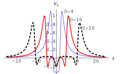
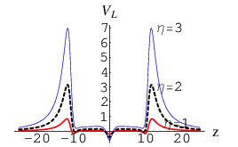
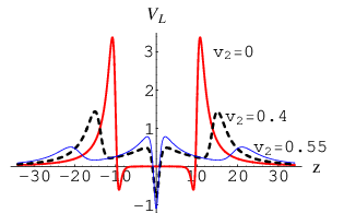
Here, in order to reveal how the parameters affect the potential , we take the three-wall brane () as an example. It is convenient to define the total width of the brane array as , and the spacing of two adjacent sub-branes as . The typical shapes of the three-wall brane are plotted in Fig. 4. There are three inner wells in the potential. As shown in Fig. 4(a), the width of the potential well increases with the parameter , but the depth of the potential well decreases with it. As shown in Fig. 4(b), the depth of the potential well increases with the coupling constant . Moreover, if we fix but leave free, then as shown in Fig. 4(c), it is interesting to see that the potential barriers will decrease with . Especially, for the center inner potential well vanishes since the brane array reduces to a two-wall brane in this case.
As there are many sub-branes in brane array, it is natural to specify where the fermion zero mode is localized. From Eqs. (21) and (31), we have
| (44) |
Figure 5 shows and in physical coordinate for the cases of two-, three-, and four-walls, respectively. It tells us that when there are many sub-branes, the fermion zero mode is localized between the two outermost sub-branes, whose locations are determined by the parameters and . Moreover, every sub-brane will cause an inflection point in the overall shapes of fermion zero mode , such as, there are two inflection points in Fig. 5(a), there are three inflection points in Fig. 5(b), and there are four inflection points in Fig. 5(c), respectively. And the positions of the inflection points are just the centers of sub-branes.


Furthermore, we plot the left-chiral massless fermion with respect to different values of coupling constant for the case of two sub-branes () in Fig. 6. It shows that, as expected, the wave function is more concentrated as increase of the Yukawa interaction strength.

4 Resonances of massive fermions
The continuous massive modes are unbounded and will propagate along the extra dimension. However, as shown in Fig. 4, since the existence of potential barriers, there could be some modes with proper eigenvalues that can stay on the brane for a long time before escaping into the extra dimension. These fermions are called quasi-localized or resonant fermions. In Ref. [48], the influences of some parameters on the resonant fermions on two symmetric and asymmetric sub-branes are analyzed. Here, we focus on studying the property of resonant mass spectra in the brane array.
Following the relative probability method presented in Ref. [49, 50], we calculate the probability of the continuous massive modes in the brane array. In order to numerically solve the solutions of the KK modes in Eqs. (28) and (29), we impose two kinds of boundary conditions, i.e.,
Since the massive modes can not be normalized, it is useful to introduce the relative probability defined as the ratio of probability in interval to the probability in interval , with the coordinate referring to the maximum of the potential [49], namely,
| (48) |
where represents the probability for finding the massive KK mode at the position along the extra dimension. Via scanning the relative probability for different mass, those peaks of the curve indicate the fermion resonant states. Note that the KK modes with will be approximately plane waves and their solutions are or , so the corresponding relative probabilities trends to . Their lifetime can be estimated by , with the width of the half height of the resonant.
4.1 Number of resonant fermions
Since and are partner potentials, we focus on the resonant KK modes of left-chiral fermions here, and the resonant masses of right-chiral fermions are equal to that of left-chiral fermions. Here, we investigate the effects of some factors on the relative probability , namely, the Yukawa coupling constant , the amplitude parameters of the scalar fields, the spacing between the two adjacent sub-branes, the total width of the brane array, and the number of the sub-branes.
Here, in order to investigate the effects of the amplitude parameters and the Yukawa coupling constant on the number of the resonant KK modes, as an example, we set the number of sub-branes as three, and fix the amplitude parameters of outer sub-branes as but leave of middle brane as a variable.


a) The effect of . The curves for number of the resonances versus coupling coupling are shown in Fig. 7, where we have set the width of the brane array to be in Fig. 7(a) and in Fig. 7(b). It is clear that the number of the resonant KK modes increases with the Yukawa coupling constant . This is because the height of potential well increases with the coupling constant as shown in Fig. 4(b). So there are more and more massive resonant modes by strengthening the Yukawa interaction, and this is a well-known result revealed in previous literatures.
b) The effect of . The figure 7(b) shows that the resonance number decreases with the amplitude parameter . This is due to the fact that the height of potential barriers will decrease with , as shown in Fig. 4(c).
c) The effect of . By comparing Fig. 7(a) with Fig. 7(b), it can be concluded that the number of the resonant KK modes increases with the total width of the brane array. This can be understood from the fact that the width of the potential well is proportional to the total width of the brane array, and the broader potential well is, the more resonant KK modes are produced.
If the parameter vanishes, the middle sub-brane disappears, so the curves referring to a null correspond to a two sub-brane system. It indicates that the number of the sub-branes will affect the resonance number. So next we analyze this effect in detail. It is note that one can increase the numbers of the sub-banes with a fixed total width of the brane array, or with a fixed brane spacing . However, since the width of the potential well is approximate to the width of the brane array, if one increases the brane array with a fixed brane spacing , the width and depth of potential well will change both. Therefore, we investigate the effect of simply with a fixed total width .
d) The effect of with fixed total width . We fix the total width , increase the coupling constant from to and change the number of the sub-branes, the brane spacing reads . The effective potential well of the brane array and the relationship of the resonance number with the coupling constant for different values of and fixed is plotted in Fig. 8. Obviously, the resonance number increases with the coupling constant , no matter how much the number of sub-branes is, but decreases when the number of the sub-branes increases (see Fig. 8). This is because the depth of potential well decreases with the number as shown in Fig. 8.


4.2 Mass spectrum of resonant fermions
In order to investigate the properties of the fermion resonant mass spectra on the brane array, we have to input the number of the sub-branes. However, we found the properties are nothing new in models of one and two sub-branes, but there are some novel properties emerging from three or four sub-branes system.


Firstly, we focus on a symmetric four sub-brane model, with the parameters are set to be and . The corresponding effective potential and relative probability are shown in Fig. 9. Any peak in the curves of relative probability refers to a resonant state. The mass spectrum of the resonant states read from Fig. 9 is listed in Tab. 1. It is interesting that there are three resonant states with the masses {0.7472, 0.9755, 1.1897} in both parities. Therefore, the resonant states are doubly-degenerate for the three masses. To the best of our knowledge, this does not happen for the cases of one and two sub-branes, where all the resonant states are non-degenerate and possess either odd-parity or even-parity.
| parity | |||||
| both | |||||
| both | |||||
| odd | |||||
| both | |||||
| even | |||||
| odd |
It is well-known that all the bound states of one-dimensional Schrödinger equation with an even potential must be either odd or even parity. In our case, there is only one non-degenerate massless bound state with even-parity for either left-chiral or right-chiral fermions. For the unbounded states, due to the potential asymptotically vanishing far to the left and far to the right, there are two solutions for each eigenvalue , and the two solutions can be written as one odd and one even functions under the reflection of extra dimension coordinate. So the mass spectrum of massive fermions is continuous and doubly-degenerate. However, by imposing either kind of boundary conditions in Eq. (4), one picks up either odd or even eigenfunctions. Then the condition of being resonance picks up some eigenvalues and leads the resonant mass spectrum being discrete. Generally, if one eigenfunction with a certain parity (either odd or even) possess a low transmission coefficient through a potential barriers with certain mass (or sharply peaked at the curves of relative probability ), the other degenerate eigenfunction with the opposite parity can not possess a low transmission simultaneously. So generally, the resonant states are non-degenerate. This is just the case in one and two sub-brane systems.


However, for the case of four sub-brane system, there are four peaks in the effective potential as is shown in Fig. 9. Comparing with the effective potential of two sub-brane system shown in Fig. 4(c) with , it is clear that there are two additional shallower potential wells on the two shoulders of potential barriers, where bottom of the wells is and top is . The Fig. 9 shows that the eigenvalues {0.7472, 0.9755, 1.1897} of the three resonant states are almost located in the range (0.62746, 1.1541) of the shoulder potential wells. Therefore, it implies that the three doubly-degenerate states may be closely related to the two shoulder potential wells. And this can be verified from the wave functions presented in Fig. 10, where the odd and even wave functions for eigenvalue are plotted in Figs. 10(a) and 10(b) respectively, the odd and even wave functions for in Figs. 10(c) and 10(d) respectively, and the old and even wave function for in Figs. 10(f) and 10(g) respectively. By ascertaining the coordinate ranges of those peaks, it is clear that all the resonant states are quasi-localized in the shoulder potential wells. Specifically, as shown in Figs. 10(a) and 10(b), since the peak of wave functions has no nodes locally in the shoulder potential wells, they are the first resonant state of the shoulder wells. Similarly, Figs. 10(c) and 10(d) indicate that the modes is the second resonant state with one node locally in the shoulder wells, and Figs. 10(f) and 10(g) indicate the modes are the third resonant state with two nodes locally in the shoulder wells. Finally, an even solution is equipped by a symmetric combination of the resonant states of two shoulder wells, and an odd solution by an antisymmetric combination of the resonant states.
However, as illustrated in Figs. 10(e) and 10(h), the non-degenerate modes are manifest quasi-localized in the center potential well. Here, it is note that since the modes in Figs. 10(e) and 10(h) have three and four nodes, respectively. Therefore, there is an even non-degenerate resonance with two nodes and an odd non-degenerate resonance with one node missing in Fig. 9. This is due to their resonant widths are too narrow to be picked out by the precision we used. Further, since the center well is much deeper than the two shoulder wells, the lifetimes of resonances in the center well are much longer than that in the shoulder wells. This is exactly the case presented in table 1, where the lifetimes of non-degenerate resonances are much longer than that of their adjacent degenerate resonances, and it can also be seen clearly from Figs. 9(a) and 9(b), where the non-degenerate resonant modes with eigenvalues and appear as much sharper peaks than the adjacent degenerate resonances in the curves of relative probability.


For the case of three sub-brane system, if there appears two shoulder potential wells, such as the case shown in Fig. 11, it may also exist doubly-degenerate quasi-localized resonant states (see Fig. 11). The corresponding resonant mass spectrum, widths and life times are shown in Tab. 2. As shown in Fig. 11, all the four resonant states are degenerate. On the other hand, it is clear that all the resonances are quasi-localized in the shoulder potential wells by observing the wave functions illustrated in Fig. 12. This is possibly because the central potential well is too narrow to support a resonance. So in this case, the lifetime of the resonances declines monotonously as resonant mass increases. This is different from the case of four sub-brane system, where there are both states localized in central well and shoulder wells.
| parity | |||||
|---|---|---|---|---|---|
| both | |||||
| both | |||||
| both | |||||
| both |


These new properties emerge in the cases of three and four sub-branes, and there is no doubt that it will be more complicated in the cases of more sub-branes. Such as the cases of five and six sub-branes illustrated in Fig. 13, there could be more shoulder potential wells, so there are more series of degenerate resonant modes. Especially, by comparing their potential shapes, we can conclude that the properties of even sub-brane systems are more similar to that of four sub-branes, and the properties of odd sub-brane systems are more similar to that of three sub-branes.
Further, for the usual single-wall braneworld model (simply fixing ), the mass splitting of resonant fermions is proportional to the parameter with mass-dimension one, whose inverse is proportional to brane thickness. Because there is no more mechanism to provide a new mass scale, the parameter is usually set to be the five-dimensional fundamental scale, which is equal to the four-dimensional Planck mass. So it is hopeless to probe the signal of these resonant fermions. However, by including multi sub-branes in the brane array, the resonant fermions are quasi-localized between the whole sub-branes, the mass splitting is related to inverse of the total width of brane array , i.e., proportional to the new mass scale . By including more and more sub-branes, would reduce to a lower and lower mass scale, such as a few TeV. So this novel phenomenon emerging in brane array could be potentially interesting in phenomenology.


5 Conclusions
In this work, we constructed the multi-wall braneworld model with an arbitrary number of bulk scalar fields, and gave two analytic solutions by imposing the polynomial superpotential and modified sine-Gordon superpotential, respectively. Then, for the massless fermion, we studied its localization property on the brane array and came to the conclusion that the massless fermion is localized between the two outermost sub-branes. For the massive resonant fermions, we investigated the effects of some parameters on the number of resonances. We found that the number of resonances increases with the coupling constant and the total width of the brane array, but decreases with the amplitude parameter of the middle sub-brane. Moreover, if we fix the total width , the number of resonances decreases with the number of the sub-branes, while if we fix the brane spacing , the dependency between the number of resonances and the number of the sub-branes is not simply monotonous. Finally, we discussed the mass spectrum of resonant fermions. It is significant that there are doubly-degenerate resonant modes for the cases of three and four sub-brane systems with some sets of parameter values. However, this does not happen for the cases of one and two sub-branes, where all the resonant states are non-degenerate. Besides, the non-degenerate resonant modes appear as much sharper peaks than the adjacent degenerate resonant modes in the curves of relative probability. By setting the mass scale not to be far above TeV, the novel phenomenon emerging in brane array could be potentially interesting in phenomenology, which is left for our future consideration.
References
References
- [1] N. Arkani-Hamed, S. Dimopoulos, and G. R. Dvali, The hierarchy problem and new dimensions at a millimeter, Phys. Lett. B 429 (1998) 263, [arXiv:hep-ph/9803315].
- [2] N. Arkani-Hamed, S. Dimopoulos, N. Kaloper, and R. Sundrum, A small cosmological constant from a large extra dimension, Phys. Lett. B 480 (2000) 193, [arXiv:hep-th/0001197].
- [3] L. Randall and R. Sundrum, A large mass hierarchy from a small extra dimension, Phys. Rev. Lett. 83 (1999) 3370, [arXiv:hep-ph/9905221].
- [4] L. Randall and R. Sundrum, An alternative to compactification, Phys. Rev. Lett. 83 (1999) 4690, [arXiv:hep-th/9906064].
- [5] O. DeWolfe, D. Z. Freedman, S. S. Gubser, and A. Karch, Modeling the fifth dimension with scalars and gravity, Phys. Rev. D 62 (2000) 046008, [arXiv:hep-th/9909134].
- [6] M. Gremm, Four-dimensional gravity on a thick domain wall, Phys. Lett. B 478 (2000) 434, [arXiv: hep-th/9912060].
- [7] M. Gremm, Thick domain walls and singular spaces, Phys. Rev. D 62 (2000) 044017, [arXiv:hep-th/0002040].
- [8] C. Csaki, J. Erlich, T. J. Hollowood, and Y. Shirman, Universal aspects of gravity localized on thick branes, Nucl. Phys. B 581 (2000) 309, [arXiv:hep-th/0001033].
- [9] C. Bogdanos, A. Dimitriadis, and K. Tamvakis, Brane models with a ricci-coupled scalar field, Phys. Rev. D 74 (2006) 045003, [arXiv:hep-th/0604182].
- [10] F.-W. Chen, B.-M. Gu, H. Guo, and Y.-X. Liu, Stability of braneworlds with non-minimally coupled multi-scalar fields, Eur. Phys. J. C 78 (2018) 131, [arXiv:1702.03497].
- [11] Y.-X. Liu, F.-W. Chen, H. Guo, and X.-N. Zhou, Non-minimal coupling branes, JHEP 05 (2012) 108, [arXiv:1205.0210].
- [12] R. Koley and S. Kar, Bulk phantom fields, increasing warp factors and fermion localisation, Mod. Phys. Lett. A 20 (2005) 363, [arXiv:hep-th/0407159].
- [13] D. Bazeia, A. R. Gomes, L. Losano, and R. Menezes, Braneworld models of scalar fields with generalized dynamics, Phys. Lett. B 671 (2009) 402, [arXiv:0808.1815].
- [14] S. Pal and S. Kar, De sitter branes with a bulk scalar, Gen. Rel. Grav. 41 (2009) 1165, [arXiv:hep-th/0701266].
- [15] J. Wang, W.-D. Guo, Z.-C. Lin, and Y.-X. Liu, Braneworld in Gravity Theory with Noncanonical Scalar Matter Field, Phys. Rev. D 98 (2018) 084046, [arXiv:1808.00771].
- [16] Z.-Q. Cui, Y.-X. Liu, B.-M. Gu, and L. Zhao, Linear stability of thick branes: tensor perturbations, JHEP 11 (2018) 083, [arXiv:1802.01454].
- [17] V. I. Afonso, D. Bazeia, R. Menezes, and A.Yu. Petrov, -Brane, Phys. Lett. B 658 (2007) 71, [arXiv:0710.3790].
- [18] V. Dzhunushaliev, V. Folomeev, B. Kleihaus, and J. Kunz, Some thick brane solutions in -gravity, JHEP 04 (2010) 130, [arXiv:0912.2812].
- [19] B.-M. Gu, Y.-X. Liu, Y. Zhong, Stable Palatini braneworld, Phys. Rev. D 98 (2018) 024027, [arXiv:1804.00271].
- [20] D. Bazeia, A. Lobao, R. Menezes, A. Y. Petrov, and A. da Silva, Braneworld solutions for models with non-constant curvature, Phys. Lett. B 729 (2014) 127, [arXiv:1311.6294].
- [21] H. Yu, Y. Zhong, B.-M. Gu, and Y.-X. Liu, Gravitational resonances on -brane, Eur. Phys. J. C 76 (2016) 195, [arXiv:1506.06458].
- [22] Y. Zhong, Y.-X. Liu, Pure geometric thick -branes: stability and localization of gravity, Eur. Phys. J. C 76 (2016) 321, [arXiv:1507.00630].
- [23] J. Yang, Y.-L. Li, Y. Zhong, and Y. Li, Thick brane split caused by spacetime torsion, Phys. Rev. D 85 (2012) 084033, [arXiv:1202.0129].
- [24] R. Menezes, First order formalism for thick branes in modified teleparallel gravity, Phys. Rev. D 89 (2014) 125007, [arXiv:1403.5587].
- [25] K. Yang, W.-D. Guo, Z.-C. Lin, and Y.-X. Liu, Domain wall brane in a reduced Born-Infeld- theory, Phys. Lett. B 782 (2018) 170, [arXiv:1709.01047].
- [26] W.-D. Guo, Q.-M. Fu, Y.-P. Zhang, and Y.-X. Liu, Tensor perturbations of f(T)-branes, Phys. Rev. D 93 (2016) 044002, [arXiv:1511.07143].
- [27] B.-M. Gu, Y.-P. Zhang, H. Yu, and Y.-X. Liu, Full linear perturbations and localization of gravity on brane, Eur. Phys. J. C 77 (2017) 115, [arXiv:1606.07169].
- [28] O. Arias, R. Cardenas, and I. Quiros, Thick brane worlds arising from pure geometry, Nucl. Phys. B 643 (2002) 187, [arXiv:hep-th/0202130].
- [29] N. Barbosa-Cendejas and A. Herrera-Aguilar, 4d gravity localized in non -symmetric thick branes, JHEP 10 (2005) 101, [arXiv:hep-th/0511050].
- [30] Y.-X. Liu, K. Yang, H. Guo, and Y. Zhong, Domain wall brane in eddington inspired born-infeld gravity, Phys. Rev. D 85 (2012) 124053, [arXiv:1203.2349].
- [31] Q.-M. Fu, L. Zhao, K. Yang, B.-M. Gu, and Y.-X. Liu, Stability and (quasi)localization of gravitational fluctuations in an eddington-inspired born-infeld brane system, Phys. Rev. D 90 (2014) 104007, [arXiv:1407.6107].
- [32] A. Kehagias and K. Tamvakis, Localized gravitons, gauge bosons and chiral fermions in smooth spaces generated by a bounce, Phys. Lett. B 504 (2001) 38, [arXiv:hep-th/0010112].
- [33] D. Bazeia, L. Losano, and C. Wotzasek, Domain walls in three field models, Phys. Rev. D 66 (2002) 105025, [arXiv:hep-th/0206031].
- [34] D. Bazeia and A. R. Gomes, Bloch brane, JHEP 05 (2004) 012, [arXiv:hep-th/0403141].
- [35] M. O. Tahim, W. T. Cruz, and C. A. S. Almeida, Tensor gauge field localization in branes, Phys. Rev. D 79 (2009) 085022, [arXiv:0808.2199].
- [36] D. Bazeia, A. Lobao, L. Losano, and R. Menezes, First-order formalism for flat branes in generalized n-field models, Phys. Rev. D 88 (2013) 045001, [arXiv:1306.2618].
- [37] M. Peyrard and M. Kruskal, Kink dynamics in the highly discrete sine-gordon system, Physica D 14 (1984) 88.
- [38] A. Campos, Critical phenomena of thick branes in warped spacetimes, Phys. Rev. Lett. 88 (2002) 141602, [arXiv:hep-th/0111207].
- [39] A. E. R. Chumbes, A. E. O. Vasquez, and M. B. Hott, Fermion localization on a split brane, Phys. Rev. D 83 (2011) 105010.
- [40] G. P. de Brito, R. A. C. Correa, and A. de Souza Dutra, Analytical multikinks in smooth potentials, Phys. Rev. D 89 (2014) 065039, [arXiv:1403.2951].
- [41] V. Dzhunushaliev, V. Folomeev, and M. Minamitsuji, Thick brane solutions, Rept. Prog. Phys. 73 (2010) 066901, [arXiv:0904.1775].
- [42] Y.-X. Liu, Introduction to Extra Dimensions and Thick Braneworlds, Memorial Volume for Yi-Shi Duan, Chapter 8 (2018) 211, [arXiv:1707.08541].
- [43] A. de Souza Dutra, A. C. A. de Faria, Jr., and M. Hott, Degenerate and critical Bloch branes, Phys. Rev. D 78 (2008) 043526, [arXiv:0807.0586].
- [44] A. de Souza Dutra, G. P. de Brito, and J. M. Hoff da Silva, Method for obtaining thick brane models, Phys. Rev. D 91 (2015) 086016, [arXiv:1412.5543].
- [45] A. Farokhtabar and A. Tofighi, Localization of Massive and Massless Fermions on Two-Field Branes, Adv. High Energy Phys. 2017 (2017) 3926286, [arXiv:1610.00899].
- [46] V. Afonso, D. Bazeia, and L. Losano, First-order formalism for bent brane, Phys. Lett. B 634 (2006) 526, [arXiv: hep-th/0601069].
- [47] S. Randjbar-Daemi and M. E. Shaposhnikov, Fermion zero modes on brane worlds, Phys. Lett. B 492 (2000) 361, [hep-th/0008079].
- [48] Q.-Y. Xie, J. Yang, and L. Zhao, Resonance Mass Spectra of Gravity and Fermion on Bloch Branes, Phys. Rev. D 88 (2013) 105014, [arXiv:1310.4585].
- [49] C. A. S. Almeida, M. M. Ferreira Jr., A. R. Gomes, and R. Casana, Fermion localization and resonances on two-field thick branes, Phys. Rev. D 79 (2009) 125022, [arXiv:0901.3543].
- [50] Y.-X. Liu, J. Yang, Z.-H. Zhao, C.-E. Fu, and Y.-S. Duan, Fermion localization and resonances on a de sitter thick brane, Phys. Rev. D 80 (2009) 065019, [arXiv:0904.1785].