跳到论文正文
W Papers独立论文阅读器 arXiv:1901.11221 论文正文 计算阅读时间 · 0%
引用这篇论文根据当前论文元数据生成,正式投稿前建议核对。


License: arXiv.org perpetual non-exclusive license
arXiv:1901.11221v1 [stat.ML] 31 Jan 2019

Contextual Multi-armed Bandit Algorithm for Semiparametric Reward Model

Gi-Soo Kim Affiliation: Department of Statistics Affiliation: Seoul National University Affiliation: Seoul, Korea Email: gisoo1989@snu.ac.kr    Myunghee Cho Paik* Affiliation: Department of Statistics Affiliation: Seoul National University Affiliation: Seoul, Korea Email: myungheechopaik@snu.ac.kr
Abstract

Contextual multi-armed bandit (MAB) algorithms have been shown promising for maximizing cumulative rewards in sequential decision tasks such as news article recommendation systems, web page ad placement algorithms, and mobile health. However, most of the proposed contextual MAB algorithms assume linear relationships between the reward and the context of the action. This paper proposes a new contextual MAB algorithm for a relaxed, semiparametric reward model that supports nonstationarity. The proposed method is less restrictive, easier to implement and faster than two alternative algorithms that consider the same model, while achieving a tight regret upper bound. We prove that the high-probability upper bound of the regret incurred by the proposed algorithm has the same order as the Thompson sampling algorithm for linear reward models. The proposed and existing algorithms are evaluated via simulation and also applied to Yahoo! news article recommendation log data.

Keywords Contextual multi-armed bandit algorithm ⋅\cdot Thompson sampling ⋅\cdot Semiparametric model

1 Introduction

The multi-armed bandit (MAB) problem (Robbins, 1952) formulates the sequential decision problem in which a learner must choose an action among several actions given by the environment at each step so as to maximize the cumulative rewards. The actions are often described as the arms of a bandit slot machine with multiple arms. By choosing an action or pulling an arm, the learner receives possibly different rewards. By repeating the process of pulling arms and receiving rewards, the learner accumulates information about the reward compensation mechanism, learns from it, and chooses the arm close to optimal as time elapses. Application areas include the mobile healthcare system (Tewari and Murphy, 2017), web page ad placement algorithms (Langford et al., 2008), news article placement algorithms (Li et al., 2010), revenue management (Ferreira et al., 2018), marketing (Schwartz et al., 2017), and recommendation systems (Kawale et al., 2015).

For example, the Yahoo! web system uses a news article recommendation algorithm to select one article among a large pool of available articles and displays it on the Featured tab of the web page every time a user visits. The user clicks the article if he or she is interested in the contents. The goal of the algorithm is to maximize the cumulative number of user clicks. After each visit, the algorithm reinforces its article selection strategy based on the past user click feedback. In this setting, available articles correspond to different actions and the user click corresponds to a reward. The challenging part of the MAB problem is that the reward of the action that the learner has not previously chosen is forever unknown, i.e., whether the user would have clicked or not remains missing for the article that is not chosen. Therefore, the learner should balance between “exploitation", selecting the best action based on information accumulated so far, and “exploration", choosing an action that will assist in future choices, although it does not seem to be the best option at the moment.

The MAB problem was first theoretically analyzed by Lai and Robbins, 1985. The algorithms widely used in mobile healthcare systems or news article placement algorithms are of a more extended form, called contextual MAB algorithms. A contextual MAB algorithm enables at each selection step the use of side information, called context, about each action given in the form of finite-dimensional covariates. For example, in the news article recommendation, information on the visiting user as well as the articles are given in the form of a context vector. In 2010, the Yahoo! team (Li et al., 2010) proposed a contextual MAB algorithm that achieved a 12.5% click lift compared to a context-free MAB algorithm. Nonetheless, the method of Li et al., 2010 and other existing algorithms rely on rather strong assumptions on the distribution of rewards. In particular, most of the existing algorithms assume that the expectation of the reward of a particular action has a time-invariant linear relationship with the context vector. This assumption can be restrictive in real world settings where the rewards typically vary with time.

In this paper, we propose a novel contextual MAB algorithm which works well under a relaxed assumption on the distribution of rewards. The relaxed nature of the assumption involves nonstationarity of the reward via an additive intercept term to the original time-invariant linear term. This intercept term changes with time but does not depend on the action. We propose a consistent estimation of the regression parameter in the linear term by centering the context vectors with weights. Using new martingale inequalities, we prove that the high probability upper bound of the total regret incurred by the proposed algorithm has the same order as the regret bound achieved by the Thompson sampling algorithm which is developed under a more restrictive linear assumption.

Greenewald et al., 2017 and Krishnamurthy et al., 2018 suggested algorithms under the same nonstationary assumption we considered. The performance of the method by Greenewald et al., 2017 is guaranteed under restrictive conditions on the action choice probabilities. The method by Krishnamurthy et al., 2018 takes an action-elimination approach which is computationally heavy as it requires O⁡(N2)O(N^{2}) computations at each iteration where NN denotes the number of arms. Moreover in Krishnamurthy et al., 2018, the action selection distribution is not given explicitly when N>2N>2. Our method improves on these previous results in that it does not restrict action choice probabilities, requires O⁡(N)O(N) computations, and explicitly provides the action selection distribution for every NN. Furthermore, the proposed estimator for the regression parameter achieves the same convergence rate as the estimator for linear reward models.

As a summary, our main contributions are:

  • •

    We propose a new MAB algorithm for the nonstationary semiparametric reward model. The proposed method is less restrictive, easier to implement and computationally faster than previous works.

  • •

    We prove that the high-probability upper bound of the regret for the proposed method is of the same order as the Thompson Sampling algorithm for linear reward models.

  • •

    We propose a new estimator for the regression parameter without requiring an extra tuning parameter and prove that it converges to the true parameter faster than existing estimators.

  • •

    Simulation studies show that in most cases, the cumulative reward of the proposed method increases faster than existing methods which assume the same nonstationary reward model. Application to Yahoo! news article recommendation log data shows that the proposed method increases the user click rate compared to the algorithms that assume a stationary reward model.

2 Preliminaries

In this section, we describe the problem settings and notations. As a preliminary, we also present a review of contextual bandit methods for the comparison purpose with the proposed method given in Section 4.

In the MAB setting, the learner is repeatedly faced with NN alternative actions where at time tt, the ii-th arm (i=1,⋯,Ni=1,\cdots,N) yields a random reward ri​(t)r_{i}(t) with unknown mean θi​(t)\theta_{i}(t). In the contextual MAB problem, we assume that there is a finite-dimensional context vector bi​(t)∈ℝdb_{i}(t)\in\mathbb{R}^{d} associated with each arm ii at time tt and that the mean of ri​(t)r_{i}(t) depends on bi​(t)b_{i}(t), i.e., θi​(t)=θt​(bi​(t)),\theta_{i}(t)=\theta_{t}(b_{i}(t)), where θt​(⋅)\theta_{t}(\cdot) is an arbitrary function. Among the NN arms, the learner pulls one arm a⁡(t)a(t), and observes reward ra⁡(t)​(t)r_{a(t)}(t). The optimal arm at time tt is a∗​(t):=argmax1≤i≤N​{θt​(bi​(t))}a^{*}(t):=\underset{1\leq i\leq N}{\mathrm{argmax}}\{\theta_{t}(b_{i}(t))\}. Let r​e​g​r​e​t​(t)regret(t) be the difference between the expected reward of the optimal arm and the expected reward of the arm chosen by the learner at time tt, i.e.,

r​e​g​r​e​t​(t)\displaystyle regret(t) =𝔼⁡(ra∗​(t)​(t)−ra⁡(t)​(t)|{bi​(t)}i=1N,a⁡(t))\displaystyle=\mathbb{E}\big(r_{a^{*}(t)}(t)-r_{a(t)}(t)~\big|~\{b_{i}(t)\}_{i=1}^{N},a(t)~\big)
=θt​(ba∗​(t)​(t))−θt​(ba⁡(t)​(t)).\displaystyle=\theta_{t}(b_{a^{*}(t)}(t))-\theta_{t}(b_{a(t)}(t)).

Then, the goal of the learner is to minimize the sum of regrets over TT steps, R⁡(T):=∑t=1Tr​e​g​r​e​t​(t).R(T):=\sum_{t=1}^{T}regret(t).

Linear contextual MAB problems specifically assume that θt​(bi​(t))\theta_{t}(b_{i}(t)) is linear in bi​(t)b_{i}(t),

θt(bi(t))=bi(t)Tμ,i=1,⋯,N,\displaystyle\theta_{t}(b_{i}(t))=b_{i}(t)^{T}\mu,~~~i=1,\cdots,N, (1)

where μ∈ℝd\mu\in\mathbb{R}^{d} is unknown. For the linear contextual MAB problem, Dani et al., 2008 proved a lower bound of order Ω⁡(d​T)\Omega(d\sqrt{T}) for the regret R⁡(T)R(T) when NN is allowed to be infinite. When NN is finite and d2≤Td^{2}\leq T , Chu et al., 2011 showed a lower bound of Ω⁡(d​T)\Omega(\sqrt{dT}).

Auer, 2002, Li et al., 2010 and Chu et al., 2011 proposed an upper confidence bound (UCB) algorithm for the linear contextual MAB problem. The algorithm selects the arm which has the highest UCB of the reward. Since the UCB reflects the current estimate of the reward as well as its uncertainty, the algorithm naturally balances between exploitation and exploration. The success of the UCB algorithm hinges on a valid upper confidence bound Ui​(t)U_{i}(t) of the ii-th arm’s reward, bi​(t)T​μb_{i}(t)^{T}\mu. Li et al., 2010 and Chu et al., 2011 proposed

Ui​(t)=bi​(t)T​μ^​(t)+α​st,i,U_{i}(t)=b_{i}(t)^{T}\hat{\mu}(t)+\alpha s_{t,i},

where μ^​(t)\hat{\mu}(t) is the regression estimator of μ\mu at time tt,

μ^​(t)=B​(t)−1​∑τ=1t−1ba⁡(τ)​(τ)​ra⁡(τ)​(τ),\displaystyle\hat{\mu}(t)=B(t)^{-1}\sum_{\tau=1}^{t-1}b_{a(\tau)}(\tau)r_{a(\tau)}(\tau), (2)

B⁡(t)=Id+∑τ=1t−1ba⁡(τ)​(τ)​ba⁡(τ)​(τ)TB(t)=I_{d}+\sum_{\tau=1}^{t-1}b_{a(\tau)}(\tau)b_{a(\tau)}(\tau)^{T} and st,i=bi​(t)T​B​(t)−1​bi​(t).s_{t,i}=\sqrt{b_{i}(t)^{T}B(t)^{-1}b_{i}(t)}.

Under additional assumptions that the error ηi​(t):=ri​(t)−𝔼⁡(ri​(t)|bi​(t))=ri​(t)−bi​(t)T​μ\eta_{i}(t):=r_{i}(t)-\mathbb{E}(r_{i}(t)|b_{i}(t))=r_{i}(t)-b_{i}(t)^{T}\mu is RR-sub-Gaussian for some R>0R>0 and that the L2L_{2}-norms of bi​(t)b_{i}(t) and μ\mu are bounded by 11, Abbasi-Yadkori et al., 2011 proved that if we set α=R​3​d​log​(T/δ)+1\alpha=R\sqrt{3d\mathrm{log}({T}/{\delta})}+1, Ui​(t)U_{i}(t) is a (1−δ)(1-\delta)-probability upper bound of bi​(t)T​μb_{i}(t)^{T}\mu for ∀δ∈(0,1)\forall\delta\in(0,1), for all i=1,⋯,Ni=1,\cdots,N and t=1,⋯,Tt=1,\cdots,T. Since the errors ηa⁡(τ)​(τ)\eta_{a(\tau)}(\tau)’s of the observed rewards are intercorrelated, Abbasi-Yadkori et al., 2011 used a concentration inequality for vector-valued martingales to derive a tight α\alpha. Additionally, Abbasi-Yadkori et al., 2011 proved that with probability at least 1−δ1-\delta, the UCB algorithm achieves,

R⁡(T)\displaystyle R(T) ≤O⁡(d​T​log​(T/δ)​log​(1+T/d)).\displaystyle\leq O\big(d\sqrt{T\mathrm{log}({T}/{\delta})\mathrm{log}(1+{T}/{d})}\big). (3)

The bound (3) matches the lower bound Ω⁡(d​T)\Omega(d\sqrt{T}) for infinite NN by a factor of log⁡(T)\mathrm{log}(T). When NN is finite, (3) is slightly higher than the lower bound Ω⁡(d​T)\Omega(\sqrt{dT}) by a factor of d​log​(T).\sqrt{d}\mathrm{log}(T).

As a randomized version of the UCB algorithm, Thompson sampling (Thompson, 1933) has been widely used as a simple heuristic based on Bayesian ideas. Agrawal and Goyal, 2013 was the first to propose and analyze the Thompson sampling (TS) algorithm for linear contextual MABs.

The heuristic of the algorithm is to randomly pull the arm according to the posterior probability that it is the optimal arm. This can be done by sampling μ~​(t)\tilde{\mu}(t) from the posterior distribution of μ\mu at time tt, and pulling the arm a⁡(t)=argmax1≤i≤N​bi​(t)T​μ~​(t)a(t)=\underset{1\leq i\leq N}{\mathrm{argmax}}~b_{i}(t)^{T}\tilde{\mu}(t). The posterior distribution 𝒩⁡(μ^​(t),v2​B​(t)−1)\mathcal{N}(\hat{\mu}(t),v^{2}B(t)^{-1}) with μ^​(t)\hat{\mu}(t) defined in (2) is easily derived by assuming a gaussian prior 𝒩⁡(0d,v2​Id)\mathcal{N}(0_{d},v^{2}I_{d}) on μ\mu for some v>0v>0 and that ri​(t)r_{i}(t) given μ\mu follows a gaussian distribution 𝒩⁡(bi​(t)T​μ,v2).\mathcal{N}(b_{i}(t)^{T}\mu,v^{2}).

Agrawal and Goyal, 2013 derived the high-probability upper bound of R⁡(T)R(T) for the TS algorithm. This bound does not require the Bayesian framework nor the gaussian assumption for the rewards. Under (1) and RR-sub-gaussianity of the errors, it can be shown that with probability greater than 1−δ,1-\delta,

R⁡(T)\displaystyle R(T) ≤O⁡(d32​T​log​(T​d)​log​(T/δ)​(log⁡(1+T/d)+log⁡(1/δ))).\displaystyle\leq O\big(d^{\frac{3}{2}}\sqrt{T\mathrm{log}(Td)\mathrm{log}(T/\delta)}(\sqrt{\mathrm{log}(1+T/d)}+\sqrt{\mathrm{log}(1/\delta)}~)\big). (4)

The bound (4) matches the bound (3) by a factor of d​log⁡(T)\sqrt{d}\sqrt{\mathrm{log}(T)}, which is the price for randomness. On the other hand, the TS algorithm does not require the for loop in the UCB algorithm to compute the st,i′​ss_{t,i}^{\prime}s for each arm ii.

Unlike aforementioned linear contextual MABs, adversarial contextual MABs do not impose any assumption on the functional form of θt​(⋅)\theta_{t}(\cdot). Hence, the distribution of ri​(t)r_{i}(t) is allowed to change over time, and it can also change adaptively depending on the history. In fact, we assume that an unknown adversary controls the value of ri​(t)r_{i}(t) in a way that hampers the learner. In this more relaxed setting though, it is hard to achieve low r​e​g​r​e​t​(t)regret(t) with respect to the best choice ra∗​(t)​(t)r_{a^{*}(t)}(t). Instead, the learner competes with a predefined, finite set of KK policies and the regret is defined with respect to the best policy in that set.

The EXP4.P algorithm proposed by Beygelzimer et al., 2011 achieves O⁡(T​N​log​(K/δ))O(\sqrt{TN\mathrm{log}({K}/{\delta})}) regret upper bound. However, for the new notion of regret to be close to the more conservative definition, KK should be as large as possible so as to contain the optimal policy which chooses a∗​(t)a^{*}(t) for every tt, resulting in larger regret. Therefore, when a simple parametric or semiparametric assumption is not considered so farfetched, algorithms that exploit this structure can lead to higher rewards.

3 Semiparametric contextual MAB

Greenewald et al., 2017 and Krishnamurthy et al., 2018 considered a middle ground between simple linear contextual MABs and complex adversarial MABs: a semiparametric contextual MAB. In this section, we formally present the semiparametric contextual MAB problem and related works.

3.1 Semiparametric additive reward model

Hereinafter, we define ℋt−1\mathcal{H}_{t-1} as the history until time t−1t-1, i.e., ℋt−1={a⁡(τ),ra⁡(τ)​(τ),{bi​(τ)}i=1N,τ=1,⋯,t−1},\mathcal{H}_{t-1}=\{a(\tau),r_{a(\tau)}(\tau),\{b_{i}(\tau)\}_{i=1}^{N},\tau=1,\cdots,t-1\}, and the filtration ℱt−1\mathcal{F}_{t-1} as the union of ℋt−1\mathcal{H}_{t-1} and the contexts at time tt, i.e., ℱt−1={ℋt−1,{bi​(t)}i=1N}\mathcal{F}_{t-1}=\{\mathcal{H}_{t-1},\{b_{i}(t)\}_{i=1}^{N}\} for t=1,⋯,T.t=1,\cdots,T. Given ℱt−1\mathcal{F}_{t-1}, we assume that the expectation of the reward ri​(t)r_{i}(t) can be decomposed into a time-invariant, linear component depending on action (bi​(t)T​μ)(b_{i}(t)^{T}\mu) and a nonparametric component depending on time and possibly on ℱt−1\mathcal{F}_{t-1}, but not on the action (ν⁡(t)\nu(t)):

𝔼⁡(ri​(t)|ℱt−1)=ν⁡(t)+bi​(t)T​μ.\displaystyle\mathbb{E}(r_{i}(t)|\mathcal{F}_{t-1})=\nu(t)+b_{i}(t)^{T}\mu. (5)

In (5), we do not impose any distributional assumption on ν⁡(t)\nu(t) except that it is bounded, |ν⁡(t)|≤1|\nu(t)|\leq 1. If ν⁡(t)=0\nu(t)=0, the problem is just a linear contextual MAB problem, whereas if ν⁡(t)\nu(t) depends on the action as well, the reward distribution is completely nonparametric and can be addressed by adversarial MAB algorithms.

In the news article recommendation example, ν⁡(t)\nu(t) can represent the baseline tendency of the user visiting at time tt to click any article in the Featured tab, regardless of the contents of the article. This baseline tendency can change in an unexpected manner, because different users visit at each time and even for the same user, the clicking tendency can change according to the user’s mood or schedule, both of which cannot be captured as contextual information. It is reasonable to assume that given this baseline tendency, the probability that the user clicks an article is linear with respect to context information of the article and the user.

Under (5), we note that the optimal action a∗​(t)a^{*}(t) at time tt does not depend on ν⁡(t)\nu(t) but only on the value of μ\mu, and the regret does not depend on ν⁡(t)\nu(t) either:

r​e​g​r​e​t​(t)=ba∗​(t)​(t)T​μ−ba⁡(t)​(t)T​μ.regret(t)=b_{a^{*}(t)}(t)^{T}\mu-b_{a(t)}(t)^{T}\mu.

However, ν⁡(t)\nu(t) confounds the estimation of μ\mu. The nature of the bandit problem renders the distinction of ν⁡(t)\nu(t) from the linear part especially difficult because only one observation is allowed at each time tt. Moreover, under the partially adversarial model (5), deterministic algorithms such as UCB algorithms turn out to be useless. This is because for deterministic algorithms, a⁡(t)∈ℱt−1a(t)\in\mathcal{F}_{t-1}. Hence, if an adversary sets ν⁡(t)∈ℱt−1\nu(t)\in\mathcal{F}_{t-1} to be ν⁡(t)=−ba⁡(t)​(t)T​μ\nu(t)=-b_{a(t)}(t)^{T}\mu, the observed reward is ra⁡(t)​(t)=ηa⁡(t)​(t)r_{a(t)}(t)=\eta_{a(t)}(t) for all t=1,⋯,Tt=1,\cdots,T, and the algorithm cannot learn μ\mu. Therefore, we should capitalize on the randomness of action choice.

Besides (5), we make the usual assumption that given ℱt−1\mathcal{F}_{t-1}, the error ηi​(t):=ri​(t)−𝔼⁡(ri​(t)|ℱt−1)\eta_{i}(t):=r_{i}(t)-\mathbb{E}(r_{i}(t)|\mathcal{F}_{t-1}) is RR-sub-Gaussian for some R>0R>0, i.e., for every λ∈ℝ,\lambda\in\mathbb{R},

𝔼⁡[exp⁡(λ​ηi​(t))|ℱt−1]≤exp⁡(λ2​R2/2).\displaystyle\mathbb{E}[\mathrm{exp}(\lambda\eta_{i}(t))|\mathcal{F}_{t-1}]\leq\mathrm{exp}({\lambda^{2}R^{2}}/{2}). (6)

Note that this assumption is satisfied whenever ri​(t)∈[ν⁡(t)+bi​(t)T​μ−R,ν⁡(t)+bi​(t)T​μ+R]r_{i}(t)\in[\nu(t)+b_{i}(t)^{T}\mu-R,\nu(t)+b_{i}(t)^{T}\mu+R]. Also without loss of generality, we assume

‖bi​(t)‖2≤1,‖μ‖2≤1,|ν⁡(t)|≤1,\displaystyle||b_{i}(t)||_{2}\leq 1,~||\mu||_{2}\leq 1,~|\nu(t)|\leq 1, (7)

where ||⋅||p||\cdot||_{p} denotes the LpL_{p}-norm.

3.2 Related Work

Greenewald et al., 2017 proposed the action-centered TS algorithm for the new reward model (5). In their settings, they assumed that the first action is the base action, of which the context vector is b1​(t)=0db_{1}(t)=0_{d} for all tt. Hence, the expected reward of the base action is ν⁡(t)\nu(t), which can vary with time and also in a way that depends on the past. Greenewald et al., 2017 followed the basic framework of the randomized, TS algorithm but in two stages. In the first stage, the learner selects one action among the non-base actions in the same way as in TS algorithm using random μ~​(t)\tilde{\mu}(t). Let this action be a¯​(t)\bar{a}(t). In the second stage, the learner chooses once again between a¯​(t)\bar{a}(t) and the base action using the distribution of μ~​(t)\tilde{\mu}(t). This finally chosen action is set as a⁡(t)a(t) and only this action is actually taken. In the second stage, the probability of a​(t)=a¯​(t)a(t)=\bar{a}(t) is computed using the Gaussian distribution of μ~​(t)\tilde{\mu}(t), ℙ⁡(a⁡(t)=a¯​(t)|ℱt−1,a¯​(t))=1−ψ⁡(−ba¯​(t)​(t)T​μ^​(t)v​st,a¯​(t)​(t)),\mathbb{P}(a(t)=\bar{a}(t)|\mathcal{F}_{t-1},\bar{a}(t))=1-\psi\Big(\frac{-b_{\bar{a}(t)}(t)^{T}\hat{\mu}(t)}{vs_{t,\bar{a}(t)}(t)}\Big), where ψ⁡(⋅)\psi(\cdot) is the CDF of the standard Gaussian distribution.

Instead of choosing a​(t)=a¯​(t)a(t)=\bar{a}(t) with this exact probability however, Greenewald et al., 2017 constrained the probability of not choosing the base action to lie in a predefined set [pm​i​n,pm​a​x]⊂[0,1][p_{min},p_{max}]\subset[0,1]. This is to prevent the policy from converging to a determinisitic policy which can be ineffective in the mobile health setting that the authors considered. Hence, the algorithm selects a​(t)=a¯​(t)a(t)=\bar{a}(t) with probability pt=max⁡(pm​i​n,min⁡(1−ψ⁡(−ba¯​(t)​(t)T​μ^​(t)v​st,a¯​(t)​(t)),pm​a​x)).p_{t}=\mathrm{max}\Big(p_{min},~\mathrm{min}\Big(1-\psi\Big(\frac{-b_{\bar{a}(t)}(t)^{T}\hat{\mu}(t)}{vs_{t,\bar{a}(t)}(t)}\Big),~p_{max}\Big)\Big). Under this probability constraint, the definition of the optimal policy and r​e​g​r​e​t​(t)regret(t) changes accordingly. Let a¯∗​(t)=argmax2≤i≤N​bi​(t)T​μ\bar{a}^{*}(t)=\underset{2\leq i\leq N}{\mathrm{argmax}}~b_{i}(t)^{T}\mu. Thus, a¯∗​(t)\bar{a}^{*}(t) is the optimal action among the non-base actions. Then the optimal policy chooses the action a∗​(t)=a¯∗​(t)a^{*}(t)=\bar{a}^{*}(t) with probability π∗​(t):=pm​a​x​I​(ba¯∗​(t)​(t)T​μ>0)+pm​i​n​I​(ba¯∗​(t)​(t)T​μ≤0)\pi^{*}(t):=p_{max}I(b_{\bar{a}^{*}(t)}(t)^{T}\mu>0)+p_{min}I(b_{\bar{a}^{*}(t)}(t)^{T}\mu\leq 0) and a∗​(t)=1a^{*}(t)=1 with probability 1−π∗​(t).1-\pi^{*}(t).

To consistently estimate μ\mu, Greenewald et al., 2017 defined a pseudo-reward, r^a¯​(t)​(t)={I⁡(a⁡(t)=a¯​(t))−pt}​ra⁡(t)​(t).\hat{r}_{\bar{a}(t)}(t)=\{I(a(t)=\bar{a}(t))-p_{t}\}r_{a(t)}(t). An important property of the pseudo-reward is that its conditional expectation does not depend on ν⁡(t)\nu(t). Greenewald et al., 2017 used this pseudo-reward instead of the actual reward ra⁡(t)​(t)r_{a(t)}(t) for estimating μ\mu. They showed that the high probability upper bound of R⁡(T)R(T) for the action-centered TS algorithm matches that of the original TS algorithm for linear reward models, but by a constant factor M=1/{pm​i​n​(1−pm​a​x)}M=1/\{p_{min}(1-p_{max})\}. This factor MM can be large when we do not want to restrict action selection probabilities, i.e., when we want to set either pm​i​n=0p_{min}=0 or pm​a​x=1p_{max}=1.

Krishnamurthy et al., 2018 proposed the BOSE (Bandit Orthogonalized Semiparametric Estimation) algorithm for the semiparametric reward model (5). This algorithm takes an action elimination method adapted from Even-Dar et al., 2006. At each time tt, an action ii is eliminated if there exists another action jj such that (bj​(t)−bi​(t))T​μ^​(t)>ω​(bi​(t)−bj​(t))T​Vt−1​(bi​(t)−bj​(t)),\big(b_{j}(t)-b_{i}(t)\big)^{T}\hat{\mu}(t)>\omega\sqrt{(b_{i}(t)-b_{j}(t))^{T}V_{t}^{-1}(b_{i}(t)-b_{j}(t))}, where ω\omega is a predefined constant, μ^​(t)\hat{\mu}(t) is an estimate of μ\mu, and VtV_{t} is a dd-dimensional matrix. The algorithm then picks up one action randomly among the survivors according to a particular distribution.

For estimating μ\mu, Krishnamurthy et al., 2018 used a centering trick on the context vectors bi​(t)b_{i}(t)’s to cancel out ν⁡(t)\nu(t). They proposed the following estimator for μ\mu:

μ^​(t)=(γ​Id+∑τ=1t−1Xτ​XτT)−1​∑τ=1t−1Xτ​ra⁡(τ)​(τ),\displaystyle\hat{\mu}(t)=\big(\gamma I_{d}+\sum_{\tau=1}^{t-1}X_{\tau}X_{\tau}^{T}\big)^{-1}\sum_{\tau=1}^{t-1}X_{\tau}r_{a(\tau)}(\tau), (8)

where Xτ=ba⁡(τ)​(τ)−𝔼⁡(ba⁡(τ)​(τ)|ℱτ−1)X_{\tau}=b_{a(\tau)}(\tau)-\mathbb{E}(b_{a(\tau)}(\tau)|\mathcal{F}_{\tau-1}) and γ>0\gamma>0. Given ℱτ−1\mathcal{F}_{\tau-1}, we see that 𝔼⁡(Xτ|ℱτ−1)=0d.\mathbb{E}(X_{\tau}|\mathcal{F}_{\tau-1})=0_{d}. Hence, {∑τ=1tXτ}t=1∞\{\sum_{\tau=1}^{t}X_{\tau}\}_{t=1}^{\infty} is a vector martingale process adapted to filtration {ℱt}t=1∞\{\mathcal{F}_{t}\}_{t=1}^{\infty}. Krishnamurthy et al., 2018 derived a (1−δ1-\delta)-probability upper bound for bT​(μ^​(t)−μ)b^{T}(\hat{\mu}(t)-\mu) using a new concentration inequality for self-normalized vector-valued martingales established by de la Peña et al., 2009 and de la Peña et al., 2004.

The BOSE algorithm does not require any constraint on the action choice probabilities but achieves a O⁡(d​T​log​(T/δ))O(d\sqrt{T}\mathrm{log}(T/\delta)) regret bound. This bound matches the best known regret bound (3) for linear reward models. However, the action elimination step requires O⁡(N2)O(N^{2}) computations at each round. Also, the distribution used to select the action should satisfy a specific condition to guarantee the O⁡(d​T​log​(T/δ))O(d\sqrt{T}\mathrm{log}(T/\delta)) regret bound. The authors only show that there exists a distribution to satisfy this condition when N>2N>2. The construction of such distribution is not a trivial matter since it requires to solve a convex program with NN quadratic conditions at every iteration. Furthermore, the bound of bT​(μ^​(t)−μ)b^{T}(\hat{\mu}(t)-\mu) is valid under γ≥4​d​log​(9​T)+8​log​(4​T/δ)\gamma\geq 4d\mathrm{log}(9T)+8\mathrm{log}(4T/\delta) when N>2N>2, which can dominate the denominator term of μ^​(t)\hat{\mu}(t) when tt is small. For example, when d=35d=35 and T=1900000T=1900000 as in the news article recommendation example in Section 6, γ≥2476.8\gamma\geq 2476.8 if we take δ=0.1\delta=0.1. When γ\gamma is set to be a tuning parameter, the BOSE algorithm requires in total two tuning parameters, including ω\omega used in the action elimination step.

4 Proposed method

In this paper, we propose a new algorithm for the semiparametric reward model (5) which improves on the results of Greenewald et al., 2017 while keeping the framework of the TS algorithm. Our method requires only O⁡(N)O(N) computations at each round, while Krishnamurthy et al., 2018 requires O⁡(N2)O(N^{2}). An action selection distribution for every NN is given and does not need to be solved as in Krishnamurthy et al., 2018. The proposed algorithm uses a new estimator μ^​(t)\hat{\mu}(t) for μ\mu which enjoys a tighter high-probability upper bound than (8) without having to deal with any potentially big constant, γ\gamma. We prove that the high-probability upper bound of the regret R⁡(T)R(T) incurred by the proposed algorithm has the same order as the TS algorithm for linear reward models without the need to restrict action choice probabilities as in Greenewald et al., 2017.

4.1 Proposed algorithm

Algorithm 1 Proposed TS algorithm
Set B=IdB=I_{d}, y=0dy=0_{d}, v=(2​R+6)​6​d​log​(T/δ)v=(2R+6)\sqrt{{6}d\mathrm{log}(T/\delta)}, δ∈(0,1).\delta\in(0,1).
for t=1,2,⋯,Tt=1,2,\cdots,T do
  Compute μ^​(t)=B−1​y.\hat{\mu}(t)=B^{-1}y.
  Sample μ~​(t)\tilde{\mu}(t) from distribution 𝒩⁡(μ^​(t),v2​B−1)\mathcal{N}(\hat{\mu}(t),v^{2}B^{-1}).
  Pull arm a⁡(t)=argmax1≤i≤N​bi​(t)T​μ~​(t)a(t)=\underset{1\leq i\leq N}{\mathrm{argmax}}~b_{i}(t)^{T}\tilde{\mu}(t) and get reward ra⁡(t)​(t).r_{a(t)}(t).
  for i=1,⋯,Ni=1,\cdots,N do
   Compute πi​(t)=ℙ⁡(a⁡(t)=i|ℱt−1).\pi_{i}(t)=\mathbb{P}(a(t)=i|\mathcal{F}_{t-1}).
  end for
  Update BB and yy:
  B←B+(ba⁡(t)​(t)−b¯​(t))​(ba⁡(t)​(t)−b¯​(t))T+∑i=1Nπi​(t)​(bi​(t)−b¯​(t))​(bi​(t)−b¯​(t))T,B\leftarrow B+\big(b_{a(t)}(t)-\bar{b}(t)\big)\big(b_{a(t)}(t)-\bar{b}(t)\big)^{T}+\sum_{i=1}^{N}\pi_{i}(t)\big(b_{i}(t)-\bar{b}(t)\big)\big(b_{i}(t)-\bar{b}(t)\big)^{T},
  y←y+2​(ba⁡(t)​(t)−b¯​(t))​ra⁡(t)​(t).y\leftarrow y+2\big(b_{a(t)}(t)-\bar{b}(t)\big)r_{a(t)}(t).
end for

Besides (5), we make the same assumptions as in Section 3, (6) and (7). The proposed Algorithm 1 follows the framework of the TS algorithm with two major modifications: the mean and variance of μ~​(t)\tilde{\mu}(t). First, we propose a new estimator μ^​(t)\hat{\mu}(t) of μ\mu for the mean of μ~​(t)\tilde{\mu}(t):

μ^​(t)\displaystyle\hat{\mu}(t) =(Id+Σ^t+Σt)−1​∑τ=1t−12​Xτ​ra⁡(τ)​(τ),\displaystyle=\Big(I_{d}+\hat{\Sigma}_{t}+\Sigma_{t}\Big)^{-1}\sum_{\tau=1}^{t-1}2X_{\tau}r_{a(\tau)}(\tau), (9)

where Σ^t=∑τ=1t−1Xτ​XτT\hat{\Sigma}_{t}\!=\!\sum_{\tau\!=\!1}^{t\!-\!1}X_{\tau}X_{\tau}^{T} and Σt=∑τ=1t−1𝔼⁡(Xτ​XτT|ℱτ−1)\Sigma_{t}\!=\!\sum_{\tau\!=\!1}^{t\!-\!1}\mathbb{E}(X_{\tau}X_{\tau}^{T}|\mathcal{F}_{\tau-1}). Compared to (8), we note that the proposed estimator stabilizes the denominator using a new term Σt\Sigma_{t} instead of γ​Id\gamma I_{d}. As a result, we do not need an extra tuning parameter. Hereinafter, let b¯​(τ)\bar{b}(\tau) denote 𝔼⁡(ba⁡(τ)​(τ)|ℱτ−1)\mathbb{E}(b_{a(\tau)}(\tau)|\mathcal{F}_{\tau-1}) for simplicity. This term can be calculated as b¯​(τ)=𝔼⁡(∑i=1NI⁡(a⁡(τ)=i)​bi​(τ)|ℱτ−1)=∑i=1Nπi​(τ)​bi​(τ),\bar{b}(\tau)=\mathbb{E}\big(\sum_{i=1}^{N}I(a(\tau)=i)b_{i}(\tau)\big|\mathcal{F}_{\tau-1}\big)=\sum_{i=1}^{N}\pi_{i}(\tau)b_{i}(\tau), where πi​(τ)=ℙ⁡(a⁡(τ)=i|ℱτ−1)\pi_{i}(\tau)=\mathbb{P}(a(\tau)=i|\mathcal{F}_{\tau-1}) is the probability of pulling the ii-th arm at time τ\tau, which is determined by the distribution of μ~​(τ)\tilde{\mu}(\tau). Also, the covariance 𝔼⁡(Xτ​XτT|ℱτ−1)\mathbb{E}(X_{\tau}X_{\tau}^{T}|\mathcal{F}_{\tau-1}) can be computed as 𝔼⁡(Xτ​XτT|ℱτ−1)=∑i=1Nπi​(τ)​(bi​(τ)−b¯​(τ))​(bi​(τ)−b¯​(τ))T.\mathbb{E}(X_{\tau}X_{\tau}^{T}|\mathcal{F}_{\tau-1})=\sum_{i=1}^{N}\pi_{i}(\tau)(b_{i}(\tau)-\bar{b}(\tau))(b_{i}(\tau)-\bar{b}(\tau))^{T}. As for the variance of μ~​(t)\tilde{\mu}(t), we propose v2​B​(t)−1v^{2}B(t)^{-1}, where v=(2​R+6)​6​d​log​(T/δ)v=(2R+6)\sqrt{6d\mathrm{log}(T/\delta)} and B⁡(t)=Id+Σ^t+Σt.B(t)=I_{d}+\hat{\Sigma}_{t}+\Sigma_{t}.

In the following theorem, we establish a high-probability regret upper bound for the proposed algorithm.

Theorem 4.1.

Under (5), (6), and (7), the regret of Algorithm 1 is bounded as follows. For ∀δ∈(0,1)\forall\delta\in(0,1), with probability 1−δ1-\delta,

R⁡(T)\displaystyle R(T) ≤O⁡(d3/2​T​log⁡(T​d)​log​(T/δ)​(log⁡(1+T/d)+log⁡(1/δ))).\displaystyle\leq O\big(d^{3/2}\sqrt{T}\sqrt{\mathrm{log}(Td)\mathrm{log}(T/\delta)}\big(\sqrt{\mathrm{log}(1+T/d)}+\sqrt{\mathrm{log}(1/\delta)}\big)\big).

This bound matches the bound (4) of the original TS algorithm for linear reward models. The proof of Theorem 4.1 essentially follows the lines of the proof given by Agrawal and Goyal, 2013 with some modifications. A complete proof is presented in the Appendix. The main contribution of this paper is a new theorem for the first stage, which bounds |(bi​(t)−b¯​(t))T​(μ^​(t)−μ)||(b_{i}(t)-\bar{b}(t))^{T}(\hat{\mu}(t)-\mu)| with high probability with respect to the new estimator (9).

Theorem 4.2.

Let the event Eμ^​(t)E^{\hat{\mu}}(t) be defined as follows:

Eμ^​(t)={∀i:|(bi​(t)−b¯​(t))T​(μ^​(t)−μ)|≤l⁡(t)​st,ic},E^{\hat{\mu}}(t)=\big\{\forall i:|\big(b_{i}(t)-\bar{b}(t)\big)^{T}(\hat{\mu}(t)-\mu)|\leq l(t)s_{t,i}^{c}\big\},

where st,ic=(bi​(t)−b¯​(t))T​B​(t)−1​(bi​(t)−b¯​(t))s_{t,i}^{c}=\sqrt{\big(b_{i}(t)-\bar{b}(t)\big)^{T}B(t)^{-1}\big(b_{i}(t)-\bar{b}(t)\big)} and l⁡(t)=(2​R+6)​d​log​(6​t3/δ)+1l(t)=(2R+6)\sqrt{d\mathrm{log}(6t^{3}/\delta)}+1. Then for all t≥1t\geq 1, for any 0<δ<10<\delta<1, ℙ⁡(Eμ^​(t))≥1−δt2.\mathbb{P}(E^{\hat{\mu}}(t))\geq 1-\frac{\delta}{t^{2}}.

4.2 A sketch of proof for Theorem 4.2

By decomposition of (μ^​(t)−μ)(\hat{\mu}(t)-\mu),

μ^​(t)−μ\displaystyle\hat{\mu}(t)-\mu =B​(t)−1​∑τ=1t−12​Xτ​ra⁡(τ)​(τ)−μ\displaystyle=B(t)^{-1}\sum_{\tau=1}^{t-1}2X_{\tau}r_{a(\tau)}(\tau)-\mu
=B​(t)−1​{∑τ=1t−12​Xτ​ηa⁡(τ)​(τ)+∑τ=1t−12​Xτ​(ν⁡(τ)+b¯​(τ)T​μ)−μ+∑τ=1t−1D⁡(τ)​μ},\displaystyle=B(t)^{-1}\big\{\sum_{\tau=1}^{t-1}2X_{\tau}\eta_{a(\tau)}(\tau)+\sum_{\tau=1}^{t-1}2X_{\tau}\big(\nu(\tau)+{\bar{b}(\tau)^{T}\mu}\big)-\mu+\sum_{\tau=1}^{t-1}D(\tau)\mu\big\},

where D⁡(τ)=Xτ​XτT−𝔼⁡(Xτ​XτT|ℱτ−1)D(\tau)=X_{\tau}X_{\tau}^{T}-\mathbb{E}\big(X_{\tau}X_{\tau}^{T}|\mathcal{F}_{\tau-1}\big). Let bic​(t):=bi​(t)−b¯​(t)b_{i}^{c}(t):=b_{i}(t)-\bar{b}(t). Hereinafter, we define ‖x‖A:=xT​A​x||x||_{A}:=\sqrt{x^{T}Ax} for any dd-dimensional vector xx and any d×dd\times d matrix AA. By Cauchy-Schwarz inequality,

|bic​(t)T​(μ^​(t)−μ)|\displaystyle\big|b_{i}^{c}(t)^{T}(\hat{\mu}(t)-\mu)\big| ≤st,ic​{2​C1+2​C2+C3+C4},\displaystyle\leq s_{t,i}^{c}\{2C_{1}+2C_{2}+C_{3}+C_{4}\}, (10)

where

C1\displaystyle C_{1} =‖∑τ=1t−1Xτ​ηa⁡(τ)​(τ)‖B​(t)−1,\displaystyle=\big|\big|\sum_{\tau=1}^{t-1}X_{\tau}\eta_{a(\tau)}(\tau)\big|\big|_{B(t)^{-1}},
C2\displaystyle C_{2} =‖∑τ=1t−1Xτ​(ν⁡(τ)+b¯​(τ)T​μ)‖B​(t)−1,\displaystyle=\big|\big|\sum_{\tau=1}^{t-1}X_{\tau}\big(\nu(\tau)+\bar{b}(\tau)^{T}\mu\big)\big|\big|_{B(t)^{-1}},
C3\displaystyle C_{3} =‖∑τ=1t−1D⁡(τ)​μ‖B​(t)−1,\displaystyle=\big|\big|\sum_{\tau=1}^{t-1}D(\tau)\mu\big|\big|_{B(t)^{-1}},

and C4=‖μ‖B​(t)−1C_{4}=\big|\big|\mu\big|\big|_{B(t)^{-1}}. First, we have C4≤1.C_{4}\leq 1. Now we need to bound C1,C_{1}, C2,C_{2}, and C3C_{3}. First, the term C1C_{1} is a familiar term, which we can bound using the technique of Abbasi-Yadkori et al., 2011. Since ηa⁡(τ)​(τ)\eta_{a(\tau)}(\tau) is R-sub-gaussian given ℱτ−1\mathcal{F}_{\tau-1} and a⁡(τ)a(\tau) while XτX_{\tau} is fixed given ℱτ−1\mathcal{F}_{\tau-1} and a⁡(τ)a(\tau), we have for any λ∈ℝd,\lambda\in\mathbb{R}^{d},

𝔼[exp(ηa⁡(τ)​(τ)RλTXτ−12λTXτXτTλ)|ℱτ−1,a(τ)]\displaystyle\mathbb{E}\Big[\mathrm{exp}\Big(\frac{\eta_{a(\tau)}(\tau)}{R}\lambda^{T}X_{\tau}-\frac{1}{2}\lambda^{T}X_{\tau}X_{\tau}^{T}\lambda\Big)\Big|\mathcal{F}_{\tau-1},a(\tau)\Big] ≤1.\displaystyle\leq 1.

Then it follows,

𝔼⁡[exp⁡(λT​∑τ=1t−1ηa⁡(τ)​(τ)R​Xτ−12​λT​Σ^t​λ)]\displaystyle\mathbb{E}\Big[\mathrm{exp}\Big(\lambda^{T}\sum_{\tau=1}^{t-1}\frac{\eta_{a(\tau)}(\tau)}{R}X_{\tau}-\frac{1}{2}\lambda^{T}\hat{\Sigma}_{t}\lambda\Big)\Big] ≤1.\displaystyle\leq 1. (11)

From (11), we can apply the following lemma, which is a simplified version of the Corollary 4.3 of de la Peña et al., 2004.

Lemma 4.3.

Let Xτ∈ℝdX_{\tau}\in\mathbb{R}^{d} and cτ∈ℝc_{\tau}\in\mathbb{R} be some random variables, τ=1,⋯,t\tau=1,\cdots,t. Suppose ∃d×d\exists d\times d positive semi-definite matrix A⁡(t)A(t) such that for any λ∈ℝd,\lambda\in\mathbb{R}^{d},

𝔼⁡[exp⁡{λT​∑τ=1tXτ​cτ−12​λT​A​(t)​λ}]≤1.\mathbb{E}\Big[\mathrm{exp}\Big\{\lambda^{T}\sum_{\tau=1}^{t}X_{\tau}c_{\tau}-\frac{1}{2}\lambda^{T}A(t)\lambda\Big\}\Big]\leq 1. (12)

Then for any 0<δ<10<\delta<1 and any positive definite matrix QQ, with probability at least 1−δ,1-\delta,

‖∑τ=1tXτ​cτ‖(Q+A⁡(t))−12≤log⁡(d​e​t​(Q+A⁡(t))/d​e​t​(Q)δ2).{\Big|\Big|\sum_{\tau=1}^{t}X_{\tau}c_{\tau}\Big|\Big|_{(Q+A(t))^{-1}}^{2}}\leq{\mathrm{log}\Big(\frac{det\big(Q+A(t)\big)/det\big(Q\big)}{\delta^{2}}\Big)}.

Taking cτ=1R​ηa⁡(τ)​(τ)c_{\tau}=\frac{1}{R}\eta_{a(\tau)}(\tau), Q=Id+Σt,Q=I_{d}+\Sigma_{t}, and A⁡(t)=Σ^t,A(t)=\hat{\Sigma}_{t}, we see that (11) corresponds to the condition (12) of the lemma. Also, C1=R​‖∑τ=1t−1Xτ​cτ‖(Q+A⁡(t))−1.C_{1}=R\Big|\Big|\sum_{\tau=1}^{t-1}X_{\tau}c_{\tau}\Big|\Big|_{(Q+A(t))^{-1}}. Therefore by Lemma 4.3, for any 0<δ<10<\delta<1, with probability at least 1−δ3​t2,1-\frac{\delta}{3t^{2}},

C1\displaystyle C_{1} ≤R​log⁡(d​e​t​(Q+A⁡(t))/d​e​t​(Q)(δ/(3​t2))2)\displaystyle\leq R\sqrt{\mathrm{log}\Big(\frac{det(Q+A(t))/det(Q)}{(\delta/(3t^{2}))^{2}}\Big)}
≤R​log⁡(d​e​t​(Q+A⁡(t))(δ/(3​t2))2)=R​log⁡(d​e​t​(B⁡(t))(δ/(3​t2))2).\displaystyle\leq R\sqrt{\mathrm{log}\Big(\frac{det(Q+A(t))}{(\delta/(3t^{2}))^{2}}\Big)}=R\sqrt{\mathrm{log}\Big(\frac{det(B(t))}{(\delta/(3t^{2}))^{2}}\Big)}. (13)

Now, we need to bound C2C_{2} and C3C_{3}, which are terms that arise due to the ν⁡(τ)\nu(\tau)’s and the use of a new estimator (9). Although C2C_{2} looks similar to C1C_{1}, the term (ν⁡(τ)+b¯​(τ)T​μ)(\nu(\tau)+\bar{b}(\tau)^{T}\mu) is not sub-Gaussian, so we can no longer use the technique of Abbasi-Yadkori et al., 2011. Instead, we have 𝔼⁡[Xτ|ℱτ−1]=0.\mathbb{E}[X_{\tau}|\mathcal{F}_{\tau-1}]=0. To bound a similar term to C2C_{2}, Krishnamurthy et al., 2018 proposed to use Lemma 7 of de la Peña et al., 2009 for vector-valued martingales to derive an inequality analogous to (11). Using Lemma 7 of de la Peña et al., 2009, we can prove that for any λ∈ℝd,\lambda\in\mathbb{R}^{d},

𝔼⁡[exp⁡{λT​∑τ=1t−1Xτ​cτ−12​λT​(Σ^t+Σt)​λ}]≤1.\mathbb{E}\Big[\mathrm{exp}\Big\{\lambda^{T}\sum_{\tau=1}^{t-1}X_{\tau}c_{\tau}-\frac{1}{2}\lambda^{T}\big(\hat{\Sigma}_{t}+\Sigma_{t}\big)\lambda\Big\}\Big]\leq 1. (14)

where cτ=(ν⁡(τ)+b¯​(τ)T​μ2)c_{\tau}=\Big(\frac{\nu(\tau)+\bar{b}(\tau)^{T}\mu}{2}\Big). Taking A⁡(t)=Σ^t+ΣtA(t)=\hat{\Sigma}_{t}+\Sigma_{t} and Q=IdQ=I_{d}, (14) corresponds to condition (12). Also, C2=2​‖∑τ=1t−1Xτ​cτ‖(Q+A⁡(t))−1.C_{2}=2\Big|\Big|\sum_{\tau=1}^{t-1}X_{\tau}c_{\tau}\Big|\Big|_{(Q+A(t))^{-1}}. Hence by Lemma 4.3, for any 0<δ<10<\delta<1, with probability at least 1−δ3​t2,1-\frac{\delta}{3t^{2}},

C2\displaystyle C_{2} ≤2​log⁡(d​e​t​(B⁡(t))/(δ/3​t2)2).\displaystyle\leq 2\sqrt{\mathrm{log}\big({det(B(t))}/{(\delta/3t^{2})^{2}}\big)}. (15)

The final step is to bound C3C_{3}. However, C3C_{3} does not take the form ‖∑Xτ​cτ‖B​(t)−1||\sum X_{\tau}c_{\tau}||_{B(t)^{-1}}, so we require additional work. Let Yτ=D⁡(τ)​μ.Y_{\tau}=D(\tau)\mu. Then, note that Yτ∈ℝdY_{\tau}\in\mathbb{R}^{d} and 𝔼⁡[Yτ|ℱτ−1]=0.\mathbb{E}\big[Y_{\tau}|\mathcal{F}_{\tau-1}\big]=0. We propose the following lemma.

Lemma 4.4.
𝔼⁡[exp⁡{λT​∑τ=1t−112​Yτ−12​λT​(Σ^t+Σt)​λ}]≤1.\mathbb{E}\Big[\mathrm{exp}\Big\{\lambda^{T}\sum_{\tau=1}^{t-1}\frac{1}{\sqrt{2}}Y_{\tau}-\frac{1}{2}\lambda^{T}\big(\hat{\Sigma}_{t}+\Sigma_{t}\big)\lambda\Big\}\Big]\leq 1.

The proof of Lemma 4.4 is presented in the Appendix. Taking A⁡(t)=Σ^t+ΣtA(t)=\hat{\Sigma}_{t}+\Sigma_{t} and Q=IdQ=I_{d}, Lemma 4.4 corresponds to condition (12). Also, C3=2​‖∑τ=1t−112​Yτ‖(Q+A⁡(t))−1.C_{3}=2\Big|\Big|\sum_{\tau=1}^{t-1}\frac{1}{\sqrt{2}}Y_{\tau}\Big|\Big|_{(Q+A(t))^{-1}}. By Lemma 4.3, for any 0<δ<1,0<\delta<1, with probability at least 1−δ3​t2,1-\frac{\delta}{3t^{2}},

C3\displaystyle C_{3} ≤2​log⁡(d​e​t​(B⁡(t))/(δ/3​t2)2).\displaystyle\leq 2\sqrt{\mathrm{log}\big({det(B(t))}/{(\delta/3t^{2})^{2}}\big)}. (16)

Plugging the bounds (13), (15) and (16) into (10) completes the proof. For any 0<δ<10<\delta<1, for all i=1,⋯,N,i=1,\cdots,N, with probability at least 1−δt21-\frac{\delta}{t^{2}},

|bic​(t)T​(μ^​(t)−μ)|\displaystyle\big|b_{i}^{c}(t)^{T}(\hat{\mu}(t)-\mu)\big| ≤st,ic​{(2​R+6)​log⁡(d​e​t​(B⁡(t))(δ/(3​t2))2)+1}\displaystyle\leq s_{t,i}^{c}\big\{(2R+6)\sqrt{\mathrm{log}\Big(\frac{det(B(t))}{(\delta/(3t^{2}))^{2}}\Big)}+1\big\}
≤l⁡(t)​st,ic,\displaystyle\leq l(t)s_{t,i}^{c},

where the second inequality is due to the determinant-trace inequality, d​e​t​(B⁡(t))≤(t​r​a​c​e​(B⁡(t))/d)d≤(2​t)d.det(B(t))\leq\big({trace(B(t))}/{d}\big)^{d}\leq({2t})^{d}.

5 Simulation study

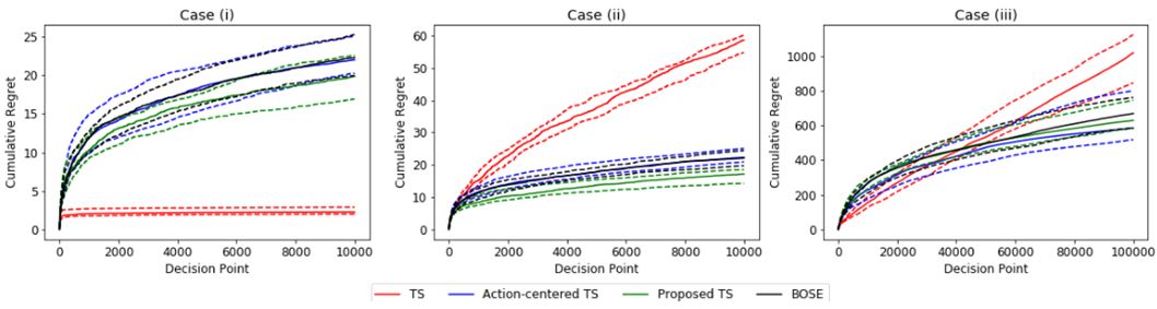
We conduct simulation studies to evaluate the proposed algorithm, the original TS algorithm Agrawal and Goyal, 2013, the action-centered TS (ACTS) algorithm (Greenewald et al., 2017) and the BOSE algorithm (Krishnamurthy et al., 2018). We set N=2N\!\!=\!\!2 or 66 and d=10d\!=\!10. We set the first action to be the base action, i.e., b1​(t)=0db_{1}(t)\!=\!0_{d} for all tt, and form the other context vectors as bi​(t)=[I⁡(i=2)​zi​(t)T,⋯,I⁡(i=N)​zi​(t)T]Tb_{i}(t)\!=\![I(i\!\!=\!\!2)z_{i}(t)^{T},\cdots,I(i\!\!=\!\!N)z_{i}(t)^{T}]^{T}, where zi​(t)∈ℝd′z_{i}(t)\in\mathbb{R}^{d^{\prime}}, d′=d/(N−1)d^{\prime}\!\!=\!\!d/(N\!-\!1), and zi​(t)z_{i}(t) is generated uniformly at random from the d′d^{\prime}-dimensional unit sphere. We generate ηi​(t)​∼i.i.d.​𝒩​(0,0.012)\eta_{i}(t)\overset{i.i.d.}{\sim}\mathcal{N}(0,0.01^{2}) and the rewards from (5), where we set μ=[−0.55,0.666,−0.09,−0.232,0.244,\mu=[-0.55,0.666,-0.09,-0.232,0.244, 0.55,−0.666,0.09,0.232,−0.244]T0.55,-0.666,0.09,0.232,-0.244]^{T} and consider three cases for ν⁡(t)\nu(t): (i) ν⁡(t)=0\nu(t)\!=\!0, (ii) ν⁡(t)=−ba∗​(t)​(t)T​μ,\nu(t)\!=\!-b_{a^{*}(t)}(t)^{T}\mu, (iii) ν⁡(t)=log⁡(t+1).\nu(t)\!=\!\mathrm{log}(t+1). We conduct 30 simulations in total for each case. Note that all four algorithms have one tuning parameter each that controls the degree of exploration. For the TS algorithms, the tuning parameter is vv in the variance of μ~​(t)\tilde{\mu}(t), and for the BOSE algorithm, ω\omega in the action elimination step. For each algorithm, we use the value of the parameter which incurs minimum median regret over 30 simulations. These values can be found by grid search.
Refer to caption
Figure 1: Median (solid), 1st and 3rd quartiles (dashed) of cumulative regret over 30 simulations when N=2N=2.
Refer to caption
Figure 2: Median (solid), 1st and 3rd quartiles (dashed) of cumulative regret over 30 simulations when N=6N=6.
Table 1: Median of R⁡(T)R(T) over 30 simulations.
Algorithms N=2N=2 N=6N=6
(i) (ii) (iii) (i) (ii) (iii)
TS 2 59 1020 7 70 9026
ACTS 22 22 586 200 246 3772
Proposed TS 20 17 629 55 29 1186
BOSE 22 22 669 —– —– —–

Figures 1 and 2 show the cumulative regret R⁡(t)R(t) according to time tt. The solid lines represent the median values and the dashed lines represent the lower and upper 25% percentiles. The values of R⁡(T)R(T) for each algorithm in each case are reported in Table 1. Figure 1 summarizes the results when N=2N=2. When ν⁡(t)=0\nu(t)=0, the original TS algorithm achieves lowest cumulative regret. The proposed method shows the second best performance in this case, while the BOSE and ACTS algorithms are also competitive. In cases where ν⁡(t)\nu(t) changes with time, the original TS algorithm hardly learns at all, while the three other methods developed under the nonparametric intercept term are competitive. When N=6N=6, Figure 2 exhibits a similar trend for the original TS and the proposed algorithms as in the N=2N=2 case. On the other hand, the BOSE algorithm has no explicit method so the results are not shown and the ACTS algorithm has much slower learning speed than the proposed TS method.

6 Real data analysis

We present the results of the proposed and existing methods using the R6A dataset provied by Yahoo! Webscope. The dataset is observational log data of user clicks from May 1st, 2009 to May 10th, 2009, which corresponds to 45,811,883 user visits. At every visit, one article was chosen uniformly at random from 20 articles (N=20N=20) and was displayed in the Featured tab of the Today module on Yahoo! front page. The reward ri​(t)r_{i}(t) is binary, taking value 11 if the visiting user clicked the ii-th article, and ri​(t)=0r_{i}(t)=0 otherwise. For each article ii, there is a context vector bi​(t)∈ℝ35b_{i}(t)\in\mathbb{R}^{35}, which is constituted of 5 extracted user features, 5 extracted article features and their products. The extracted features were constructed from high-dimensional raw data for user and article features using a dimension reduction method of Chu et al., 2009.

Evaluating a new reinforcement learning policy retrospectively using observational log data is a challenging task itself and calls for off-policy evaluation methods. This is because in the log data, the rewards of the actions that were not chosen by the original logging policy are missing. In our log data, only the rewards of articles chosen by the uniform random policy are observed.

Denote the policy that we want to evaluate as A and the total TT-trial reward of A as GA​(T):=𝔼⁡[∑t=1Tra⁡(t)​(t)]G_{\texttt{A}}(T):=\mathbb{E}\big[\sum_{t=1}^{T}r_{a(t)}(t)\big], where a⁡(t)a(t) is chosen by A. Li et al., 2011 proposed an offline evaluation algorithm for estimating GA​(T)G_{\texttt{A}}(T). Given the stream of events (𝒃={bi}i=1N,a,ra)(\boldsymbol{b}=\{b_{i}\}_{i=1}^{N},a,r_{a}) from log data, the algorithm picks up the events of which the chosen action aa matches the choice of A and stacks them into the history of A. Rewards in the history are used to construct the estimate G^A​(T)\hat{G}_{\texttt{A}}(T). In the case where A is an online learning policy, the history is used to update the action selection distribution of A as well. Under the condition that (𝒃⁡(t),r⁡(t))(\boldsymbol{b}(t),r(t)) are i.i.d. and the logging policy is the uniform random policy, G^A​(T)\hat{G}_{\texttt{A}}(T) is shown to be unbiased. We note that the i.i.d. condition does not cover the case where ν⁡(t)\nu(t) is adaptive to the past trials. Still, the conditional distribution of ν⁡(t)\nu(t) given 𝒃⁡(t)\boldsymbol{b}(t) is not restricted.

We evaluate the uniform random policy, TS algorithm and the proposed algorithm using the method of Li et al., 2011. We use data of May 1st, 2009 as tuning data to choose the optimal exploration parameter vv for the TS algorithm and the proposed algorithm, respectively. Then we conduct main analysis on data from May 2nd to May 10th, 2009. Note that the method of Li et al., 2011 picks up over 1/N=1/20{1}/{N}={1}/{20} of the log data. This corresponds to over T=1900000T=1900000. We fix the value of TT to T=1900000T=1900000 a priori, and conduct the evaluation algorithm for 10 times on the same data for each policy. Since the evaluated policies are all randomized algorithms, each of the 10 runs pick up different actions, giving 10 different estimates. We report the mean, 1st quartile and 3rd quartile of the estimates for each policy in Table 2.

Table 2: Mean, 1st quartile (1st Q.) and 3rd quartile (3rd Q.) of user clicks achieved by each policy over 10 runs.
Policies Mean 1st Q. 3rd Q.
Uniform policy 66696.7 66515.0 66832.8
TS algorithm 86907.0 85992.8 88551.3
Proposed TS 90689.7 90177.3 91166.3

We verify that the contextual bandit algorithms achieve substantially higher user click rates than the uniform random policy. Among the contextual bandit algorithms, the proposed algorithm increases the average user click rate by 4.4% compared to the original TS algorithm.

7 Concluding remarks

This paper proposes a new contextual MAB algorithm for a semiparametric reward model which is well suited to real problems where baseline rewards are bound to change with time. The proposed algorithm improves on existing methods that consider the same model. Simulation study and real data analysis demonstrate the advantage of the proposed method.

References

  • Abbasi-Yadkori et al., (2011) Abbasi-Yadkori, Y., Pál, D. and Szepesvári, C. Improved algorithms for linear stochastic bandits. In Advances in Neural Information Processing Systems, pp. 2312–2320, 2011.
  • Abramowitz and Stegun, (1964) Abramowitz, M. and Stegun, I.A. Handbook of mathematical functions with formulas, graphs, and mathematical tables. Washington, DC: National Bureau of Standards, 1964.
  • Agrawal and Goyal, (2013) Agrawal, S. and Goyal, N. Thompson sampling for contextual bandits with linear payoffs. In Proceedings of the 30th International Conference on Machine Learning, pp. 127–135, 2013.
  • Auer, (2002) Auer, P. Using confidence bounds for exploitation-exploration trade-offs. Journal of Machine Learning Research, 3:397–422, 2002.
  • Bercu and Touati, (2008) Bercu, B. and Touati, A. Exponential inequalities for self-normalized martingales with applications. The Annals of Applied Probability, 18(5):1848–1869, 2008.
  • Beygelzimer et al., (2011) Beygelzimer, A., Langford, J., Li, L., Reyzin, L., and Schapire, R.E. Contextual bandit algorithms with supervised learning guarantees. In Proceedings of the 14th International Conference on Artificial Intelligence and Statistics, pp. 19–26, 2011.
  • Chu et al., (2009) Chu, W., Park, S.T., Beaupre, T., Motgi, N., Phadke, A., Chakraborty, S. and Zachariah, J. A case study of behavior-driven conjoint analysis on Yahoo!: front page today module. In Proceedings of the 15th ACM SIGKDD international conference on Knowledge discovery and data mining, pp. 1097-1104, 2009.
  • Chu et al., (2011) Chu, W., Li, L., Reyzin, L. and Schapire, R.E. Contextual bandits with linear payoff functions. In Proceedings of the 14th International Conference on Artificial Intelligence and Statistics, pp. 208–214, 2011.
  • Dani et al., (2008) Dani, V., Hayes, T. P. and Kakade, S. M. Stochastic linear optimization under bandit feedback. In Conference on Learning Theory, pp. 355–-366, 2008.
  • de la Peña et al., (2004) de la Peña, V. H., Klass, M. J. and Lai, T. L. Self-normalized processes: exponential inequalities, moment bounds and iterated logarithm laws. Annals of Probability, 32(3A):1902–1933, 2004.
  • de la Peña et al., (2009) de la Peña ,V. H., Klass, M. J. and Lai, T. L. Theory and applications of multivariate self-normalized processes. Stochastic Processes and their Applications, 119(12):4210–4227, 2009.
  • Even-Dar et al., (2006) Even-Dar, E., Mannor, S. and Mansour, Y. Action elimination and stopping conditions for the multi-armed bandit and reinforcement learning problems. Journal of machine learning research, 7:1079-1105, 2006.
  • Ferreira et al., (2018) Ferreira, K., Simchi-Levi, D. and Wang, H. Online network revenue management using Thompson sampling. Operations Research, 66(6):1586–1602, 2018.
  • Greenewald et al., (2017) Greenewald, K., Tewari, A., Murphy, S. and Klasnja, P. Action centered contextual bandits. In Advances in Neural Information Processing Systems, pp. 5977–5985, 2017.
  • Kawale et al., (2015) Kawale, J., Bui, H.H., Kveton, B., Tran-Thanh, L. and Chawla, S. Efficient Thompson sampling for online matrix-factorization recommendation. In Advances in Neural Information Processing Systems, pp. 1297–1305, 2015.
  • Krishnamurthy et al., (2018) Krishnamurthy, A., Wu, Z. S. and Syrgkanis, V. Semiparametric contextual bandits. In Proceedings of the 35th International Conference on Machine Learning, 2018.
  • Lai and Robbins, (1985) Lai, T.L. and Robbins, H. Asymptotically efficient adaptive allocation rules. Advances in Applied Mathematics, 6(1):4–22, 1985.
  • Langford et al., (2008) Langford, J., Strehl, A. and Wortman, J. Exploration scavenging. In Proceedings of the 25th International Conference on Machine Learning, pp. 528–535, 2008.
  • Li et al., (2010) Li, L., Chu, W., Langford, J. and Schapire, R. E. A contextual-bandit approach to personalized news article recommendation. In Proceedings of the 19th International Conference on World wide web, pp. 661–670, 2010.
  • Li et al., (2011) Li, L., Chu, W., Langford, J. and Wang, X. Unbiased offline evaluation of contextual-bandit-based news article recommendation algorithms. In Proceedings of the 4th ACM International Conference on Web search and data mining, pp. 297–306, 2011.
  • Robbins, (1952) Robbins, H. Some aspects of the sequential design of experiments. Bulletin of the American Mathematical Society, 58(5):527–535, 1952.
  • Schwartz et al., (2017) Schwartz, E.M., Bradlow, E.T. and Fader, P.S. Customer acquisition via display advertising using multi-armed bandit experiments. Marketing Science, 36(4):500–522, 2017.
  • Tewari and Murphy, (2017) Tewari, A., and Murphy, S.A. From ads to interventions: contextual bandits in mobile health. In Mobile Health (pp. 495–517). Springer, Cham, 2017.
  • Thompson, (1933) Thompson, W.R. On the likelihood that one unknown probability exceeds another in view of the evidence of two samples. Biometrika, 25(3/4):285–294, 1933.
  • Yahoo, (2019) Yahoo! Webscope. Yahoo! Front Page Today Module User Click Log Dataset, version 1.0. http://webscope.sandbox.yahoo.com. Accessed: 09/01/2019.

Appendix

A Preliminaries

Lemma A.1.

(Abbasi-Yadkori et al., 2011, Lemma 11 of ) Let {Xt}t=1T\{X_{t}\}_{t=1}^{T} be a sequence in ℝd\mathbb{R}^{d} with ‖Xt‖2≤1||X_{t}||_{2}\leq 1, QQ a d×dd\times d positive definite matrix with d​e​t​(Q)≥1det(Q)\geq 1 and A⁡(t)=∑τ=1t−1Xτ​XτT.A(t)=\sum_{\tau=1}^{t-1}X_{\tau}X_{\tau}^{T}. Then, we have

∑t=1TXtT​{Q+A⁡(t)}−1​Xt≤2​log​(d​e​t​(Q+A⁡(T+1))d​e​t​(Q)).\sum_{t=1}^{T}X_{t}^{T}\{Q+A(t)\}^{-1}X_{t}\leq 2\mathrm{log}\Big(\frac{det(Q+A(T+1))}{det(Q)}\Big).
Lemma A.2.

(Bercu and Touati, 2008, Lemma 2.1 of) Let xx be a square integrable random variable with mean 00 and variance σ2>0.\sigma^{2}>0. Then,

𝔼⁡[exp⁡(x−12​x2−12​σ2)]≤1.\mathbb{E}\Big[\mathrm{exp}\Big(x-\frac{1}{2}x^{2}-\frac{1}{2}\sigma^{2}\Big)\Big]\leq 1.
Lemma A.3.

(de la Peña et al., 2009, Lemma 7 of ) Let Xτ∈ℝdX_{\tau}\in\mathbb{R}^{d} be ℱτ\mathcal{F}_{\tau}-measurable for some filtration {ℱτ}τ=1t,\{\mathcal{F}_{\tau}\}_{\tau=1}^{t}, 𝔼⁡[Xτ|ℱτ−1]=0,\mathbb{E}\big[X_{\tau}|\mathcal{F}_{\tau-1}\big]=0, and ‖Xτ‖2≤B||X_{\tau}||_{2}\leq B for some constant BB, τ=1,⋯,t.\tau=1,\cdots,t. Let cτ∈ℝc_{\tau}\in\mathbb{R} be ℱτ\mathcal{F}_{\tau}-measurable, |cτ|≤1|c_{\tau}|\leq 1 and Xτ⟂cτ|ℱτ−1.X_{\tau}\perp c_{\tau}|\mathcal{F}_{\tau-1}. Then for any λ∈ℝd\lambda\in\mathbb{R}^{d},

𝔼⁡[exp⁡{λT​∑τ=1tXτ​cτ−12​λT​(∑τ=1tXτ​XτT+∑τ=1t𝔼⁡[Xτ​XτT|ℱτ−1])​λ}]≤1.\mathbb{E}\Big[\mathrm{exp}\Big\{\lambda^{T}\sum_{\tau=1}^{t}X_{\tau}c_{\tau}-\frac{1}{2}\lambda^{T}\Big(\sum_{\tau=1}^{t}X_{\tau}X_{\tau}^{T}+\sum_{\tau=1}^{t}\mathbb{E}\big[X_{\tau}X_{\tau}^{T}|\mathcal{F}_{\tau-1}\big]\Big)\lambda\Big\}\Big]\leq 1.
Proof.

Taking x=λT​Xτ​cτx=\lambda^{T}X_{\tau}c_{\tau}, we have from Lemma A.2,

𝔼⁡[exp⁡{λT​Xτ​cτ−12​λT​(cτ2​Xτ​XτT+𝔼⁡[cτ2​Xτ​XτT|ℱτ−1])​λ}|ℱτ−1]≤1.\mathbb{E}\Big[\mathrm{exp}\Big\{\lambda^{T}X_{\tau}c_{\tau}-\frac{1}{2}\lambda^{T}\Big(c_{\tau}^{2}X_{\tau}X_{\tau}^{T}+\mathbb{E}\big[c_{\tau}^{2}X_{\tau}X_{\tau}^{T}|\mathcal{F}_{\tau-1}\big]\Big)\lambda\Big\}\Big|\mathcal{F}_{\tau-1}\Big]\leq 1.

Since cτ2≤1c_{\tau}^{2}\leq 1 and Xτ​XτTX_{\tau}X_{\tau}^{T} is positive semi-definite,

𝔼⁡[exp⁡{λT​Xτ​cτ−12​λT​(Xτ​XτT+𝔼⁡[Xτ​XτT|ℱτ−1])​λ}|ℱτ−1]≤1.\mathbb{E}\Big[\mathrm{exp}\Big\{\lambda^{T}X_{\tau}c_{\tau}-\frac{1}{2}\lambda^{T}\Big(X_{\tau}X_{\tau}^{T}+\mathbb{E}\big[X_{\tau}X_{\tau}^{T}|\mathcal{F}_{\tau-1}\big]\Big)\lambda\Big\}\Big|\mathcal{F}_{\tau-1}\Big]\leq 1.

∎

Lemma A.4.

(Abramowitz and Stegun, 1964) If Z∼𝒩⁡(m,σ2),Z\sim\mathcal{N}(m,\sigma^{2}), for any z≥1z\geq 1,

12​π​z​exp​(−z22)≤ℙ⁡(|Z−m|>z​σ)≤1π​z​exp​(−z22).\frac{1}{2\sqrt{\pi}z}\mathrm{exp}\Big(-\frac{z^{2}}{2}\Big)\leq\mathbb{P}\big(|Z-m|>z\sigma\big)\leq\frac{1}{\sqrt{\pi}z}\mathrm{exp}\Big(-\frac{z^{2}}{2}\Big).

B Proof of Theorem 4.2

The proof of Theorem 4.2 follows the proof sketch of Section 4.2.

B.1 Proof of (14)

Take cτ=(ν⁡(τ)+b¯​(τ)T​μ2).c_{\tau}=\Big(\frac{\nu(\tau)+\bar{b}(\tau)^{T}\mu}{2}\Big). Since 𝔼⁡[Xτ|ℱτ−1]=0,\mathbb{E}\big[X_{\tau}|\mathcal{F}_{\tau-1}\big]=0, |cτ|≤1,|c_{\tau}|\leq 1, and Xτ⟂cτ|ℱτ−1,X_{\tau}\perp c_{\tau}|\mathcal{F}_{\tau-1}, we can apply Lemma A.3, i.e., for any λ∈ℝd,\lambda\in\mathbb{R}^{d},

𝔼⁡[exp⁡{λT​∑τ=1t−1Xτ​cτ−12​λT​(∑τ=1t−1Xτ​XτT+∑τ=1t−1𝔼⁡[Xτ​XτT|ℱτ−1])​λ}]≤1.\mathbb{E}\Big[\mathrm{exp}\Big\{\lambda^{T}\sum_{\tau=1}^{t-1}X_{\tau}c_{\tau}-\frac{1}{2}\lambda^{T}\Big(\sum_{\tau=1}^{t-1}X_{\tau}X_{\tau}^{T}+\sum_{\tau=1}^{t-1}\mathbb{E}[X_{\tau}X_{\tau}^{T}|\mathcal{F}_{\tau-1}]\Big)\lambda\Big\}\Big]\leq 1.

B.2 Proof of Lemma 4.4

By Lemma A.3, for any λ∈ℝd\lambda\in\mathbb{R}^{d},

𝔼⁡[exp⁡{λT​∑τ=1t−112​Yτ−12​λT​(12​∑τ=1t−1Yτ​YτT+12​∑τ=1t−1𝔼⁡[Yτ​YτT|ℱτ−1])​λ}]≤1.\mathbb{E}\Big[\mathrm{exp}\Big\{\lambda^{T}\sum_{\tau=1}^{t-1}\frac{1}{\sqrt{2}}Y_{\tau}-\frac{1}{2}\lambda^{T}\Big(\frac{1}{2}\sum_{\tau=1}^{t-1}Y_{\tau}Y_{\tau}^{T}+\frac{1}{2}\sum_{\tau=1}^{t-1}\mathbb{E}\big[Y_{\tau}Y_{\tau}^{T}|\mathcal{F}_{\tau-1}\big]\Big)\lambda\Big\}\Big]\leq 1.

Here,

λT​Yτ​YτT​λ\displaystyle\lambda^{T}Y_{\tau}Y_{\tau}^{T}\lambda =λT​D​(τ)​μ​μT​D​(τ)​λ\displaystyle=\lambda^{T}D({\tau})\mu\mu^{T}D({\tau})\lambda
={(D⁡(τ)​λ)T​μ}2\displaystyle=\big\{\big(D(\tau)\lambda\big)^{T}\mu\big\}^{2}
≤μTμ(D(τ)λ)T(D(τ)λ)(∵Cauchy-Schwarz inequality)\displaystyle\leq\mu^{T}\mu\big(D(\tau)\lambda\big)^{T}\big(D(\tau)\lambda\big)~~(\because\text{Cauchy-Schwarz inequality})
≤(D⁡(τ)​λ)T​(D⁡(τ)​λ)=λT​D​(τ)2​λ,\displaystyle\leq\big(D(\tau)\lambda\big)^{T}\big(D(\tau)\lambda\big)=\lambda^{T}D(\tau)^{2}\lambda, (17)

and

λT​𝔼​[Yτ​YτT|ℱτ−1]​λ\displaystyle\lambda^{T}\mathbb{E}\big[Y_{\tau}Y_{\tau}^{T}|\mathcal{F}_{\tau-1}\big]\lambda ≤λT​𝔼​[D​(τ)2|ℱτ−1]​λ.\displaystyle\leq\lambda^{T}\mathbb{E}\big[D(\tau)^{2}|\mathcal{F}_{\tau-1}\big]\lambda. (18)

Let L=Xτ​XτTL=X_{\tau}X_{\tau}^{T} and K=𝔼⁡[Xτ​XτT|ℱτ−1].K=\mathbb{E}\big[X_{\tau}X_{\tau}^{T}|\mathcal{F}_{\tau-1}\big]. Then,

λT​D​(τ)2​λ\displaystyle\lambda^{T}D(\tau)^{2}\lambda =λT​(L−K)2​λ\displaystyle=\lambda^{T}\big(L-K\big)^{2}\lambda
=λT​L2​λ+λT​K2​λ+2​λT​L​(−K)​λ\displaystyle=\lambda^{T}L^{2}\lambda+\lambda^{T}K^{2}\lambda+2\lambda^{T}L(-K)\lambda
≤λTL2λ+λTK2λ+2λT​L2​λ​λT​K2​λ(∵Cauchy-Schwarz inequality)\displaystyle\leq\lambda^{T}L^{2}\lambda+\lambda^{T}K^{2}\lambda+2\sqrt{\lambda^{T}L^{2}\lambda~\lambda^{T}K^{2}\lambda}~~(\because\text{Cauchy-Schwarz inequality})
≤2​λT​L2​λ+2​λT​K2​λ.\displaystyle\leq 2\lambda^{T}L^{2}\lambda+2\lambda^{T}K^{2}\lambda. (19)

Also,

𝔼⁡[D​(τ)2|ℱτ−1]\displaystyle\mathbb{E}\big[D(\tau)^{2}|\mathcal{F}_{\tau-1}\big] =𝔼⁡[(L−K)2|ℱτ−1]\displaystyle=\mathbb{E}\big[(L-K)^{2}|\mathcal{F}_{\tau-1}\big]
=𝔼⁡[L2|ℱτ−1]−𝔼⁡[L|ℱτ−1]​K−K​𝔼​[L|ℱτ−1]+K2\displaystyle=\mathbb{E}\big[L^{2}|\mathcal{F}_{\tau-1}\big]-\mathbb{E}\big[L|\mathcal{F}_{\tau-1}\big]K-K\mathbb{E}\big[L|\mathcal{F}_{\tau-1}\big]+K^{2}
=𝔼[L2|ℱτ−1]−K2(∵𝔼[L|ℱτ−1]=K)\displaystyle=\mathbb{E}\big[L^{2}|\mathcal{F}_{\tau-1}\big]-K^{2}~~~(\because\mathbb{E}\big[L|\mathcal{F}_{\tau-1}\big]=K)
⇒λT​𝔼​[D​(τ)2|ℱτ−1]​λ\displaystyle\Rightarrow\lambda^{T}\mathbb{E}\big[D(\tau)^{2}|\mathcal{F}_{\tau-1}\big]\lambda ≤2​λT​𝔼​[D​(τ)2|ℱτ−1]​λ\displaystyle\leq 2\lambda^{T}\mathbb{E}\big[D(\tau)^{2}|\mathcal{F}_{\tau-1}\big]\lambda
=2​λT​𝔼​[L2|ℱτ−1]​λ−2​λT​K2​λ.\displaystyle=2\lambda^{T}\mathbb{E}\big[L^{2}|\mathcal{F}_{\tau-1}\big]\lambda-2\lambda^{T}K^{2}\lambda. (20)

Due to (17), (18), (19) and (20),

λT​(Yτ​YτT+𝔼⁡[Yτ​YτT|ℱτ−1])​λ\displaystyle\lambda^{T}\Big(Y_{\tau}Y_{\tau}^{T}+\mathbb{E}\big[Y_{\tau}Y_{\tau}^{T}|\mathcal{F}_{\tau-1}\big]\Big)\lambda ≤2​λT​(L2+𝔼⁡[L2|ℱτ−1])​λ\displaystyle\leq 2\lambda^{T}\Big(L^{2}+\mathbb{E}\big[L^{2}|\mathcal{F}_{\tau-1}\big]\Big)\lambda
≤2​λT​(Xτ​XτT+𝔼⁡[Xτ​XτT|ℱτ−1])​λ,\displaystyle\leq 2\lambda^{T}\Big(X_{\tau}X_{\tau}^{T}+\mathbb{E}\big[X_{\tau}X_{\tau}^{T}|\mathcal{F}_{\tau-1}\big]\Big)\lambda,

where the last inequality is due to L=Xτ​XτTL=X_{\tau}X_{\tau}^{T} and XτT​Xτ≤1X_{\tau}^{T}X_{\tau}\leq 1. Therefore, for any λ∈ℝd\lambda\in\mathbb{R}^{d},

𝔼⁡[exp⁡{λT​∑τ=1t−112​Yτ−12​λT​(∑τ=1t−1Xτ​XτT+∑τ=1t−1𝔼⁡[Xτ​XτT|ℱτ−1])​λ}]\mathbb{E}\Big[\mathrm{exp}\Big\{\lambda^{T}\sum_{\tau=1}^{t-1}\frac{1}{\sqrt{2}}Y_{\tau}-\frac{1}{2}\lambda^{T}\Big(\sum_{\tau=1}^{t-1}X_{\tau}X_{\tau}^{T}+\sum_{\tau=1}^{t-1}\mathbb{E}\big[X_{\tau}X_{\tau}^{T}|\mathcal{F}_{\tau-1}\big]\Big)\lambda\Big\}\Big]~~~~~~~~~~~~~~~~~~~~~~~~~~~~~~~~~~~~~~~~~~~~~
≤𝔼⁡[exp⁡{λT​∑τ=1t−112​Yτ−12​λT​(12​∑τ=1t−1Yτ​YτT+12​∑τ=1t−1𝔼⁡[Yτ​YτT|ℱτ−1])​λ}]\displaystyle\leq\mathbb{E}\Big[\mathrm{exp}\Big\{\lambda^{T}\sum_{\tau=1}^{t-1}\frac{1}{\sqrt{2}}Y_{\tau}-\frac{1}{2}\lambda^{T}\Big(\frac{1}{2}\sum_{\tau=1}^{t-1}Y_{\tau}Y_{\tau}^{T}+\frac{1}{2}\sum_{\tau=1}^{t-1}\mathbb{E}\big[Y_{\tau}Y_{\tau}^{T}|\mathcal{F}_{\tau-1}\big]\Big)\lambda\Big\}\Big]
≤1.\displaystyle\leq 1.

C Proof of Theorem 4.1

The proof of Theorem 4.1 follows the lines of Agrawal and Goyal, 2013 with some modifications. We present the whole proof.

  1. (a)

    The first stage is the derivation of a high-probability upper bound of |(bi​(t)−b¯​(t))T​(μ^​(t)−μ)||(b_{i}(t)-\bar{b}(t))^{T}(\hat{\mu}(t)-\mu)|. This is done in Theorem 4.2, which we restate here for concreteness.

    Theorem C.1.

    Let the event Eμ^​(t)E^{\hat{\mu}}(t) be defined as follows:

    Eμ^​(t)={∀i:|(bi​(t)−b¯​(t))T​(μ^​(t)−μ)|≤l⁡(t)​st,ic},E^{\hat{\mu}}(t)=\big\{\forall i:|\big(b_{i}(t)-\bar{b}(t)\big)^{T}(\hat{\mu}(t)-\mu)|\leq l(t)s_{t,i}^{c}\big\},

    where st,ic=(bi​(t)−b¯​(t))T​B​(t)−1​(bi​(t)−b¯​(t))s_{t,i}^{c}=\sqrt{\big(b_{i}(t)-\bar{b}(t)\big)^{T}B(t)^{-1}\big(b_{i}(t)-\bar{b}(t)\big)} and l⁡(t)=(2​R+6)​d​log​(6​t3/δ)+1l(t)=(2R+6)\sqrt{d\mathrm{log}(6t^{3}/\delta)}+1. Then for all t≥1t\geq 1, for any 0<δ<10<\delta<1, ℙ⁡(Eμ^​(t))≥1−δt2.\mathbb{P}(E^{\hat{\mu}}(t))\geq 1-\frac{\delta}{t^{2}}.

  2. (b)

    We next establish a high-probability upper bound for |(bi​(t)−b¯​(t))T​(μ~​(t)−μ^​(t))||(b_{i}(t)-\bar{b}(t))^{T}(\tilde{\mu}(t)-\hat{\mu}(t))| in the following Proposition C.2. The proof is a simple extension of Agrawal and Goyal, 2013, which uses Lemma A.4 for gaussian random variables.

    Proposition C.2.

    Let the event Eμ~​(t)E^{\tilde{\mu}}(t) be defined as follows:

    Eμ~​(t)={∀i:|(bi​(t)−b¯​(t))T​(μ~​(t)−μ^​(t))|≤m⁡(T)​st,ic},E^{\tilde{\mu}}(t)=\big\{\forall i:|\big(b_{i}(t)-\bar{b}(t)\big)^{T}(\tilde{\mu}(t)-\hat{\mu}(t))|\leq m(T)s_{t,i}^{c}\big\},

    where m⁡(T)=v​4​d​log​(T​d).m(T)=v\sqrt{4d\mathrm{log}(Td)}. Then for all t≥0t\geq 0, ℙ⁡(Eμ~​(t)|ℱt−1)≥1−1T2\mathbb{P}(E^{\tilde{\mu}}(t)|\mathcal{F}_{t-1})\geq 1-\frac{1}{T^{2}}.

    Proof.

    Note that given ℱt−1\mathcal{F}_{t-1}, the values of (bi​(t)−b¯​(t))\big(b_{i}(t)-\bar{b}(t)\big), B⁡(t)B(t) and μ^​(t)\hat{\mu}(t) are fixed. Then,

    |bic​(t)T​(μ~​(t)−μ^​(t))|\displaystyle|b_{i}^{c}(t)^{T}(\tilde{\mu}(t)-\hat{\mu}(t))| =|bic(t)TvB(t)−1/21vB(t)1/2(μ~(t)−μ^(t))|\displaystyle=|b_{i}^{c}(t)^{T}vB(t)^{-1/2}\frac{1}{v}B(t)^{1/2}(\tilde{\mu}(t)-\hat{\mu}(t))|
    ≤v​bic​(t)T​B​(t)−1​bic​(t)​‖1v​B​(t)1/2​(μ~​(t)−μ^​(t))‖2\displaystyle\leq v\sqrt{b_{i}^{c}(t)^{T}B(t)^{-1}b_{i}^{c}(t)}\Big|\Big|\frac{1}{v}B(t)^{1/2}(\tilde{\mu}(t)-\hat{\mu}(t))\Big|\Big|_{2}
    =v​st,ic​‖1v​B​(t)1/2​(μ~​(t)−μ^​(t))‖2\displaystyle=vs_{t,i}^{c}\Big|\Big|\frac{1}{v}B(t)^{1/2}(\tilde{\mu}(t)-\hat{\mu}(t))\Big|\Big|_{2}
    =v​st,ic​∑j=1d‖Zj​(t)‖22,\displaystyle=vs_{t,i}^{c}\sqrt{\sum_{j=1}^{d}||Z_{j}(t)||_{2}^{2}},

    where Zj​(t)|ℱt−1​∼i.i.d.​𝒩​(0,1)Z_{j}(t)|\mathcal{F}_{t-1}\overset{i.i.d.}{\sim}\mathcal{N}(0,1) and the first inequality is due to Cauchy-Schwarz inequality. Due to Lemma A.4, for fixed jj and z≥1z\geq 1,

    ℙ⁡(|Zj​(t)|>z|ℱt−1)≤1π​z​exp​(−z22)≤exp⁡(−z22).\mathbb{P}\big(|Z_{j}(t)|>z~|~\mathcal{F}_{t-1}\big)\leq\frac{1}{\sqrt{\pi}z}\mathrm{exp\Big(-\frac{z^{2}}{2}\Big)}\leq\mathrm{exp\Big(-\frac{z^{2}}{2}\Big)}.

    Setting exp(−z2/2)=1d​T2\mathrm{exp\big(-{z^{2}}/{2}\big)}=\frac{1}{dT^{2}}, we have z=2​log​(d​T2)≤2​log​(d2​T2)z=\sqrt{2\mathrm{log}(dT^{2})}\leq\sqrt{2\mathrm{log}(d^{2}T^{2})} =4​log​(d​T)=\sqrt{4\mathrm{log}(dT)}. Hence,

    ℙ⁡(|Zj​(t)|>4​l​o​g​(d​T)|ℱt−1)≤1d​T2\displaystyle\mathbb{P}\big(|Z_{j}(t)|>\sqrt{4\mathrm{log}(dT)}~|~\mathcal{F}_{t-1}\big)\leq\frac{1}{dT^{2}}
    ⇒ℙ(∀j:|Zj(t)|>4​l​o​g​(d​T)|ℱt−1)≤1T2.\displaystyle\Rightarrow\mathbb{P}\big(\forall j:|Z_{j}(t)|>\sqrt{4\mathrm{log}(dT)}~|~\mathcal{F}_{t-1}\big)\leq\frac{1}{T^{2}}.

    Thus, with probability at least 1−1T21-\frac{1}{T^{2}}, for all i=1,⋯,Ni=1,\cdots,N,

    |(bi​(t)−b¯​(t))T​(μ~​(t)−μ^​(t))|\displaystyle|\big(b_{i}(t)-\bar{b}(t)\big)^{T}(\tilde{\mu}(t)-\hat{\mu}(t))| ≤v​st,ic​4​d​log​(d​T)=m⁡(T)​st,ic.\displaystyle\leq vs_{t,i}^{c}\sqrt{4d\mathrm{log}(dT)}=m(T)s_{t,i}^{c}.

    ∎

  3. (c)

    Before proceeding, we divide the arms at each time into two groups: saturated and unsaturated arms. Let g⁡(T)=m⁡(T)+l⁡(T).g(T)=m(T)+l(T). An arm ii is saturated at time tt if

    (bi​(t)−b¯​(t))T​μ+g⁡(T)​st,ic<(ba∗​(t)​(t)−b¯​(t))T​μ,\big(b_{i}(t)-\bar{b}(t)\big)^{T}\mu+g(T)s_{t,i}^{c}<\big(b_{a^{*}(t)}(t)-\bar{b}(t)\big)^{T}\mu,

    and unsaturated otherwise. Note that the optimal arm a∗​(t)a^{*}(t) is unsaturated. Note also that from Stage (a) and Stage (b), (bi​(t)−b¯​(t))T​μ+g⁡(T)​st,ic(b_{i}(t)-\bar{b}(t))^{T}\mu+g(T)s_{t,i}^{c} is an upper bound of (bi​(t)−b¯​(t))T​μ~​(t)(b_{i}(t)-\bar{b}(t))^{T}\tilde{\mu}(t). Hence by definition, the saturated arms are the arms that have quite accurate values of (bi​(t)−b¯​(t))T​μ~​(t)(b_{i}(t)-\bar{b}(t))^{T}\tilde{\mu}(t) so that their upper bound is lower than (ba∗​(t)​(t)−b¯​(t))T​μ,(b_{a^{*}(t)}(t)-\bar{b}(t))^{T}\mu, enabling the algorithm to distinguish between them and the optimal arm.

  4. (d)

    Next, we show in Proposition C.3 that the probability of playing saturated arms is bounded by a function of the probability of playing unsaturated arms. The proof is a simple extension of Agrawal and Goyal, 2013.

    Proposition C.3.

    Let C⁡(t)C(t) be the set of saturated arms at time tt, i.e., C⁡(t)={i:(bi​(t)−b¯​(t))T​μ+g⁡(T)​st,ic<(ba∗​(t)​(t)−b¯​(t))T​μ}C(t)=\{i:\big(b_{i}(t)-\bar{b}(t)\big)^{T}\mu+g(T)s_{t,i}^{c}<\big(b_{a^{*}(t)}(t)-\bar{b}(t)\big)^{T}\mu\}. Given any filtration ℱt−1\mathcal{F}_{t-1} such that Eμ^​(t)E^{\hat{\mu}}(t) is true,

    ℙ⁡(a⁡(t)∈C⁡(t)|ℱt−1)≤1p​ℙ​(a⁡(t)∉C⁡(t)|ℱt−1)+1p​T2,\mathbb{P}\big(a(t)\in C(t)|\mathcal{F}_{t-1}\big)\leq\frac{1}{p}\mathbb{P}\big(a(t)\notin C(t)|\mathcal{F}_{t-1}\big)+\frac{1}{pT^{2}},

    where p=14​e​2​π.p=\frac{1}{4\mathrm{e}\sqrt{2}\sqrt{\pi}}.

    Proof.

    Since the algorithm pulls the arm argmax𝑖​{bi​(t)T​μ~​(t)},\underset{i}{\mathrm{argmax}}\{b_{i}(t)^{T}\tilde{\mu}(t)\}, if ba∗​(t)​(t)T​μ~​(t)>bj​(t)T​μ~​(t)b_{a^{*}(t)}(t)^{T}\tilde{\mu}(t)>b_{j}(t)^{T}\tilde{\mu}(t) for every j∈C⁡(t),j\in C(t), then a⁡(t)∉C⁡(t).a(t)\notin C(t). Hence,

    ℙ⁡(a⁡(t)∉C⁡(t)|ℱt−1)\displaystyle\mathbb{P}\big(a(t)\notin C(t)|\mathcal{F}_{t-1}\big) ≥ℙ(ba∗​(t)(t)Tμ~(t)>bj(t)Tμ~(t),∀j∈C(t)|ℱt−1)\displaystyle\geq\mathbb{P}\big(b_{a^{*}(t)}(t)^{T}\tilde{\mu}(t)>b_{j}(t)^{T}\tilde{\mu}(t),~\forall j\in C(t)|\mathcal{F}_{t-1}\big)
    =ℙ(ba∗​(t)c(t)Tμ~(t)>bjc(t)Tμ~(t),∀j∈C(t)|ℱt−1).\displaystyle=\mathbb{P}\big(b_{a^{*}(t)}^{c}(t)^{T}\tilde{\mu}(t)>b_{j}^{c}(t)^{T}\tilde{\mu}(t),~\forall j\in C(t)|\mathcal{F}_{t-1}\big). (21)

    If Eμ~​(t)E^{\tilde{\mu}}(t) is additionally true, for ∀j∈C⁡(t),\forall j\in C(t),

    bjc​(t)T​μ~​(t)\displaystyle b_{j}^{c}(t)^{T}\tilde{\mu}(t) ≤bjc(t)Tμ+g(T)st,jc(∵Eμ^(t)&Eμ~(t))\displaystyle\leq b_{j}^{c}(t)^{T}\mu+g(T)s_{t,j}^{c}~~~(\because E^{\hat{\mu}}(t)~\&~E^{\tilde{\mu}}(t))
    ≤ba∗​(t)c(t)Tμ.(∵definition of C(t))\displaystyle\leq b_{a^{*}(t)}^{c}(t)^{T}\mu.~~~(\because\text{definition of }C(t))

    Therefore,

    ℙ(ba∗​(t)c(t)Tμ~(t)>bjc(t)Tμ~(t),∀j∈C(t)|ℱt−1)+(1−ℙ(Eμ~(t)|ℱt−1))\displaystyle\mathbb{P}\big(b_{a^{*}(t)}^{c}(t)^{T}\tilde{\mu}(t)>b_{j}^{c}(t)^{T}\tilde{\mu}(t),~\forall j\in C(t)|\mathcal{F}_{t-1}\big)+\Big(1-\mathbb{P}\big(E^{\tilde{\mu}}(t)|\mathcal{F}_{t-1}\big)\Big)~~~~~~~~~~~~~~~~~
    ≥ℙ⁡(ba∗​(t)c​(t)T​μ~​(t)>ba∗​(t)c​(t)T​μ|ℱt−1).\displaystyle\geq\mathbb{P}\big(b_{a^{*}(t)}^{c}(t)^{T}\tilde{\mu}(t)>b_{a^{*}(t)}^{c}(t)^{T}\mu|\mathcal{F}_{t-1}\big). (22)

    Given Eμ^​(t),E^{\hat{\mu}}(t), |ba∗​(t)c​(t)T​(μ^​(t)−μ)|≤l⁡(T)​st,a∗​(t)c.|b_{a^{*}(t)}^{c}(t)^{T}(\hat{\mu}(t)-\mu)|\leq l(T)s_{t,a^{*}(t)}^{c}. Thus by Lemma A.4,

    (22)\displaystyle(\ref{eq2}) =ℙ⁡(ba∗​(t)c​(t)T​(μ~​(t)−μ^​(t))v​st,a∗​(t)c>ba∗​(t)c​(t)T​(μ−μ^​(t))v​st,a∗​(t)c|ℱt−1)\displaystyle=\mathbb{P}\Big(~\frac{b_{a^{*}(t)}^{c}(t)^{T}(\tilde{\mu}(t)-\hat{\mu}(t))}{vs_{t,a^{*}(t)}^{c}}>\frac{b_{a^{*}(t)}^{c}(t)^{T}(\mu-\hat{\mu}(t))}{vs_{t,a^{*}(t)}^{c}}\Big|\mathcal{F}_{t-1}\Big)
    ≥ℙ⁡(Z⁡(t)>l⁡(T)v|ℱt−1)\displaystyle\geq\mathbb{P}\Big(~Z(t)>\frac{l(T)}{v}\Big|\mathcal{F}_{t-1}\Big)
    ≥14​π​z​exp​(−z22)≥p,\displaystyle\geq\frac{1}{4\sqrt{\pi}z}\mathrm{exp}\Big(-\frac{z^{2}}{2}\Big)\geq{p}, (23)

    where Z⁡(t)|ℱt−1∼𝒩⁡(0,1)Z(t)|\mathcal{F}_{t-1}\sim\mathcal{N}(0,1) and z=l⁡(T)/v.z={l(T)}/v. Therefore, due to (21), (22), (23) and Proposition C.2,

    ℙ⁡(a⁡(t)∉C⁡(t)|ℱt−1)≥p−1T2.\mathbb{P}\big(a(t)\notin C(t)|\mathcal{F}_{t-1}\big)\geq p-\frac{1}{T^{2}}.
    ⇒ℙ⁡(a⁡(t)∈C⁡(t)|ℱt−1)ℙ⁡(a⁡(t)∉C⁡(t)|ℱt−1)+1T2≤1p.\Rightarrow\frac{\mathbb{P}\big(a(t)\in C(t)|\mathcal{F}_{t-1}\big)}{\mathbb{P}\big(a(t)\notin C(t)|\mathcal{F}_{t-1}\big)+\frac{1}{T^{2}}}\leq\frac{1}{p}.

    ∎

  5. (e)

    Next in Proposition C.4, we use Proposition C.3 and the definition of unsaturated arms to show that the regret can be bounded by a factor of st,a⁡(t)cs_{t,a(t)}^{c} in expectation.

    Proposition C.4.

    Given any filtration ℱt−1\mathcal{F}_{t-1} such that Eμ^​(t)E^{\hat{\mu}}(t) is true,

    𝔼⁡[r​e​g​r​e​t​(t)|ℱt−1]≤5​g​(T)p​𝔼​[st,a⁡(t)c|ℱt−1]+3​g​(T)p​T2.\mathbb{E}\big[regret(t)|\mathcal{F}_{t-1}\big]\leq\frac{5g(T)}{p}\mathbb{E}\big[s_{t,a(t)}^{c}|\mathcal{F}_{t-1}\big]+\frac{3g(T)}{pT^{2}}.
    Proof.

    Let a~​(t)=argmini∉C⁡(t)​st,ic\tilde{a}(t)=\underset{i\notin C(t)}{\mathrm{argmin}}~s_{t,i}^{c}. This value is determined by ℱt−1\mathcal{F}_{t-1}. Under both Eμ^​(t)E^{\hat{\mu}}(t) and Eμ~​(t)E^{\tilde{\mu}}(t),

    ba∗​(t)c​(t)T​μ\displaystyle b_{a^{*}(t)}^{c}(t)^{T}\mu =ba∗​(t)c​(t)T​μ−ba~​(t)c​(t)T​μ+ba~​(t)c​(t)T​μ\displaystyle=b_{a^{*}(t)}^{c}(t)^{T}\mu-b_{\tilde{a}(t)}^{c}(t)^{T}\mu+b_{\tilde{a}(t)}^{c}(t)^{T}\mu
    ≤g⁡(T)​st,a~​(t)c+ba~​(t)c​(t)T​μ\displaystyle\leq g(T)s_{t,\tilde{a}(t)}^{c}+b_{\tilde{a}(t)}^{c}(t)^{T}\mu
    ≤g⁡(T)​st,a~​(t)c+ba~​(t)c​(t)T​μ~​(t)+g⁡(T)​st,a~​(t)c\displaystyle\leq g(T)s_{t,\tilde{a}(t)}^{c}+b_{\tilde{a}(t)}^{c}(t)^{T}\tilde{\mu}(t)+g(T)s_{t,\tilde{a}(t)}^{c}
    ≤2​g​(T)​st,a~​(t)c+ba⁡(t)c​(t)T​μ~​(t)\displaystyle\leq 2g(T)s_{t,\tilde{a}(t)}^{c}+b_{a(t)}^{c}(t)^{T}\tilde{\mu}(t)
    ≤2​g​(T)​st,a~​(t)c+ba⁡(t)c​(t)T​μ+g⁡(T)​st,a⁡(t)c\displaystyle\leq 2g(T)s_{t,\tilde{a}(t)}^{c}+b_{a(t)}^{c}(t)^{T}{\mu}+g(T)s_{t,a(t)}^{c}
    ⇒r​e​g​r​e​t​(t)\displaystyle\Rightarrow regret(t) ≤2​g​(T)​st,a~​(t)c+g⁡(T)​st,a⁡(t)c,\displaystyle\leq 2g(T)s_{t,\tilde{a}(t)}^{c}+g(T)s_{t,a(t)}^{c},

    where the first inequality follows from the definition of unsaturated arms, the second and fourth inequalities from Eμ^​(t)E^{\hat{\mu}}(t) and Eμ~​(t)E^{\tilde{\mu}}(t), and the third inequality from the action selection mechanism. Therefore, given ℱt−1\mathcal{F}_{t-1} such that Eμ^​(t)E^{\hat{\mu}}(t) holds,

    𝔼⁡[r​e​g​r​e​t​(t)|ℱt−1]\displaystyle\mathbb{E}\big[regret(t)|\mathcal{F}_{t-1}\big] ≤2​g​(T)​st,a~​(t)c+g⁡(T)​𝔼​[st,a⁡(t)c|ℱt−1]+1−ℙ⁡(Eμ~​(t)|ℱt−1)\displaystyle\leq 2g(T)s_{t,\tilde{a}(t)}^{c}+g(T)\mathbb{E}\big[s_{t,a(t)}^{c}|\mathcal{F}_{t-1}\big]+1-\mathbb{P}(E^{\tilde{\mu}}(t)|\mathcal{F}_{t-1})
    ≤2​g​(T)​st,a~​(t)c+g⁡(T)​𝔼​[st,a⁡(t)c|ℱt−1]+1T2.\displaystyle\leq 2g(T)s_{t,\tilde{a}(t)}^{c}+g(T)\mathbb{E}\big[s_{t,a(t)}^{c}|\mathcal{F}_{t-1}\big]+\frac{1}{T^{2}}. (24)

    Here,

    st,a~​(t)c\displaystyle s_{t,\tilde{a}(t)}^{c} =st,a~​(t)c​{ℙ⁡(a⁡(t)∈C⁡(t)|ℱt−1)+ℙ⁡(a⁡(t)∉C⁡(t)|ℱt−1)}\displaystyle=s_{t,\tilde{a}(t)}^{c}\big\{\mathbb{P}(a(t)\in C(t)|\mathcal{F}_{t-1})+\mathbb{P}(a(t)\notin C(t)|\mathcal{F}_{t-1})\big\}
    ≤st,a~​(t)c​{2p​ℙ​(a⁡(t)∉C⁡(t)|ℱt−1)+1p​T2}\displaystyle\leq s_{t,\tilde{a}(t)}^{c}\Big\{\frac{2}{p}\mathbb{P}(a(t)\notin C(t)|\mathcal{F}_{t-1})+\frac{1}{pT^{2}}\Big\}
    =2p𝔼(st,a~​(t)cI{a(t)∉C(t)}|ℱt−1)+st,a~​(t)cp​T2\displaystyle=\frac{2}{p}\mathbb{E}\big(s_{t,\tilde{a}(t)}^{c}I\{a(t)\notin C(t)\}\big|\mathcal{F}_{t-1}\big)+\frac{s_{t,\tilde{a}(t)}^{c}}{pT^{2}}
    ≤2p𝔼(st,a⁡(t)cI{a(t)∉C(t)}|ℱt−1)+st,a~​(t)cp​T2\displaystyle\leq\frac{2}{p}\mathbb{E}\big(s_{t,{a}(t)}^{c}I\{a(t)\notin C(t)\}\big|\mathcal{F}_{t-1}\big)+\frac{s_{t,\tilde{a}(t)}^{c}}{pT^{2}}
    ≤2p​𝔼​(st,a⁡(t)c|ℱt−1)+1p​T2,\displaystyle\leq\frac{2}{p}\mathbb{E}\big(s_{t,{a}(t)}^{c}\big|\mathcal{F}_{t-1}\big)+\frac{1}{pT^{2}},

    where the first inequality is due to Proposition C.3 and the second inequality is due to the definition of a~​(t)\tilde{a}(t). Combining this result with (24), we have

    𝔼⁡[r​e​g​r​e​t​(t)|ℱt−1]\displaystyle\mathbb{E}\big[regret(t)|\mathcal{F}_{t-1}\big] ≤5​g​(T)p​𝔼​(st,a⁡(t)c|ℱt−1)+3​g​(T)p​T2.\displaystyle\leq\frac{5g(T)}{p}\mathbb{E}\big(s_{t,{a}(t)}^{c}\big|\mathcal{F}_{t-1}\big)+\frac{3g(T)}{pT^{2}}.

    ∎

  6. (f)

    Let Mt=r​e​g​r​e​t​(t)​I​(Eμ^​(t))−5​g​(T)p​st,a⁡(t)c−3​g​(T)p​T2.M_{t}=regret(t)I(E^{\hat{\mu}}(t))-\frac{5g(T)}{p}s_{t,a(t)}^{c}-\frac{3g(T)}{pT^{2}}. Then |Mt||M_{t}| is bounded by 9​g​(T)p.\frac{9g(T)}{p}. Also, due to Proposition C.4, {Mt}t=1T\{M_{t}\}_{t=1}^{T} is a bounded super-martingale difference process with respect to the filtration {ℱt}t=1T\{\mathcal{F}_{t}\}_{t=1}^{T}. Hence by Azuma-Hoeffding’s inequality, for any a≥0,a\geq 0,

    ℙ⁡(∑t=1TMt≥a)≤exp⁡(−a22​∑t=1Tct2),\mathbb{P}\big(\sum_{t=1}^{T}M_{t}\geq a\big)\leq\mathrm{exp}\Big(-\frac{a^{2}}{2\sum_{t=1}^{T}c_{t}^{2}}\Big),

    where ct=9p​g​(T).c_{t}=\frac{9}{p}g(T). Setting exp⁡(−a22​∑t=1Tct2)=δ2\mathrm{exp}\Big(-\frac{a^{2}}{2\sum_{t=1}^{T}c_{t}^{2}}\Big)=\frac{\delta}{2}, we have a=9p​g​(T)​2​T​log​(2δ).a=\frac{9}{p}g(T)\sqrt{2T\mathrm{log}\big(\frac{2}{\delta}\big)}. Thus with probability at least 1−δ2,1-\frac{\delta}{2},

    ∑t=1Tr​e​g​r​e​t​(t)​I​(Eμ^​(t))\displaystyle\sum_{t=1}^{T}regret(t)I(E^{\hat{\mu}}(t)) ≤5​g​(T)p​∑t=1Tst,a⁡(t)c+3​g​(T)p​T+9p​g​(T)​2​T​l​o​g​(2δ).\displaystyle\leq\frac{5g(T)}{p}\sum_{t=1}^{T}s_{t,a(t)}^{c}+\frac{3g(T)}{pT}+\frac{9}{p}g(T)\sqrt{2Tlog\big(\frac{2}{\delta}\big)}. (25)

    In Proposition C.5, we show that ∑t=1Tst,a⁡(t)c≤2​d​T​log​(1+T/d)\sum_{t=1}^{T}s_{t,a(t)}^{c}\leq\sqrt{2dT\mathrm{log}(1+T/d)} using Lemma A.1.

    Proposition C.5.

    ∑t=1Tst,a⁡(t)c≤2​d​T​log​(1+T/d).\sum_{t=1}^{T}s_{t,a(t)}^{c}\leq\sqrt{2dT\mathrm{log}(1+T/d)}.

    Proof.

    Take Xt=ba⁡(t)​(t)−b¯​(t)X_{t}=b_{a(t)}(t)-\bar{b}(t), Q=IdQ=I_{d}, and A⁡(t)=∑τ=1t−1Xτ​XτTA(t)=\sum_{\tau=1}^{t-1}X_{\tau}X_{\tau}^{T}. Then by Jensen’s inequality and Lemma A.1,

    ∑t=1Tst,a⁡(t)c\displaystyle\sum_{t=1}^{T}s_{t,a(t)}^{c} ≤T​∑t=1T{st,a⁡(t)c}2(∵ Jensen’s inequality)\displaystyle\leq\sqrt{T\sum_{t=1}^{T}\{s_{t,a(t)}^{c}\}^{2}}~~(\because\text{ Jensen's inequality})
    =T​∑t=1TXtT​B​(t)−1​Xt\displaystyle=\sqrt{T\sum_{t=1}^{T}X_{t}^{T}B(t)^{-1}X_{t}}
    ≤T​∑t=1TXtT​{Q+A⁡(t)}−1​Xt(∵B(t)≻Q+A(t))\displaystyle\leq\sqrt{T\sum_{t=1}^{T}X_{t}^{T}\{Q+A(t)\}^{-1}X_{t}}~~(\because B(t)\succ Q+A(t))
    ≤2​T​log⁡(d​e​t​(Q+A⁡(T+1))d​e​t​(Q))(∵ Lemma A.1)\displaystyle\leq\sqrt{2T\mathrm{\log}\Big(\frac{det(Q+A(T+1))}{det(Q)}\Big)}~~(\because\text{ Lemma \ref{boundons}})
    ≤2​d​T​log⁡(1+Td).(∵ determinant-trace inequality.)\displaystyle\leq\sqrt{2dT\mathrm{\log}\Big(1+\frac{T}{d}\Big)}.~~(\because\text{ determinant-trace inequality.})

    ∎

    Due to (25), Proposition C.5 and the definitions of pp and g⁡(T)g(T), we have with probability at least 1−δ21-\frac{\delta}{2},

    ∑t=1Tr​e​g​r​e​t​(t)​I​(Eμ^​(t))≤O⁡(d3/2​T​log⁡(T​d)​log​(T/δ)​(log⁡(1+T/d)+log⁡(1/δ))).\sum_{t=1}^{T}regret(t)I(E^{\hat{\mu}}(t))\leq O\Big(d^{3/2}\sqrt{T}\sqrt{\mathrm{log}(Td)\mathrm{log}(T/\delta)}\big(\sqrt{\mathrm{log}(1+T/d)}+\sqrt{\mathrm{log}(1/\delta)}\big)\Big).

    Since Eμ^​(t)E^{\hat{\mu}}(t) holds for all tt with probability at least 1−δ21-\frac{\delta}{2} (Theorem C.1), r​e​g​r​e​t​(t)​I​(Eμ^​(t))=r​e​g​r​e​t​(t)regret(t)I(E^{\hat{\mu}}(t))=regret(t) for all tt with probability at least 1−δ21-\frac{\delta}{2}. Hence, with probability at least 1−δ1-\delta,

    R⁡(T)≤O⁡(d3/2​T​log⁡(T​d)​log​(T/δ)​(log⁡(1+T/d)+log⁡(1/δ))).R(T)\leq O\Big(d^{3/2}\sqrt{T}\sqrt{\mathrm{log}(Td)\mathrm{log}(T/\delta)}\big(\sqrt{\mathrm{log}(1+T/d)}+\sqrt{\mathrm{log}(1/\delta)}\big)\Big).