Hybrid Einstein-Langevin Approach for Microscopic formulation of Viscous Drag: An Alternative to the Langevin EquationPreprint: UATP/1806

The behavior of a microscopically-visible Brownian particle (about a micron in diameter such as human red blood cell), first successfully formulated by Einstein Einstein-BrownianMotion, is perhaps the easiest prototypical behavior that appears in many nonequilibrium (NEQ) systems, where we encounter nonuniformity due to length scales of its constituents. Einstein assumed that a Brownian particle (BP) can be simply described by its stochastic center of mass position $\mathbf{r}$ for its specification and by ignoring the center of mass momentum and the specification of its constituent atoms or molecules. The diffusion of the BP obeys a diffusion equation, i.e., a Fokker–Planck equation describing stochasticity in the ensemble picture Keizer, which Einstein solved in equilibrium (EQ). Langevin Langevin later provided a very different formulation of the same motion as a stochastic process by applying Newton’s second law $Md^{2}\mathbf{r}/dt^{2}=\mathbf{F}(t)$ to the BP of mass $M$, by dividing $\mathbf{F}$ into a systematic viscous force $\mathbf{F}_{\text{f}}(t)$ and a stochastic force $\boldsymbol{\xi}(t)$ to each particular realization of the Brownian motion; see Chandrasekhar Chandrasekhar for an elegant discussion and inherent assumptions.

The distinct approaches by Einstein and Langevin have developed into mathematically distinct but physically equivalent ways (Fokker-Planck versus Langevin) to investigate stochastic processes Keizer. The approach by Einstein adopts a probabilistic approach to capture thermodynamic stochasticity and results in ensemble averages such as the root-mean-square displacement but dynamics is not a central issue. In contrast, Langevin’s approach starts with the dynamical equation in which $\mathbf{F}_{\text{f}}(t)$ is a thermodynamic average systematic force associated with dissipation (thus, satisfying the second law), while stochasticity is controlled by $\boldsymbol{\xi}(t)$ having a probability distribution of a $\delta$-correlated white Gaussian noise determined by its first two moments Chandrasekhar; they are its zero mean and constant standard deviation. This means that the Langevin force $\boldsymbol{\xi}(t)$ defines a stationary process because the probability distribution does not change in time, a well-known property of white noise. In the absence of the stochastic force, the velocity vanishes as $t\rightarrow\infty$ due to the viscous force. Langevin used this observation to justify the inclusion of the stochastic force Langevin. Such a separation is one of the basic assumptions as discussed by Chandrasekhar Chandrasekhar, Mazur, and Pomeau and Piasecki Pomeau.

It is not surprising that the Langevin equation now plays a dominant role in the development of the modern microscopic nonequilibrium (NEQ) stochastic thermodynamics Sekimoto; Sekimoto-Book; Seifert; Seifert-Rev, where attempt has been to extend the (macroscopic) first law of thermodynamics to the level of microstates. (All quantities at the microstate level are called microquantities as opposed to their ensemble averages, which we call macroquantities.) This requires introducing the concept of microwork and microheat for a microstate Gujrati-GeneralizedWork; Gujrati-GeneralizedWork-Expanded; their ensemble averages will be called macrowork or simply work and macroheat or simply heat in the macroscopic NEQ thermodynamics (NEQT) deGroot; Prigogine; Coleman. The concept of microwork and microheat seems to play a central role at diverse length scales from mesoscopic to macroscopic lengths Bochkov; Jarzynski; Crooks; Pitaevskii; Sekimoto; Sekimoto-Book; Seifert; Lebowitz; Alicki; see also some recent reviews Seifert-Rev; Maruyama.

The Langevin equation in one dimension is given by

with $\gamma>0$ in the systematic force to give rise to dissipation according to the second law, and $\xi(t)$ is the Gaussian white force independent of the state of the system Mazur. Both $\gamma$ and $\xi(t)$ are independent of the position and velocity of the BP so the two forces are independent despite arising from the interaction of the BP with its surroundings. Chandrasekhar Chandrasekhar emphasizes $\xi(t)$ as a characteristic of a BP, which undergoes rapid fluctuations over an interval $\Delta t$ over which $v$ only undergoes a small variation. Assuming Stokes’ law for a spherical Brownian particle of radius $a$, we have $\gamma=6\pi a\eta>0$, where $\eta$ is the viscosity of the surrounding fluid. It follows that we can identify a ”linear dimension” $l$ of a BP so that we can write $\gamma=\eta l$. In the stochastic energetics proposed by Sekimoto Sekimoto; Sekimoto-Book, this equation is taken to apply to each realization (microstate) of the Brownian motion, with $\gamma$ still satisfying $\gamma>0$.

In the absence of $\xi(t)$, and with $v_{0}$ as the initial velocity $v(0)$, we have

whereas in equilibrium ($t\rightarrow\infty$) we expect $\left\langle v^{2}\right\rangle=T/M$ from the equipartition theorem from the ensemble average over all possible values of $v$ or for that matter $v_{0}$. Therefore Langevin assumed the existence of $\xi(t)$, whereupon one needs to perform two distinct and independent averages over $v_{0}$ and $\xi$ at each time. The equipartition theorem is always fulfilled in Einstein’s approach Einstein-BrownianMotion being based on equilibrium thermodynamics.

We now propose an alternative approach to study each realization $\mathfrak{m}_{k}$ of the Brownian particle, which is a hybrid of the above two approaches in that we do not need $\xi(t)$ but the thermodynamic stochasticity appears due to the ensemble average as done by Einstein, and follows the standard formulation for a statistical system (Landau, for example) by considering the ensemble average of a quantity such as the velocity $\left\{\mathbf{v}_{k}\right\}$ over various microstates $\left\{\mathfrak{m}_{k}\right\}$ at each instant. Thus, $\mathbf{v}$ becomes a random variable whose outcomes are $\{\mathbf{v}_{k}\}$ on $\{\mathfrak{m}_{k}\}$. As microstate probabilities $p_{k}$ continue to change, the ensemble average is not stationary as for the white Langevin force.

The microforce $F_{k}$, see Eq. (6), associated with $\mathfrak{m}_{k}$ is the outcome of some random microforce and the macroforce, the ensemble average, is the systematic force of a particular sign in the Langevin equation. The non-vanishing fluctuations, see Eqs. (8a,8b), in $F_{k}$ even in equilibrium demonstrates that these outcomes have both signs. However, instead of considering $F_{k}$, we consider the microwork $d_{\text{i}}W_{k}$ done by it, whose average $d_{\text{i}}W\geq 0$ ($\gamma>0$) in accordance with the second law. The microwork $d_{\text{i}}W_{k}$, being specific to $\mathfrak{m}_{k}$, has a unique value that is independent of $p_{k}$ but changes over microstates.

Here we take a major departure from Langevin’s approach by not restricting the sign of $d_{\text{i}}W_{k}$ over all microstates for the simple reason that the second law is not applicable at the level of microstates; the law only emerges as the ensemble average is taken as is well known; see also Gujrati-GeneralizedWork; Gujrati-GeneralizedWork-Expanded for a clear demonstration. In the context of the Langevin equation, this means that $\gamma$ will be of either sign so that for some microstate, $v(t)$ in Eq. (2) may decrease and go to zero, while for others, it may increase in magnitude and diverge to infinity, as $t\rightarrow\infty$, with the condition that $\left\langle v^{2}\right\rangle$ will satisfy the equipartition theorem as we will demonstrate. We use the version NEQT that we have developed recently Gujrati-GeneralizedWork; Gujrati-GeneralizedWork-Expanded and briefly discussed below. We also derive the equations of motion using Newton’s second law; see Eqs. (7a,7b).

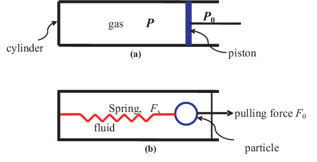
We consider the two examples (a) and (b) in Fig. 1 as our system $\Sigma$ and treat the piston or the particle as a Brownian particle (BP) of mass $M$. We assume that the piston in (a) may be either mesoscopic or microscopic, while the particle in (b) will be assumed to denote a mesoscopic particle of micron-like size. We will establish in our approach that both experience fluctuating Brownian motion, except that for the macroscopic size piston, it is not noticeable because of its macroscopic mass. We follow Einstein and focus on the center-of-mass (CM) of the BP, and denote rest of $\Sigma$ by excluding the BP by $\Sigma_{\text{R}}$. Let $V$ denote the volume of $\Sigma$ and $\mathbf{P}_{\text{BP}}$ and $\mathbf{P}_{\text{R}}$ the linear momenta of the BP and $\Sigma_{\text{R}}$, respectively. We assume that $\Sigma$ is stationary in the lab-frame so that

the medium $\widetilde{\Sigma}$ is also stationary. We will treat the piston problem for simplicity as it is commonly discussed in introductory physics. Let $\mathbf{x}$ denote a phase point in the phase space of $\Sigma$ so that the Hamiltonian of the system is written as $\mathcal{H}(\left.\mathbf{x}\right|V,\mathbf{P}_{\text{BP}},\mathbf{P}_{\text{R}})$ in which $V,\mathbf{P}_{\text{BP}}$ and $\mathbf{P}_{\text{R}}$ appear as parameters: the variations $dV,d\mathbf{P}_{\text{BP}}$ and $d\mathbf{P}_{\text{R}}$ change the value of $\mathcal{H}$; this change represents the generalized work $dW$ done by the system as shown elsewhere Gujrati-Heat-Work0; Gujrati-Heat-Work; Gujrati-I; Gujrati-II; Gujrati-III; Gujrati-Entropy1; Gujrati-Entropy2. Introducing the system-intrinsic (SI) ”mechanical forces” obtained directly from the SI-Hamiltonian

The generalized macrowork is now $dW=PdV-\mathbf{F}_{\text{BP}}\mathbf{\cdot}d\mathbf{R}$ and the generalized macroheat is $dQ=TdS$. We can now write $dE=dQ-dW$, which expresses the first law in terms of the generalized quantities. This expresses an important fact: the two terms in it denote independent variations of the energy $E$: $dQ$ denotes the change due to entropy variation and $dW$ isentropic variation (constant entropy). This allows us to deal with $dW$ as a purely mechanical ($dS=0$) quantity resulting in microstate energies, and $dQ$ as due to variations in microstate probabilities Gujrati-GeneralizedWork; Gujrati-GeneralizedWork-Expanded. which we summarize below for the benefit of the reader. For convenience, we treat $\mathbf{x}$ as discrete and use $k$ for it in the following. The average energy $E$ is defined in terms of microstate energies $E_{k}=E_{k}(V,\mathbf{P}_{\text{BP}})$ [or equivalently $E_{k}=E_{k}(V,\mathbf{R})$] and microstate probabilities $p_{k}$ as an ensemble average $\left\langle E\right\rangle$, written simply as $E\doteq{\textstyle\sum\nolimits_{k}}E_{k}p_{k},$ so that $dE={\textstyle\sum\nolimits_{k}}E_{k}dp_{k}+{\textstyle\sum\nolimits_{k}}p_{k}dE$, where $dE_{k}=(\partial E_{k}/\partial V)dV+(\partial E_{k}/\partial\mathbf{P}_{\text{BP}})\mathbf{\cdot}d\mathbf{P}_{\text{BP}}$; compare with Eqs. (4a) and (4b) after replacing $\mathbf{x}$ with $k$. (Recall that we can also use $\mathbf{R}$ instead of $\mathbf{P}_{\text{BP}}$ as an argument in $E_{k}$.) The first sum in $dE$ involves $dp_{k}$ at fixed $E_{k}$, and evidently corresponds to the entropy change $dS$. This sum denotes the generalized heat $dQ$. The second sum involves $dE_{k}$ at fixed $p_{k}$, and evidently corresponds to $dS=0$. As $dE_{k}$ is due to parameter changes in the Hamiltonian, it is related to the generalized work $(-dW_{k})$, which is the analog of Eq. (4d) for microstates. Its average gives rise to $(-dW)$, which then justifies the above rendition of the first law.

The exchange work is $d_{\text{e}}W=P_{0}dV$ and the irreversible work is $d_{\text{i}}W\doteq dW-d_{\text{e}}W$ associated with $\Sigma$ is

The inequality is in accordance with the second law Gujrati-GeneralizedWork; Gujrati-GeneralizedWork-Expanded. Similarly, the exchange heat with $\widetilde{\Sigma}$ is $d_{\text{e}}Q=T_{0}d_{\text{e}}S$ and the irreversible heat is $d_{\text{i}}Q\doteq dQ-d_{\text{e}}Q=(T-T_{0})d_{\text{e}}S+Td_{\text{i}}S~\mathbf{\geq}0$. Again, the last inequality is in accordance with the second law Gujrati-GeneralizedWork; Gujrati-GeneralizedWork-Expanded. As the first law can also be written as $dE=d_{\text{e}}Q-d_{\text{e}}W$, we must have $d_{\text{i}}Q=d_{\text{i}}W$ in magnitude, even though one is caused by changes in the probabilities and the other one by changes in microstate energies.

The irreversible contributions in $d_{\text{i}}W$ are due to some kind of ”force” imbalance as pointed out recently Gujrati-GeneralizedWork; Gujrati-GeneralizedWork-Expanded. Away from equilibrium, $P\neq P_{0}$ so the pressure imbalance $\Delta P\doteq P-P_{0}$ within $\Sigma$ determines the the first irreversible contribution in $d_{\text{i}}W$ above. Similarly, the average force and the relative velocity vanish in equilibrium ($\mathbf{F}_{\text{BP}}=0,\mathbf{V}=0$) so away from equilibrium, $\mathbf{F}_{\text{BP}}$ or $\mathbf{V}$ represents the force imbalance or the relative velocity imbalance and determines the second irreversible contribution $-\mathbf{F}_{\text{BP}}\mathbf{\cdot}d\mathbf{R}$ or $-\mathbf{V\cdot}d\mathbf{P}_{\text{BP}}$ in $d_{\text{i}}W$. From now on, we will assume $F_{0}$ and $F_{\text{s}}$ to be identically zero for simplicity for the particle as we wish to pursue the consequences of the relative velocity.

It follows from the second law that each term on the right side in Eq. (5) must be nonnegative so that $d_{\text{i}}W_{\text{f,BP}}\equiv-\mathbf{V\cdot}d\mathbf{P}_{\text{BP}}=-\mathbf{F}_{\text{BP}}\mathbf{\cdot}d\mathbf{R}\geq 0$; here, f is for friction. Hence, we can express $\mathbf{F}_{\text{BP}}=-\mathbf{V}f(V^{2},t)$, where $f(V^{2},t)>0$ is an even function of $\mathbf{V}$ at each instant so that $d_{\text{i}}W_{\text{f,BP}}=f(V^{2},t)\mathbf{V\cdot}d\mathbf{R}\geq 0$. To make connection with the Langevin equation, we will assume $f$ to be a power series with $f(0,t)=\gamma(t)$, which Langevin takes to be a constant so that $d_{\text{i}}W_{\text{f,BP}}\simeq\gamma\mathbf{V\cdot}d\mathbf{R}$ is the frictional work in a small-velocity approximation. The above discussion provides a thermodynamic justification of the viscous drag in the Langevin equation.

It follows from Eqs. (4a) and (4c) that the microanalog of $P$ is $P_{k}$, which differs from $P$ and the fluctuations $\Delta P\doteq P_{k}-P$ determine the mean square fluctuation $\left\langle(\Delta P)^{2}\right\rangle>0$ Gujrati-GeneralizedWork; Gujrati-GeneralizedWork-Expanded. It is known from equilibrium statistical mechanics that this fluctuation $\left\langle(\Delta P)^{2}\right\rangle_{\text{eq}}=-T(\partial P/\partial V)_{S}$ in EQ for $P=P_{0}$ is not identically zero Landau so $P_{k}\neq P$ in general. Similarly, there are fluctuations in $\mathbf{F}_{k\text{,BP}}$ or $\mathbf{V}_{k\text{,BP}}$ (the analog of $P_{k}$) around the average $\mathbf{F}_{\text{BP}}$ or $\mathbf{V}_{\text{BP}}$, which are always present; see Eqs. (8a-8b). In equilibrium, the average force and the average relative velocity vanish: $\mathbf{F}_{\text{BP,eq}}=0,\mathbf{V}_{\text{eq}}=0$, but there are fluctuations in their microvalues from microstate to microstate even in equilibrium as noted above. These fluctuations are the hallmark of a statistical system and must be accounted for whether we consider a reversible or an irreversible process.

The significance of the irreversible work $(P-P_{0})dV$ is well known and has also been discussed elsewhere (Gujrati-II, and references theirin). Here, we will consider a free BP ($F_{0}=0,F_{\text{s}}=0$) for which we are interested in studying the dissipation $d_{\text{i}}W_{f,\text{BP}}$ due to friction generated by the relative motion $\mathbf{V}$; the friction finally brings about the EQ macrostate with $\mathbf{F}_{\text{BP,eq}}=0$ or $\mathbf{V}_{\text{eq}}=0$. As said above, there are still force or velocity fluctuations both for the piston and the Brownian particle, having different length scales. Thus, our approach unifies the two different length scales.

We will suppress the suffix f on $d_{\text{i}}W_{\text{f,BP}}$ for simplicity now. The irreversible work $d_{\text{i}}W_{\text{BP}}\simeq\gamma(t)\mathbf{V}(t)\mathbf{\cdot}d\mathbf{R}(t)=\gamma(t)V^{2}(t)dt\geq 0$ at a given instant $t$ is an average over all microstates at that instant. We can infer from it the form of the internal microwork (suffix $k$) as $d_{\text{i}}W_{k\text{,BP}}=-\mathbf{F}_{k,\text{BP}}(t)\mathbf{\cdot}d\mathbf{R}(t)=-\mathbf{V}_{k}(t)\mathbf{\cdot}d\mathbf{P}_{\text{BP}}(t)$ associated with the microstate $k$. In terms of $E_{k}$, we have

The important point is that this internal work has no sign restriction. This is our main point of departure from Langevin. Our equation of motion for the BP in $\mathfrak{m}_{k}$ is

We can use the standard fluctuation theory Gujrati-Entropy2; Landau; Gujrati-Fluctuations to obtain instantaneous fluctuations in $\mathbf{F}_{\text{BP}},\mathbf{R,V}$ and $\mathbf{P}_{\text{BP}}$ when the system is in the IEQ state state. We restrict ourselves to a $1$-d case for simplicity ($R$ replaced by $x$). The conclusion is that the probability of fluctuations about the IEQ state is given by $W_{0}\exp(-\beta\rho/2)$, where $\rho=\Delta T\Delta S-\Delta P\Delta V+\Delta F_{\text{BP}}\Delta x$ in terms of various fluctuations. We will use the approximation that $\partial P/\partial F_{\text{BP}}$ vanishes. This ensures that the fluctuations in $T,V$ and $F_{\text{BP}}$ are independent. The results for square fluctuations involving $T$ and $V~$are already known Landau so here we only focus on the remainder fluctuations due to $F_{\text{BP}}$. We easily find that the coefficient of $(\Delta F_{\text{BP}})^{2}$ in $\rho$ is $(\partial x/\partial F_{\text{BP}})_{T,V}$, the derivative taken in the IEQ state. It then follows from the fluctuation theory that

We turn to the important aspects of our approach. As shown elsewhere Gujrati-GeneralizedWork; Gujrati-GeneralizedWork-Expanded and also mentioned above by the definition of microforces and microworks in Eq. (4a), $dW_{k}=-dE_{k}$ in general. For the free BP, this reduces to $d_{\text{i}}W_{k}=-d_{\text{i}}E_{k}$, where $d_{\text{i}}E_{k}$ is the change in the microstate energy due to internal processes due to force imbalance, i.e. due to $\Delta P_{k}$ and $\mathbf{F}_{k\text{,BP}}$. Here, we will not be concerned with $\Delta P_{k}$. Hence, we can use $d_{\text{i}}W_{k\text{,BP}}$ to determine the change $\Delta_{\text{i}}E_{k\text{,BP}}$ for the BP over an interval $(0,t)$. We have

where we have set $\mathbf{V}_{k}(t)\doteq d\mathbf{R}(t)/dt$ as the velocity for $\mathfrak{m}_{k}$. Using $\mathbf{F}_{k,\text{BP}}(t)=md\mathbf{V}_{k}(t)/dt$, we have

which is nothing but the change in the kinetic energy of the center of mass of the BP. This is nothing but the work-energy theorem from classical mechanics.

The equation of motion for a given microstate now becomes in this approximation

whose solution is

We see that the components of the possible velocities range from $-\infty$ to $+\infty$. We van now evaluate the average of $V_{k}^{2}(t)$ at each instant, assuming as we have done that the system is in internal equilibrium. This means that the velocity distribution is given by the Maxwell distribution at temperature $T$ Einstein-BrownianMotion; Chandrasekhar so we have the standard result

where $T(t)$ is the instantaneous temperature of $\Sigma$. This result can also be directly deduced from $\left\langle(\Delta F_{\text{BP}})^{2}\right\rangle\simeq\gamma^{2}\langle\overset{\cdot}{x}^{2}\rangle$. The difference of the above conclusion with that by Langevin lies in the fact that in our approach, $\gamma_{\text{k}}(t)$ for a microstate depends on the microstate and has no sign restriction. Because of this, it cannot be taken out of the averaging process. We thus see that our approach has allowed the equipartition theorem to remain valid at all times provided $\Sigma$ is in internal equilibrium. The stochasticity of the Brownian motion has been captured in the approach. We see that $\left\langle\mathbf{V}^{2}(t)\right\rangle\propto 1/m$ so larger the mass, smaller the mean square fluctuations over time such as for a macroscopic piston. However, for a mesoscopic Brownian particle, it can be appreciable and can be observed.

We now determine the average square displacement of the BP. For this, we follow Einstein Einstein-BrownianMotion again and recall that the distribution function of the relative displacement $\mathbf{R}$ is given by $f(\mathbf{R},t)=e^{-\mathbf{R}^{2}/4Dt}/(4\pi Dt)^{3/2}$, so that

as a function of time; here, $D$ is the diffusion constant, which is related to the viscosity of the fluid by $D=T/6\pi\eta a$. We can also compute $\left\langle\mathbf{R}^{2}(t)\right\rangle$ from Eq. (9) in a standard way but we will not stop to do that.

To summarize, we have given an alternative to the Langevin equation based on $\mu$NEQT that was initiated a while back Gujrati-II; Gujrati-Heat-Work; Gujrati-Entropy2. Its usage shows that the uniquely defined microforces and microworks in the system are, as expected, fluctuating quantities. We make no assumptions about the nature of these fluctuations as are needed for the stochastic forces in the Langevin equation. We then use the microscopically deterministic equations of motion for each realization and show that their fluctuating nature satisfies the equipartition theorem at all times provided the system is in internal equilibrium so that $T$ can be defined. We also reproduce the Einstein relation in Eq. (10). The new approach differs from the Langevin approach (LA) in

1. 1.

   There is a unique microforce $\mathbf{F}_{\text{f}k,\text{BP}}$ for each $\mathfrak{m}_{k}$ and requires a single averaging over $\{p_{k}\}$ to give $\mathbf{F}_{\text{f,BP}}$. In LA, there are two distinct averaging over $\mathbf{v}_{0}$ and $\boldsymbol{\xi}$.

2. 2.

   Fluctuations in $\mathbf{F}_{\text{f}k,\text{BP}}$ change with $\{p_{k}\}$ in time and are determined by thermodynamics, while those in $\boldsymbol{\xi}$ are stationary

3. 3.

   The internal work $dW_{\text{f}k,\text{BP}}$ has no sign restriction but the macrowork $dW_{\text{f,BP}}\geq 0$. In LA, $\boldsymbol{\xi}$ does no macrowork.

4. 4.

   The approach provides a thermodynamic justification for the frictional drag in the Langevin equation. In LA, it is taken as a fact.

5. 5.

   The approach covers mesoscales to macroscales and applies to nonequilibrium states also, while LA is limited to equilibrium states.

References

- (1) A. Einstein, Ann. Phys. 17, 549, (1905), appearing in The Collected Papers of Albert Einstein, English translation by Anna Beck, Princeton U.P., Princeton, NJ. (1989), Vol. 2, pp. 123–134.
- (2) J. Keizer, Statistical Thermodynamics of Nonequilibrium Processes, Springer-Verlag, New York (1987).
- (3) P. Langevin, C. R. Acad. Sci. (Paris) 146, 530 (1908).
- (4) S. Chandrasekhar, Rev. Mod. Phys. 21, 383 (1949).
- (5) P. Mazur a and D. Bedeaux, Physica A 173, 155 (1991); see also, Biophys. Chem. 41, 41 (1991).
- (6) Y. Pomeau and J. Piasecki, C.R. Physique, 18, 570 (2017).
- (7) K. Sekimoto, J. Phys. Soc. Japan, 66, 1234 (1997).
- (8) K. Sekimoto, Stochastic Energetics, Springer, Berlin (2010).
- (9) U. Seifert, Eur. Phys. J. B 64, 423 (2008).
- (10) U. Seifert, Rep. Prog. Phys. 75, 126001, (2012).
- (11) P.D. Gujrati, arXiv:1702.00455.
- (12) P.D. Gujrati, arXiv:1803.09725.
- (13) B.D. Coleman, J. Chem. Phys. 47, 597 (1967).
- (14) S.R. de Groot and P. Mazur, Nonequilibrium Thermodynamics, First Edition, Dover, New York (1984).
- (15) D. Kondepudi and I. Prigogine, Modern Thermodynamics, John Wiley and Sons, West Sussex (1998).
- (16) H. Spohn and J.L. Lebowitz, Adv. Chem. Phys. 38, 109 (1978).
- (17) R. Alicki, J. Phys. A 12, L103 (1979).
- (18) G.N. Bochkov and Yu.E. Kuzovlev, Sov. Phys. JETP 45, 125 (1977); ibid 49, 543 (1979).
- (19) C. Jarzynski, Phys. Rev. Lett. 78, 2690 (1997); C.R. Physique 8, 495 (2007).
- (20) G.E. Crooks, Phys. Rev. E 60, 2721 (1999).
- (21) L.P. Pitaevskii, Physics-Uspekhi 54, 625 (2011).
- (22) K. Maruyama, F. Nori, and V. Vedral, Rev. Mod. Phys. 81, 1 (2009).
- (23) L.D. Landau, E.M. Lifshitz, Statistical Physics, Vol. 1, Third Edition, Pergamon Press, Oxford (1986).
- (24) L.D. Landau and E.M. Lifshitz, Fluid Mechanics, Pergamon Press, Oxford (1982).
- (25) P.D. Gujrati, Phys. Rev. E 81, 051130 (2010); P.D. Gujrati, arXiv:0910.0026.
- (26) P.D. Gujrati, Phys. Rev. E 85, 041128 (2012); P.D. Gujrati, arXiv:1101.0438.
- (27) P.D. Gujrati, Phys. Rev. E 85, 041129 (2012); P.D. Gujrati, arXiv:1101.0431.
- (28) P.D. Gujrati, arXiv:1105.5549.
- (29) P.D. Gujrati, arXiv:1206.0702.
- (30) P.D. Gujrati, arXiv:1304.3768.
- (31) P.D. Gujrati, Entropy, 17, 710 (2015).
- (32) P.D. Gujrati, Recent. Res. Devel. Chem. Phys. 4, 243 (2003).