Bayesian nonparametric multiway regression for clustered binomial data

Let $Y_{ij}$ denote the proportion of diseased sites, and let $n_{ij}$ denote the total number of sites measured, for subject $i$ $(i=1,\ldots,I)$ in tooth type $j$ $(j=1,\ldots,J)$. Then,

for some latent binomial probability $p_{ij}$. In what follows, we describe our approach to modeling the $p_{ij}$’s, beginning with a straightforward PSB model in Section 2.2 that we extend to allow for multiway structure in Section 2.3.

We proceed with our BNP model development for the without- and with-covariate cases. Without covariates, we assume the $p_{ij}$’s have a DP prior with a beta base distribution. That is, $p_{ij}\sim P$ where $P\sim DP(\mbox{Beta}(a,b),\alpha)$. Then, each $p_{ij}$ is drawn from a theoretically infinite number of realizations $\theta_{h}$ from Beta$(a,b)$, with corresponding probability weights $\pi_{h}$,

where $\delta_{\theta_{h}}$ is a point mass at $\theta_{h}$. The distribution for the weights $\pi_{h}$ can be represented as a stick-breaking process (Sethuraman 1994), with the $\pi_{h}$ generated as

where $V_{h}\overset{iid}{\sim}\mbox{Beta}(1,\alpha)$. In what follows we use a uniform base distribution ($a=b=1$), and set the concentration parameter $\alpha$ to $1$ unless otherwise specified.

Now, we extend this framework to include covariates. Note that when $\alpha=1$, the distribution of the “stick-breaks" $V_{h}$ (2) is equivalently given by

where $Z_{h}\overset{iid}{\sim}N(0,1)$ and $\Phi$ is the standard normal CDF. Given individual-level covariates $X:I\times D$, we extend (3) to allow the stick-breaks to depend on $X$ via coefficients $\mathbb{B}$, where the $h$’th column of $\mathbb{B}$ gives the coefficients for component $h$ of the stick-breaking process. That is, if $V_{ijh}$ gives the stick-break for individual $i$, tooth type $j$ and component $h$,

where, $Z_{jh}$ is an intercept term for tooth type $j$ and component $h$, $X[i,:]$ is the $i$’th row of $X$ and $\mathbb{B}[:,h]$ is the $h$’th column of $\mathbb{B}$. This formulation closely mimics the general approach to covariate-dependent DPs of Chung and Dunson 2009, and Rodriguez and Dunson 2011.

For our prior choices, we use independent $N(0,1)$ priors on the coefficients $\mathbb{B}$. We also assume $Z_{jh}\overset{iid}{\sim}N(\alpha,1)$, where $\alpha\sim N(0,1)$ is a concentration parameter, such that smaller $\alpha$ favors a larger number of components with non-trivial probability under the stick-breaking process.

Note that model (5) in Section 2.2 involves three simplifying assumptions:

1. 1.

   The effect of the individual-level covariates (age, gender, etc.), $\mathbb{B}[:,h]$, are consistent across tooth types $j$ for each component $h$.

2. 2.

   The coefficients $\mathbb{B}$ are independent across components: $\mathbb{B}[:,1]\rotatebox[origin]{90.0}{$\models$}\mathbb{B}[:,2]\rotatebox[origin]{90.0}{$\models$}\mathbb{B}[:,3]\cdots$.

3. 3.

   The observations for each individual are independent across types $j$, given covariates $X[i,:]$.

Assumption 1. can be relaxed with the incorporation of type-specific coefficients. We extend model (4) as follows:

where $\mathbb{B}[:,j,h]$ gives type-specific coefficients for each component $h$. One ad-hoc approach to (5) is to give the entries of $\mathbb{B}$ independent $N(0,1)$ priors, i.e., model each type entirely independently. Another approach is to use a standard hierarchical modeling framework across types for each component, e.g.,

with covariance matrix $\Sigma$. This approach assumes that covariate effects are similar across types for a given component $h$. However, the same component may have different implications by type; for example, the same atom $\theta_{h}$ may give a relatively high value for one type and a relatively low value for another type. Moreover, the assumption of independent effects across the components (assumption 2. above) is almost certainly not satisfied. For example, within a type covariate effects may be similar for components whose atoms are close together ($\theta_{h}\approx\theta_{h^{\prime}})$.

With this motivation, we consider a more general model for the dependence structure of the covariate effects $\mathbb{B}$. It helps to consider the full set of coefficients as the three-way array $\mathbb{B}:D\times J\times H$: where $D$ is the number of individual-level covariates, $J$ is the number of types, and $H$ is the number of stick-breaking components (without truncation, $H=\infty$). Under this framework, the CP representation (Carroll and Chang 1970) restricts $\mathbb{B}$ to be of low CP-rank: rank$(\mathbb{B})=R$. That is, $\mathbb{B}$ has the form of a CP factorization:

where $B_{1}:D\times R$, $B_{2}:J\times R$, and $B_{3}:H\times R$ give $R$-dimensional representations for the covariates, tooth types and components, respectively. Note that the CP factorization simply extends the traditional low-rank matrix factorization (e.g., via a singular value decomposition) to higher-order arrays. This approach has the dual advantage of accounting for the potential multiway dependence of the coefficients, and reducing the dimensionality of the model from $JDH$ to $R(J+D+H)$.

There is a fast-growing literature on Bayesian approaches to CP factorization for multiway coefficient arrays in regression problems (Guhaniyogi et al. 2017; Zhou et al. 2015; Johndrow et al. 2017). These approaches may be extended to our context. In particular, we put a $N(0,1)$ prior on the marginal entries of $\mathbb{B}$, as before, but have their joint pdf supported only on the space of arrays with CP-rank $\leq$ R (see Section 8 of Lock 2018). This prior facilitates Gibbs sampling, and can easily be incorporated into the sampling scheme of Section 3 with additional steps to sample the terms of the factorization for $\bm{\mathbb{B}}$.

Assumption 3. above, on the conditional independence of outcomes across tooth types, can be relaxed by incorporating correlated individual-level errors $\mathbb{E}_{ijh}$:

These error terms can be represented as a three-way array of dimension $\mathbb{E}:I\times J\times H$. A straightforward ad-hoc approach is to model the $\mathbb{E}_{ijh}$’s separately for each component $h$, with a $J\times J$ covariance matrix $\Sigma_{h}$ for correlation between tooth types:

However, this model is limiting, as it does not account for the likely correlations across components $h=1,2,\ldots$, and assumes that the correlation between tooth types is consistent across components. Instead, as for $\mathbb{B}$, the low-rank CP factorization yields a flexible and parsimonious model for multiway dependence in $\mathbb{E}$. That is,

where $E_{1}:I\times R_{e}$, $E_{2}:J\times R_{e}$, and $E_{3}:H\times R_{e}$. Thus, $R_{e}$ latent random effects for each subject are weighted across the tooth types via $E_{2}$, and across the components via $E_{3}$. To facilitate sampling from the posterior predictive distribution for a new subject, we consider a separable prior on each of $E_{1}$, $E_{2}$ and $E_{3}$, where the entries of $E_{2}$ and $E_{3}$ are independent $N(0,1)$, and the entries of the $r$’th column of $E_{1}$ (corresponding to the $r$’th latent effect) are independent $N(0,\sigma^{2}_{r})$. Because the scale of $E_{1}$, $E_{2}$ and $E_{3}$ are not independently identifiable, $\sigma^{2}_{r}$ controls the overall scale for the $r$’th rank-1 effect, allowing for appropriate shrinkage of the individual effects. We use diffuse inverse-gamma priors IG$(0.1,0.1)$ for each $\sigma^{2}_{r}$. A diagram of the full hierarchical model is shown in Figure 2.

The model described in Section 2 and illustrated in Figure 2 allows for a straightforward and efficient augmented Gibbs sampling scheme for posterior computation. Let $C_{ij}$ give the index of the component $h$ that generated $Y_{ij}$: $C_{ij}\in\{1,\ldots,H\}$, $p_{ij}=\theta_{C_{ij}}$. Extending the augmentation approach in Albert and Chib 1993, we use latent Gaussian random variables to represent the probit link:

where $C_{ij}=h$ if and only if $Z^{*}_{ijh}>0$ and $Z^{*}_{ijh}<0$ for all $k<h$. Gibbs sampling proceeds by sampling from the conditional distributions for

Full details of the sampling algorithm are given in the Appendix A.

Given a new subject with covariates $\tilde{x}:1\times p$, we sample from their joint posterior predictive distribution via the generative model at each Gibbs sampling iteration. That is, if $(\cdot)^{(t)}$ denotes the $t$’th draw for a given parameter in the Gibbs sampling chain, we draw from the posterior predictive distribution for the subject outcomes over the $J$ types $(\tilde{Y}_{1},\ldots,\tilde{Y}_{J})$ as follows:

1. 1.

   Generate subject latent effects $\tilde{E}_{1}^{(t)}=[\tilde{E}_{11}^{(t)}\,\tilde{E}_{12}^{(t)}\,\ldots,\tilde{E}_{1R_{e}}^{(t)}]$ where $\tilde{E}_{1r}^{(t)}\overset{\text{indep}}{\sim}N(0,\sigma^{2}_{r})$.

2. 2.

   Determine component weights $\tilde{\pi}_{jh}^{(t)}$ for $j=1,\ldots,J$, $h=1,\ldots,H$ via

   	$\displaystyle\tilde{\mathbb{E}}^{(t)}$	$\displaystyle=[\![\tilde{E}_{1}^{(t)},E_{2}^{(t)},E_{3}^{(t)}]\!]$
   	$\displaystyle\tilde{V}_{jh}^{(t)}$	$\displaystyle=\Phi\left(Z_{jh}^{(t)}+\tilde{x}\mathbb{B}^{(t)}[:,j,h]+\tilde{\mathbb{E}}_{jh}^{(t)}\right)$
   	$\displaystyle\tilde{\pi}_{jh}^{(t)}$	$\displaystyle=\tilde{V}_{jh}^{(t)}\prod_{l<h}(1-\tilde{V}_{jl}^{(t)}).$

3. 3.

   Generate $\tilde{p}_{j}^{(t)}$ from $\sum_{h=1}^{H}\tilde{\pi}_{jh}^{(t)}\delta_{\theta_{h}^{(t)}}$ for $j=1,\ldots,J$

4. 4.

   Generate $\tilde{Y}_{j}^{(t)}$ from $\mbox{Binomial}(\tilde{n}_{j},\tilde{p}_{j}^{(t)})$ for $j=1,\ldots,J$.

To select the ranks of the model, $R$ and $R_{e}$, we consider the posterior predictive density of the subjects under a cross-validation scheme. That is, we consider $p\left(Y_{i,:}\mid Y_{[i],:}\right)$, where $Y_{i,:}=(Y_{i1},\ldots,Y_{iJ})$ and $Y_{[i],:}$ is the data for all subjects but subject $i$. We generate samples $\tilde{p}_{j}^{(t)}$ from the posterior predictive distribution for $Y_{i,:}$ given $Y_{[i],:}$ as in 3.2, and then approximate the predictive likelihood as follows:

To evaluate performance and select the ranks, we favor a larger log posterior predictive likelihood (LPPL):

We generate latent probabilities $p_{ij}$ according to the simple logistic regression model

where $\beta=(0,1,-1,0,1,-1)$ and $\epsilon_{i}\overset{iid}{\sim}N(0,1)$. Note that the covariate effects are consistent across tooth types, and the latent error term $\epsilon_{i}$ is at the subject level. Thus, the underlying probabilities for a subject are the same across types, $p_{i1}=p_{i2}=p_{i3}=p_{i4}$, though the number of affected sites $Y_{ij}$ may differ.

Table 1 shows the LPPL (8) under various PSB models and logistic models for $p_{ij}$. Our logistic model for inference matches the likelihood in (9), with diffuse independent $N(0,100)$ priors for the coefficients $\beta$, and $\epsilon_{i}\overset{iid}{\sim}N(0,\sigma^{2})$ with $\sigma^{2}\sim\mbox{IG}(0.1,0,1)$. We also consider analogous logistic models with independent errors ($\epsilon_{ij}$) or covariates ($\beta_{j}$) across tooth type:

As expected, simple logistic regression models generally tend to outperform nonparametric approaches; in particular, the logistic model with shared coefficients and errors across types matches the generative model (9) precisely, and performs the best. However, low-rank probit stick-breaking models are competitive. The best performing stick-breaking model has a rank-$1$ coefficient array $\mathbb{B}$ and a rank-$1$ error array $\mathbb{E}$.

Figure 3 displays elements of the fit for the best performing PSB model when rank$(\mathbb{B})=1$ and rank$(\mathbb{E})=1$, illustrating the motivation for a low-rank approach. The loadings for each covariate, $B_{1}$ in (6), are closely proportional to their values in the logistic model $\beta=(0,1,-1,0,1,-0)$. The loadings for each tooth type are roughly equivalent, which makes sense, given that the covariate effects are equal across tooth types. Under the true generative model $X\beta$ suffices to describe the conditional distribution of $Y$ given $X$,

Thus, the better performance of a rank-$1$ restriction on $\mathbb{B}$ is explained by the appropriate reduction in dimensionality over having a separate set of coefficients for each component of the stick-breaking process and each tooth type. A rank-$1$ model on the error terms is also appropriate, because the unidimensional shared error term $\epsilon_{i}$ suffices to describe the dependence of $Y_{i}$ across tooth types.

Here, we generate data under a rank-$1$ stick breaking model. That is, we generate data according to the stick breaking model defined by Equations (1) and (2), where the $\theta_{h}$ are generated from a Beta$(1,1)$ distribution. The stick breaks $V_{h}$ are generated as in the probit formulation (5), and coefficient array $\mathbb{B}$ has a rank-$1$ multiway structure (6) where the entries of the loading vectors $B_{1},B_{2},B_{3}$ are generated independently from a $N(0,1)$ distribution. Thus, under the generative model, a rank$-1$ representation for $\mathbb{B}$ is correct, and the tooth types are conditionally independent given the covariates $X$.

Table 3 shows the LPPL (8) under different models for $p_{ij}$. The model with Rank($\mathbb{B}$)=1 and no $\mathbb{E}$ closely matches the true generative model, and performs the best. Note that the logistic models perform much worse in this context because the underlying relationship between $p_{ij}$ and $X$ does not have a logistic form, and is in general not well described by any monotone link. Moreover, even though the generative model is rank-$1$, the effect of $X$ on $p_{ij}$ may differ by tooth type via different type loadings $B_{2}$. Hence, the logistic models with shared coefficients across tooth types perform even worse.

Here, we generate data under a PSB model, wherein, the coefficients have no shared structure across types or components. That is, we generate data as in Section 4.2, except the coefficient array that describes the stick-breaking process, $\mathbb{B}$, is composed entirely of independent $N(0,1)$ entries. Thus, the underlying model has no low-rank structure, and besides the shared atoms $\theta_{h}$, there is no dependence among tooth types within a subject.

Table 3 shows the LPPL (8) under different models for $p_{ij}$. The model with full $\mathbb{B}$ and no $\mathbb{E}$ closely matches the true generative model, and performs the best. However, a rank-$2$ model has comparable performance, and this demonstrates how a model with restricted rank can reasonably approximate a more complex nonparametric model.

We compare the approaches described in Sections 2.2-2.3, with alternative parametric approaches, for modeling the GAAD data. As a parametric approach, we consider the logistic regression model

with diffuse $N(0,100)$ priors on the $\beta_{j}$. We also consider a model with an additional error term for unobserved factors:

where $\epsilon_{ij}\overset{iid}{\sim}N(0,\sigma^{2})$ and $\sigma^{2}\sim\mbox{IG}(0.1,0.1)$. We consider the following approaches, and compute the LPPL for each as in (8):

1. 1.

   Logistic model, as in Equation (10). [LPPL:-10084]

2. 2.

   Logistic model with error, as in Equation (11). [LPPL:-4176]

3. 3.

   Marginal DP, as described in Section 2.2. [LPPL: -4222]

4. 4.

   PSB model with equal type effects, as described in Section 2.2. [LPPL: -4028]

5. 5.

   PSB model with separate type effects, as in Equation (5). [LPPL: -4005]

6. 6.

   Probit DP with multiway $\mathbb{B}$ and individual effects $\mathbb{E}$, as in Equation (7): See Table 4

Note that the best performing model in terms of LPPL is the probit DP model with rank$(\mathbb{B})=1$ and rank$(\mathbb{E})=1$. Thus, there are clear advantages behind considering a BNP approach, and also advantages to simplifying the dimensionality of the model via low-rank constraints. We expand on the results for this model in Sections 5.2 and 5.3.

We perform a 10-fold cross-validation study of the PSB model with rank$(\mathbb{B})=1$ and rank$(\mathbb{E})=1$ to assess the calibration and coverage of the predictive model. We randomly partition the data for $N=290$ individuals into $10$ equal subgroups of size $29$, $\{\mathbf{Y}_{1},\mathbf{X}_{1},\ldots,\mathbf{Y}_{10},\mathbf{X}_{10}\}$. For each subgroup, we draw $1000$ samples from the posterior predictive distribution of $\mathbf{Y}_{i}$, given their individual-level covariates and data for the remaining subgroups:

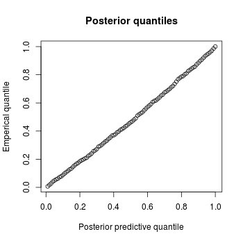
Figure 4 shows a histogram of the proportion of diseased sites for all out-of-sample posterior predictive simulations and for the observed proportions. The marginal distribution of the simulated values closely matches that for the observed values. To assess the calibration of posterior predictive distributions and their inferential accuracy, we consider the quantile of each observed value under its out-of-sample posterior predictive distribution $\phi_{ij}=\frac{1}{1000}\sum_{t=1}^{1000}\mathbbm{1}_{\{Y_{ij}<Y_{ij}^{(t)}\}}$, and compute the empirical CDF of the posterior predictive quantiles, as follows:

Figure 4 shows a plot of the empirical CDF of the posterior predictive quantiles. This is a straight line approximating the identity function, demonstrating that the predictive model is well-calibrated, and does not under-estimate or over-estimate uncertainty.

Figure 5 summarizes the posterior for the PSB model with rank$(\mathbb{B})=1$ and rank$(\mathbb{E})=1$, conditioning on the full dataset with $N=290$ individuals. Because rank$(\mathbb{B})=1$, the covariate effects can be decomposed into a single vector of weights for each covariate, for each tooth type, and for each component of the stick-breaking process. Figure 5 shows the weights for covariates and tooth types, with $95\%$ credible intervals. The covariate weights show a strong positive effect of age and a weak positive effect of smoking, a strong negative effect of sex (F) and a weak negative effect of BMI, and a negligible effect of A1C. The tooth type weights are all consistently positive, demonstrating that the effect of the covariates are similar across types, but may vary in magnitude. The conditional distribution of diseased sites across tooth types for an individual depends entirely on their univariate covariate score $XB_{1}$. Figure 5 illustrates the marginal distribution across tooth types for certain values on this continuum; for a higher covariate score, the resulting distribution favors a higher proportion of diseased sites. Thus, status is improved for females, non-smokers, younger individuals, and those with a higher BMI, and these effects are generally consistent across tooth types. The findings for sex, smoking and age are consistent with the literature on periodontal disease (Chambrone et al. 2010). The finding for BMI is somewhat counter-intuitive, and results are mixed in the literature (Kongstad et al. 2009; Chaffee and Weston 2010); an ad-hoc correlation analysis of these data similarly yields a negative correlation between BMI and proportion of diseased sites for all tooth types, with p-value$<0.01$ for canines and incisors.

Note that the use of a low-rank tensor model simplifies interpretation substantially over (e.g.) a model that allows the covariate coefficients to vary freely over different components of the PSB process and different tooth types. An online interactive visualization showing the posterior predictive distribution for proportion of diseased sites for any given tooth type and combination of individual-level predictors is available at http://ericfrazerlock.com/toothdata/ToothDisplay.html.

References

- Albert and Chib (1993) Albert, J. H. and Chib, S. (1993) Bayesian analysis of binary and polychotomous response data. Journal of the American statistical Association, 88, 669–679.
- Antoniak (1974) Antoniak, C. E. (1974) Mixtures of Dirichlet processes with applications to Bayesian nonparametric problems. The Annals of Statistics, 2, 1152–1174.
- Carroll and Chang (1970) Carroll, J. D. and Chang, J.-J. (1970) Analysis of individual differences in multidimensional scaling via an N-way generalization of “Eckart-Young” decomposition. Psychometrika, 35, 283–319.
- Carvalho et al. (2010) Carvalho, C. M., Polson, N. G. and Scott, J. G. (2010) The horseshoe estimator for sparse signals. Biometrika, 97, 465–480.
- Chaffee and Weston (2010) Chaffee, B. W. and Weston, S. J. (2010) Association between chronic periodontal disease and obesity: a systematic review and meta-analysis. Journal of periodontology, 81, 1708–1724.
- Chambrone et al. (2010) Chambrone, L., Chambrone, D., Lima, L. A. and Chambrone, L. A. (2010) Predictors of tooth loss during long-term periodontal maintenance: a systematic review of observational studies. Journal of Clinical Periodontology, 37, 675–684.
- Chung and Dunson (2009) Chung, Y. and Dunson, D. B. (2009) Nonparametric Bayes conditional distribution modeling with variable selection. Journal of the American Statistical Association, 104, 1646–1660.
- Fernandes et al. (2009) Fernandes, J. K., Wiegand, R. E., Salinas, C. F., Grossi, S. G., Sanders, J. J., Lopes-Virella, M. F. and Slate, E. H. (2009) Periodontal disease status in Gullah African Americans with type 2 diabetes living in South Carolina. Journal of Periodontology, 80, 1062–1068.
- Geoffrey and Peel (2000) Geoffrey, M. and Peel, D. (2000) Finite Mixture Models. NJ: John Wiley & Sons, Inc.
- Gopalan and Berry (1998) Gopalan, R. and Berry, D. A. (1998) Bayesian multiple comparisons using Dirichlet process priors. Journal of the American Statistical Association, 93, 1130–1139.
- Griffin and Steel (2006) Griffin, J. E. and Steel, M. J. (2006) Order-based dependent Dirichlet processes. Journal of the American statistical Association, 101, 179–194.
- Guhaniyogi et al. (2017) Guhaniyogi, R., Qamar, S. and Dunson, D. B. (2017) Bayesian tensor regression. Journal of Machine Learning Research, 18, 1–31.
- Ishwaran and James (2001) Ishwaran, H. and James, L. F. (2001) Gibbs sampling methods for stick-breaking priors. Journal of the American Statistical Association, 96, 161–173.
- Ishwaran et al. (2005) Ishwaran, H., Rao, J. S. et al. (2005) Spike and slab variable selection: frequentist and Bayesian strategies. The Annals of Statistics, 33, 730–773.
- Johndrow et al. (2017) Johndrow, J. E., Bhattacharya, A., Dunson, D. B. et al. (2017) Tensor decompositions and sparse log-linear models. The Annals of Statistics, 45, 1–38.
- Kolda and Bader (2009) Kolda, T. G. and Bader, B. W. (2009) Tensor decompositions and applications. SIAM review, 51, 455–500.
- Kongstad et al. (2009) Kongstad, J., Hvidtfeldt, U. A., Grønbæk, M., Stoltze, K. and Holmstrup, P. (2009) The relationship between body mass index and periodontitis in the Copenhagen City Heart Study. Journal of periodontology, 80, 1246–1253.
- Lai et al. (2018) Lai, Y., Ping, Y., Xiao, K., Hao, B. and Zhang, X. (2018) Variational Bayesian inference for a Dirichlet process mixture of beta distributions and application. Neurocomputing, 278, 23–33.
- Lindley and Smith (1972) Lindley, D. V. and Smith, A. F. (1972) Bayes estimates for the linear model. Journal of the Royal Statistical Society. Series B (Methodological), 1–41.
- Lock (2018) Lock, E. F. (2018) Tensor-on-tensor regression. Journal of Computational and Graphical Statistics, 27, 638–647.
- Lock and Dunson (2017) Lock, E. F. and Dunson, D. B. (2017) Bayesian genome-and epigenome-wide association studies with gene level dependence. Biometrics, 73, 1018–1028.
- MacEachern (2000) MacEachern, S. N. (2000) Dependent Dirichlet processes. Unpublished manuscript, 1–40.
- MacEachern and Müller (1998) MacEachern, S. N. and Müller, P. (1998) Estimating mixture of Dirichlet process models. Journal of Computational and Graphical Statistics, 7, 223–238.
- Rodriguez and Dunson (2011) Rodriguez, A. and Dunson, D. B. (2011) Nonparametric Bayesian models through probit stick-breaking processes. Bayesian analysis (Online), 6.
- Sethuraman (1994) Sethuraman, J. (1994) A constructive definition of Dirichlet priors. Statistica Sinica, 4, 639–650.
- Wei and Li (2011) Wei, X. and Li, C. (2011) The Student’s -hidden Markov model with truncated stick-breaking priors. IEEE Signal Processing Letters, 18, 355–358.
- Wei and Li (2012) — (2012) The infinite Student’s -mixture for robust modeling. Signal Processing, 92, 224–234.
- Zhou et al. (2015) Zhou, J., Bhattacharya, A., Herring, A. H. and Dunson, D. B. (2015) Bayesian factorizations of big sparse tensors. Journal of the American Statistical Association, 110, 1562–1576.
Appendix A Gibbs sampling algorithm
The Gibbs sampling algorithm for the full model given in Figure 2, using the parameter augmentation described in Section 3, proceeds as follows:
- 1.
Update ’s, where
- 2.
Update the atoms for . Let and be the total number of affected sites and total number of sites, respectively, that belong to observations allocated to DP component :
The full conditional distribution of is then
- 3.
Update the ’s:
where and define a normal distribution truncated below or above , respectively.
- 4.
Update the coefficient tensor . Define the array where . Then, where , , and defines the contracted tensor product over dimension . We sample from the full conditional distributions of , , and as in Section 8 of Lock 2018.
- 5.
Update the individual effect tensor . Define the array where . The entries of are independent and normally distributed with mean array and variance . The full conditional distributions for , and can each be found by an application of well-known results for the Bayesian linear model (Lindley and Smith 1972). For example, consider . Let the columns of be given by the outer product of the respective columns in and :
where vec is the vectorization operator. Let give the matricization of , i.e.,
Then, regresses on , giving
where is the diagonal covariance matrix with . The full conditional distributions for and are analogous to that for , but with diagonal prior covariance .
- 6.
- 7.
Update the ’s. Define the array where .
- 8.
Update : for .
- 9.
Update the stick-breaks for . For is
with .
- 10.
Update the weights for .
- 11.
Update for each pair .
- 12.
Determine component weights via