Strong vorticity fluctuations and antiferromagnetic correlations in axisymmetric fluid equilibria

The outline of the remainder of this paper is as follows. The basic equations of motion, derived from the 3D Euler equation under the axial flow assumption and reduced to a pair of coupled 2D equations for $\xi$ and $\sigma$ (defined on the poloidal plane), are summarized in Sec. II. The key conservation laws are summarized in Sec. III. In addition to the usual kinetic energy, linear momentum along the cylinder axis, and angular momentum about the axis, these include two infinite classes of conserved circulation integrals that are a consequence of the constrained effectively 2D dynamics. The first class involves $\sigma$ alone. The second couples both fields, but only linearly in $\xi$. All of the conserved values may be viewed as fixed by the flow initial condition, and then maintained through the turbulent cascade that leads to the late-time equilibrated flow.

In Sec. IV the thermodynamic free energy fully characterizing the equilibrium flows is defined in terms of the underlying grand canonical statistical mechanics formalism laid out in Apps. A and B. The continuum fluid results are obtained through a limiting procedure in which the continuous poloidal plane is replaced by a 2D grid with microscopic mesh size $a$, and the limit $a\to 0$ taken. Similar to the Euler case MWC1992, it transpires that the temperature and other model parameters must be scaled appropriately with $a$ in order to obtain a sensible thermodynamic limit. At this point the basic positive temperature requirement is an obvious consequence of the unboundedness of the poloidal field $\xi$, which is then capable of absorbing arbitrarily energies.

To gain basic intuition, in Sec. V the exact solution is derived for the special choice of parameters in which the toroidal and poloidal degrees of freedom are completely decoupled. This solution will turn out to be highly relevant to the general case as well. We also introduce a class of “finite level” models in which the full set of conserved integrals are constrained to a finite number through a special choice of parameters. These are particularly amenable to analytic and numerical solution.

In Sec. VI the full coupled model is considered, and reduced models are derived focusing separately on the toroidal and poloidal fields. In particular, by integrating out the poloidal field $\xi$, the effective theory for $\sigma$ is shown to be equivalent to a certain type of classical antiferromagnetic (AF) spin model on the microgrid. Proper scaling in the $a\to 0$ limit, however, turns out to generate only very weak antiferromagnetic correlations, allowing an exact perturbative treatment of both classes of conservation laws. The intuition here is that the bias on $\xi$ introduced by the second class of conservation laws is rather weak compared to the intrinsic microscale fluctuations, and the final result lies very close to the decoupled model solution.

On the other hand, the effective theory for $\xi$, obtained by integrating out the toroidal field $\sigma$, is that of a plasma model with long range logarithmic (2D Coulomb-type) interactions—as would be expected from the underlying vortex degrees of freedom. The AF correlations are here reflected in the strong tendency toward local charge neutrality in Coulomb systems, which includes also the classic electrostatic effect in which all uncompensated free charges are pushed to the system boundary. There they are distributed in such a way as to produce vanishing interior large scale flow (equivalent to the requirement of vanishing static electric field within a conducting body).

In Sec. VII some simple examples, including a detailed look at the two-level model, are treated and used to illustrate the general theory.

The paper is concluded in Sec. VIII. In particular, comparison is made with the approach of Ref. TDB2014 in which an artificial cutoff $|\xi|<M$ is applied, and the limit $M\to\infty$ taken after $a\to 0$. These two limits do not generally commute and this strongly impacts the physical consequences of the theory. In particular, the variational approach used there, indeed valid in parameter regimes where $|\xi|=O(M)$ is dominated by the cutoff, is seen here to fail when $|\xi|\ll M$ is finite, missing the effects of strong positive temperature fluctuations.

It follows from (2) that

$$\partial_{r}(rv_{r})+\partial_{z}(rv_{z})=0,$$

(4)

allowing one to represent

$$v_{r}=-\frac{1}{r}\partial_{z}\psi,\ \ v_{z}=\frac{1}{r}\partial_{r}\psi$$

(5)

in terms of a stream function $\psi(r,z)$. The velocity is therefore conveniently represented in the form

$${\bf v}=\nabla\times\left(\frac{1}{r}\psi\hat{\bf\theta}\right)+\frac{1}{r}\sigma\hat{\bm{\theta}}$$

(6)

in which $\psi$ and the vertical component of the angular momentum density

$$\sigma=rv_{\theta}$$

(7)

about the symmetry axis are taken as the fundamental fields.

The axial vorticity $\omega_{\theta}$ is related to the stream function by

	$\displaystyle\omega_{\theta}$	$\displaystyle\equiv$	$\displaystyle\hat{\bf z}\cdot\nabla\times{\bf v}=\partial_{z}v_{r}-\partial_{r}v_{z}$		(8)
		$\displaystyle=$	$\displaystyle-\frac{1}{r}\partial_{z}^{2}\psi-\partial_{r}\left(\frac{1}{r}\partial_{r}\psi\right).$

Defining scaled vorticity

$$\xi=\frac{\omega_{\theta}}{r},$$

(9)

and the modified radial and 2D coordinates

$$y=\frac{r^{2}}{2},\ {\bm{\rho}}=(y,z)$$

(10)

one may express the poloidal velocity components in the form

	$\displaystyle(v_{r},v_{z})$	$\displaystyle=$	$\displaystyle\left(-\frac{1}{\sqrt{2y}}\partial_{z}\psi,\partial_{y}\psi\right)\equiv\nabla_{*}\times\psi$
	$\displaystyle\nabla_{*}$	$\displaystyle\equiv$	$\displaystyle\hat{\bf y}\partial_{y}\psi+\hat{\bf z}\frac{1}{\sqrt{2y}}\partial_{z},$		(11)

and the poloidal (scaled) vorticity is given by

$$\xi=-\left(\frac{1}{2y}\partial_{z}^{2}+\partial_{y}^{2}\right)\psi\equiv-\Delta_{*}\psi.$$

(12)

For a simply connected domain, the free slip condition is enforced with Dirichlet boundary conditions, $\psi|_{\partial D}=0$. The generalized Laplace equation may be solved to derive $\psi$ from any given $\xi$:

$$\psi({\bm{\rho}})=\int_{D}d{\bm{\rho}}^{\prime}G({\bm{\rho}},{\bm{\rho}}^{\prime})\xi({\bm{\rho}})$$

(13)

with generalized Laplacian Green function obeying

$$-\Delta_{*}G({\bm{\rho}},{\bm{\rho}}^{\prime})=\delta({\bm{\rho}}-{\bm{\rho}}^{\prime}).$$

(14)

and satisfying the same Dirichlet boundary condition in both arguments.

More generally, for the multiply connected cylindrical geometry of primary interest here, free slip boundary conditions in general allow different constant values of $\psi$ on the inner and outer boundaries of the cylinder, $r_{\mathrm{in}}\leq r\leq r_{\mathrm{out}}$ W2017. This may be handled by accounting for the mean vertical flow

$$v_{z}^{0}=\frac{1}{V_{\cal D}}\int_{\cal D}d{\bf x}v_{z}$$

(15)

in which $V_{\cal D}=\pi h(r_{\mathrm{out}}^{2}-r_{\mathrm{in}}^{2})=2\pi h(y_{\mathrm{out}}-y_{\mathrm{in}})$ is the cylinder volume, with $h$ its height. Conservation of vertical momentum implies that $v_{z}^{0}$ is a constant of the motion (see Sec. III.3), and the subtracted stream function

$$\psi_{D}=\psi-v_{z}^{0}y,\$$

(16)

may be chosen to vanish on both boundaries. The scaled vorticity remains unchanged,

$${\bf v}_{D}={\bf v}-v_{z}^{0}\hat{\bf z}\ \Rightarrow\ \xi=-\Delta_{*}\psi_{D}$$

(17)

and (13) therefore generalizes to

	$\displaystyle\psi({\bm{\rho}})$	$\displaystyle=$	$\displaystyle\psi_{D}({\bm{\rho}})+v_{z}^{0}y$		(18)
		$\displaystyle=$	$\displaystyle\int_{D}d{\bm{\rho}}^{\prime}G({\bm{\rho}},{\bm{\rho}}^{\prime})\xi({\bm{\rho}})+v_{z}^{0}y$

in which $v_{z}^{0}$ is a fixed parameter defined, e.g., by the flow initial condition.

The azimuthal component of the Euler equation takes the form

$$\partial_{t}v_{\theta}+v_{r}\partial_{r}v_{\theta}+v_{z}\partial_{z}v_{\theta}+\frac{v_{\theta}v_{r}}{r}=0,$$

(19)

which reduces to

$$\partial_{t}\sigma+{\bf w}\cdot\nabla_{\bm{\rho}}\sigma=0,$$

(20)

in which $\nabla_{\bm{\rho}}=(\partial_{y},\partial_{z})$ is a 2D gradient, and

$${\bf w}=\nabla_{\bm{\rho}}\times\psi=(-\partial_{z}\psi,\partial_{y}\psi)=(rv_{r},v_{z})$$

(21)

satisfies the 2D incompressibility condition

$$\nabla_{\bm{\rho}}\cdot{\bf w}=0.$$

(22)

Equation (20) expresses the fact that, in this modified 2D coordinate system, the toroidal flow parameter $\sigma$ is freely advected by the incompressible poloidal flow generated by $\xi$.

Applying appropriate spatial derivatives to the Euler equation and using the incompressibility constraint (4), the axial vorticity (8) obeys

$$\partial_{t}\omega_{\theta}+v_{r}\partial_{r}\omega_{\theta}+v_{z}\partial_{z}\omega_{\theta}-\frac{\omega_{\theta}v_{r}}{r}=\frac{\partial_{z}v_{\theta}^{2}}{r},$$

(23)

which may be put in the form

$$\partial_{t}\xi+{\bf w}\cdot\nabla_{\bm{\rho}}\xi=\frac{\partial_{z}\sigma^{2}}{4y^{2}}.$$

(24)

Thus, 2D advection of $\xi$ (by its self-generated poloidal flow field) is forced by $\sigma$.

Equations (20) and (24) are the fundamental equations of motion for axisymmetric flow, reducing the 3D vector Euler equation (1) to a pair of coupled 2D scalar equations. The original 3D velocity field is recovered using (7), and by constructing the 2D stream function (18), and then using (5) in conjunction with the coordinate mapping (10).

The kinetic energy is

	$\displaystyle E$	$\displaystyle=$	$\displaystyle\frac{1}{2}\int_{\cal D}d{\bf x}|{\bf v}|^{2}=\frac{1}{2}\int_{\cal D}d{\bf x}\left[|{\bf v}_{D}|^{2}+(v_{z}^{0})^{2}\right]$		(25)
		$\displaystyle=$	$\displaystyle\pi\int_{D}d{\bm{\rho}}\left[|\nabla_{*}\psi_{D}|^{2}+\frac{\sigma^{2}}{2y}\right]+E_{z}^{0}$
		$\displaystyle=$	$\displaystyle\pi\int d{\bm{\rho}}\left(\xi\psi_{D}+\frac{\sigma^{2}}{2y}\right)+E_{z}^{0}$
		$\displaystyle=$	$\displaystyle E_{G}[\xi]+\pi\int d{\bm{\rho}}\frac{\sigma^{2}}{2y}+E_{z}^{0}$

in which

	$\displaystyle E_{z}^{0}$	$\displaystyle=$	$\displaystyle\frac{1}{2}V_{\cal D}(v_{z}^{0})^{2}$
	$\displaystyle E_{G}[\xi]$	$\displaystyle=$	$\displaystyle\pi\int_{D}d{\bm{\rho}}\int_{D}d{\bm{\rho}}^{\prime}\xi({\bm{\rho}})G({\bm{\rho}},{\bm{\rho}}^{\prime})\xi({\bm{\rho}}^{\prime})$		(26)

are the kinetic energies associated, respectively, with the mean and poloidal flows. To derive the latter, equation (18) has been used following an integration by parts. The surface term vanishes by virtue of the ability to impose $\psi_{D}|_{\partial D}=0$.

Energy conservation (which does not require axisymmetry) is verified by noting that, using the Euler equation (1) and the incompressibility condition (2), the equation of motion for the kinetic energy density

$$\varepsilon=\frac{1}{2}|{\bf v}|^{2}$$

(27)

takes the form of the conservation law

$$\partial_{t}\varepsilon+\nabla\cdot{\bf j}_{\varepsilon}=0$$

(28)

with energy current

$${\bf j}_{\varepsilon}=(p+\varepsilon){\bf v}.$$

(29)

It follows that

	$\displaystyle\partial_{t}E$	$\displaystyle=$	$\displaystyle-\int_{\cal D}d{\bf x}\nabla\cdot{\bf j}_{\varepsilon}$		(30)
		$\displaystyle=$	$\displaystyle-\int_{\partial{\cal D}}dA(p+\varepsilon){\bf v}\cdot\hat{\bf n}=0.$

The surface integral over the boundary $\partial{\cal D}$ vanishes for any combination of periodic and free slip boundary conditions (${\bf v}\cdot\hat{\bf n}=0$).

It follows from (20) and (22) that any function $f(\sigma)$ obeys the conservation law

$$\partial_{t}f(\sigma)+\nabla_{\bm{\rho}}\cdot[f(\sigma){\bf w}]=0$$

(31)

The vorticity integral

$$\Omega_{f}=\pi\int_{D}d{\bm{\rho}}f(\sigma)$$

(32)

then obeys

	$\displaystyle\partial_{t}\Omega_{f}$	$\displaystyle=$	$\displaystyle-\pi\int_{D}d{\bm{\rho}}\nabla_{\bm{\rho}}\cdot[f(\sigma){\bf w}]$		(33)
		$\displaystyle=$	$\displaystyle-\pi\int_{\partial D}dlf(\sigma){\bf w}\cdot\hat{\bf n}=0$

Here, we make use of the fact that the free slip boundary condition is equivalent to ${\bf w}\cdot\hat{\bf n}=0$ in the modified coordinates, and is valid for arbitrary $D$. The special case $f(\sigma)=\sigma$ coincides with conservation of total angular momentum about the symmetry axis.

More generally, from (20), (22) and (24) the combination $\xi f(\sigma)$ obeys

$$\partial_{t}[\xi f(\sigma)]+\nabla_{\bm{\rho}}\cdot[\xi f(\sigma){\bf w}]=\frac{f(\sigma)\partial_{z}\sigma^{2}}{4y^{2}}$$

(34)

from which follows the conservation law form

$$\partial_{t}[\xi f(\sigma)]+\nabla_{\bm{\rho}}\cdot\left[\xi f(\sigma){\bf w}+\frac{F(\sigma)}{4y^{2}}\hat{\bf z}\right]=0$$

(35)

in which $F(\sigma)$ obeys

$$F^{\prime}(\sigma)=2\sigma f(\sigma)\ \Rightarrow\ F(\sigma)=2\int_{0}^{\sigma}sf(s)ds.$$

(36)

The integral

$$\tilde{\Omega}_{f}=\pi\int_{D}d{\bm{\rho}}\xi f(\sigma)$$

(37)

therefore obeys

$\displaystyle\partial_{t}\tilde{\Omega}_{f}$

$\displaystyle=$

$\displaystyle-\pi\int_{\partial D}dl\frac{F(\sigma)}{4y^{2}}\hat{\bf z}\cdot\hat{\bf n}$

(38)

which vanishes for a cylindrical boundary $r_{\mathrm{in}}\leq r\leq r_{\mathrm{out}}$ (enforcing $\hat{\bf z}\cdot\hat{\bf n}=0$) along with periodic boundary conditions in $0\leq z<h$.

The interpretation here is that in addition to being self-advected by ${\bf w}$, the axial vorticity $\xi$ is advected vertically by the angular momentum density $\sigma$. Hence, only for a vertical boundary does the net advection keep $\xi$ from effectively exiting or entering the domain.

As illustrated in Fig. 2, the full infinite set of conserved vorticity integrals may be conveniently parameterized by the functionals

	$\displaystyle\gamma[\sigma](s)$	$\displaystyle=$	$\displaystyle\int_{D}d{\bm{\rho}}\delta[s-\sigma({\bm{\rho}})]$
	$\displaystyle\tilde{\gamma}[\xi,\sigma](s)$	$\displaystyle=$	$\displaystyle\int_{D}d{\bm{\rho}}\xi({\bm{\rho}})\delta[s-\sigma({\bm{\rho}})]$		(39)

which measure, for each real value $-\infty<s<\infty$, the fractional area on which $\sigma$ takes the value $s$, in the second case weighted by the values of $\xi$. Given these functions, one directly derives for any function $f$,

	$\displaystyle\Omega_{f}[\sigma]$	$\displaystyle=$	$\displaystyle\int ds\gamma[\sigma](s)f(s)$
	$\displaystyle\tilde{\Omega}_{f}[\xi,\sigma]$	$\displaystyle=$	$\displaystyle\int ds\tilde{\gamma}[\xi,\sigma](s)f(s).$		(40)

As alluded to below (15), for the case of cylindrical boundary, translation symmetry in $z$ implies conservation of vertical momentum

$$P_{z}=\int_{\cal D}d{\bf x}v_{z}=V_{\cal D}v_{z}^{0},$$

(41)

with or without axisymmetry. To verify this formally, the $z$-component of (1) may be written in the form

$$\partial_{t}v_{z}+\nabla\cdot{\bf j}_{z}=0,\ \ {\bf j}_{z}\equiv v_{z}{\bf v}+p\hat{\bf z},$$

(42)

and it follows that

$$\partial_{t}P_{z}=-\int_{\partial D}dA(v_{z}{\bf v}+p\hat{\bf z})\cdot\hat{\bf n}=0$$

(43)

for free slip boundary conditions on a cylinder.

From (5) it follows more explicitly that

$$P_{z}=2\pi h[\psi(r_{\mathrm{out}})-\psi(r_{\mathrm{in}})]$$

(44)

is completely determined by the Dirichlet boundary conditions on $\psi$. In particular, as claimed earlier, $P_{z}=0$ may be enforced by setting $\psi=0$ on both boundaries.

Using the square grid discretization (134) foot:gridunits, the statistics of the $\sigma$ field are clearly decoupled from site to site, and one obtains

$$Z_{\sigma}=\prod_{l}Z_{1}[\beta a^{2},\mu,y_{l}]$$

(50)

with factor $a^{2}$ coming from the discretization of $\int_{D}d{\bm{\rho}}$, the product extending over all lattice sites, and single site partition function

$$Z_{1}(\bar{\beta},\mu,y)=\int dse^{-\bar{\beta}\left[\frac{\pi s^{2}}{2y}-\mu(s)\right]}.$$

(51)

Typically, the flow initial condition will have bounded $\sigma$, hence $\gamma[\sigma](s)$ has compact support, and so therefore will $e^{-\bar{\beta}\mu(s)}$. Thus, (51) is strongly convergent for any real $\bar{\beta}$, both positive and negative. The single site probability distribution takes the form

$$p_{\sigma}(s,y)=\langle\delta[s-\sigma({\bm{\rho}})]\rangle=\frac{e^{-\beta a^{2}\left[\frac{\pi s^{2}}{2y}-\mu(s)\right]}}{Z_{1}(\beta a^{2},\mu,y)},$$

(52)

and the position-dependent mean is

$$\langle\sigma({\bm{\rho}})\rangle=\int sdsp_{\sigma}(s,y).$$

(53)

Equation (48) serves to illustrate another key result. It is seen that the properly scaled thermal variable is

$$\bar{\beta}=\beta a^{2}\ \Rightarrow\ \bar{T}=T/a^{2},$$

(54)

which needs to remain finite in the continuum limit $a\to 0$ MWC1992. Only for finite $\bar{\beta}$ does $\sigma$ have a nontrivial distribution. The $\sigma$ field free energy

	$\displaystyle F_{\sigma}(\bar{\beta},\mu)$	$\displaystyle=$	$\displaystyle-\lim_{a\to 0}\frac{1}{\beta}\ln(Z_{\sigma})$		(55)
		$\displaystyle=$	$\displaystyle-\frac{1}{\bar{\beta}}\int_{D}d{\bm{\rho}}\ln[Z_{1}(\bar{\beta},\mu,y)]\ \ \ \ \$

is also finite in the continuum limit. The latter corresponds to the thermodynamic limit in the sense that the number of grid cells $V_{\cal D}/\pi a^{2}$ diverges. For cylindrical ${\cal D}$ this expression may clearly be simplified, but in this section we treat this as a special case of the more general domain.

Finite $\beta$, on the other hand, leads to $\bar{\beta}=\beta/a^{2}\to\infty$ and $\bar{T}=Ta^{2}\to 0$. The zero temperature limit leads to frozen $\sigma=s_{0}(y)$ at the value $s_{0}$ minimizing ($\beta>0$) or maximizing ($\beta<0$) the exponent $\frac{\pi s^{2}}{2y}-\mu(s)$ over the support of $\mu$. More generally, positive temperatures encourage larger $\sigma$ values to gather at smaller radii (larger $1/2y$), while negative temperatures encourage them to gather at larger radii (smaller $1/2y$) TDB2014.

The constraint equation (154) for the conserved integral $g(s)$ takes the explicit form

$$g(s)=-\frac{\delta F_{\sigma}}{\delta\mu(s)}=\int_{D}d{\bm{\rho}}p_{\sigma}(s,y)$$

(56)

Using independence of the two fields in the decoupled model, one obtains trivially

	$\displaystyle\tilde{g}(s)$	$\displaystyle=$	$\displaystyle\int_{D}d{\bm{\rho}}\langle\xi({\bm{\rho}})\delta[s-\sigma({\bm{\rho}})]\rangle$		(57)
		$\displaystyle=$	$\displaystyle\int_{D}d{\bm{\rho}}\langle\xi({\bm{\rho}})\rangle p_{\sigma}(s,y)$
		$\displaystyle\equiv$	$\displaystyle 0$

since $E_{G}[\xi]$ is a positive even functional of $\xi$.

A common approximation is to restrict the initial condition for $\sigma$ to a finite, discrete set of levels. As the simplest model, which will form the basis for most explicit examples in later sections, the two level system is described by

$$g(s)=A_{D}[p_{1}\delta(s-s_{1})+p_{2}\delta(s-s_{2})]$$

(58)

with, by convention, $s_{2}>s_{1}$, and in which $A_{D}=\int_{D}d{\bm{\rho}}=V_{\cal D}/2\pi$ is the modified coordinate area of $D$, and $p_{1},p_{2}=1-p_{1}$ are, respectively, the fractional areas on which $\sigma({\bm{\rho}})=s_{1},s_{2}$. The corresponding chemical potential must take the general form

$$e^{\bar{\beta}\mu(s)}=e^{\bar{\beta}\mu_{1}}\delta(s-s_{1})+e^{\bar{\beta}\mu_{2}}\delta(s-s_{2}),$$

(59)

which leads to

	$\displaystyle Z_{1}$	$\displaystyle=$	$\displaystyle e^{\bar{\beta}(\mu_{1}-\pi s_{1}^{2}/2y)}+e^{\bar{\beta}(\mu_{2}-\pi s_{2}^{2}/2y)}$
	$\displaystyle p_{\sigma}(s_{1},y)$	$\displaystyle=$	$\displaystyle 1-p_{\sigma}(s_{2},y)$
		$\displaystyle=$	$\displaystyle\frac{e^{\bar{\beta}[\pi(s_{2}^{2}-s_{1}^{2})/4y-\mu_{\Delta}]}}{2\cosh\{\bar{\beta}[\pi(s_{2}^{2}-s_{1}^{2})/4y-\mu_{\Delta}]\}}$
	$\displaystyle\langle\sigma({\bm{\rho}})\rangle$	$\displaystyle=$	$\displaystyle s_{1}p_{\sigma}(s_{1},y)+s_{2}p_{\sigma}(s_{2},y)$
	$\displaystyle F_{\sigma}$	$\displaystyle=$	$\displaystyle\frac{\pi(s_{1}^{2}+s_{2}^{2})}{4}I_{D}-\mu_{0}A_{D}$		(60)
		$\displaystyle-$	$\displaystyle\frac{1}{\bar{\beta}}\int_{D}d{\bm{\rho}}\ln\left(2\cosh\left\{\bar{\beta}\left[\frac{\pi(s_{2}^{2}-s_{1}^{2})}{4y}-\mu_{\Delta}\right]\right\}\right)$

in which we define the mean and difference chemical potentials

$$\mu_{0}=\frac{\mu_{2}+\mu_{1}}{2},\ \ \mu_{\Delta}=\frac{\mu_{2}-\mu_{1}}{2}$$

(61)

and the integration constant

$$I_{D}=\int_{D}\frac{d{\bm{\rho}}}{y}.$$

(62)

The constraint equation (56) takes the form

$$p_{1}=1-p_{2}=\frac{1}{2A_{D}}\int d{\bm{\rho}}p_{\sigma}(s_{1},y).$$

(63)

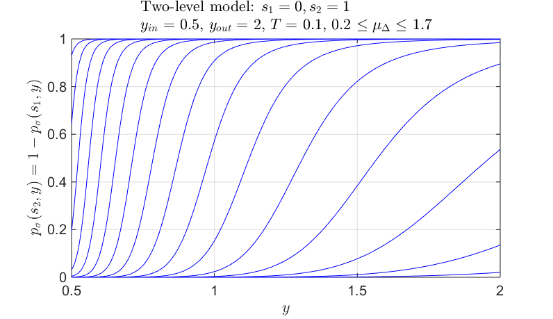
These depend only on the difference $\mu_{\Delta}$, which is then used to set the values of $p_{1,2}$. The correspondence is easily seen to be one-to-one and invertible. Some model results are plotted in Fig. 3. For example, at low temperatures it is seen that there is sharp (Fermi surface-like) interface between the smaller of $|s_{1}|,|s_{2}|$ ($y<y_{I}$) and the larger of $|s_{1}|,|s_{2}|$ ($y>y_{I}$) dominated regions, with position $y_{I}=\pi(s_{2}^{2}-s_{1}^{2})/4\mu_{\Delta}$ controlled by $\mu_{\Delta}$.

The more general $L$-level model, which restricts $\sigma({\bm{\rho}})$ to a discrete set of values $s_{1}<s_{2}<\ldots<s_{L}$, is described by

	$\displaystyle g(s)$	$\displaystyle=$	$\displaystyle A_{D}\sum_{m=1}^{L}p_{m}\delta(s-s_{m}),\ \sum_{m=1}^{L}p_{m}=1$
	$\displaystyle e^{\bar{\beta}\mu(s)}$	$\displaystyle=$	$\displaystyle\sum_{m=1}^{L}e^{\bar{\beta}\mu_{m}}\delta(s-s_{m})$		(64)

which leads to

	$\displaystyle Z_{1}$	$\displaystyle=$	$\displaystyle\sum_{m=1}^{L}e^{-\bar{\beta}\pi s_{m}^{2}/2y}e^{\bar{\beta}\mu_{m}}$
	$\displaystyle F_{\sigma}$	$\displaystyle=$	$\displaystyle-\frac{1}{\bar{\beta}}\int_{D}d{\bm{\rho}}\ln\left(\sum_{m=1}^{L}e^{\bar{\beta}\mu_{m}}e^{-\bar{\beta}\pi s_{m}^{2}/2y}\right).$		(65)

Defining $m_{0}=\arg\min\{|s_{m}|\}$ (the index of the smallest magnitude $|s_{m}|$), the constraint equations may be put in the form

	$\displaystyle p_{m}$	$\displaystyle=$	$\displaystyle\frac{1}{A_{D}}\int_{D}d{\bm{\rho}}p_{\sigma}(s_{m},y)$		(66)
	$\displaystyle p_{\sigma}(s_{m},y)$	$\displaystyle=$	$\displaystyle\frac{e^{\bar{\beta}\Delta\mu_{m}}e^{-\bar{\beta}\pi(s_{m}^{2}-s_{m_{0}}^{2})/2y}}{1+\sum_{m^{\prime}\neq m_{0}}^{L}e^{\bar{\beta}\Delta\mu_{m^{\prime}}}e^{-\bar{\beta}\pi(s_{m^{\prime}}^{2}-s_{m_{0}}^{2})/2y}},$

with the differences $\Delta\mu_{m}=\mu_{m}-\mu_{m_{0}}$, $m\neq m_{0}$, used to set the $L-1$ independent $p_{m}$ values. The areas $A_{m}=A_{D}p_{m}$ on which $\sigma=s_{m}$ are conserved by the flow, though the corresponding domain geometries strongly mix at ever finer scales as time advances.

Analogous to the result for the two-level model, each difference $\Delta\mu_{m}$ controls the position of an interface, at position $y_{m}=(s_{m}^{2}-s_{m_{0}}^{2})/2\Delta\mu_{m}$, separating $s_{m}$-present ($y>y_{m}$) and $s_{m}$-absent ($y<y_{m}$) regions.

Since $E_{G}[\xi]$ is positive definite, (45) makes sense only for positive temperatures, $\beta>0$. This is in contrast to the Euler equation M1990; MWC1992, where the equivalent of the field $\xi$ is directly constrained by the conservation laws, and negative temperature equilibria are ubiquitous.

In order to verify that the combination $\bar{\beta}$ is appropriate here as well, consider the square grid Gaussian form

$$e^{-\beta E_{G}[\xi]}=e^{-\frac{1}{2}\sum_{l,m}A_{lm}\xi_{l}\xi_{m}}$$

(67)

with discrete variables

	$\displaystyle\xi_{l}$	$\displaystyle=$	$\displaystyle\xi({\bm{\rho}}_{l})$
	$\displaystyle A_{lm}$	$\displaystyle=$	$\displaystyle\bar{\beta}a^{2}G({\bm{\rho}}_{l},{\bm{\rho}}_{m}).$		(68)

The discrete approximation to the Green function equation (14) takes the form

$$-\sum_{n}\Delta_{ln}G({\bm{\rho}}_{n},{\bm{\rho}}_{m})=\delta_{lm}$$

(69)

in which

	$\displaystyle\Delta_{lm}$	$\displaystyle=$	$\displaystyle a^{2}[\Delta_{*}]_{lm}$		(70)
		$\displaystyle=$	$\displaystyle\delta_{l+\hat{\bf y},m}-2\delta_{lm}+\delta_{l-\hat{\bf y},m}$
			$\displaystyle+\ \frac{\delta_{l+\hat{\bf z},m}-2\delta_{lm}+\delta_{l-\hat{\bf z},m}}{2y_{l}}$

is the discrete (nearest neighbor finite difference) version of the generalized Laplacian. The Dirichlet boundary conditions on $G$ lead to the vanishing of (69) when either or both $l,m$ lie on the boundary, hence (69) only makes sense if both indices $l,m$ correspond to interior points of $D$. Thus, all terms in (70) vanish if $l$ itself is a boundary point; and if $l$ is an interior point, the corresponding nearest neighbor Kronecker delta is absent if $l+\hat{\bm{\delta}}$ is a boundary point (with $\hat{\bm{\delta}}$ any of the four nearest neighbor directions).

Put another way, from the fact that boundary values of $\xi$ do not contribute to $E_{G}$ it follows that $\sum_{m}G_{lm}\xi_{m}\equiv 0$ for any $\xi$ entirely supported on the boundary. Thus, the matrix $G$ is not invertible unless restricted to the interior. It follows also that, in order to obtain a finite well defined free energy, the functional integral over $\xi$ must be restricted to interior points as well. Note that since the $\sigma$ field is strongly regularized, whether or not one includes values on the boundary is of negligible consequence in the continuum limit, but for consistency we will restrict it to interior sites as well.

References

- (1) J. Miller, “Statistical mechanics of euler equations in two dimensions,” Phys. Rev. Lett. 65, 2137 (1990).
- (2) R. Robert and J. Sommeria, J. Fluid Mech. 229, 291 (1991).
- (3) J. Miller, P. B. Weichman, and M. C. Cross, “Statistical mechanics, Euler’s equation, and Jupiter’s Red Spot,” Phys. Rev. A 45, 2328 (1992).
- (4) A. Renaud, A. Venaille, and F. Bouchet, “Equilibrium statistical mechanics and energy partition for the shallow water model,” J. Stat. Phys. 163, 784–843 (2016)
- (5) Notably, a mathematically equivalent theory of galaxy dynamics (based on the Boltzmann equation) was derived much earlier: D. Lynden-Bell, “Statistical Mechanics of Violent Relaxation in Stellar Systems,” Mon. Not. R. Astron. Soc. 136, 101 (1967). However, these results failed to transition to the fluid dynamics community.
- (6) L. Onsager, “Statistical hydrodynamics,” Nuovo Cimento Suppl. 6, 279 (1949).
- (7) R. H. Kraichnan, “Statistical dynamics of two-dimensional flow,” J. Fluid Mech. 67, 155 (1975).
- (8) D. Montgomery and G. Joyce, “Statistical mechanics of “negative temperature” states,” Phys. Fluids 17, 1139 (1974).
- (9) T. S. Lundgren and Y. B. Pointin, “Statistical mechanics of two-dimensional vortices,” J. Stat. Phys. 17, 323 (1977); “Non-Gaussian probability distributions for a vortex fluid,” Phys. Fluids 20, 356 (1977).
- (10) J. Michel and R. Robert, “Statistical mechanical theory of the Great Red Spot of Jupiter.” J. Stat. Phys. 77, 645 (1994).
- (11) “Emergence of intense jets and Jupiter’s Great Red Spot as maximum-entropy structures,” J. Fluid Mech. 464, 165 (2002).
- (12) P. B. Weichman, “Equilibrium theory of coherent vortex and zonal jet formation in a system of nonlinear Rossby waves,” Phys. Rev. E 73, 036313 (2006).
- (13) D. D. Holm, J. E. Marsden, T. Ratiu, and A. Weinstein, “Nonlinear stability of fluid and plasma equilibria,” Phys. Rep. 123, 1 (1985).
- (14) R. Jordan and B. Turkington, “Ideal magnetofluid turbulence in two dimensions,” J. Stat. Phys. 87, 661 (1997).
- (15) P. B. Weichman, “Long-Range Correlations and Coherent Structures in Magnetohydrodynamic Equilibria,” Phys. Rev. Lett. 109, 235002 (2012).
- (16) P. B. Weichman and D. M. Petrich, “Statistical Equilibrium Solutions of the Shallow Water Equations,” Phys. Rev. Lett. 86, 1761–64 (2001).
- (17) P. H. Chavanis and J. Sommeria, “Statistical mechanics of the shallow water system,” Phys. Rev. E 65, 026302 (2002).
- (18) P. B. Weichman, “Competing turbulent cascades and eddy–wave interactions in shallow water equilibria,” Phys. Rev. Fluids 2, 034701 (2017).
- (19) For a recent review, see: F. Bouchet and A. Venaille, “Statistical mechanics of two-dimensional and geophysical flows,” Phys. Rep. 515, 227 (2012).
- (20) S. Thalabard, B. Dubrulle, and F. Bouchet, “Statistical mechanics of the 3D axisymmetric Euler equations in a Taylor–Couette geometry,” J. Stat. Mech.: Theory and Experiment 1, P01005 (2014).
- (21) Strictly speaking, the and coordinates have different units, and a square mesh does not actually make sense. One should instead use an rectangular mesh, or first rescale to dimensionless coordinates, e.g., , . However, the statistical formalism used here relies only on periodicity of the mesh. So, for simplicity, and with a slight abuse of notation, we do not make this distinction here.
- (22) Equation (76) is the s-wave () case of the Coulomb wave equation: see p. 538 of M. Abramovitz and I. A. Stegun, Handbook of Mathematical Functions (Dover, New York, 1970).
- (23) Conversely, in the presence of true antiferromagnetic order, which would be expected for divergent coupling, , and even for sufficiently large when , the equilibrium average will display finite differences between microscale neighboring sites. Hence, noting the scaling (68) of the Laplacian, both sides of (98) will display divergent neighboring site difference. It follows that displays (divergent) antiferromagnetic order whenever does, scaling as . For this is larger than the fluctuation scale of , which does not make physical sense.
- (24) It follows from (99) that, even in the presence of antiferromagnetic order, one has , though the scaled equilibrium stream function directly tracks the antiferromagnetic structure in . For , this produces divergent microscale circulating velocity, scaling as , hence unphysically infinite kinetic energy.
- (25) More accurately, the homogeneous 2D Ising antiferromagnet, with fixed (i.e., no dependence on ), undergoes a phase transition at a temperature . If one now allows inhomogeneous , then at sufficiently high temperature, , the entire domain will be in the disordered phase, while for sufficiently low temperature, , it will be in the antiferromagnetically ordered phase. In between these two temperatures, there will be a phase boundary at radial coordinate satisfying , with the system magnetically ordered for and disordered for . In the continuum limit, one is also in the adiabatic limit, and will exactly follow the local equilibrium value of the sublattice magnetization.
- (26) There is an analogous rescaling of temperature required to obtain nontrivial point vortex Euler equilibria MWC1992, again due to the now unbounded vorticity.
- (27) P. Chen and M. C. Cross, “Statistical two-vortex equilibrium and vortex merger”, Phys. Rev. E 53, R3032–R3035 (1996).
- (28) D. G. Dritschel, W. Qi, and J. B. Marston, ”On the late-time behaviour of a bounded, inviscid two-dimensional Flow,” J. Fluid Mech. 783, 1–22 (2015).
- (29) H. Lamb, “Hydrodynamics, 6th edition” (Dover Publications, New York, 1932).
- (30) G. K. Batchelor, An Introduction to Fluid Dynamics (Cambridge University Press, Great Britain, 1967).