Understanding the computational difficulty of a binary-weight perceptron and the advantage of input sparseness
Abstract
Limited precision of synaptic weights is a key aspect of both biological and hardware implementation of neural networks. To assign low-precise weights during learning is a non-trivial task, but may benefit from representing to-be-learned items using sparse code. However, the computational difficulty resulting from low weight precision and the advantage of sparse coding remain not fully understood. Here, we study a perceptron model, which associates binary (0 or 1) input patterns with desired outputs using binary (0 or 1) weights, modeling a single neuron receiving excitatory inputs. Two efficient perceptron solvers (SBPI and rBP) usually find solutions in dense solution region. We studied this dense-region-approaching process through a decimation algorithm, where every time step, marginal probabilities of unfixed weights were evaluated, then the most polarized weight was fixed at its preferred value. We compared the decimation-fixing order of weights with the dynamics of SBPI and rBP, and studied the structure of solution subspace where early-decimation-fixed weights take their fixed values. We found that in SBPI and rBP, most time steps are spent on determining values of late-decimation-fixed weights. This algorithmic difficult point may result from strong cross-correlation between late-decimation-fixed weights in , and is related to solution condensation in during decimation. Input sparseness reduces time steps that SBPI and rBP need to find solutions, due to reduction of cross-correlation between late-decimation-fixed weights. When contraint density increases across a transition point, the portion of weights whose values are difficult to determine sharply increases, signaling difficult accessibility of dense solution region. We propose that the computational difficulty of binary-weight perceptron is related to a solution condensation process during approaching the dense solution region. Our work highlights the heterogeneity of learning dynamics of weights, which may help understand axonal pruning in brain development, and inspire more efficient algorithms to train neural networks.
1 Department of Physics, Centre for Nonlinear Studies and Institute of Computational and Theoretical Studies, Hong Kong Baptist University, Kowloon Tong, Hong Kong
2 Research Centre, HKBU Institute of Research and Continuing Education, Shenzhen, China
3 Beijing Computational Science Research Center, Beijing, China
* cszhou@hkbu.edu.hk
1 Introduction
Information of neural networks is stored in synaptic weights. An important feature of the synaptic weights in nature and simple hardware implementation is low precision [1, 2, 3]. However, assigning suitable values to low-precision weights is a non-trivial task, and is known to be intractable in the worst case [4, 5]. Artificial neural networks with low-precision weights requires more epochs to train before performance convergence [6, 7]. Therefore, it is of great interest to understand where the hardness comes from and how to avoid it or use it.
Perceptron is a one-layer network that receives inputs from many neurons and gives a single output. It serves as an elementary building block of complex neural networks, and is also one of the basic structures for learning and memory [8]. It is also a powerful computational unit by itself, and has applications in, say, rule inference [9] and data compression [10]. Here we try to understand the computational difficulty induced by low weight precision by studying perceptron whose weights take binary values (0 or 1). We consider a classification task: given a set of random input patterns, we want to adjust the synaptic weights, so that the perceptron gives a desired output in response to each input pattern. A synaptic weight configuration successfully associating all these input-output pairs is a solution of the perceptron.
Methods of statistical physics imply that most solutions of binary-weight perceptron are isolated and computationally hard to find [11, 12]. In the seminal work of Ref. [13], it is shown that the weight configuration space of binary-weight perceptron has a region where solutions densely aggregate. It is believed that solutions found by algorithms usually belong to this dense solution region [13, 14], and efficient algorithms have been designed by conducting weight configurations toward the dense solution region [15, 16, 17]. This implies that the computational difficulty in solving binary-weight perceptron, if any, should emerge during the process approaching the dense solution region. This difficulty should be related to the geometry structure of solution space around the dense solution region, and has little to do with the isolated solutions. However, there is a knowledge gap about how the structure of solution space around the dense region influences algorithmic difficulty.
The “difficulty" encountered by algorithms may have two different meanings, depending on the constraint density (, with being the number of input-output pairs to be associated and being the number of synapses). First is difficult part during efficient solving. When takes small values, there exist algorithms (such as SBPI and rBP) which can efficiently (i.e., typically take sub-exponential-to- time steps) solve the problem [18, 19]. In this case, it is interesting to study what difficult part of the solving process consumes most time, and think of methods to reduce solving time. Second is exponential-time difficulty. When takes large value, close to the theoretical capacity (which means the maximal at which perceptron theoretically has solutions), there are no known efficient solvers, so that people have to wait for exponentially long time for theoretically existing solutions. In this case, it is interesting to study what nature prevents the existence of efficient solvers. As far as we know, no study has been performed to address the difficult part during efficient solving process. It has been suggested that exponential-time difficulty is related to fragmentation of dense solution region at when [20]. However, it is unknown how this fragmentation influences the dynamics of algorithms to prevent them from finding solutions.
A possible way to reduce the computational difficulty of binary-weight perceptron is to represent the to-be-classified items using sparse code in input patterns. The functional pros and cons of input sparseness has been discussed in many contexts. On the one hand, input sparseness allows algorithms to store more input-output (IO) associations into perceptron [21, 22, 23], and facilitates classification of input patterns [24]; on the other hand, input sparseness also reduces the information content of input patterns and reduces generalization performance of the trained network [25, 26]. Despite these possible cons, biological neural analogies of perceptron, such as cerebellar Purkenje cells and insectile mushroom body output neurons receive from a large number of cerebellar granule cells and Keynon cells [27, 28], which have low firing probability. Theoretically, the advantage of input sparseness for memory storage is mainly understood by calculating theoretical capacity . The result is that input sparseness increases [27, 29]. A point seldom discussed is how input sparsity influences the time steps that an algorithm uses to find a solution, in the case that the algorithm can “efficiently" (i.e., take sub-exponential-to- time steps) solve the perceptron. Suppose in the case that solutions can be efficiently found, sparser input requires more time steps to find a solution, then the biological and engineering interest of input sparseness should be significantly weakened. In this paper, we will study this point above by investigating how input sparsity influences the difficult part during efficient solving that consumes most time steps.
One possible aspect to understand the computational difficulty of binary-weight perceptron is cross-correlation of weights in solution space. Strong cross-correlation breaks Bethe-Peierls approximation [30], which supposes that the probability distribution of the value of one weight in solution space is independent of the values of the other weights. This approximation lies in the heart of belief propagation [30], which is an ingredient of or closely related to a number of efficient algorithms [19, 15, 18, 31]. From another aspect, strong cross-correlation implies that the value preferences of a large number of weights are reconfigured in response to the flipping of a single weight. This means that in a local search algorithm, many subsequent rearrangements may be needed following the modification of a single weight, which increases the difficulty to find solutions [32]. Additionally, cross-correlation may be related to the condensation of solutions [30, 33], which means that most solutions aggregate into a small number of clusters.
In this paper, we study a perceptron model in which both inputs and weights take binary values (0 or 1), modeling a single neuron receiving excitatory inputs. To address the knowledge gap between structure of solution space around dense solution region and algorithmic difficulty, we propose to study decimation process, in which weights are successively fixed. At each time step, marginal probabilities of unfixed weights are computed using belief propagation or, in small-sized systems, enumerated solutions, then the most polarized weight is fixed at its preferred value. We will show that similarly as two efficient algorithms (SBPI and rBP), decimation is also a process approaching the dense solution region, and the order of weight-fixing in decimation is comparable to the dynamics of these two efficient algorithms. Additionally, decimation is also a simpler process than SBPI and rBP, because a weight will not change its value again once gets fixed; unlike in SBPI and rBP, where the preferences of weights are changing continuously. Therefore, decimation is an ideal surrogate process of SBPI and rBP for theoretical study. We will study the cross-correlation between weights and the geometry of solution clusters in the solution subspace made up of unfixed weights during decimation, thereby getting insight into the reshaping of solution space in efficient algorithms during approaching the dense solution region. With the help of decimation process, we hope to shed light onto the links among solving dynamics in efficient algorithms, algorithmic difficulty and structure of solution space around the dense region.
This paper is organized as follows. After describing the model in Section 2, we will investigate the capacity of the model and time steps that SBPI and rBP need to obtain solutions at different input sparsities in Section 3. In Sections 4-7, we will study difficult solving part and the advantage of input sparseness with the help of decimation. In Sections 8 and 9, we will study exponential-time difficulty by investigating the case when .
2 Model
We consider a perceptron model (Fig.1a) in which a neuron receives binary inputs (), which indicates whether the th input neuron fires or not. The synaptic weights are also binary , modeling excitatory synapses. The output of the perceptron is , which takes 1 or 0 depending on whether its total synaptic input is larger than the firing threshold , where is an adjustable parameter. This neuron is then provided input patterns and desired outputs with . The task is to adjust the synaptic weights , so that for all s. The probability that take 1 is input coding level . Input becomes sparser with smaller . In our model, is fixed at a nonzero value when , so that the number of s that take 1 is of order. has equal probability to be 0 or 1.
Now let’s discuss the meaning of . For a well-trained perceptron, it can be shown that the total synaptic current average over the patterns is equal to the firing threshold up to order (see Appendix E). As larger synaptic current consumes more energy, energetic efficient perceptron should reduce firing threshold by enlarging (Fig.1b, left). Of course, if firing threshold is too low, neuron may have high spontaneous activity due to membrane or synaptic noise [34], potentially consuming more energy. However, the advantage to enlarge should be apparent as long as such spontaneous activity is rare.
The meaning of can also be interpreted in another way by noting that the neuron output , where in the latter expression form, rescales the discrete values that weights can take. This weight rescaling can increase successful rate of memory retrieval under noise (Fig.1b, right). Intuitively, because s are supposed to be independent with each other, the standard deviation of the distribution of total synaptic current over s is approximately (Appendix E), which increases with ; and the input patterns with larger (or smaller) than the firing threshold associate with output 1 (or 0). Under noise with strength , the perceptron may not give correct outputs in response to input patterns whose s lie within the range (red region in Fig.1b, right). However, when gets larger, the distribution of s becomes broader (gray curve in Fig.1b, right), so that the portion of patterns whose s lie within this range decreases, which means that perceptron is more likely to output the associated value in response to a stored input pattern under noise. We provide numeric evidence to support this intuition in Supplemental Material Section 1 and Supplementary Fig.1.
In a large body of literature (e.g. Ref. [35, 36]), retrieval robustness is realized by requiring that total synaptic input is above (below) firing threshold by a stability parameter when the desired output is active (inactive). Here we effectively set . Introducing ensures that memory retrieval is always successful when the noise strength , but enlarging increases the probability of successful retrieval when .
Together, in our model, the requirements for low energy cost and high robustness for memory retrieval can be unified in a single motivation: enlarging .
3 Computational advantage of sparse input under large
We evaluated the capability of our perceptron model in classification task by investigating two efficient algorithmic solvers: stochastic Belief-Propagation Inspired algorithm (SBPI) [18] and reinforced Belief Propagation (rBP) [19]. Both algorithms assign a hidden state to weight , update during solving, and take (or 1) when is negative (or positive), see Appendix A for more details of their implementations:
(1) SBPI is a biologically plausible on-line algorithm, in which an input-output (IO) pair is presented at each time step. If the presented IO pair is unassociated (i.e., when but or when but ), then hidden state is updated as , so that may be flipped towards the direction that facilitates the association of the presented IO pair. If and the presented IO pair is associated, but the synaptic current is too close to the firing threshold , or in other words, the presented IO pair is just on the edge of association, then is also updated, with some probability, as , to increase the margin between and .
(2) rBP is a message-passing algorithm, which uses belief propagation (BP) to update . Specifically,
| (1) |
| (2) |
| (3) |
In the equations above, and are BP update functions, is the BP estimate of single-site field, is a random number that takes with probability and 0 otherwise, and is a damping factor. The meaning of eqs.1-3 is to use BP to evaluate single-site field , and then in the next time step, with probability add as an external field to BP.
We first studied the dependence of algorithmic capacity of SBPI and rBP on and . means the maximal number of IO pairs that the perceptron can associate using an algorithm. We found that at a given , increases with when is smaller than an optimal value , and decreases with when (Fig.2a-c). So this , which decreases with (Fig.2a-c), divides the function of with into two branches: low- and high- branches. Because of the non-monotonicity of with , an usually corresponds with two values at a given (Fig.2a-c). However, biologically and engineeringly good design should choose to work at the larger value, because it implies lower energy cost or higher retrieval robustness without compromising memory capacity. So only the high- branch is of biological and engineering interest, and will be considered in the following discussion. At a given , the dependence of on may not be monotonic, but if we only look at high- branch, increases with input sparseness (Fig.2a-c). This means that under the requirements of low energy consumption and robust memory retrieval, input sparseness facilitates memory capacity. From another aspect, the decrease of with at high- branch reflects the competition between capacity with energy cost or retrieval robustness, but this competition can be alleviated by increasing input sparseness: decreasing enables the same to be fulfilled using a larger (Fig.2a-c).
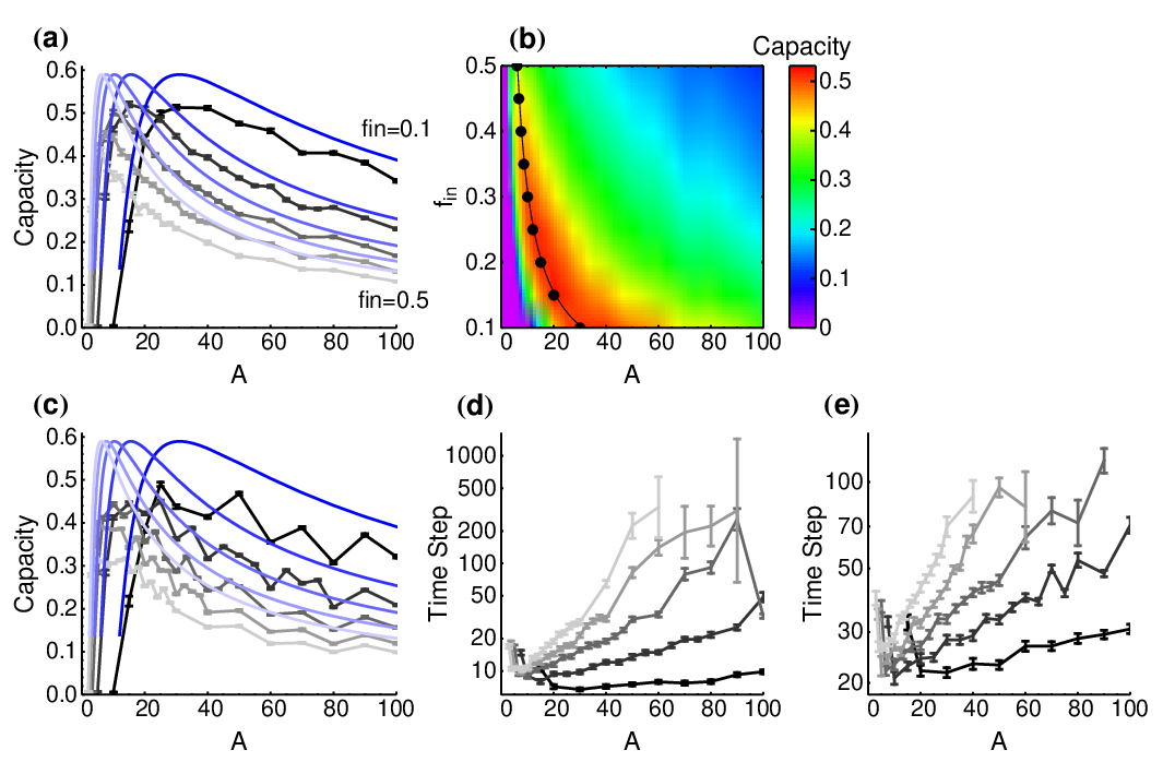
To understand the change of with and , we first calculated theoretical capacity using replica method (Appendix E), which means the maximal number of IO pairs that perceptron has a solution, and provides an upper bound of . We found that the change of with and follows similar profile as (Fig.2a,c): the function of with also has two branches; and at high- branch, increases with . We discuss the non-monotonicity of capacity with and in Supplemental Material Section 2 and Supplementary Fig.2, and we find that the existence of low- branch is because of the upper boundedness of weights (i.e., ) in our model.
However, only calculating is not sufficient to understand the computational advantage of input sparseness, because it is possible that algorithms need more time steps to find a solution even though there are more solutions in the weight configuration space. How easy it is to get solutions also matters: on the one hand, algorithms usually have a upper limit of time step , and only the cases when solutions are found within time steps report solving success and contribute to ; on the other hand, solving perceptron in less time steps, which implies quick learning, is itself of biological and engineering interest.
We investigated the time steps that SBPI and rBP use to solve under different input sparsities at a given . Under SBPI, the change of with and is largely anti-correlated with the change of : the function of with also has two branches, and at high- branch, decreases with input sparseness (Fig.2d). Under rBP, however, the change of with is more subtle, dependent on the parameter of rBP. At the high- branch of , at a fixed , may not decrease with input sparseness (Supplementary Fig.3b); but if we also tune , defining as the minimal time steps that rBP achieves successful solving under different s, then follows similar profile as that in SBPI (Fig.2e): has two branches with , and decreases with input sparseness at high- branch. This means that we are, in principle, able to design a new algorithm based on rBP, which cleverly chooses for quick solving based on, say, experience; and this clever-rBP algorithm requires less time steps under sparser input at high- branch. See Supplemental Material Section 3 and Supplementary Fig.3 for more discussion on the rBP case.
Together, at large value, the computational advantage of input sparseness is of two folds: (1) sparser input results in higher theoretical capacity, which means that more IO pairs can potentially be associated with sparser input; (2) at a given , solutions can be obtained in fewer time steps under sparser input, which brings the theoretical potentiality of input sparseness suggested by the first point into algorithmic reality. The first point can be seen from the results of replica method, and is consistent with the discovery in previous studies [27, 29]. In Sections 4-7, we will study which part of solving process consumes most time steps and why input sparseness reduces time steps needed to find solutions with the help of decimation process.
4 Understanding the difficult part during perceptron solving through decimation process
To understand the difficult part in solving binary-weight perceptron and the advantage of sparse input, we studied decimation process, where we fixed a single weight in each time step. Specifically, at the first time step, we evaluated the marginal probability that the th weight took 1 value in solutions. Then we chose the th weight that had the strongest value polarization (i.e., ), and fixed the th weight at its preferred value (i.e., or 1 if or otherwise), and eliminated the solutions with from consideration in further time steps. At the th time step, we evaluated of unfixed weights in the left solutions, then fixed the most polarized unfixed weight and eliminated solutions in the same way as above. By iteratively doing this, we could hopefully fix all the weights, and got a solution of the perceptron problem. The word “decimation" means removing variable node from factor graph [37].
When the marginal probabilities in each time step are computed using belief propagation, the successive weight-fixing process above has the name belief-propagation-guided decimation (BPD). In theoretical interest, in small-sized systems, we can get the exact value of using enumerated solutions, which is called exact decimation.
The motivation why we studied decimation process is that BPD is heuristic from similar idea with rBP and SBPI: BPD is equivalent to adding an external field of infinite intensity to the fixed weights, while rBP is a sort of smooth decimation in which each variable gets an external field with intensity proportional to its polarization [19]; and SBPI is an on-line algorithm heuristic from rBP [18]. So the dynamic processes of these three algorithms should be comparable in some sense. Additionally, in decimation process, weight values will not be changed again once fixed, so this process can be studied in a more controlled manner, unlike in rBP and SBPI, where the preferences of weights are changing continuously.
We compared the dynamics of SBPI and rBP with the weight-fixing order in BPD. We found that for weights fixed early in BPD, the hidden states in SBPI or rBP quickly deviate from zero in the first few time step, and hardly change their signs in the subsequent solving process; however, for weights fixed late in BPD, their hidden states keep close to zero, prone to change their signs in the subsequent solving process (Fig.3a). We then defined fixing time of weight as the last time step that the hidden state changes its sign during SBPI or rBP. We found for early-BPD-fixed weights; while is large for late-BPD-fixed weights, larger under denser input (Fig.3b,c). This means that SBPI and rBP can assign values to early-BPD-fixed weights in the first few time steps, while most time steps are spent on determining the values of late-BPD-fixed weights; and spending less time for these late-BPD-fixed weights is the key reason for faster solving under sparser input.
We also calculated the difference of in solutions found by SBPI or rBP from that found by BPD:
| (4) |
where is the value of in the solution found by BPD, is the value of in a solution found by SBPI or rBP, means averaging over the solutions found by SBPI or rBP under different seeds of random number generator, and means quenched average (i.e., average over different sets of IO pairs). We found that for early-BPD-fixed weights (Fig.3d,e), indicating that in most cases; while for late-BPD-fixed weights (Fig.3d,e), just like the case when takes 0 or 1 randomly. This result indicates that these algorithms (BPD, SBPI and rBP) have hardly any discrepancy in what values that early-BPD-fixed weights should take, while the values of late-BPD-fixed weights are prone to stochasticity during solving.
We tested the results above in large systems (), and found similar results with those in Fig.3 where . Notably, the relative position (with being BPD fixing order) at which and start to ramp up do not significantly differ in and cases (Supplementary Fig.5e-h). This implies that the portion of weights that are difficult to determine remains finite when .
Together, during SBPI and rBP, the values of early-BPD-fixed weights are very easy to determine, and have little disagreement among algorithms; most solving time steps are spent on determining the values of late-BPD-fixed weights after the early-BPD-fixed weights are fixed to their little-disputed values. Under sparser input, the fact that solutions can be found in less time steps is mostly because less time steps are needed for determining the values of late-BPD-fixed weights. In other words, the difficult part during solving binary-weight perceptron and also the advantage of input sparseness should originate from the subspace of weight configuration space in which early-BPD-fixed weights are fixed to their little-disputed values.

5 Approaching dense solution region through decimation
Previous studies suggest that solutions of binary-weight perceptron are typically isolated [11], but there is a spatial region in the weight configuration space where solutions densely aggregate [13, 20]. It is believed that solutions in the dense region have good generalization performance, and are those found by efficient algorithms [13, 15, 16, 17]. Similar scenario also exists in our model. Using the replica method introduced in Ref. [11, 13], we calculated the local entropy (i.e., logarithm of solution number at distance from a weight configuration) from a typical solution or a configuration in the dense solution region (see Appendix E for details). Here, means Hamming distance between two weight configurations, which is the number of weights that take different values in the two weight configurations. Consistent with the findings in Ref. [11, 13, 15], we found that from a typical solution is negative at small (Fig.4a), suggesting that solutions are typically isolated; however, from a configuration in the dense solution region, at small , tends to its upper bound, which is the local entropy in the case that all weight configurations are solutions (Fig.4b), suggesting extremely dense solution aggregation. Using belief propagation (Appendix D), we found that the local entropy from a solution found by SBPI or rBP is higher than that from a solution after long-term random walk (Appendix G) starting from (Fig.4c,d), suggesting that solutions found by SBPI or rBP are close to the dense solution region.
Where does the dense solution region locate? To answer this question, we calculated the difference of in a given solution from that in the solution found by BPD: . We found that for solutions found by SBPI or rBP, is close to zero for s early fixed in BPD (Fig.4e,f). However, for solutions reached after long-term random walk starting from , is significantly larger in these early-BPD-fixed weights (Fig.4e,f). This result, together with the calculation of local entropy (Fig.4c,d), suggests that solutions with small in early-BPD-fixed weights have high local entropy. In other words, the dense solution region locates in the subspace where the early-BPD-fixed weights take their fixed values. These early-fixed weights tend to have strong polarization (i.e., small , with being the probability that in solution space, see Supplementary Fig.7e). Therefore, in a simple picture, solutions in the dense region are those whose strong-polarized weights take their preferred values.
For the convenience of the following discussion, we define solution subspace to be all the solutions in which the first fixed weights during a weight-fixing process take their fixed values.
To better understand the dense-region approaching process during BPD, we studied small-sized systems in which all solutions can be exactly enumerated out. We calculated local entropy of the enumerated solutions in during BPD:
| (5) |
where is Heaviside step function which is 1 when and 0 otherwise, is the number of solutions at Hamming distance from a configuration , means average over the solutions in , and represents quenched average (i.e., average over sets of IO pairs). We found that at small increases with during BPD (Fig.4g), and the solutions found by BPD after fixing all weights have higher-than-average local entropy at small (Fig.4h). These results further support BPD as a process approaching the dense solution region.
As an intuitive understanding how BPD can be related with dense-solution-region approaching, note that after we fix at its preferred value at time step , we eliminate the solutions with from . By fixing the most polarized weights at its preferred value, we reduce the number of unfixed weights while eliminating the least number of solutions. As a result, solution density in the subspace of unfixed weights should continually increases during this process. Consistent with this scenario, we found that solution entropy density in the subspace of unfixed weights (with denoting the set size of ) continually increases during BPD (Fig.4i).
We also tried exact decimation in small-sized systems, in which the marginal probabilities used for weight fixing is calculated with the enumerated solutions, and also found the increase of local entropy and solution entropy in with the progress of weight fixing (Supplementary Fig.6a-c). This means that the dense-region approaching phenomenon observed in BPD is universal in decimation algorithms, instead of an artifact introduced by belief propagation.
6 Cross-correlation of unfixed weights in solution subspace
From the two subsections above, we see that the subspace of late-BPD-fixed weights contains the dense solution region, and determining the values of these late-BPD-fixed weights is the main difficulty in solving binary-weight perceptron. To better understand this difficulty as well as the advantage of input sparseness, we computed cross-correlation within the subspace of solutions during BPD:
| (6) |
where and are two unfixed weights, and means average over solutions in .
Before decimation, distributes narrowly around zero. With the progress of BPD, the distribution of becomes broader (Fig.5a). Consistently, the mean square cross-correlations
| (7) |
increases with BPD progress (Fig.5b,d, Supplementary Fig.7a,c). Cross-correlations are negative-dominated: their mean value
| (8) |
is negative and decreases with BPD progress (Fig.5c,e, Supplementary Fig.7b,d). This indicates strong cross-correlation between late-BPD-fixed weights. This strong cross-correlation, which breaks Bethe-Peierls approximation, is probably the reason for the difficulty in assigning values to late-BPD-fixed weights, and why SBPI and rBP spend so many times steps on assigning values to late-BPD-fixed weights (Fig.3b,c). At the late stage of BPD, with sparser input, is smaller and is less negative (Fig.5b-e, Supplementary Fig.7a-d). The reduction of cross-correlation between late-BPD-fixed weights may be the reason for quicker solving under sparser input.
Notably, at the early stage of BPD, both and are small, and they do not change much with input sparsities (Fig.5b-e, Supplementary Fig.7a-d). This implies that the difficulty in solving binary-weight perceptron and also the computational advantage of input sparseness come from the structure of solution space near the dense solution region, and cannot be unveiled using equilibrium analysis where all solutions have equal statistical contribution.

We also investigated and during exact decimation in small-sized systems, and found similar profile how and change with and (Supplementary Fig.6d,e).
7 Understanding the weight cross-correlation in through geometry of solution clusters
In this subsection, we will try to understand the cross-correlation between unfixed weights in from the geometry of solution clusters.
A solution cluster in is defined as a set of solutions that can be connected by flipping a single unfixed weight. A cluster is used to represent a pure state, which is a set of weight configurations that are separated from other configurations by infinite free-energy barrier. In other words, from a configuration in a pure state, the system needs infinitely long time to access a configuration outside of this pure state under natural thermodynamics. Strictly speaking, it is not known how to adapt the definition of pure states to instances of finite size. Here we adopt the suggestion in Ref. [38, 39], and numerically identify a pure state in as a solution cluster.
Under 1-step replica symmetry breaking (1RSB) ansatz, the overlap between solutions in the same cluster (or different clusters) is a delta function locates at (or ). In this case, mean square cross-correlation can be related with solution overlap in the limit as (Supplemental Material Section 5)
| (9) |
where is Parisi parameter, which is the probability that two solutions belong to different clusters. Numerically, is defined as
| (10) |
where is the number of solutions in pure state , and is the total number of solutions. Using the replica method introduced in Ref. [39], it can be shown that in the full solution space of infinite-sized systems, and (see Appendix F for discussion and Appendix Fig.F1 for numeric support), which from eq.9 implies zero cross-correlation. Possibly because of this zero cross-correlation, belief propagation can give entropy landscape closely matching that predicted by replica method in the solution space before decimation [40].
In the following context, we will try to understand the cross-correlation between unfixed weights through eq.9, by investigating 1-weight-flip clusters in using enumerated solutions of small-sized systems. Strictly speaking, eq.9 is valid only when . Here, by investigating small-sized systems, we hope to get some understanding on the change of cross-correlation during decimation observed in finite-sized systems (Fig.5), and also the possible phase transition ( transits from zero to nonzero) during decimation in infinite-sized systems.
We found that decreases with during decimation (Fig.7a,e), which implies a solution condensation process. One possible scenario is as follows. Before decimation, the solution space contains sub-exponential number of large clusters with exponentially many solutions in each, and exponentially many small clusters with sub-exponential number of solutions in each [39] (Appendix F). The dense solution region presumably lies in a region where most solutions belong to large clusters. Therefore, in the solution subspace at the late stage of decimation, solutions may be more condensed in large clusters (Fig.6). With this solution condensation, decreases from 1, because two randomly chosen solutions become more likely to locate in the same large pure state. The decrease of from 1 increases weight cross-correlation through eq.9.

We tested a hypothesis in the discussion above: most solutions around the dense solution region come from large clusters. To this end, we calculated a index, defined as
| (11) |
where means the number of solutions in cluster that contains solution , and the subscript means that is a cluster defined in the full solution space before weight fixing. Therefore, means the average entropy of the clusters in that solutions in belong to. We found that increases with (Fig.7b,f); and that , which is the entropy of the cluster that contains the solution obtained after fixing all weights, is close to the entropy of the largest cluster in (Fig.7b,f). These results support the scenario depicted in Fig.6: solutions in the neighborhood of the dense solution region mostly belong to large clusters.
We found that before decimation (i.e., when ), see Fig.7a,e. This is probably a finite-size effect: replica method in Ref.[39] (Appendix F) predicts that before decimation; and numerically, we found that before decimation approaches to 1 when gets large (Appendix Fig.F1).
We found that tends to increase with decimation progress, and decrease with input sparseness (Fig.7c,g). This means that around the dense solution region, the difference of overlaps within and between clusters is larger than that in full solution space, and gets smaller with sparser input. This point contributes to the increase of weight cross-correlation during decimation, and also the reduction of weight cross-correlation under sparse input at the late stage of decimation through eq.9.
We compared calculated from eq.9 with that directly calculated by eq.7. We found that eq.9 cannot reproduce the value of , but it can manifest some features of the profile how changes with and (Fig.7d,h): (1) increases with ; (2) increases with , especially for BPD when is large and for exact decimation. This suggests that eq.9 provides a promising aspect to understand the strong weight cross-correlation at the late stage of decimation, and the reduction of weight cross-correlation under sparse input.
Possible reasons why eq.9 cannot reproduce the value of include: (1) finite size of , (2) failure of 1RSB ansatz, (3) improper numeric definition of pure state. The first and second points undermine the conditions to establish eq.9. As for the third point, as mentioned in Ref. [38], a shortcoming of defining pure state using 1-weight flip is that it cannot describe entropic barrier. For example, suppose there are two subsets of solutions. Both subsets are densely intra-connected by 1-weight flip, but there is only a single long 1-weight flip routine connecting the two subsets. According to the 1-weight-flip definition of pure state, these two subsets should belong to the same pure state. However, it is very hard to access a subset starting from the other through this single routine using random-walk dynamics when is large. So according to the physical definition of pure state mentioned at the beginning of this subsection, these two subsets should belong to different pure states.
8 The case when
In previous sections, we studied the cases when is not so close to theoretical capacity , so that SBPI and rBP can efficiently solve the perceptron problem. In this section, we will study the case when , so that SBPI and rBP are no longer able to solve the problem in reasonable time. This implies that in this case, people have to wait for exponential-to- time steps for theoretically existing solutions. Here, we will try to understand the origin of this exponential-time difficulty by investigating the dynamics of SBPI and rBP when , keeping .
As the first step, we studied the reshaping of dense solution region with by calculating large-deviation local entropy , which quantifies the number of solutions at distance from a configuration in the dense solution region. Similarly as in previous studies [15, 20], we found a transition point of (Fig.8a): when , saddle point equations always have solutions, so that we can calculate at close to zero; when , however, saddle point equations stop having solutions at some value of . As suggested in Ref.[15, 20], may be no longer monotonic when , which implies that the dense solution region fragments into separate regions. After noting that no known solvers have algorithmic capacity larger than , Ref.[20] suggests that signals a transition between easy and hard solving phase.

We have shown that SBPI and rBP spend most time steps on determining late-decimation-fixed weights (Fig.3), and with weight fixing, the subspace of unfixed weights gets shrinking to the dense solution region (Fig.4). Therefore, if the structural transition of the dense region at is indeed responsible for the difficult solving when , there should be some observable effect on late-decimation-fixed weights around .
To study this possible effect, we investigated the dynamics of SBPI and rBP at a few values (Fig.8). With the increase of , the probabilities that rBP and SBPI can solve the problem decrease (Fig.8b). No matter whether SBPI or rBP can solve successfully, we defined as the last time step that the hidden state of weight changed its sign, and as the difference of the value of that SBPI or rBP ended up from the value that BPD ended up. We considered the following two cases. Case I: when took small values so that SBPI (or rBP) succeeded to solve with high probability, we investigated and in the trials when solving succeeded. Case II: when took large values so that SBPI (or rBP) failed to solve with high probability, we investigated and in the trials when solving failed. We studied the functions and , where is BPD fixing order, with particular interest in the relative position where these two functions start to ramp. estimates the portion of weights whose values can be easily determined during algorithmic solving.
Interestingly, we found that in Case I, the functions of at different values almost overlap (Fig.8e,h, lower panels); and after normalizing the maximum of to 1, functions at different s also almost overlap (Fig.8e,h, upper panels). This suggests that the portion of weights whose values are easy to determine does not change much with at small values of when perceptron problem can be easily solved. In Case II, we recognized a sharp decrease of start-ramping position around (Fig.8c,f); and this decrease gets shaper with larger (Fig.8d,g). Note that we only plotted start-ramping positions of with in Fig.8d,g, because has more clear-cut start-ramping positions. The start-ramping positions of are largely comparable to those of (Fig.8c,f). Collectively, it seems that the portion of weights whose values are difficult to determine does not change much with when , but gets sharply increased around (Fig.8i). This sharp increase of difficult weights may be responsible for the difficult solving when .
9 The geometry of solution clusters when
To get more understanding on the exponential-time difficulty encountered by algorithms when , we performed exact decimation in small-sized systems, and studied the geometry of solution clusters connected by single weight flipping.
As the first step, similarly as in Fig.7e-h, we studied cross-correlation in the solution subspace after fixing weights during exact decimation. We found that mean square cross-correlation increases with both and (Fig.9a). We found that Parisi parameter decreases with (Fig.9b), suggesting a solution condensation process during decimation, and that increases with and (Fig.9c). The value calculated by eq.9 can reproduce the profile how changes with and (Fig.9d). Notably, increases with (Fig.9b), which, when is close to 1, reduces from eq.9. Therefore, the observed increase of with (Fig.9d) comes from the increase of . This increase of with should at least contribute to the exponential-time difficulty when .
We then visualized the geometry of solution clusters using multi-dimensional scaling (MDS). MDS maps high-dimensional data points into 2-dimensional space while preserving inter-point distances to the most extent. Using MDS, we hope to get some intuitive understanding on the spatial reorganization of solution clusters with decimation and .
In Fig.9e, we illustrate the solution clusters during the decimation processes of three perceptron instances at three values. Each of these instances was chosen so that its solution number took the median value in a number of random instances at the corresponding . In this way, the illustrated instances are hopefully representative to manifest the reorganization of solution clusters with decimation and .
When takes small value, in the full solution space before decimation (upper left corner of Fig.9e), a large cluster dominates. It is hard to spatially separate this large cluster from the other small clusters by depicting boundaries between them, which suggests that the large cluster spatially intertwines with small clusters. Using the replica method introduced in Ref.[39] (see Appendix F), we know that before decimation, and that is contributed by overlaps between solutions in the same large cluster. Here we show that the phenomenon is possibly because that the large cluster is highly spatially dispersed, filling the same spatial region together with small clusters, so that two solutions in the large cluster or in different clusters have almost the same overlap. With decimation, the number of clusters get reduced, consistent with the solution condensation scenario. At the late stage of decimation, different clusters get easier to spatially separate (right column of Fig.9e), consistent with the observation that increases with decimation (Fig.9c).
With the increase of , solution clusters get easier to separate even in the full solution space before decimation (lower left corner of Fig.9e). However, if we accept that the result is valid at all values, large clusters should also disperse even when , so the observed easy separation should be a finite-size effect. A conjecture that is consistent with the current knowledge is that when , spatial separation of clusters happens at very early stage of decimation, due to the fragmentation of the dense solution region. This spatial separation induces high , resulting in high cross-correlation through eq.9 after decimating only a few weights.
10 Conclusion and Discussion
In this paper, we tried to understand the computational difficulty of binary-weight perceptron and the advantage of input sparseness in classification task. The novelty of our work is we regard decimation process as reference to study the dynamics of two efficient solvers (SBPI and rBP) and use decimation process to study the reshaping of the structure of solution space during approaching the dense solution region. We studied two types of algorithmic difficulty: (1) difficult part during efficient solving, with particular interest in the advantage of input sparseness and (2) exponential-time difficulty, which happens when . We found that in the case of successful solving, most time steps in SBPI and rBP are spent on determining the values of the weights late fixed in decimation, which is the difficult solving part. Under biologically plausible requirements for low energy consumption and high robustness of memory retrieval, perceptron can be solved in fewer time steps with sparser input, because the values of late-decimation-fixed weights become easier to determine. We then tried to understand the difficulty in assigning late-decimation-fixed weights and the advantage of input sparseness from the aspect of cross-correlation of unfixed weights during decimation. We found that this cross-correlation increases with decimation progress and decreases with input sparseness. We then studied the geometry structure of clusters in the subspace of unfixed weights during decimation. We proposed that the change of cross-correlation with decimation progress and input sparsity may be related to solution condensation in the subspace of unfixed weights during decimation, and also the fact that the difference between overlaps of solutions in the same and different clusters increases with decimation progress and decreases with input sparsity. To get understanding of exponential-time difficulty, we compared the dynamics of SBPI and rBP with weight-fixing order in BPD when , and found that the portion of weights whose values are difficult to determine sharply increases around . By studying small-sized systems using exact enumeration, we suggest that this large portion of difficult weights is because that spatial separation of solution clusters happens at very early stage of decimation, due to the fragmentation of the dense solution region around .
Binary weight perceptron belongs to constraint satisfaction problems (CSP). At present, we still do not have a full understanding on the computational difficulty of CSP. In this paper, we suggest that solution condensation during decimation is an important aspect to understand the difficulty in solving CSP. This viewpoint is supported by Ref.[41], where a uniform BP decimation process was studied in XORSAT and SAT problems. In uniform BP decimation, the variable to be fixed at each time step is randomly chosen, unlikely in the BPD studied in this paper, in which the to-be-fixed variable in each time step is the most biased variable. Uniform BP decimation, in the ideal case, will end up with a uniformly chosen solution from the whole solution set, so it is unsuitable for studying the process approaching the dense solution region. However, statistical properties during uniform BP decimation can be computed using cavity method, which are helpful for understanding the computational difficulty during decimation. It was found that the value at which uniform BP decimation fails to find solution coincides well with the value at which condensation occurs during decimation [41]. In the context of binary perceptron, another observation that supports the importance of solution condensation for understanding the exponential-time difficulty when is the close-to-zero external entropy in the large-deviation calculation of the dense solution region [15]. External entropy measures the logarithm of the number of configurations that can be defined as the center of the dense region. Therefore, zero external entropy means that there are only sub-exponential number of configurations can be regarded as the center of the dense region. Therefore, when , the dense region should fragment into sub-exponential pieces, each of which surrounds a center. In this case, the scenario of solution condensation into sub-exponential clusters naturally occurs in the subspace around the dense region.
It is tempting to understand exponential-time difficulty and difficult solving part during efficient solving from a unified viewpoint. From eq.9, condensation (i.e., ) implies finite cross-correlation in large limit. If finite cross-correlation implies exponential solving time, it is reasonable to hypothesize that strong but order of cross-correlation implies difficult solving part, at which solving takes sub-exponential, but many time steps. In Supplementary Fig.8, we studied the scaling of mean square cross-correlation () with during decimation at a low value at which BPD can find solution with high probability. We found that although gets high at late stage of decimation, it tends to zero when gets large (Supplementary Fig.8a-c). In Fig.7, we observed that and during decimation. If when , then at least one of these two observations should be a finite-size effect. Our numerical results support both and with (Supplementary Fig.8d-i). The scaling speeds of and with control the time steps needed to find solutions when solving is efficient.
One influential viewpoint is that exponential-time difficulty comes from frozen variables in clusters [42, 12, 43], which are variables that take the same value in solutions in the same cluster. However, when solving CSPs in which all solutions are isolated, or in other words, all variables are frozen in every cluster, BPD can still evaluate the preferences of variables at the early stage, while hardness emerges during BPD progress [12]. This implies that the freezing in the full solution space does not hamper variable assignment at the beginning of BPD, while difficulty comes from the subspace of unfixed variables during BPD. In other words, freezing may not be the origin of computational difficulty, although it leads to this difficulty. From the solution condensation scenario depicted in this paper, we presume that the difficulty during BPD in Ref. [12] may be related to a solution elimination process: the number of isolated solutions in the subspace of unfixed variables decreases during BPD, and difficulty arises when this number becomes finite so that , indicating solutions are condensed into a small number of clusters; the isolation of solutions in Ref. [12] results in large , which makes large cross-correlation from eq.9. In other words, the number of un-eliminated solutions decreases with decimation, until, if solving is successful, only one solution is obtained after fixing all variables. So during decimation, there should be some steps at which the solution number is finite. Because of the isolation nature of the solutions in the model of Ref.[12], the number of clusters at these steps is also finite, resulting in finite cross-correlation. Therefore, it is hard to tell whether the solving failure observed in Ref.[12] results from freezing or from condensation during decimation.
The idea that solution condensation causes exponential-time difficulty was also evaluated in Ref.[42]. It was found that algorithms can efficiently found solutions even when is larger than the condensation transition point , so that the solution space is dominated by sub-exponential number of large pure states. This observation argues against the relevance of condensation with computational difficulty. However, in our view, for a fair comparison between condensation point and the point of algorithmic failure, one should use the same sampling measure. Specifically, an algorithm may be regarded as a configuration sampler. On the one hand, during on-going solving process, it continually samples configurations with positive energy. On the other hand, the algorithm stops once it encounters a solution (i.e., zero-energy configuration), so a solution is sampled at each successful solving trial. However, the probability measure that a configuration is sampled by the algorithm may not coincide with the Boltzmann measure widely used in statistical calculation. So it is of no surprise that the condensation transition point based on Boltzmann measure cannot well describe the algorithmic failure. In other words, the energetic landscape calculated with Boltzmann measure may be different from the energetic landscape encountered by the algorithm. A good example of this discrepancy is binary-weight perceptron studied in this paper, in which typical solutions are isolated [11], but algorithms tend to find solutions in the dense region [13]. In the model of Ref.[42], one possible scenario is that when , algorithms tend to sample configurations near the largest pure state, so that this single pure state dominates the subspace where algorithms usually sample, which makes algorithmic solving simple. Moreover, as we mentioned previously, uniform BP decimation algorithm samples all solutions uniformly; and the failure of this algorithm is well predicted by condensation during decimation calculated using Boltzmann measure [41].
The dense solution region is called “sub-dominant" in Ref. [13], because solutions in the dense region are so rare and cannot be unveiled using equilibrium analysis. We found solutions in the dense region are those whose strong-polarized weights take their preferred values, which may provide an aspect to understand the scarcity of solutions in the dense region: in solutions of the dense region, all strong polarized weights take their preferred values, while in typical solutions, some strong polarized weights violate their preferences (manifested by Fig.4e,f); typical solutions are much more than solutions in dense region because there are combinatorially many ways to choose the weights that violate their preferences. As a simple example, suppose a perceptron with 5 weights has six solutions: 00000,10000,01000,00100,00010 and 00001. Here, each digit indicates the value of a weight (e.g., 10000 means that the value of the first weight is 1, while the other four weights are zero). In this case, each weight has probability 0.833 to be at 0, so according to our finding (i.e., dense solution region is made up solutions in which strong polarized weights take their preferred values), the dense solution region should be the solution in which all these weights take 0 (i.e., 00000). Consistently, it is easy to check that 00000 has 5 neighbors at Hamming distance 1, while all the other solutions have only one neighbor at Hamming distance 1, so 00000 has larger local entropy. However, we see that there is only one solution 00000 in which all weights take their preferred value 0, while in all the other five solutions, there is a weight that violates its preference and takes 1.
Our result suggests that during training neural networks, the learning dynamics of different weights are heterogeneous: the values of some weights can be quickly determined in the first few time steps, while most time steps are spent on determining the values of some other weights (Fig.3b,c). This result has implications in both fields of neuroscience and machine learning. During the development of embryo and infant, synapses are vastly eliminated [44]. People may wonder why the brain removes synapses that could be used to store information, long before the brain becomes functionally competent. Our result suggests that some synapses may be assigned at zero efficacy at the very early learning stage of the animal, unlikely to be changed in the subsequent learning. In this case, it is structurally and spatially economical to remove these silent synapses as soon as possible. Additionally, we presume that this heterogeneous dynamics of weights may also exist during training artificial neural networks. We can evaluate the confidence that a weight stays at a value using hidden states as in SBPI (also see Ref. [6, 7]), and fix the high-confident weights at their values in a few initial time steps, excluding them from further updating. This scheme can significantly reduce the computational overhead during training. Notably, in both biological and artificial contexts, this early-weight-fixing strategy may not compromise the generalization performance of the neural network after training, because the dense solution region lies in the subspace where these early-fixed weights take the values they are fixed at.
acknowledgments
We thank Haiping Huang for constructive comments. This work was partially supported by Hong Kong Baptist University Strategic Development Fund, RGC (Grant No. 12200217) and NSFC (Grants No.11275027).
Appendix A Implementations of SBPI and rBP
In Fig.2, the capacity of an algorithm was estimated by adding the number of input-output associations one by one, until the algorithm failed to find a solution within a given time step. Below we briefly introduce the two efficient algorithms (SBPI and rBP) we studied in this paper.
SBPI
We used the SBPI01 algorithm introduced in Ref. [18]. In this algorithm, each synapse has a hidden variable that takes odd integer values between and . if , and if . Suppose an input-output (IO) pair is presented, the hidden states are updated in the following two cases. Firstly, when this IO pair is unassociated, is updated as . Secondly, when this IO pair is associated, but and , then with probability , . Solving was stopped when a solution was found or after going sweep of all IO pairs in random sequential order for times. , , with being the integer nearest to .
rBP
The rBP updating rule [19] is
| (12) |
with
| (13) |
| (14) |
The values of weights are determined by the sign of single-site fields
| (15) |
so that if and otherwise. The message-passing equations eq.12 are iterated in a factor graph in which the th variable node (representing ) and the th factor node (representing the th IO pairs) are linked if . In eqs.12 and 15, is a random number that takes with probability and 0 otherwise. We also added damping through in eq.12, which is necessary to avoid divergence of the algorithm before finding a solution. In practice, we constrained between , so that if (or ) by the first equation of eq.12, we set (or ). We found adding this constraint can improve the performance of the algorithm. Solving was stopped when a solution was found or after time steps. In Fig.2c, ; in Fig.2e, at a given pair of and values, we chose the minimal time steps that rBP used to solve among when and 0.999. We found that at the parameter values we chose (, and ), when , 0.2 and 0.3, rBP can successfully solve the perceptron with high probability in either the three values, and it takes minimal time steps to solve when ; when , however, rBP has low probability to solve the problem if , and it takes less time steps to solve when than when (Supplementary Fig.3). Because of this, in Fig.3 and Fig.4, when , 0.2 and 0.3, and when . When studying the cases when , 5000 or 2500 in Fig.8 and Supplementary Fig.9, we kept , . Lookup tables were used to efficiently evaluate the H function in eq.12 during computation.
Appendix B Belief-propagation-guided decimation
The idea of belief-propagation-guided decimation (BPD) is to use belief propagation (BP) to evaluate the marginal probabilities of unfixed weights, and then fix the most polarized weight at its preferred value; then run BP again to fix another weight, until all weights are fixed. At a step of BPD, may become fixed at 1 or 0, whatever the values of the unfixed weights. If , then the th IO pair is successfully associated and eliminated from the factor graph; if , however, it means that BPD fails to find a solution of the perceptron problem and is terminated.
BP equations are
| (16) |
| (17) |
where as in eq.13, and . These BP equations run on a factor graph where unfixed weights (represented by ) and IO pairs (represented by ) are variable and factor nodes respectively, and there is a link between the th variable node and the th factor node if . in eq.17 means the number of fixed weights with . After getting a fixed point of BP, marginal probabilities of unfixed weights can be estimated as
| (18) |
After introducing and , and correspondingly and , BP equations can be simplified as
| (19) |
| (20) |
When the number of unfixed variable nodes around factor node is large, eq.20 can be efficiently calculated using Gaussian approximation:
| (21) |
where , .
In practice, for factor nodes with , we used the Gaussian approximation above, while for factor nodes with , we used exact enumeration to calculate eq.20. We found that this small-degree-enumeration strategy results in better convergence of BP than pure Gaussian strategy. We also added damping to eq.19:
| (22) |
We chose when ; when and ; and when and , 5000 or 2500.
Numerically, in Fig.3 where , we initialized BP messages randomly at the beginning of each decimation step. We defined convergence of BP as the case when the change of BP entropy density is smaller than in adjacent iteration step. In the case when BP failed to converge, we estimated the iteration step that most close to the fixed point from the iteration dynamics of using a number of heuristics, and calculated the marginal probabilities using the BP messages in that time step using eq.18. See Supplemental Material Section 4 for more details. In Fig.8 and Supplementary Fig.9 where , 5000 or 2500, to speed up computation, we initialized BP messages as the BP messages obtained from the last decimation step if the last decimation step converged. We defined convergence as the case when the change of in adjacent iteration steps is smaller than , where is single-site BP field in the th iteration step. We found these two strategies do not give significantly different results when .
Appendix C Evaluating cross-correlation using belief propagation
The cross-correlation between and can be calculated using
| (23) |
where and can be evaluated using BP through eq.18. To evaluate , we fixed , run BP, got the fixed point, and calculated the marginal probabilities of the other weights.
In Fig.5b-d and Supplementary Fig.7, we evaluated mean cross-correlation and mean square cross-correlation using
| (24) |
where represents quenched average (i.e., average over IO pairs ), is the set of values of , and is the number of unfixed weights during BPD. When , contains all the unfixed weights; when , contains 50 randomly chosen unfixed weights.
If BP for evaluating unconditioned marginal probabilities (i.e., in eq.23) did not converge, we did not continue to evaluate conditional probabilities, and excluded this case from quenched average. Sometimes, BP for unconditioned probabilities converged, but BP for conditional probabilities did not converge. We found that this usually happened when was small, so the ill-convergence of BP when we fixed may reflect the unlikelihood that takes 1, or in other words, in most solutions. Therefore, we set for all in this case. We also tried the operation which excludes from the s whose fixation to 1 lead to non-convergence of BP, and found that the results were not significantly different.
Appendix D Evaluating local entropy using belief propagation
We followed Ref.[40] to evaluate the local entropy around a given weight configuration using belief propagation. The partition function we calculated is
| (25) |
with being a coupling factor controlling the distance of from .
Appendix E Replica-method analysis
The replica methods we used in Fig.2a-c and Fig.4a,b closely follows the standard approaches presented in Ref. [36, 11, 20]. Here we only list out the free entropy density used to calculate theoretical capacity, local entropy around typical solutions and local entropy around configurations in the dense solution region. Details how to introduce replicas to calculate the quenched average of free entropy density are seen in Ref. [36, 11, 20].
When calculating theoretical capacity, we introduce partition function
| (26) |
with
| (27) |
counts the number of solutions given a set of IO pairs . Using replica method, we can calculate free entropy density
| (28) |
with indicating quenched average of sets of IO pairs. Theoretical capacity plotted in Fig.2a-c is the value at which . During replica calculation, an order parameter is defined as . This means that in a well trained perceptron, the average total synaptic current deviates from the firing threshold up to order. In the classification task we considered, output has equal probability to be 0 and 1. In this case, has saddle point value 0, so . The expression in Section 2 can be derived using the facts that and .
Local entropy around typical solution plotted in Fig.4a has the name Franz-Parisi potential at zero temperature. It is defined as
| (29) |
where means the number of solutions at distance from reference configuration . The meaning of is the mean free entropy density at distance from a solution.
Appendix F The geometry of pure states in full solution space
In this section, we discuss the geometry of pure states in the full solution space before weight fixing, based on the replica method introduced in Ref. [39].
The structure of solution pure states is closely related to 1RSB generalized free entropy density:
| (31) |
where is the solution number in the th pure state, and is Parisi parameter. Following similar argument as Ref. [39], it can be shown that is a piecewise linear function:
| (32) |
where and are two saddle-point solutions of the generating function of partition function under 1RSB ansatz, and is a solution under RS ansatz, with the relation and . The overlaps and in and respectively take the following values:
| (33) |
| (34) |
where is the saddle-point value of overlap in RS solution when .
Now let us discuss the implication about solution-space structure from these results. Firstly, from eq.32, it can be shown [39] that the complexity function (which is the entropy density of pure states that contain number of solutions) is a line connecting and (where we have denoted ). As discussed in Ref. [39], this linear function may be a convex hull of a convex-downward function connecting these two points, whose convex-downward part between these two points is undetectable by mean-field theory. This suggests that the solution space is dominated by number of small pure states with sub-exponential number of solutions in each, and by sub-exponential number of large clusters with number of solutions in each. Additionally, the slope of function at is , which means that Parisi parameter in real systems (see eq.9) when is large. Note that according to the results above, the numbers of solutions in large and small pure states are the same to the leading exponential order (i.e., ). However, the result means that the probability of two random chosen solutions lie in the same pure state is 0, which implies that the number of solutions in small pure states dominates over that in the large ones in sub-exponential order. Using exact enumeration, we show that tends to 1 when gets large (Fig.F1a), in support of the result in the large limit.
Now let’s discuss the overlaps and . First, let’s investigate the pure states that dominate in the summation of eq.31:
| (35) |
| (36) |
where and are the numbers of small and large pure states respectively, and and are the numbers of solutions in a small and large pure state respectively. From our previous discussion, , while both and are of sub-exponential order. When , small pure states (i.e., the term ) dominate in . Because uses to calculate when (eq.32), the overlaps and of (eq.33) should correspond to the structure of small clusters. In other words, two different solutions in the same small pure state have overlap , and two solutions in different small pure states have overlap . Similarly, when , large pure states (i.e., the term ) dominate in , so and of (eq.34) should correspond to the structure of large pure states. In other words, overlaps in the same large pure state or in different large pure states should both be .
At , which is the value that should take in “real" systems, both and predict . There is discrepancy of predicted by and at . To get a reasonable value, note that the number of solution pairs in the same small pure states is of order, while the number of solution pairs in the same large pure states is of order. Therefore, at should be dominated by the solution pairs in large pure states, which means . Together, . Using exact enumeration, we show that both and stay around , and tends to 0 when gets large (Fig.F1b,c), in support of the result in the large limit.
Appendix G Miscellaneous
The method of enumeration was used both for listing out all the solutions of small-sized systems and for calculating eq.20 when . The basic idea to speed up enumeration is to sweep all possible weight configurations in an order so that adjacent configurations have minimal Hamming distance. In practice, configurations were swept in the order of Gray code [45].
The random walk in Fig.3 and Fig.4 was done as follows. Starting from a solution, we tried to flip a chosen weight, and accepted this flip if the configuration after flipping was still a solution. Weights were chosen in random sequential order. In Fig.3 and Fig.4, we started random walk from a solution found by SBPI or rBP, and swept all weights 10000 times.
Note the choice of parameter in numeric experiments. In our model, does not scale when . Therefore, if we set a large value, comparable to or larger than , how well the numeric results can represent the large case is questionable. In all the figures, we chose , or 12 when studying systems of size , or , so that is well smaller than in all cases.
Multi-dimensional scaling in Fig.9e was performed using mdscale routine of MATLAB, with Sammon’s mapping criterion.
References
- [1] D. H. O’Connor, G. M. Wittenberg, and S. S.-H. Wang, “Graded bidirectional synaptic plasticity is composed of switch-like unitary events,” Proc. Natl. Acad. Sci. U. S. A., vol. 102, no. 27, pp. 9679–9684, 2005.
- [2] J. M. Montgomery and D. V. Madison, “Discrete synaptic states define a major mechanism of synapse plasticity,” Trends Neurosci., vol. 27, no. 12, pp. 744–750, 2004.
- [3] J. Misra and I. Saha, “Artificial neural networks in hardware: A survey of two decades of progress,” Neurocomputing, vol. 74, pp. 239–255, 2010.
- [4] R. L. Rivest and A. L. Blum, “Training a 3-node neural network is NP-complete,” Neural Networks, vol. 5, pp. 117–127, 1992.
- [5] E. Amaldi, “On the complexity of training perceptrons,” in Artificial Neural Networks (O. Simula, T. Kohonen, K. Makisara, and J. Kangas, eds.), pp. 55–60, Elsevier, 1991.
- [6] I. Hubara, M. Courbariaux, D. Soudry, R. El-Yaniv, and Y. Bengio, “Quantized neural networks: Training neural networks with low precision weights and activations,” J. Mach. Learn. Res., vol. 18, pp. 1–30, 2018.
- [7] J. Ott, Z. Lin, Y. Zhang, S.-C. Liu, and Y. Bengio, “Recurrent neural networks with limited numerical precision,” arXiv:1608.06902, 2017.
- [8] A. Engel and C. V. den Broeck, Statistical Mechanics of Learning. Cambridge, England: Cambridge University Press, 2001.
- [9] A. Lage-Castellanos, A. Pagnani, and M. Weigt, “Statistical mechanics of sparse generalization and graphical model selection,” J. Stat. Mech., vol. 2009, p. P10009, 2009.
- [10] T. Hosaka, Y. Kabashima, and H. Nishimori, “Statistical mechanics of lossy data compression using a nonmonotonic perceptron,” Phys. Rev. E, vol. 66, p. 066126, 2002.
- [11] H. Huang and Y. Kabashima, “Origin of the computational hardness for learning with binary synapses,” Phys. Rev. E, vol. 90, p. 052813, 2014.
- [12] L. Zdeborová and M. Mézard, “Locked constraint satisfaction problems,” Phys. Rev. Lett., vol. 101, p. 078702, 2008.
- [13] C. Baldassi, A. Ingrosso, C. Lucibello, L. Saglietti, and R. Zecchina, “Subdominant dense clusters allow for simple learning and high computational performance in neural networks with discrete synapses,” Phys. Rev. Lett., vol. 115, p. 128101, 2015.
- [14] C. Baldassi, F. Gerace, H. J. Kappen, C. Lucibello, L. Saglietti, E. Tartaglione, and R. Zecchina, “Role of synaptic stochasticity in training low-precision neural networks,” Phys. Rev. Lett., vol. 120, p. 268103, 2018.
- [15] C. Baldassi, A. Ingrosso, C. Lucibello, L. Saglietti, and R. Zecchina, “Local entropy as a measure for sampling solutions in constraint satisfaction problems,” J. Stat. Mech. Theory Exp., vol. 2016, p. 023301, 2016.
- [16] C. Baldassi, C. Borgs, J. T. Chayes, A. Ingrosso, C. Lucibello, L. Saglietti, and R. Zecchina, “Unreasonable effectiveness of learning neural networks: From accessible states and robust ensembles to basic algorithmic schemes,” Proc. Natl. Acad. Sci. U.S.A., vol. 113, pp. E7655–E7662, 2016.
- [17] P. Chaudhari, A. Choromanska, S. Soatto, Y. LeCun, C. Baldassi, C. Borgs, J. Chayes, L. Sagun, and R. Zecchina, “Entropy-SGD: Biasing gradient descent into wide valleys,” in International Conference on Learning Representations (ICLR), 2017.
- [18] C. Baldassi, A. Braunstein, N. Brunel, and R. Zecchina, “Efficient supervised learning in networks with binary synapses,” Proc. Natl. Acad. Sci. U. S. A., vol. 104, no. 26, pp. 11079–11084, 2007.
- [19] A. Braunstein and R. Zecchina, “Learning by message passing in networks of discrete synapses,” Phys. Rev. Lett., vol. 96, p. 030201, 2006.
- [20] C. Baldassi, F. Gerace, C. Lucibello, L. Saglietti, and R. Zecchina, “Learning may need only a few bits of synaptic precision,” Phys. Rev. E, vol. 93, p. 052313, 2016.
- [21] D. J. Amit and S. Fusi, “Learning in neural networks with material synapses,” Neural Comput., vol. 6, pp. 957–982, 1994.
- [22] A. B. Barrett and M. C. W. van Rossum, “Optimal learning rules for discrete synapses,” PLoS Comput. Biol., vol. 4, no. 11, p. e1000230, 2008.
- [23] R. Legenstein and W. Maass, “On the classification capability of sign-constrained perceptrons,” Neural Comput., vol. 20, pp. 288–309, 2008.
- [24] A. C. Lin, A. M. Bygrave, A. de Calignon, T. Lee, and G. Miesenböck, “Sparse, decorrelated odor coding in the mushroom body enhances learned odor discrimination,” Nat. Neurosci., vol. 17, pp. 559–568, 2014.
- [25] A. Spanne and H. Jörntell, “Questioning the role of sparse coding in the brain,” Trends in Neurosci., vol. 38, no. 7, pp. 417–427, 2015.
- [26] O. Barak, M. Rigotti, and S. Fusi, “The sparseness of mixed selectivity neurons controls the generalization-discrimination trade-off,” J. Neurosci., vol. 33, no. 9, pp. 3844–3856, 2013.
- [27] N. Brunel, V. Hakim, P. Isope, J. P. Nadal, and B. Barbour, “Optimal information storage and the distribution of synaptic weights: Perceptron versus Purkinje cell,” Neuron, vol. 43, pp. 745–757, 2004.
- [28] R. Huerta, “Learning classification in the olfactory system of insects,” Neural Comput., vol. 16, pp. 1601–1640, 2004.
- [29] C. Clopath and N. Brunel, “Optimal properties of analog perceptrons with excitatory weights,” PLoS Comput Biol, vol. 9, no. 2, p. e1002919, 2013.
- [30] M. Mézard and A. Montanari, Information, Physics, and Computation. Oxford, England: Oxford University Press, 2009.
- [31] C. Baldassi and A. Braunstein, “A max-sum algorithm for training discrete neural networks,” J. Stat. Mech., vol. P08008, p. 052313, 2015.
- [32] G. Semerjian, “On the freezing of variables in random constraint satisfaction problems,” J. Stat. Phys., vol. 130, pp. 251–293, 2008.
- [33] F. Krza̧kała, A. Montanari, F. Ricci-Tersenghie, G. Semerjianc, and L. Zdeborová, “Gibbs states and the set of solutions of random constraint satisfaction problems,” Proc. Natl. Acad. Sci. U. S. A., vol. 104, pp. 10318–10323, 2007.
- [34] A. A. Faisal, L. P. J. Selen, and D. M. Wolpert, “Noise in the nervous system,” Nat. Rev. Neurosci., vol. 9, pp. 292–303, 2008.
- [35] E. Gardner, “The space of interactions in neural network models,” J. Phys. A, vol. 21, pp. 257–270, 1988.
- [36] N. Brunel, “Is cortical connectivity optimized for storing information?,” Nat. Neurosci., vol. 19, no. 5, pp. 749–755, 2016.
- [37] M. Mézard, G. Parisi, and R. Zecchina, “Analytic and algorithmic solution of random satisfiability problems,” Science, vol. 297, pp. 812–815, 2002.
- [38] J. Ardelius and L. Zdeborová, “Exhaustive enumeration unveils clustering and freezing in the random 3-satisfiability problem,” Phys. Rev. E, vol. 78, p. 040101, 2008.
- [39] T. Obuchi and Y. Kabashima, “Weight space structure and analysis using a finite replica number in the Ising perceptron,” J. Stat. Mech., vol. 2009, p. P12014, 2009.
- [40] H. Huang, K. Y. M. Wong, and Y. Kabashima, “Entropy landscape of solutions in the binary perceptron problem,” J. Phys. A: Math. Theor., vol. 46, p. 375002, 2013.
- [41] F. Ricci-Tersenghi and G. Semerjian, “On the cavity method for decimated random constraint satisfaction problems and the analysis of belief propagation guided decimation algorithms,” J. Stat. Mech., vol. 2009, p. P09001, 2009.
- [42] L. Zdeborová and F. Krza̧kała, “Phase transitions in the coloring of random graphs,” Phys. Rev. E, vol. 76, p. 031131, 2007.
- [43] L. Zdeborová and M. Mézard, “Constraint satisfaction problems with isolated solutions are hard,” J. Stat. Mech., vol. 2008, p. P12004, 2008.
- [44] C. Piochon, M. Kano, and C. Hansel, “LTD-like molecular pathways in developmental synaptic pruning,” Nat. Neurosci., vol. 19, pp. 1299–1310, 2016.
- [45] W. Krauth and M. Opper, “Critical storage capacity of the neural network,” J. Phys. A: Math. Gen., vol. 22, pp. L519–L523, 1989.