Exact Greybody Factors for the Brane Scalar Field
of Five-dimensional Rotating Black Holes

Higher dimensional black holes have been attractive objects which may shed light on understanding extra dimensions. A particular interest has been received for the low-scale gravity scenario ArkaniHamed:1998rs; Antoniadis:1998ig; ArkaniHamed:1998nn; Randall:1999ee; Randall:1999vf due to a possibility to be produced in proton-proton collisions at the LHC Giddings:2001bu; Dimopoulos:2001hw and comic ray-nucleon collisions at the atmosphere of the earth Anchordoqui:2001cg; Feng:2001ib; Ringwald:2001vk; Jho:2018dvt. (See the comprehensive reviews Park:2012fe; Kanti:2004nr; Cavaglia:2002si.)

In the low energy gravity scenarios, the fundamental gravity scale is as low as the electroweak scale, $M_{*}\sim{\cal O}(1)$ TeV, and thus the trans-Planckian particle collision with the collision energy, $\sqrt{s}\gg M_{*}$, generates higher dimensional black holes with a mass larger than the Planck scale, $M_{\rm bh}\gg M_{*}$. In this paradigm, classical laws of black hole physics still hold as long as the black hole is larger than the Planck length, $r_{\rm bh}\gg 1/M_{*}$. After the production of the black holes with a mass larger than the Planck scale, it is anticipated to decay via emitting Hawking radiation Hawking:1974sw. During the spin-down and Schwarzschild phase, the produced black hole radiates particles and loses its mass until the mass becomes of Planck scale where the Hawking radiation is not applicable in the present form. This process allows to test whether the extra-dimensions exist or not and to see which low scale gravity model gives us good approximations. For this reason, studying the higher dimensional, rotating black holes in detail is getting important.

To identify the signal of any higher dimensional black hole, the study on the propagation of the particles from the black holes must be preceded. According to some of the low scale gravity scenarios ArkaniHamed:1998rs; Antoniadis:1998ig; ArkaniHamed:1998nn; Randall:1999ee; Randall:1999vf, gravitons propagate in the bulk, while the standard model particles are confined to live on a $(1+3)$-dimensional brane. The black holes radiate mainly on the brane Emparan:2000rs. The propagation of these perturbations is governed by the Teukolsky equation Teukolsky in the background of a higher-dimensional, rotating black hole. Once the Teukolsky equation is given Ida:2002ez, a cornerstone is to find the exact solution which enables us various relevant analyses including the the Hawking radiation and the stability of the black holes. However, finding an exact solution of the Teukolsky equation is tough and thus previous investigations assumed a low-frequency regime Ida:2002ez; Creek:2007sy; Creek:2007tw; Jorge:2014kra or only used numerical methods Ida:2005ax; Ida:2006tf; Harris:2005jx; Duffy:2005ns; Casals:2005sa; Casals:2006xp. Overcoming these restrictions and finding the analytic, exact expressions for the greybody factor for the higher dimensional, rotating black hole is extremely important but never has been successful. Only limited results for the non-rotating black hole are found for spherically symmetric, static black hole in $d$ dimension Harmark:2007jy. In this work, we could make some partial success in finding the exact solutions: the fully analytic results for the scalar mode on the brane without the low frequency restriction are found! Previously known analytic and numerical results are successfully re-driven from our results.

This paper is composed as follows: in section 2, we find the general $s=0$ solution of the Teukolsky equation on the brane in an exact form. In section 3, the boundary conditions are assigned, appropriate for the ingoing waves. In section 4, the exact ingoing wave solution is applied to compute the greybody factors and the obtained exact formulas are compared to the approximate results. We conclude the section 5 with discussions.

The generalized Teukolsky equation for the brane fields in the 5D spacetime is obtained by applying the Newman-Penrose formalism to the four-dimensional induced metric Ida:2002ez. Then the perturbation equations are given as separated differential equations with a separation constant $A$,

where $s$ is the spin-weight of the fields, $\omega$ is a frequency of the fields, and $K(r)=(r^{2}+a^{2})\omega-ma$.

The solution to the 5D angular Teukolsky equation (1) is given by a generalized spheroidal function, and the separation constant is determined in terms of the spin-weighted spheroidal eigenvalue ${}_{s}\lambda_{l}^{m}(\pm ia\omega)$ which reduces to a spheroidal eigenvalue for $s=0$ case Frolov:2002xf; Ida:2002ez,

where the superscript ^(a) denotes the eigenvalue for the angular equation (1). With this value $A$, all parameters in the radial equation are fixed.

The 5D radial Teukolsky equation (2) possesses two regular singularities in the finite region and one irregular singularity of rank $1$ at infinity. Thus the equation transforms to the confluent Heun equation which is the second order linear differential equation with the same singularity structure. After changing variables to dimensionless ones, $a\rightarrow a_{*}\equiv a/r_{{\rm h}}$, $\omega\rightarrow{\tilde{\omega}}\equiv r_{{\rm h}}\omega$, and $r\rightarrow{\tilde{r}}\equiv r/r_{{\rm h}}$, the transformation of the dependent variable, $R(\tilde{r})=({\tilde{r}}+1)^{-\frac{s}{2}}({\tilde{r}}-1)^{-\frac{s}{2}}{\tilde{R}}(\tilde{r})$, leads to the confluent Heun equation in the Bôcher symmetrical form, so-called the general spheroidal equation Ronveaux,

where we find a set of parameters,

With this set of parameters we can write down the solution in terms of the confluent Heun functions with the general complex parameters, which has not been studied much. In the case of the scalar fields ($s=0$), the parameters $\sigma$ and $\beta$ become zero, and the equation (4) reduces to the spheroidal equation with general parameters developed by Meixner Meixner1; Meixner2 and explained well with calculation methods in Ref. Falloon. Therefore, we focus on the $s=0$ case in this paper, in which the Teukolsky equation becomes

whose systematic derivation with uniqueness is discussed in Appendix B.

In the spheroidal equation¹¹ 1 For the spheroidal equation and the related mathematical properties, refer to Appendix C., corresponding to the scalar case, three parameters $\mu$, $\nu$, and $\gamma$ are called the order, degree, and size parameters, respectively. For the real (purely imaginary) size parameter $\gamma$, the equation is called the prolate (oblate) spheroidal equation. A constant $\lambda_{\nu}^{\mu}(\gamma)$ in (5) is called the spheroidal eigenvalue and is determined as the minimal solution Falloon. In our case, the eigenvalue $\lambda$ is fixed by the relation with the angular Teukolsky equation (5) and so does $\nu$. The parameter domain is given by

Therefore the solutions for the 5D Teukolsky equation for the scalar field are given by the radial prolate spheroidal functions $S_{\nu}^{\mu}({\tilde{r};\gamma})$ $(i=1,2)$ with complex parameters, where the radial in the radial spheroidal function indicates the domain ${\tilde{r}}>1$ of the spheroidal function, not the radial Teukolsky equation. Since the radial spheroidal function $S_{\nu}^{\mu}({\tilde{r}};{\gamma})$ involves branch cuts in the complex ${\tilde{r}}$-plane along the semi-infinite line starting at the point ${\tilde{r}}=0$ and passing through ${\tilde{r}}=-1/{\gamma}$ for non-integer $\nu$, and on the interval $(-1,1)$ for non-integer $\mu/2$ Falloon, the branch cut does not lie on the real axis ${\tilde{r}}>1$ of our consideration.

Since the Wronskian of the radial spheroidal function is proportional to $[{\tilde{\omega}}({\tilde{r}}^{2}-1)]^{-1}$ for all parameter values Meixner1; Falloon, the full solution and its eigenvalues of the 5D generalized Teukolsky equation for the brane scalar fields are given by,

where $C_{1}$ and $C_{2}$ are constants, and $\mu=i[(a_{*}^{2}+1){\tilde{\omega}}-ma_{*}]$. Since the spheroidal eigenvalue has the symmetry property,

we choose one of the three parameter sets, $(\mu,\nu)$, $(\mu,-\nu-1)$, and $(-\mu,\nu)$, and then keep the calculation. The linearly independent solutions $S_{\nu}^{\mu(i)}({\tilde{r}};{\tilde{\omega}})$ can be expanded in terms of the spherical Bessel functions, $j$, $y$,

where $i=1,2$, and $f=j,y$, respectively, and the normalization factor $A^{\mu}_{\nu}({\tilde{\omega}})$ is given by

As ${\tilde{\omega}}{\tilde{r}}\rightarrow\infty$, the factor (10) is chosen so that the radial functions have the following asymptotic behaviours Falloon:

In the full solution, the series coefficients $a^{\mu}_{\nu,2k}({\tilde{r}};{\tilde{\omega}})$ satisfy the three-term recurrence relation, and the solutions to the recurrence relations are given as the minimal solution with which the ratio of the coefficients converges to zero, $a^{\mu}_{\nu,2k\pm 2}({\tilde{\omega}})/a^{\mu}_{\nu,2k}({\tilde{\omega}})\rightarrow 0$, as $k\rightarrow\pm\infty$. This minimal condition is satisfied for the spheroidal eigenvalues $\lambda_{\nu}^{\mu}({\tilde{\omega}})$, and the series expansion in the definition absolutely converges for all ${\tilde{\omega}}$ and ${\tilde{r}}$.

Near the horizon of a black hole, the coefficient of the wave solution corresponding to outgoing wave packet should vanish due to its attractive nature and thus this is called ingoing boundary condition. The asymptotic near-horizon and far-field solutions for the generalized Teukolsky equation (2) were obtained in the previous research Ida:2002ez

where the tortoise coordinate $r_{*}$ was used, $k=\omega-ma/(r_{{\textrm{h}}}^{2}+a^{2})$, and $dr_{*}/{dr}={(r^{2}+a^{2})}/{\Delta(r)}$. By definition, the coordinate $r_{*}$ approaches $r$, $r_{*}\rightarrow r$ for $r\rightarrow\infty$. In the last row of the table, the asymptotic solutions are written in the Boyer-Lindquist coordinates. To identify the ingoing boundary condition, we need to find two linear combinations of the two solutions $S_{\nu}^{\mu(i)}({\tilde{r}};{\tilde{\omega}})~(i=1,2)$ in order that the two resultant functions become either ingoing or outgoing solution in the near horizon limit, respectively. Overall factors of the chosen solutions $S_{\nu}^{\mu(i)}({\tilde{r}};{\tilde{\omega}})~(i=1,2)$ in (10) match the outgoing asymptotic solution in the near-horizon limit in the table, however there remain nontrivial series terms in the solution to be examined. Therefore, a different linear combination matching the ingoing asymptotic solution should be investigated in what follows by using the properties of the spheroidal functions, which are nontrivial.

The spheroidal functions have joining relations between the second kind angular spheroidal function of type II, $\text{Qs}^{\mu}_{\nu}({\tilde{r}};{\tilde{\omega}})$, which is expanded in terms of the associated Legendre functions of type II, $\mathfrak{Q}^{\mu}_{\nu}({\tilde{r}};{\tilde{\omega}})$, and the radial spheroidal function, $S^{\mu(1)}_{\nu}({\tilde{r}};{\tilde{\omega}})$ as²² 2 In the reference Falloon, the relation for $S^{\mu(2)}_{\nu}$ is given with wrong signs.,

where the factor $K^{\mu}_{\nu}({\tilde{\omega}})$ in front of the first function is called the spheroidal joining factor and its exact form is given by³³ 3 In the reference Falloon, this relation is given with missing $(-1)^{k}$ factor in the denominator.,

The symmetry relations of the aforementioned the second kind angular spheroidal function of type II, $\text{Qs}^{\mu}_{\nu}({\tilde{r}};{\tilde{\omega}})$, and those of the first kind angular spheroidal function of type II, $\text{Ps}^{\mu}_{\nu}({\tilde{r}};{\tilde{\omega}})$, are given as

where $\text{Ps}^{\mu}_{\nu}({\tilde{r}};{\tilde{\omega}})$ is expanded in terms of the associated Legendre functions of type II, $\mathfrak{P}^{\mu}_{\nu}({\tilde{r}};{\tilde{\omega}})$. With the help of (14) and (3), we write down the full solutions as a linear combination of the first kind angular spheroidal functions of type II with different parameters, ${\rm Ps}^{\mu}_{\nu}({\tilde{r}};{\tilde{\omega}})$ and ${\rm Ps}^{-\mu}_{\nu}({\tilde{r}};{\tilde{\omega}})$ as

where the coefficients $C_{+}$ and $C_{-}$ are given by,

With this new form of the full solution, Eq. (16), we can directly read the ingoing or outgoing solutions as follows. By definition, the two solutions ${\rm Ps}^{\pm\mu}_{\nu}({\tilde{r}};{\tilde{\omega}})$ are written in terms of the first kind associated Legendre functions of type I, $\mathfrak{P}$’s,

where ${}_{2}F_{1}(a,b;c;z)$ is Gaussian hypergeometric function. Notice that, in the near horizon limit of ${\tilde{r}}\rightarrow 1$, the series part of (3) converges to the normalization factors $A^{\pm\mu}_{\nu}({\tilde{\omega}})$ by its definition Eq. (11). Then, the overall factor in front of the series determines the leading behavior of the only remaining dominant terms read the ingoing and outgoing asymptotic solutions. Subsequently the coefficients $C_{+}$ and $C_{-}$ in (16), specifically (3), are identified as those of ingoing and outgoing solutions near the horizon, respectively. By setting the outgoing wave coefficient zero, $C_{-}=0$, we find the ingoing boundary condition,

According to the fixation of the ingoing boundary condition, the ratio of the two spheroidal joining factors, ${K_{-\nu-1}^{\mu}({\tilde{\omega}})}/{K_{\nu}^{\mu}({\tilde{\omega}})}$, determines the ratio of two coefficients, $C_{1}/C_{2}$, in the full solution (2) up to an overall constant. Note that the ratio $C_{1}/C_{2}$ in (19) will be applied only for integral $\nu$’s in the low frequency limit, where the denominator $\cos(\pi\nu)$ becomes $\pm 1$. Now that we have the ingoing boundary condition of the 5D Teukolsky equation for brane scalar fields, we are ready to obtain its greybody factors.

The greybody factor for black holes, $\Gamma$, is the correction factor to the Hawking radiation which is described as a black body radiation. This correction factor is calculated from the absorption probability of the incoming wave. For brane scalar fields, the greybody factor $\Gamma$ is given in terms of the ratio between the coefficients of ingoing and outgoing far field solutions Page,

The coefficients of the far field solutions, $C_{\text{in}}^{\infty}$ and $C_{\text{out}}^{\infty}$, are computed by comparing with the asymptotic behavior of the radial spheroidal function in Eq. (12),

where in the last line $\omega r$ was written as the same value ${\tilde{\omega}}{\tilde{r}}=\omega r$. Thus, $C_{\text{in}}^{\infty}$ and $C_{\text{out}}^{\infty}$ are expressed in terms of the coefficients of the spheroidal functions, $C_{1}$ and $C_{2}$,

Substitution of (22) into the greybody factor for brane scalar fields (20) gives

Since the ratio $C_{1}/C_{2}$ is fixed by the ingoing boundary condition in Eq. (19), we obtain the greybody factor in terms of the ratio between the spheroidal joining factors,

As a consistency check, low frequency limit is taken for the obtained solutions and greybody factors, and it is compared to the known approximate results in Ida:2002ez, whose near-horizon asymptotic solution for brane scalar fields is

First, in the limit of low energy $\tilde{\omega}\rightarrow 0$, the ratio of two coefficients in the definition of the radial spheroidal function in Eq. (10) behaves Falloon

and thus the $a^{\mu}_{\nu,0}(\tilde{\omega})$ term is dominant. Second, the $\nu$ of the solution $S^{\mu(1)}_{\nu}$ or $S^{\mu(2)}_{\nu}$ in (2) becomes the integer parameter $l$ of angular eigenvalues (3) by the asymptotic property of the spheroidal eigenvalue Falloon. In this limit, with the help of a property of the hypergeometric function, ${}_{2}F_{1}(a,b,c,z)=z^{1-c}{}_{2}F_{1}(1+a-c,1+b-c,2-c,z)$ for non-integral $c$ and a symmetry of the first kind of the angular spheroidal function of type II, ${\rm Ps}_{\nu}^{\mu}({\tilde{r}};{\tilde{\omega}})={\rm Ps}_{-\nu-1}^{\mu}({\tilde{r}};{\tilde{\omega}})$, the full solution in Eq. (16) turns out to be the same as the approximate solution in Eq. (4) up to a normalization constant.

In the low frequency limit, the greybody factor is simplified as

where the ingoing boundary condition is simplified

Due to Eq. (26), the spheroidal joining factor in Eq. (14) approaches its asymptotic form

Using the symmetry relations of the normalizing constant, $A_{\nu}^{\mu}(\gamma)=A_{-\nu-1}^{\mu}(\gamma)$, and spheroidal expansion coefficients, $a^{\mu}_{l,0}(\gamma)=a^{-\mu}_{l,0}(\gamma)$, the ingoing boundary condition (28) becomes

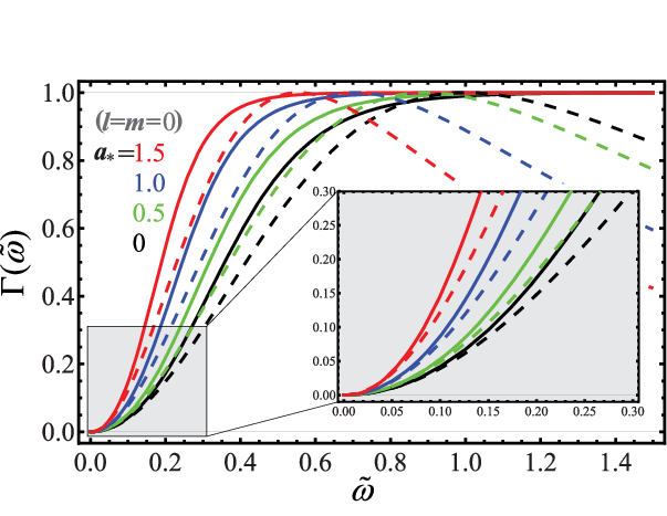
where (28) is also used. Straightforward computation of the gamma function in Eq. (30) leads exactly to the same equation in Ida:2002ez⁴⁴ 4 In the Ref. Ida:2002ez, the greybody factor was written in terms of $C\equiv-i(C_{1}/C_{2})$.. In Fig. 1, the exact solutions and approximate solutions in the low frequency limit are compared for the simplest mode, $(l,m)=(0,0)$. The rotation parameter $a_{*}$ varies from zero to the maximum possible value $a_{*{\rm max}}=1.5$.

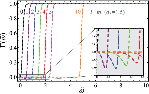
In Fig. 2, the greybody factor curves of the exact solutions are also compared to the numerical results Ida:2005ax. We plot these two results for the various $l=m$ modes with the rotation parameter, $a_{*}=a_{*{\rm max}}$, whose graphs show overlaps.

In low scale gravity scenarios, higher dimensional rotating black holes are copiously produced in high energy collisions, which may be within the reach of the high energy LHC or future circular collider at CERN or China with $\sqrt{s}=100$ TeV. The detection of Hawking radiation from a higher dimensional rotating black hole may be the most interesting way of proving not only the large or warped extra dimensions ⁵⁵ 5 In Orlando:2010kx, black holes from the compact hyperbolic extra dimensions are discussed, but also the quantum phenomenon of gravity Cardoso:2012qm.

To support the experimental searches of such signal and theoretical interest by its own, there have been significant theoretical studies on the Hawking radiation for higher dimensional rotating black holes in both the analytical and numerical ways. Before this paper, the analytic studies have been successful only in the specific regimes, e.g., low-frequency regime or high-frequency regime. In the present work, we are successful in finding the full solution of the generalized Teukolsky equation without assuming any limitation in the frequency domain for the brane scalar modes in 5D black hole background of Myers-Perry solution.

The obtained exact result enables us to describe the Hawking radiation in the entire frequency regime and to analyze its characters in detail. Since the detailed study of greybody factors allow us to have a better understanding of quantum nature of black holes, the study with various approaches will give us some insight into the fundamental properties of black holes. Therefore the exact form of the greybody factor of scalar perturbations for the 5D black holes may provide a good approach for the extra dimension search and development of quantum gravity.

Finally, we comment on the Teukolsky equation for the higher spin fields with $s=1/2,1,2/3$, and $2$. We have shown that those high spin states are governed by the confluent Heun equation with complex parameters, which still lack of understanding its basic mathematical properties, yet. Intriguingly, the equation has the same mathematical structure with that of the four-dimensional Kerr black hole Mano:1996vt; Mano:1996gn; Sasaki:2003xr. Thus, finding analytic solutions in one side would provide the greybody factor on the other side, which is definitely worth more attention for the future.

References

- (1) N. Arkani-Hamed, S. Dimopoulos and G. R. Dvali, Phys. Lett. B 429, 263 (1998) [hep-ph/9803315].
- (2) I. Antoniadis, N. Arkani-Hamed, S. Dimopoulos and G. R. Dvali, Phys. Lett. B 436, 257 (1998) [hep-ph/9804398].
- (3) N. Arkani-Hamed, S. Dimopoulos and G. R. Dvali, Phys. Rev. D 59, 086004 (1999) [hep-ph/9807344].
- (4) L. Randall and R. Sundrum, Phys. Rev. Lett. 83, 3370 (1999) [hep-ph/9905221].
- (5) L. Randall and R. Sundrum, Phys. Rev. Lett. 83, 4690 (1999) [hep-th/9906064].
- (6) S. Dimopoulos and G. L. Landsberg, Phys. Rev. Lett. 87, 161602 (2001) doi:10.1103/PhysRevLett.87.161602 [hep-ph/0106295].
- (7) S. B. Giddings and S. D. Thomas, Phys. Rev. D 65, 056010 (2002) doi:10.1103/PhysRevD.65.056010 [hep-ph/0106219].
- (8) L. A. Anchordoqui, J. L. Feng, H. Goldberg and A. D. Shapere, Phys. Rev. D 65, 124027 (2002) doi:10.1103/PhysRevD.65.124027 [hep-ph/0112247].
- (9) J. L. Feng and A. D. Shapere, Phys. Rev. Lett. 88, 021303 (2002) doi:10.1103/PhysRevLett.88.021303 [hep-ph/0109106].
- (10) A. Ringwald and H. Tu, Phys. Lett. B 525, 135 (2002) doi:10.1016/S0370-2693(01)01421-6 [hep-ph/0111042].
- (11) Y. Jho and S. C. Park, arXiv:1806.03063 [hep-ph].
- (12) M. Cavaglia, Int. J. Mod. Phys. A 18, 1843 (2003) doi:10.1142/S0217751X03013569 [hep-ph/0210296].
- (13) P. Kanti, Int. J. Mod. Phys. A 19, 4899 (2004) doi:10.1142/S0217751X04018324 [hep-ph/0402168].
- (14) S. C. Park, Prog. Part. Nucl. Phys. 67, 617 (2012) doi:10.1016/j.ppnp.2012.03.004 [arXiv:1203.4683 [hep-ph]].
- (15) S. W. Hawking, Commun. Math. Phys. 43, 199 (1975) [Commun. Math. Phys. 46, 206 (1976)].
- (16) R. Emparan, G. T. Horowitz and R. C. Myers, Phys. Rev. Lett. 85, 499 (2000) doi:10.1103/PhysRevLett.85.499 [hep-th/0003118].
- (17) S. A. Teukolsky, Phys. Rev. Lett. 29, 1114 (1972).
- (18) D. Ida, K. -y. Oda and S. C. Park, Phys. Rev. D 67, 064025 (2003) [Erratum-ibid. D 69, 049901 (2004)] [hep-th/0212108].
- (19) D. Ida, K. -y. Oda and S. C. Park, Phys. Rev. D 71, 124039 (2005) [hep-th/0503052].
- (20) D. Ida, K. -y. Oda and S. C. Park, Phys. Rev. D 73, 124022 (2006) [hep-th/0602188].
- (21) S. Creek, O. Efthimiou, P. Kanti and K. Tamvakis, Phys. Rev. D 75, 084043 (2007) [hep-th/0701288].
- (22) S. Creek, O. Efthimiou, P. Kanti and K. Tamvakis, Phys. Rev. D 76, 104013 (2007) [arXiv:0707.1768 [hep-th]].
- (23) R. Jorge, E. S. de Oliveira and J. V. Rocha, Class. Quant. Grav. 32, no. 6, 065008 (2015) [arXiv:1410.4590 [gr-qc]].
- (24) C. M. Harris and P. Kanti, Phys. Lett. B 633, 106 (2006) doi:10.1016/j.physletb.2005.10.025 [hep-th/0503010].
- (25) G. Duffy, C. Harris, P. Kanti and E. Winstanley, JHEP 0509, 049 (2005) doi:10.1088/1126-6708/2005/09/049 [hep-th/0507274].
- (26) M. Casals, P. Kanti and E. Winstanley, JHEP 0602, 051 (2006) doi:10.1088/1126-6708/2006/02/051 [hep-th/0511163].
- (27) M. Casals, S. R. Dolan, P. Kanti and E. Winstanley, JHEP 0703, 019 (2007) doi:10.1088/1126-6708/2007/03/019 [hep-th/0608193].
- (28) T. Harmark, J. Natario and R. Schiappa, Adv. Theor. Math. Phys. 14, no. 3, 727 (2010) doi:10.4310/ATMP.2010.v14.n3.a1 [arXiv:0708.0017 [hep-th]].
- (29) R. C. Myers and M. J. Perry, Annals Phys. 172, 304 (1986).
- (30) V. P. Frolov and D. Stojkovic, “Quantum radiation from a five-dimensional rotating black hole,” Phys. Rev. D 67, 084004 (2003) [gr-qc/0211055].
- (31) A. Ronveaux, Heun’s Differential Equations (Oxford University Press, Oxford Oxfordshire, 1995).
- (32) Meixner J. and Schäfke F. W., Mathieusche Funktionen und Sphäroidfunktionen (Berlin: Springer, 1954).
- (33) J. Meixner, F. W. Schäfke, and G. Wolf, Mathieu Functions and Spheroidal Functions and Their Mathematical Foundations (Further Studies) (Lecture Notes in Mathematics, vol 837) (Berlin: Springer, 1980).
- (34) P. E. Falloon, P. C. Abbott, and J. B. Wang, J. Phys. A 36:5477–5495 (2003).
- (35) V. Cardoso et al., Class. Quant. Grav. 29, 244001 (2012) doi:10.1088/0264-9381/29/24/244001 [arXiv:1201.5118 [hep-th]].
- (36) D. Orlando and S. C. Park, JHEP 1008, 006 (2010) doi:10.1007/JHEP08(2010)006 [arXiv:1006.1901 [hep-th]].
- (37) D. N. Page, Phys. Rev. D 13, 198 (1976).
- (38) S. Mano, H. Suzuki and E. Takasugi, Prog. Theor. Phys. 95, 1079 (1996) [gr-qc/9603020].
- (39) S. Mano and E. Takasugi, Prog. Theor. Phys. 97, 213 (1997) [gr-qc/9611014].
- (40) M. Sasaki and H. Tagoshi, Living Rev. Rel. 6, 6 (2003) [gr-qc/0306120].