Learning for Multi-Model and Multi-Type Fitting
Abstract
Multi-model fitting has been extensively studied from the random sampling and clustering perspectives. Most assume that only a single type/class of model is present and their generalizations to fitting multiple types of models/structures simultaneously are non-trivial. The inherent challenges include choice of types and numbers of models, sampling imbalance and parameter tuning, all of which render conventional approaches ineffective. In this work, we formulate the multi-model multi-type fitting problem as one of learning deep feature embedding that is clustering-friendly. In other words, points of the same clusters are embedded closer together through the network. For inference, we apply K-means to cluster the data in the embedded feature space and model selection is enabled by analyzing the K-means residuals. Experiments are carried out on both synthetic and real world multi-type fitting datasets, producing state-of-the-art results. Comparisons are also made on single-type multi-model fitting tasks with promising results as well.
1 Introduction
Multi-model fitting has been a key problem in computer vision for decades. It aims to discover multiple independent structures, e.g. lines, circles, rigid motions, etc, often in the presence of noise. Here, by multi-model, we mean there are multiple models of a specific type, e.g. lines only. If in addition, there is a mixture of types (e.g. both lines and circles), we specifically term the problem as multi-model multi-type.
Various attempts towards solving the multi-model clustering problem have been made. The early works tend to be based on extensions of RANSAC fischler1981random to the multi-model setting, e.g. simply running RANSAC multiple times consecutively torr1998geometric; vincent2001detecting. More recent works in this approach involve analyzing the interplay between data and hypotheses. J-Linkage toldo2008robust, its variant T-Linkage Magri2014 and ORK Chin2009; chin2010accelerated rely on extensively sampling hypothesis models and compute the residual of data to each hypothesis. Either clustering is carried out on the mapping induced by the residuals, or an energy minimization is performed on the point to model distance, and various regularization terms (e.g. the label count penalty li2007two and spatial smoothness (PEaRL) Isack2012). Another class of approach involves direct analytic expressions characterizing the underlying subspaces, e.g., the powerful self-expressiveness assumption has inspired various elegant methods Elhamifar2013; liu2013robust; Li2015; Ji2016.
Despite the considerable development of multi-model fitting techniques in the past two decades, there are still major lacuna in the problem. First of all, in contrast with having multiple instances of the same type/class, many real world model fitting problem consists of data sampled from multiple types of models. Fig. 1 shows both a toy example of line, circle and ellipses co-existing together, and a realistic motion segmentation scenario, where the appropriate model to fit the foreground object motions (or even the background) can waver between affine motions, homography, and fundamental matrix xu2018motion with no clear division. With few exceptions Barath2018; sugaya2004geometric; torr1998geometric, none of the aforementioned works have considered this realistic scenario. Even if one attempts to fit multiple types of model sequentially like in sugaya2004geometric, it is non-trivial to decide the type when the dichotomy of the models is unclear in the first place. Secondly, for problems where there are a significant number of models, the hypothesis-and-test approach is often overwhelmed by sampling imbalance, i.e., points from the same subspace represent only a minority, rendering the probability of hitting upon the correct hypothesis very small. This problem becomes severe when a large number of data samples are required for hypothesizing a model (e.g., eight points are needed for a linear estimation of the fundamental matrix and 5 points for fitting an ellipse). Lastly, for optimal performance, there is inevitably a lot of manipulation of parameters needed, among which the most sensitive include those for deciding what constitutes an inlier for a model Magri2014; Magri2015, for sparsifying the affinity matrices Lai2017; xu2018motion, and for selecting the model type torr1998geometric. Often, dataset-specific tuning is required, with very little theory to guide the tuning.

There has been some recent foray into deep learning as a means to learn geometric model, e.g. camera pose brachmann2017dsac and essential matrix yi2018learning from feature correspondences, but extending such deep geometric model fitting approach to the multi-model and multi-type scenario has not been attempted. Generalizing the deep learning counterparts of RANSAC to multi-model fitting is not trivial due to the same reason as conventional sequential approaches. Furthermore, in many geometric model fitting problems, there are often significant overlap between the subspaces occupied by the multiple model instances (e.g. in motion segmentation, both the foreground and the background contain the camera-induced motion). We want the network to learn the best representation so that the different model instances can be well-separated. This is in contrast to the traditional clustering approaches where hand-crafted design of the similarity metric is needed.When there are no clear division between multiple types of models (e.g. the transitions from a circle to an ellipse), the network would also need to learn the appropriate preference from the labelled examples in the training data.
Another open challenge in multi-model fitting is to automatically determine the number of models, also referred to as model selection in the literature Tibshirani2001; Chin2009; Li_2013_ICCV; Lai2017. Traditional methods proceed from statistical analysis of the residual of the clustering Tibshirani2001; rousseeuw1987silhouettes. Other methods approach from various heuristic standpoints including analyzing eigen values zelnik2005self; von2007tutorial, over-segment and merge Li_2013_ICCV; Lai2017, soft thresholding liu2013robust or adding penalty terms Li2014. Most of the above works cannot deal with mixed-types in the models. To redress this gap in the literature, we want our network to learn good feature representations so that the number of clusters, even in the presence of mixed types, can be readily estimated.
With the above objectives in mind, we propose a multi-model multi-type fitting network. The network is given labelled data (inlier points for each model and outliers) and is supposed to learn the various geometric models in a completely data-driven manner. Since the input to the network is often not regular grid data like images, we use what we called the CorresNet from yi2018learning as a backbone (see Fig. 2). As the output of network should be amenable for grouping into the respective, possibly mixed models, and invariant to any permutation of model indices among the multiple instances of the same class in the training data, we consider both an existing metric learning loss and its variant and propose a new distribution aware loss, the latter based on Fisher linear discriminant analysis (LDA). In the testing phase, standard K-means clustering is applied to the feature embeddings to obtain a discrete cluster assignment. As feature points are embedded in a clustering friendly way, we can just look into the K-means fitting residual to estimate the number of models should it be unknown.
2 Related Work
Multi-Model Fitting: Early approaches address this in a sequential RANSAC fashion torr1998geometric; vincent2001detecting; Yasushi2004. These algorithms iteratively fit one model per iteration using RANSAC and remove the inliers of the best model. The J-Linkage toldo2008robust and its variant T-Linkage Magri2014 simultaneously consider the interactions between all points and hypotheses. The final partition is achieved in an agglomerative clustering manner. The above greedy algorithms often do not perform well under high noise level. In contrast, global algorithms have been proposed to minimize an energy with various regularization terms. These include spatial regularization (PEaRL) Isack2012 and label count penalty li2007two. An EM-like algorithm is often adopted to iteratively minimize the energy until convergence. Other works that are based on such hypothesis-and-test paradigm adopt spectral clustering in the final grouping step Chin2009; chin2010accelerated. In contrast to the iterative approaches, analytic approaches are characterized by elegant mathematical formulation, the most well-known among them being those based on the sparsity Elhamifar2013 and low-rank liu2013robust assumptions and their variants. Nonetheless, very few works Barath2018; goh2007segmenting; sugaya2004geometric; torr1998geometric have considered the problem of fitting multiple model of various types, and in these few works, the types are assumed to be known a priori, well-defined, and cleanly separable, which is often not the case.
Deep Learning for Geometric Problems: Using deep learning to solve geometric model fitting has received growing considerations. The dense approaches start from raw image pairs to estimate models such as homography detone2016deep or non-rigid transformation rocco2017convolutional. melekhov2017relative proposed to estimate the camera pose directly from image sequences.
In contrast to the preceding works, DSACbrachmann2017dsac learns to extract from sparse feature correspondences some geometric models in a manner akin to RANSAC. The ability to learn representations from sparse points was also developed recentlyQi2017; QiLSG_NIPS2017. This ability was exploited by yi2018learning to fit camera motion (essential matrix) from noisy correspondences. Despite the promising results, none of the existing works have considered generic model fitting and, more importantly, fitting data of multiple models and even multiple types. In this work, we formulate the generic multi-model multi-type fitting problem as one of learning good representations for clustering.
Deep Learning for Clustering: One line of researches tackle the problem by minimizing the reconstruction loss huang2007unsupervised; vincent2008extracting; lee2009convolutional. The reconstruction loss can be further combined with various losses for achieving clustering objectives tian2014learning; yang2016joint; ji2017deep; xie2016unsupervised. Among these, the k-means loss was proposed by yang2016joint optimizing the points to cetner distance. xie2016unsupervised proposed to minimize the KL-Divergence between the original feature and the embedded features. The locality-preserving loss huang2014deep aims to find feature embedding conforming to a manifold constraint.These works learn feature embedding in an unsupervised fashion. When faced with the greater ambiguity envisaged in our multi-type fitting tasks, these unsupervised approaches are likely to face difficulties. For example, feature points on near planar foreground and background with large depth variation cannot be easily separated without proper assumption.
To take advantage of labelled data, metric learning has been applied to clustering Xing2003; hershey2016deep. With the advent of deep neural network, works in metric learning tend to focus on designing metric learning lossesChopra2005; Schroff2015; Sohn2016; hershey2016deep; song2017deep. Among these, hershey2016deep minimizes the L2 distance between the predicted and ground-truth affinities and provides a competitive baseline. To further take the global points distribution, we propose the clustering-specific loss MaxInterMinIntra, which optimize the inter-cluster separation and intra-cluster variance.
3 Methodology
In this section, we first explain the training process of our multi-model multi-type fitting network. We then introduce existing metric learning loss and our MaxInterMinIntra loss.
3.1 Network Architecture
We denote the input sparse data with points as where each individual point is . The input sparse data could be geometric shapes, feature correspondences in two frames or feature trajectories in multiple frames. We further denote the one-hot key encoded labels accompanying the input data as where and is the number of clusters or partitions of the input data.
Cascaded multi-layer perceptrons (mlps) has been used to learn feature representation from generic point input Qi2017; yi2018learning. We adopt a backbone network similar to CorresNet yi2018learning11 1 Alternative sparse data networks, e.g. PointNet Qi2017, are applicable as well shown in Fig. 2 . The output embedding of the CorresNet is denoted as . To make the output clustering-friendly, we apply a differentiable, clustering-specific loss function , measuring the match of the output feature representation with the ground-truth labels. The problem now becomes that of learning a CorresNet backbone that minimizes the loss .
3.2 Clustering Loss
We expect our clustering loss function to have the following characteristics. First, It should be invariant to permutation of models, e.g. the order of these models are exchangeable. Second the loss must be adaptable to varying number of groups. Lastly, the loss should enable good separation of data points into clusters. We consider the following loss functions.
L2Regression Loss: Given the ground-truth labels and the output embeddings , the ideal and reconstructed affinity matrices are respectively,
| (1) |
The training objective is to minimize the difference between and measured by element-wise L2 distance hershey2016deep.
| (2) |
The above L2 Regression loss is obviously differentiable w.r.t. . Since the output embedding is L2 normalized, the inner product between two point representations is .
Cross-Entropy Loss: As alternative to the L2 distance, one could measure the discrepancy between and as KL-Divergence. Since , where is the entropy function and is the sigmoid function, with fixed , we simply need to minimize the cross-entropy which derives the following element-wise cross-entropy loss,
| (3) |
The cross-entropy loss is more likely to push points and of the same cluster together faster than L2Regression, i.e. inner product and those of different clusters apart, i.e. inner product .
MaxInterMinIntra Loss: Both the above losses consider the pairwise relation between points; the overall point distribution in the output embedding is not explicitly considered. We now propose a new loss which takes a more global view of the point distribution rather than just the pairwise relations. Specifically, we are inspired by the classical Fisher LDA fisher1936use. LDA discovers a linear mapping that maximizes the distance between class centers/means and minimizes the scatter/variance within each class . Formally, the objective for a two-class problem is written as,
| (4) |
which is to be maximized over . For linearly non-separable problem, one has to design kernel function to map the input features before applying the LDA objective. Equipped now with more powerful nonlinear mapping networks, we adapt the LDA objective—for the multi-class scenarios—to perform these mappings automatically as below,
| (5) |
where , and indicating the set of points belonging to cluster . We use the extremas of the inter-cluster distances and intra-cluster scatters (see Fig. 3) so that the worst case is explicitly optimized. Hence, we term the loss as MaxInterMinIntra (MIMI). By applying log operation on the objective,we arrive at the following loss function to be minimized:

| (6) |
One can easily verify that the MaxInterMinIntra loss is differentiable w.r.t. . We give the gradient in Eq (7).
Optimization: The Adam optimizer kingma2014adam is used to minimize the loss . The learning rate is fixed at and mini-batch at one frame pair or sequence. The mini-batch size cannot exceed one because the number of points/correspondences is not uniform across different sequences. For all tasks, we train the network 300 epochs.
|
|
(7) |
3.3 Inference
During testing, we apply standard K-means to the output embeddings . This step is applicable to both multi-model and multi-type fitting problems, as we do not need to specify explicitly the type of model to fit. Finally, with unknown number of models , we propose to analyze the K-means residuals,
| (8) |
Good estimate of often yields low and further increasing does not significantly reduce . So we find the at the ‘elbow’ position. We adopt two off-the-shell approaches for this purpose, the second order difference (SOD)Zhang2012 and silhouette analysis rousseeuw1987silhouettes. Both are parameter-free.
4 Experiment
We demonstrate the performance of our network on both synthetic and real world data, with extensive comparisons with traditional geometric model fitting algorithms. Our focus is on the multi-type setting (the first two experiments on LCE and KT3DMoSeg), but we also carry out experiments on the pure multi-model scenario (LCE-unmixed and Adelaide RMF) experiments.
4.1 Datasets
Synthesized Lines, Circles and Ellipses (LCE): Fitting ellipses has been a fundamental problem in computer vision fitzgibbon1999direct. We synthesize for each sample four different types of conic curves in a 2D space, specifically, one straight line, two ellipses and one circle. We randomly generate 8,000 training samples, 200 validation samples and 200 testing samples. Each point is perturbed by adding a gaussian noise with .
KT3DMoSeg xu2018motion: This benchmark was created based upon the KITTI self-driving datasetGeiger2013IJRR with 22 sequences in total. Each sequence contains two to five rigid motions. As analyzed by xu2018motion, the geometric model for each individual motion can range from an affine transformation, a homography, to a fundamental matrix, with no clear dividing line between them. We evaluate this benchmark to demonstrate our network’s ability to tackle multi-model multi-type fitting. For fair comparison with all existing approaches, we only crop the first 5 frames of each sequence for evaluation, so that the broken trajectory does not give undue advantage to certain methods.
Synthesized Lines, Circles and Ellipses Unmixed (LCE-Unmixed): To demonstrate the ability of our network on single-type multi-model fitting, we also randomly generate in each sample a single class of conic curves in 2D space (lines, circles, or ellipses) but with multiple instances (2-4) of them. The number of training, validation and testing samples are the same as those of the multi-type LCE setting. Same perturbation as LCE is applied here.
Adelaide RMF Dataset wong2011dynamic: This dataset consists of 38 frame pairs, of which half are designed for multi-model fitting (the model being homographies induced by planes). The number of planes is between two to seven. The other 19 frame pairs are designed for two-view motion segmentation. It is nominally a single-type multiple fundamental matrix fitting problem and has been treated as such by the community. While we put the results under the single-type category, we hasten to add that there might indeed be degeneracies, i.e. near planar rigid objects, (and hence mixed types) present in this dataset, no matter how minor. The number of motions is between one to five.
4.2 Multi-Type Curve Fitting
The multiple types in this curve fitting task comprises of lines, circles, and ellipses in the LCE dataset. Note that there is no clear dividing boundary between them as they can be all explained by the general conic equation (with the special cases of lines and circles obtained by setting some coefficients to ):
| (9) |
There are two ways to adapt the traditional multi-model methods for this multi-type setting. One approach is to formulate the multi-type fitting problem as fitting multiple models parameterized by the same conic equation in Eq (9). This approach is termed HighOrder (H.O.) fitting. Alternatively, one could sequentially fit three types of models, which is termed Sequential (Seq.) fitting. For ellipse-specific fitting, the direct least square approach fitzgibbon1999direct is adopted. For our model, we evaluate the various metric learning losses introduced in Section 3.2 and present the results in Tab. 1. The results are reported with the optimal setting determined by the validation set. We evaluate the performance by two clustering metrics, Classification Error Rate (Error Rate), i.e. the best classification results subject to permutation of clustering labels, and Normalize Mutual Information (NMI). Comparisons are made with state-of-the-art multi-model fitting algorithms including T-linkage Magri2014, RPA Magri2015 and RansaCov magri2016multiple. We notice that T-linkage returns extremely over-segmented results in the sequential setting, e.g. more than 10 lines, making classification error evaluation intractable as it involves finding the permutation label with lowest error rate. For our model, we evaluate the three loss variants, the L2 Regression loss (L2), Cross Entropy loss (CE) and MaxInterMinIntra loss (MIMI).
| Mdl. | T-LinkageMagri2014 | RPAMagri2015 | RansaCovmagri2016multiple | Our Models | |||||
| H.O. | Seq. | H.O. | Seq. | H.O. | Seq. | L2 | CE | MIMI | |
| Err | 52.14 | - | 39.43 | 23.17 | 40.57 | 24.04 | 18.49 | 18.32 | 18.04 |
| NMI | 0.340 | - | 0.464 | 0.667 | 0.394 | 0.604 | 0.713 | 0.720 | 0.727 |
We make the following observations about the results. First, all our metric learning variants outperform the HighOrder and Sequential multi-type fitting approaches. Second, the all-encompassing model used in the HighOrder approach suffers from ill-conditioning when fitting simpler models. Thus, the performance is much inferior to that of Sequential fitting. However, it is worth noting that despite the Sequential approach being given the strong a priori knowledge of both the model type and the number of model for each type, its performance is still significantly worse off than ours.
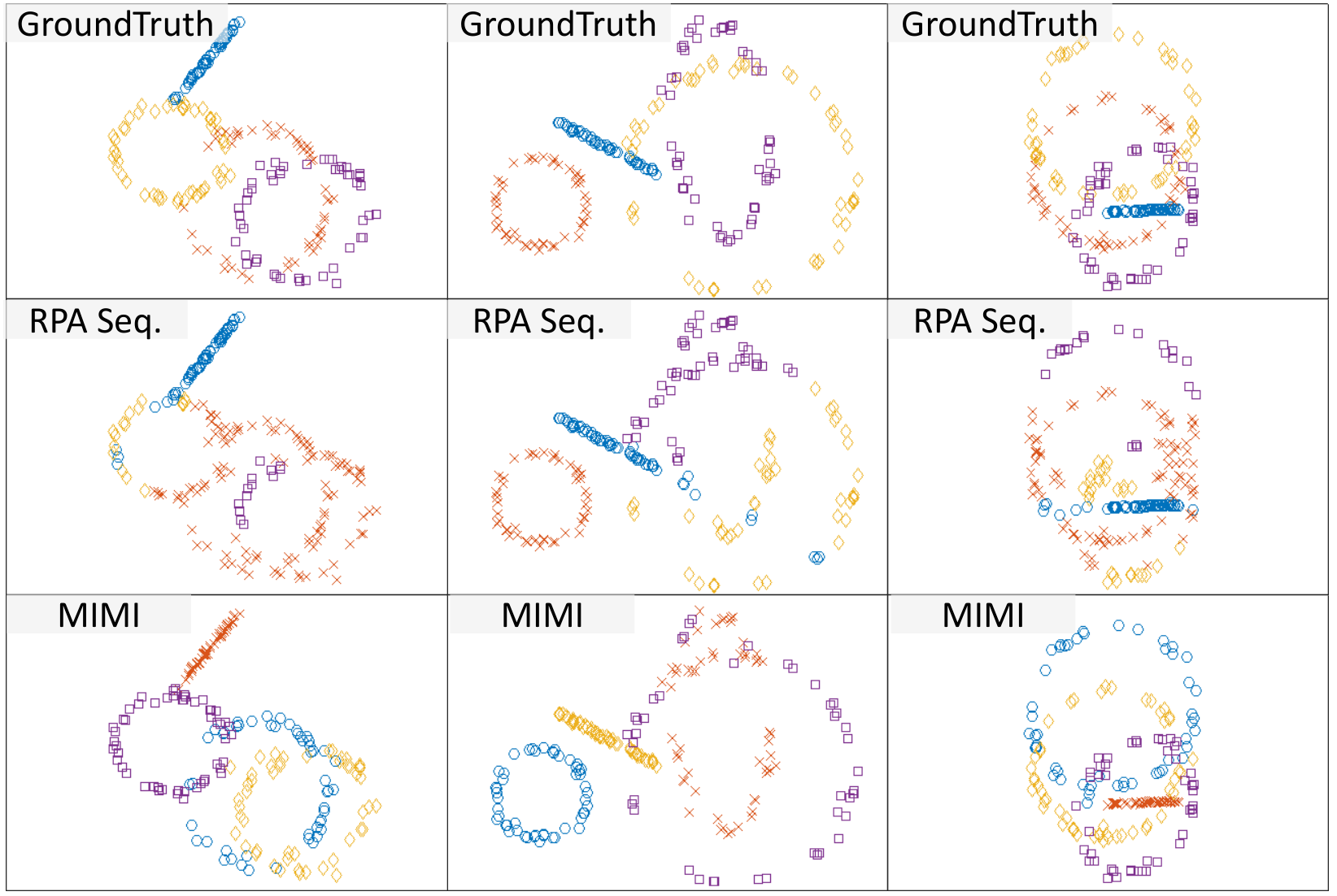
For qualitative comparison, we visualize the ground-truth and segmentation results of each method in Fig. 4. Our clustering results on the bottom row show success in discovering all individual shapes with mistakes made only at the intersections of individual structures. Though good at separating straight line, the RPA failed to discover ellipses as sampling all 5 inliers amidst the large number of outliers and fitting an ellipse from even correct 5 support points with noise (noise in coordinate) are both very difficult, the latter demonstrated in fitzgibbon1999direct.
4.3 Multi-Type Motion Segmentation
The KT3DMoSeg benchmark xu2018motion is put forth for the task of motion segmentation. Each sequence often consists of a background whose motion can be explained in general by a fundamental matrix while the models for the foreground motions can sometimes be ambiguous due to the limited spatial extent of the objects, thus giving rise to mixed types of models. For example, in Fig. 5, the vehicles in ‘Seq009_Clip01’ and ‘Seq028_Clip03’ can be roughly explained by an Affine transformation or Homography while the oil tanker in ‘Seq095_Cip01’ should be modeled by a fundamental matrix. Even the background motion can be ambiguous to model, when the background is dominated by a plane, for instance, the quasi-planar row of trees on the right side of the road in ‘Seq028_Clip03’ is likely to lead to degeneracies in the fundamental matrix estimation and thus cause errors in the traditional method (second row). For this dataset, we use the first five frames of each sequence for fair comparison and apply leave-one-out cross-validation, i.e. repeatedly train on 21 sequences and test on the left-out sequence; we dubbed this the ‘Vanilla’ setting. Each sequence has between 10-20 frames, so we could further increase the training data by augmenting with all the remaining five-frame clips from each sequence with no overlap; this is termed as the ‘Augment’ setting. The testing clips (first five frames of each sequence) are kept the same for both settings. We compare with subspace clusering approaches, GPCAvidal2005generalized, LSAYan2006, ALCRao2010, LRRliu2013robust, MSMCDragon2012 and SSCElhamifar2013 and the multi-view clustering (MVC) methods in xu2018motion. Results are presented in Tab. 2.
| Model | State-of-the-Arts | Our Models | |||||||||||
| GPCAvidal2005generalized | ALCRao2010 | LSAYan2006 | LRRliu2013robust | MSMCDragon2012 | SSCElhamifar2013 | MVCxu2018motion | Vanila | Augment | |||||
| L2 | CE | MIMI | L2 | CE | MIMI | ||||||||
| Mean Err | 36.46 | 15.17 | 36.3 | 22.00 | 32.74 | 26.62 | 10.99 | 14.04 | 12.44 | 14.15 | 8.87 | 11.48 | 6.78 |
| Med. Err | 33.93 | 16.42 | 40.3 | 18.16 | 36.48 | 29.14 | 6.57 | 8.90 | 9.87 | 10.89 | 6.68 | 9.42 | 2.67 |
We make the following observations about the results. Our vanilla leave-one-out approach achieved very competitive performance on all 22 sequences in KT3DMoSeg. In the ‘Augment’ setting, our approach even outperforms the state-of-the-art multi-view clustering approaches (MVC) xu2018motion. Of all benchmark methods, only MVC has considered the multi-type fitting issue. However, the multi-view fusion proposed therein still does not guarantee that each rigid motion is explained by the correct model. Furthermore, we notice that our proposed MIMI metric is comparable to both the L2 Regression and cross entropy loss and gives even lower error when augmented with additional data. This suggests that optimizing the distribution of the embedded features with a clustering-specific loss is effective.
Finally, we present qualitative comparison between the results of MVC and ours in Fig. 5. Not only is the proposed network capable of correctly segmenting the aforementioned degenerate motions, it surpasses our expectations in how it performs in ‘Seq009_Clip01’. Here the independently moving car (the yellow group in the ground truth image) has a flow field that is consistent with the epipolar constraint associated with the background motion (due to them both translating in the same direction) xu2018motion. Without resorting to reconstructing the depth of the car, it would be impossible to separate it from the background. However, criteria involving depth would be very unwieldy to specify analytically in the existing approaches. Here, without having any preconceived notion of the geometrical model, our network seems to have learnt the requisite criteria to separate the independent motion.

4.4 Multi-Model Fitting
In this section, we further demonstrate the ability of our network to handle conventional (i.e., single-type) multi-model fitting problems.
Synthetic Multi-Model Fitting: In this experiment, we evaluate multi-model fitting of a single type (the type being line, circle or ellipse). We adopt a similar training and testing split as in the synthetic LCE task, i.e. 8,000 training samples and 200 testing samples and compare with RPAMagri2015. The results are presented in Fig. 6. We conclude from the figure that, first, our multi-model network performs comparably with RPA on multi-line segmentation task while outperforming RPA with large margin on the more challenging multi-circle and multi-ellipse segmentation tasks. Moreover, the performance drops sharply (higher error) from multi-line (blue) to multi-ellipse (green) fitting for RPA, with the drop getting more acute as the number of model increases. This suggests that the increasing size of the minimal support set (2 points for line, 3 points for circle and 5 points for ellipse) introduces great challenge for the Ransac-based approaches due to sampling imbalance. Hitting the true model becomes very difficult for model with larger support set and experiencing higher noise level. It is evident that our multi-model network is less sensitive to the complexity of the model, as the drop in performance (purple and cyan bars) are less significant. Fig. 6 thus demonstrates that our deep learning approach is better able to deal with sampling imbalance, probably by picking up and leveraging on the additional regularity in the way the points are distributed.
Two-View Multi-Model Fitting: Finally, we evaluate the multi-model fitting task on the Adelaide RMF dataset wong2011dynamic. For both the multi-planar and motion segmentation tasks, we carry out a leave-one-out cross-validation. For fair comparison, we report the classification error rate (ErrorRate). The state-of-the-art models being compared include J-Linkage toldo2008robust, T-LinkageMagri2014, RPA Magri2015, RCMSA pham2014random and ILP-RansaCovmagri2016multiple. The comparisons are presented in Tab. 3. We observe that our multi-model network gives very competitive results on both the multi-planar and motion segmentation tasks. For the former task, our proposed MaxInterMinIntra (MIMI) loss yields which is better than many benchmark models. For the motion segmentation task, our model with L2 Regression loss gives a mean error of . We note the performance is achieved by training on only a very small amount of data (18 sequences) and without any dataset-specific parameter tuning. We further note that here, without the problems posed by mixed types, the traditional methods are able to reap the benefits of the given geometrical models (an advantage compared to our method which does not have any preconceived model).
| Model | MultiHomo | MoSeg | |||
| Mean | Med. | Mean | Med. | ||
| State-of-the-arts | J-Linkagetoldo2008robust | 25.50 | 24.48 | 16.43 | 14.29 |
| T-LinkageMagri2014 | 24.66 | 23.38 | 9.36 | 7.80 | |
| RCMSApham2014random | 28.30 | 29.40 | 12.37 | 9.87 | |
| RPAMagri2015 | 17.20 | 17.53 | 5.49 | 4.57 | |
| ILP-RansaCovmagri2016multiple | 12.91 | 12.34 | 6.04 | 4.27 | |
| Ours | Loss | ||||
| L2Regress | 17.55 | 14.77 | 8.98 | 7.50 | |
| CrossEnt | 17.88 | 12.10 | 9.07 | 5.79 | |
| MIMI | 17.33 | 12.00 | 9.39 | 6.50 | |
4.5 Further Study
In this section, we first further analyze the impact of metric learning on transforming the point feature representations. Then we present results on model selection and finally do ablation study for the proposed MaxInterMinIntra loss.
Feature Embedding To gain some insight on how the learned feature representations are more clustering-friendly, we provide direct visualization of the representations. For that purpose, we use T-SNEmaaten2008visualizing to project both the KT3DMoSeg raw feature points (of dimension ten for 5 frames) and network output embeddings to a 2-dimensional space. Three example sequences are presented in the last row of Fig. 5. We conclude from the figure that: (i) the original feature points are hard to be grouped by K-means correctly; and (ii) after our network embedding, feature points are more likely to be grouped according to the respective motions, regardless of the underlying types of motions.
Model Selection: As can be seen from Fig. 5, the point distribution in the learned feature embedding is amenable for model selection (estimating the number of clusters/motions). We evaluate both Second Order Difference (SOD)liu2013robust and Silhouette Analysis (Silh.) rousseeuw1987silhouettes to estimate the number of motions. We also compare with alternative subspace clustering approaches with built-in model selection, namely, LRR liu2013robust and MSMC Dragon2012 and additionally apply self-tuning spectral clustering(S.T.) zelnik2005self to the affinity matrix obtained in MVC xu2018motion. Performances are evaluated in terms of mean classification error (Err.) and correct rate (Corr.), i.e. the percentage of samples/sequences with correctly estimated number of cluster (higher the better). Comparisons are presented in Tab. 4. Thanks to the deep feature learning, both SOD and Silh. applied to our method give strong performance even though they are very simple heuristics.
| Method | MIMI Loss | S.T.zelnik2005self | LRRliu2013robust | MSMCDragon2012 | |
| SODliu2013robust | Silh.rousseeuw1987silhouettes | ||||
| Mean Err | 7.36 | 7.25 | 18.16 | 25.08 | 48.29 |
| Correct | 86.36 | 81.82 | 40.91 | 54.55 | 22.73 |
Dimension of Output Embedding: We investigate the impact of the dimension of the output embedding on the performance of multi-model/type fitting. Here, we vary the size of the embedding dimension from 3 to 7 for all three tasks and present the resulting error rates against the dimension in Fig 7 (left). As we can see, the errors are relatively stable w.r.t. the output embed dimension from 4 to 7 for all three tasks with optimal between 5 to 6 coninciding with the maximal number of clusters for each task (max 5 motions for KT3DMoSeg and max 4 structures for Synthetic). Thus the maximal number of clusters serves as a good heuristic for the dimension of the network output embedding.
MIMI Loss: Here we investigate the necessity of both maximizing inter cluster distance and minimizing intra cluster variance. In specific, we compare the following variants. (i) MaxInter: only maximizing the inter cluster distance is considered, equivalent to the first term in Eq (6). (ii) MinIntra: only minimizing the intra cluster variance is considered, the second term in Eq (6). (iii) K-means loss: we further note the k-means loss yang2017towards proposed for unsupervised deep clustering shares the same objective with MinIntra. We therefore adapt the k-means loss to supervised learning with fixed point-to-cluster assignment during training. We compare the three variants with our final MIMI loss on KT3DMoSeg and present the results in Fig. 7 (right). The MIMI loss is consistently better (lower error) than all three variants. In particular, the MinIntra and K-means loss produce large errors. This indicates that pushing points of different clusters away is vital to feature embedding for clustering.
5 Conclusion
In this work, we investigate training a deep neural network for general multi-model and multi-type fitting. We formulate the problem as learning non-linear feature embeddings that maximize the distance between points of different clusters and minimize the variance within clusters. For inference, the output features are fed into a K-means to obtain the grouping. Model selection is easily achieved by just analyzing the K-means residual in a parameter free manner. Experiments are carried out on both synthetic and real geometric multi-model multi-type fitting tasks. Comparison with state-of-the-art approaches proves that our network can better deal with multiple types of models simultaneously, without any preconceived notion of the underlying model. Our method is also less sensitive to sampling imbalance brought about by the increasing number of models, and it works well in a broad range of parameter values, without the kind of careful tuning required in conventional approaches.
References
- (1) D. Barath and J. Matas. Multi-class model fitting by energy minimization and mode-seeking. In CVPR, 2018.
- (2) E. Brachmann, A. Krull, S. Nowozin, J. Shotton, F. Michel, S. Gumhold, and C. Rother. Dsac-differentiable ransac for camera localization. In CVPR, 2017.
- (3) T. Chin, H. Wang, and D. Suter. The ordered residual kernel for robust motion subspace clustering. In NIPS, 2009.
- (4) T.-J. Chin, J. Yu, and D. Suter. Accelerated hypothesis generation for multi-structure robust fitting. In ECCV, 2010.
- (5) S. Chopra, R. Hadsell, and L. Y. Learning a similiarty metric discriminatively, with application to face verification. In CVPR, 2005.
- (6) D. DeTone, T. Malisiewicz, and A. Rabinovich. Deep image homography estimation. arXiv preprint arXiv:1606.03798, 2016.
- (7) R. Dragon, B. Rosenhahn, and J. Ostermann. Multi-scale clustering of frame-to-frame correspondences for motion segmentation. In ECCV, 2012.
- (8) E. Elhamifar and R. Vidal. Sparse subspace clustering: Algorithm, theory, and applications. IEEE Transactions on Pattern Analysis and Machine Intelligence, 2013.
- (9) M. A. Fischler and R. C. Bolles. Random sample consensus: a paradigm for model fitting with applications to image analysis and automated cartography. Communications of the ACM, 1981.
- (10) R. A. Fisher. The use of multiple measurements in taxonomic problems. Annals of eugenics, 7(2):179–188, 1936.
- (11) A. Fitzgibbon, M. Pilu, and R. B. Fisher. Direct least square fitting of ellipses. IEEE Transactions on pattern analysis and machine intelligence, 21(5):476–480, 1999.
- (12) A. Geiger, P. Lenz, C. Stiller, and R. Urtasun. Vision meets robotics: The kitti dataset. International Journal of Robotics Research, 2013.
- (13) A. Goh and R. Vidal. Segmenting motions of different types by unsupervised manifold clustering. In CVPR, 2007.
- (14) J. R. Hershey, Z. Chen, J. Le Roux, and S. Watanabe. Deep clustering: Discriminative embeddings for segmentation and separation. In ICASSP, 2016.
- (15) F. J. Huang, Y.-L. Boureau, Y. LeCun, et al. Unsupervised learning of invariant feature hierarchies with applications to object recognition. In CVPR, 2007.
- (16) P. Huang, Y. Huang, W. Wang, and L. Wang. Deep embedding network for clustering. In ICPR, 2014.
- (17) H. Isack and Y. Boykov. Energy-based geometric multi-model fitting. International Journal of Computer Vision, 2012.
- (18) P. Ji, M. Salzmann, and H. Li. Shape interaction matrix revisited and robustified: Efficient subspace clustering with corrupted and incomplete data. In ICCV, 2016.
- (19) P. Ji, T. Zhang, H. Li, M. Salzmann, and I. Reid. Deep subspace clustering networks. In NIPS, 2017.
- (20) Y. Kanazawa and H. Kawakami. Detection of planar regions with uncalibrated stereo using distributions of feature points. In BMVC, 2004.
- (21) D. P. Kingma and J. Ba. Adam: A method for stochastic optimization. In ICLR, 2015.
- (22) T. Lai, H. Wang, Y. Yan, T. J. Chin, and W. L. Zhao. Motion Segmentation Via a Sparsity Constraint. IEEE Transactions on Intelligent Transportation Systems, 2017.
- (23) H. Lee, R. Grosse, R. Ranganath, and A. Y. Ng. Convolutional deep belief networks for scalable unsupervised learning of hierarchical representations. In ICML, 2009.
- (24) C. G. Li and R. Vidal. Structured Sparse Subspace Clustering: A unified optimization framework. In CVPR, 2015.
- (25) H. Li. Two-view motion segmentation from linear programming relaxation. In CVPR, 2007.
- (26) Z. Li, L. F. Cheong, and S. Z. Zhou. SCAMS: Simultaneous clustering and model selection. In CVPR, 2014.
- (27) Z. Li, J. Guo, L.-F. Cheong, and S. Zhiying Zhou. Perspective motion segmentation via collaborative clustering. In ICCV, 2013.
- (28) G. Liu, Z. Lin, S. Yan, J. Sun, Y. Yu, and Y. Ma. Robust recovery of subspace structures by low-rank representation. IEEE Transactions on Pattern Analysis and Machine Intelligence, 2013.
- (29) L. v. d. Maaten and G. Hinton. Visualizing data using t-sne. Journal of machine learning research, 2008.
- (30) L. Magri and A. Fusiello. T-linkage: A continuous relaxation of J-linkage for multi-model fitting. In CVPR, 2014.
- (31) L. Magri and A. Fusiello. Robust Multiple Model Fitting with Preference Analysis and Low-rank Approximation. In BMVC, 2015.
- (32) L. Magri and A. Fusiello. Multiple model fitting as a set coverage problem. In CVPR, 2016.
- (33) I. Melekhov, J. Ylioinas, J. Kannala, and E. Rahtu. Relative camera pose estimation using convolutional neural networks. In International Conference on Advanced Concepts for Intelligent Vision Systems, 2017.
- (34) T. T. Pham, T.-J. Chin, J. Yu, and D. Suter. The random cluster model for robust geometric fitting. IEEE transactions on pattern analysis and machine intelligence, 2014.
- (35) C. R. Qi, H. Su, K. Mo, and L. J. Guibas. PointNet: Deep learning on point sets for 3D classification and segmentation. In CVPR, 2017.
- (36) C. R. Qi, L. Yi, H. Su, and L. J. Guibas. Pointnet++: Deep hierarchical feature learning on point sets in a metric space. In NIPS, 2017.
- (37) S. Rao, R. Tron, R. Vidal, and Y. Ma. Motion segmentation in the presence of outlying, incomplete, or corrupted trajectories. IEEE Transactions on Pattern Analysis and Machine Intelligence, 2010.
- (38) I. Rocco, R. Arandjelovic, and J. Sivic. Convolutional neural network architecture for geometric matching. In CVPR, 2017.
- (39) P. J. Rousseeuw. Silhouettes: a graphical aid to the interpretation and validation of cluster analysis. Journal of computational and applied mathematics, 1987.
- (40) F. Schroff, D. Kalenichenko, and J. Philbin. FaceNet: A unified embedding for face recognition and clustering. In CVPR, 2015.
- (41) K. Sohn. Improved Deep Metric Learning with Multi-class N-pair Loss Objective. In NIPS, 2016.
- (42) H. O. Song, S. Jegelka, V. Rathod, and K. Murphy. Deep metric learning via facility location. In CVPR, 2017.
- (43) Y. Sugaya and K. Kanatani. Geometric structure of degeneracy for multi-body motion segmentation. In In Workshop on Statistical Methods in Video Processing, 2004.
- (44) F. Tian, B. Gao, Q. Cui, E. Chen, and T.-Y. Liu. Learning deep representations for graph clustering. In AAAI, 2014.
- (45) R. Tibshirani, G. Walther, and T. Hastie. Estimating the number of clusters in a data set via the gap statistic. Journal of the Royal Statistical Society: Series B (Statistical Methodology), 2001.
- (46) R. Toldo and A. Fusiello. Robust multiple structures estimation with j-linkage. In ECCV, 2008.
- (47) P. H. Torr. Geometric motion segmentation and model selection. Philosophical Transactions of the Royal Society of London A: Mathematical, Physical and Engineering Sciences, 1998.
- (48) R. Vidal, Y. Ma, and S. Sastry. Generalized principal component analysis (gpca). IEEE transactions on pattern analysis and machine intelligence, 2005.
- (49) E. Vincent and R. Laganiére. Detecting planar homographies in an image pair. In the 2nd International Symposium on Image and Signal Processing and Analysis, 2001.
- (50) P. Vincent, H. Larochelle, Y. Bengio, and P.-A. Manzagol. Extracting and composing robust features with denoising autoencoders. In ICML, 2008.
- (51) U. Von Luxburg. A tutorial on spectral clustering. Statistics and computing, 2007.
- (52) H. S. Wong, T.-J. Chin, J. Yu, and D. Suter. Dynamic and hierarchical multi-structure geometric model fitting. In ICCV, 2011.
- (53) J. Xie, R. Girshick, and A. Farhadi. Unsupervised deep embedding for clustering analysis. In ICML, 2016.
- (54) E. Xing, M. Jordan, S. Russell, and A. Ng. Distance metric learning with application to clustering with side-information. In NIPS, 2003.
- (55) X. Xu, L. F. Cheong, and Z. Li. Motion segmentation by exploiting complementary geometric models. In CVPR, 2018.
- (56) J. Yan and M. Pollefeys. A General Framework for Motion Segmentation : Degenerate and Non-degenerate. In ECCV, 2006.
- (57) B. Yang, X. Fu, N. D. Sidiropoulos, and M. Hong. Towards k-means-friendly spaces: Simultaneous deep learning and clustering. In ICML, 2017.
- (58) J. Yang, D. Parikh, and D. Batra. Joint unsupervised learning of deep representations and image clusters. In CVPR, 2016.
- (59) K. M. Yi, E. Trulls, Y. Ono, V. Lepetit, M. Salzmann, and P. Fua. Learning to find good correspondences. In CVPR, 2018.
- (60) L. Zelnik-Manor and P. Perona. Self-tuning spectral clustering. In NIPS, 2005.
- (61) T. Zhang, A. Szlam, Y. Wang, and G. Lerman. Hybrid linear modeling via local best-fit flats. International Journal of Computer Vision, 2012.