跳到论文正文
W Papers独立论文阅读器 arXiv:1901.10207 论文正文 计算阅读时间 · 0%
引用这篇论文根据当前论文元数据生成,正式投稿前建议核对。


License: arXiv.org perpetual non-exclusive license
arXiv:1901.10207v2 [nucl-ex] 31 Jan 2019

Measurement of 73Ge(n,γn,\gamma) cross sections and implications for stellar nucleosynthesisJournal: Physics Letters B

C. Lederer-Woods Corresponding author: Corresponding author: claudia.lederer-woods@ed.ac.uk Address: School of Physics and Astronomy, University of Edinburgh, United Kingdom Address: Goethe University Frankfurt, Germany    U. Battino Address: School of Physics and Astronomy, University of Edinburgh, United Kingdom    P. Ferreira Address: Instituto Superior Técnico, Lisbon, Portugal    A. Gawlik Address: University of Lodz, Poland    C. Guerrero Address: Universidad de Sevilla, Spain    F. Gunsing Address: CEA Irfu, Université Paris-Saclay, F-91191 Gif-sur-Yvette, France Address: European Organization for Nuclear Research (CERN), Switzerland    S. Heinitz Address: Paul Scherrer Institut (PSI), Villingen, Switzerland    J. Lerendegui-Marco Address: Universidad de Sevilla, Spain    A. Mengoni Address: Agenzia nazionale per le nuove tecnologie, l’energia e lo sviluppo economico sostenibile (ENEA), Bologna, Italy    R. Reifarth Address: Goethe University Frankfurt, Germany    A. Tattersall Address: School of Physics and Astronomy, University of Edinburgh, United Kingdom    S. Valenta Address: Charles University, Prague, Czech Republic    C. Weiss Address: European Organization for Nuclear Research (CERN), Switzerland Address: Technische Universität Wien, Austria    O. Aberle Address: European Organization for Nuclear Research (CERN), Switzerland    J. Andrzejewski Address: University of Lodz, Poland    L. Audouin Address: Institut de Physique Nucléaire, CNRS-IN2P3, Univ. Paris-Sud, Université Paris-Saclay, F-91406 Orsay Cedex, France    V. Bécares Address: Centro de Investigaciones Energéticas Medioambientales y Tecnológicas (CIEMAT), Spain    M. Bacak Address: Technische Universität Wien, Austria    J. Balibrea Address: Centro de Investigaciones Energéticas Medioambientales y Tecnológicas (CIEMAT), Spain    M. Barbagallo Address: Istituto Nazionale di Fisica Nucleare, Sezione di Bari, Italy    S. Barros Address: Instituto Superior Técnico, Lisbon, Portugal    F. Bečvář Address: Charles University, Prague, Czech Republic    C. Beinrucker Address: Goethe University Frankfurt, Germany    F. Belloni Address: CEA Irfu, Université Paris-Saclay, F-91191 Gif-sur-Yvette, France    E. Berthoumieux Address: CEA Irfu, Université Paris-Saclay, F-91191 Gif-sur-Yvette, France    J. Billowes Address: University of Manchester, United Kingdom    D. Bosnar Address: Department of Physics, Faculty of Science, University of Zagreb, Zagreb, Croatia    M. Brugger Address: European Organization for Nuclear Research (CERN), Switzerland    M. Caamaño Address: University of Santiago de Compostela, Spain    F. Calviño Address: Universitat Politècnica de Catalunya, Spain    M. Calviani Address: European Organization for Nuclear Research (CERN), Switzerland    D. Cano-Ott Address: Centro de Investigaciones Energéticas Medioambientales y Tecnológicas (CIEMAT), Spain    F. Cerutti Address: European Organization for Nuclear Research (CERN), Switzerland    E. Chiaveri Address: European Organization for Nuclear Research (CERN), Switzerland    N. Colonna Address: Istituto Nazionale di Fisica Nucleare, Sezione di Bari, Italy    G. Cortés Address: Universitat Politècnica de Catalunya, Spain    M. A. Cortés-Giraldo Address: Universidad de Sevilla, Spain    L. Cosentino Address: INFN Laboratori Nazionali del Sud, Catania, Italy    L. A. Damone Address: Istituto Nazionale di Fisica Nucleare, Sezione di Bari, Italy Address: Dipartimento di Fisica, Università degli Studi di Bari, Italy    K. Deo Address: Bhabha Atomic Research Centre (BARC), India    M. Diakaki Address: CEA Irfu, Université Paris-Saclay, F-91191 Gif-sur-Yvette, France Address: National Technical University of Athens, Greece    M. Dietz Address: School of Physics and Astronomy, University of Edinburgh, United Kingdom    C. Domingo-Pardo Address: Instituto de Física Corpuscular, CSIC - Universidad de Valencia, Spain    R. Dressler Address: Paul Scherrer Institut (PSI), Villingen, Switzerland    E. Dupont Address: CEA Irfu, Université Paris-Saclay, F-91191 Gif-sur-Yvette, France    I. Durán Address: University of Santiago de Compostela, Spain    B. Fernández-Domínguez Address: University of Santiago de Compostela, Spain    A. Ferrari Address: European Organization for Nuclear Research (CERN), Switzerland    P. Finocchiaro Address: INFN Laboratori Nazionali del Sud, Catania, Italy    R. J. W. Frost Address: University of Manchester, United Kingdom    V. Furman Address: Joint Institute for Nuclear Research (JINR), Dubna, Russia    K. Göbel Address: Goethe University Frankfurt, Germany    A. R. García Address: Centro de Investigaciones Energéticas Medioambientales y Tecnológicas (CIEMAT), Spain    I. Gheorghe Address: Horia Hulubei National Institute of Physics and Nuclear Engineering, Romania    T. Glodariu Address: Horia Hulubei National Institute of Physics and Nuclear Engineering, Romania    I. F. Gonçalves Address: Instituto Superior Técnico, Lisbon, Portugal    E. González-Romero Address: Centro de Investigaciones Energéticas Medioambientales y Tecnológicas (CIEMAT), Spain    A. Goverdovski Address: Institute of Physics and Power Engineering (IPPE), Obninsk, Russia    E. Griesmayer Address: Technische Universität Wien, Austria    H. Harada Address: Japan Atomic Energy Agency (JAEA), Tokai-mura, Japan    T. Heftrich Address: Goethe University Frankfurt, Germany    A. Hernández-Prieto Address: European Organization for Nuclear Research (CERN), Switzerland Address: Universitat Politècnica de Catalunya, Spain    J. Heyse Address: European Commission, Joint Research Centre, Geel, Retieseweg 111, B-2440 Geel, Belgium    D. G. Jenkins Address: University of York, United Kingdom    E. Jericha Address: Technische Universität Wien, Austria    F. Käppeler Address: Karlsruhe Institute of Technology, Campus North, IKP, 76021 Karlsruhe, Germany    Y. Kadi Address: European Organization for Nuclear Research (CERN), Switzerland    T. Katabuchi Address: Tokyo Institute of Technology, Japan    P. Kavrigin Address: Technische Universität Wien, Austria    V. Ketlerov Address: Institute of Physics and Power Engineering (IPPE), Obninsk, Russia    V. Khryachkov Address: Institute of Physics and Power Engineering (IPPE), Obninsk, Russia    A. Kimura Address: Japan Atomic Energy Agency (JAEA), Tokai-mura, Japan    N. Kivel Address: Paul Scherrer Institut (PSI), Villingen, Switzerland    I. Knapova Address: Charles University, Prague, Czech Republic    M. Kokkoris Address: National Technical University of Athens, Greece    M. Krtička Address: Charles University, Prague, Czech Republic    E. Leal-Cidoncha Address: University of Santiago de Compostela, Spain    H. Leeb Address: Technische Universität Wien, Austria    M. Licata Address: Istituto Nazionale di Fisica Nucleare, Sezione di Bologna, Italy Address: Dipartimento di Fisica e Astronomia, Università di Bologna, Italy    S. Lo Meo Address: Agenzia nazionale per le nuove tecnologie, l’energia e lo sviluppo economico sostenibile (ENEA), Bologna, Italy Address: Istituto Nazionale di Fisica Nucleare, Sezione di Bologna, Italy    R. Losito Address: European Organization for Nuclear Research (CERN), Switzerland    D. Macina Address: European Organization for Nuclear Research (CERN), Switzerland    J. Marganiec Address: University of Lodz, Poland    T. Martínez Address: Centro de Investigaciones Energéticas Medioambientales y Tecnológicas (CIEMAT), Spain    C. Massimi Address: Istituto Nazionale di Fisica Nucleare, Sezione di Bologna, Italy Address: Dipartimento di Fisica e Astronomia, Università di Bologna, Italy    P. Mastinu Address: Istituto Nazionale di Fisica Nucleare, Sezione di Legnaro, Italy    M. Mastromarco Address: Istituto Nazionale di Fisica Nucleare, Sezione di Bari, Italy    F. Matteucci Address: Istituto Nazionale di Fisica Nucleare, Sezione di Trieste, Italy Address: Dipartimento di Astronomia, Università di Trieste, Italy    E. Mendoza Address: Centro de Investigaciones Energéticas Medioambientales y Tecnológicas (CIEMAT), Spain    P. M. Milazzo Address: Istituto Nazionale di Fisica Nucleare, Sezione di Trieste, Italy    F. Mingrone Address: Istituto Nazionale di Fisica Nucleare, Sezione di Bologna, Italy    M. Mirea Address: Horia Hulubei National Institute of Physics and Nuclear Engineering, Romania    S. Montesano Address: European Organization for Nuclear Research (CERN), Switzerland    A. Musumarra Address: INFN Laboratori Nazionali del Sud, Catania, Italy Address: Dipartimento di Fisica e Astronomia, Università di Catania, Italy    R. Nolte Address: Physikalisch-Technische Bundesanstalt (PTB), Bundesallee 100, 38116 Braunschweig, Germany    F. R. Palomo-Pinto Address: Universidad de Sevilla, Spain    C. Paradela Address: University of Santiago de Compostela, Spain    N. Patronis Address: University of Ioannina, Greece    A. Pavlik Address: University of Vienna, Faculty of Physics, Vienna, Austria    J. Perkowski Address: University of Lodz, Poland    J. I. Porras Address: European Organization for Nuclear Research (CERN), Switzerland Address: University of Granada, Spain    J. Praena Address: Universidad de Sevilla, Spain    J. M. Quesada Address: Universidad de Sevilla, Spain    T. Rauscher Address: Centre for Astrophysics Research, University of Hertfordshire, United Kingdom Address: Department of Physics, University of Basel, Switzerland    A. Riego-Perez Address: Universitat Politècnica de Catalunya, Spain    M. Robles Address: University of Santiago de Compostela, Spain    C. Rubbia Address: European Organization for Nuclear Research (CERN), Switzerland    J. A. Ryan Address: University of Manchester, United Kingdom    M. Sabaté-Gilarte Address: Universidad de Sevilla, Spain Address: European Organization for Nuclear Research (CERN), Switzerland    A. Saxena Address: Bhabha Atomic Research Centre (BARC), India    P. Schillebeeckx Address: European Commission, Joint Research Centre, Geel, Retieseweg 111, B-2440 Geel, Belgium    S. Schmidt Address: Goethe University Frankfurt, Germany    D. Schumann Address: Paul Scherrer Institut (PSI), Villingen, Switzerland    P. Sedyshev Address: Joint Institute for Nuclear Research (JINR), Dubna, Russia    A. G. Smith Address: University of Manchester, United Kingdom    A. Stamatopoulos Address: National Technical University of Athens, Greece    S. V. Suryanarayana Address: Bhabha Atomic Research Centre (BARC), India    G. Tagliente Address: Istituto Nazionale di Fisica Nucleare, Sezione di Bari, Italy    J. L. Tain Address: Instituto de Física Corpuscular, CSIC - Universidad de Valencia, Spain    A. Tarifeño-Saldivia Address: Instituto de Física Corpuscular, CSIC - Universidad de Valencia, Spain    L. Tassan-Got Address: Institut de Physique Nucléaire, CNRS-IN2P3, Univ. Paris-Sud, Université Paris-Saclay, F-91406 Orsay Cedex, France    A. Tsinganis Address: National Technical University of Athens, Greece    G. Vannini Address: Istituto Nazionale di Fisica Nucleare, Sezione di Bologna, Italy Address: Dipartimento di Fisica e Astronomia, Università di Bologna, Italy    V. Variale Address: Istituto Nazionale di Fisica Nucleare, Sezione di Bari, Italy    P. Vaz Address: Instituto Superior Técnico, Lisbon, Portugal    A. Ventura Address: Istituto Nazionale di Fisica Nucleare, Sezione di Bologna, Italy    V. Vlachoudis Address: European Organization for Nuclear Research (CERN), Switzerland    R. Vlastou Address: National Technical University of Athens, Greece    A. Wallner Address: Australian National University, Canberra, Australia    S. Warren Address: University of Manchester, United Kingdom    M. Weigand Address: Goethe University Frankfurt, Germany    T. Wright Address: University of Manchester, United Kingdom    P. Žugec Address: Department of Physics, Faculty of Science, University of Zagreb, Zagreb, Croatia
Abstract

73Ge(n,γn,\gamma) cross sections were measured at the neutron time-of-flight facility n_TOF at CERN up to neutron energies of 300 keV, providing for the first time experimental data above 8 keV. Results indicate that the stellar cross section at k​T=30kT=30 keV is 1.5 to 1.7 times higher than most theoretical predictions. The new cross sections result in a substantial decrease of 73Ge produced in stars, which would explain the low isotopic abundance of 73Ge in the solar system.

Keywords: 
nucleosynthesis , neutron capture , ss process , germanium , n_TOF

1 Introduction

About half of the chemical element abundances heavier than iron in our solar system are produced by the slow neutron capture process (ss process) in stars. The ss process takes place at moderate neutron densities around 10810^{8} cm-3, where neutron captures and subsequent radioactive β\beta decays build up the isotopes along the line of stability. The ss process in massive stars (so-called weak component) is mainly responsible for forming elements between Fe and Zr [1, 2, 3, 4, 5]. In this scenario, neutrons are produced by 22Ne(α,n\alpha,n) reactions in two different burning stages, first during He core burning at temperatures of 0.3 GK (GK=10910^{9} K), and later during carbon shell burning at 1 GK temperature. Solar germanium is thought to be mainly produced by the weak ss process (Pignatari et al. estimate 80% [6]), with the remaining contributions coming from the ss process in Asymptotic Giant Branch stars (main component), and explosive nucleosynthesis. Neutron capture cross sections averaged over the stellar neutron energy distribution (Maxwellian Averaged Cross Sections) are a key input to predict abundances produced in the ss process, and the isotopic abundance distribution of Ge is highly sensitive to neutron capture cross sections on germanium. The sensitivity study by [7] found an especially large uncertainty for the 73Ge production in massive stars, with 73Ge(n,γn,\gamma) being the key rate responsible for the uncertainty.
Present experimental data on 73Ge+n reactions are scarce. In the astrophysical energy range, capture and transmission data by Maletski et al. [8] provide radiative widths Γγ\Gamma_{\gamma} for resonances up to 2 keV, and neutron widths Γn\Gamma_{n} up to 8 keV. However, this energy region contributes only to a small extent to the relevant stellar cross sections at k​T=26kT=26 and k​T=90kT=90 keV which is equivalent to 0.3 and 1 GK ss-process temperatures in massive stars, respectively. In addition Harvey and Hockaday [9] measured total cross sections on natural germanium for neutron energies up to 180 keV. These two datasets currently form the experimental basis for evaluated cross section libraries such as ENDF/B-VIII [10]. In this letter, we report for the first time 73Ge(n,γn,\gamma) cross sections up to 300 keV neutron energy. This measurement is part of a wider campaign to measure (n,γn,\gamma) cross sections on all stable germanium isotopes at n_TOF.

2 Measurement

The measurement was performed at the neutron time-of-flight facility n_TOF at CERN. At n_TOF, an intense neutron beam is produced by spallation reactions of a 20 GeV/c proton beam of the CERN Proton Synchrotron (PS), impinging on a massive lead target. The initially highly energetic neutrons are moderated with borated water, resulting in a neutron spectrum which ranges from 25 meV to several GeV of energy. Further details about the n_TOF facility can be found in Ref. [11]. The radiative capture measurement was performed at Experimental Area 1 (EAR1) located at a distance of 185 m from the spallation target. The long distance from the spallation target combined with the 7 ns width of the PS proton beam results in a high neutron energy resolution ranging from Δ​En/En=3×10−4\Delta E_{n}/E_{n}=3\times 10^{-4} at 1 eV, to Δ​En/En=3×10−3\Delta E_{n}/E_{n}=3\times 10^{-3} at 100 keV [11]. The prompt γ\gamma rays emitted after the capture event were detected using a set of liquid scintillation detectors (C6D6). These detectors have a low sensitivity to neutrons and thus minimise background produced by neutrons scattered from the sample. The capture sample consisted of 2.69 g GeO2 which was 96.1%96.1\% enriched in 73Ge 11 1 Enriched material in metal form was not available from the supplier. The sum of all chemical impurities in this sample was quoted as <200<200 ppm by the supplier.. The GeO2 material was originally obtained in powder form and was pressed into a self supporting cylindrical pellet of 2 cm diameter and a thickness of 2.9 mm. In addition to the GeO2 pellet, we recorded neutron capture data with a Au sample of the same diameter for normalisation of the data, an empty sample holder for background measurements, and a metallic Ge sample of natural isotopic composition. The latter was used to unambiguously identify resonances due to other Ge isotopes and to confirm the stoichiometry of the pellet.

3 Data Analysis and Results

The neutron time-of-flight spectra were converted to neutron energy by determining the effective flight path using low energy resonances in Au, for which the resonance energy has been determined with high precision at the time-of-flight facility GELINA [12]. The neutron capture yield at neutron energy EnE_{n}, defined here as the probability for a neutron to be captured in the sample, can then be determined as:

Y⁡(En)=fN​(En)​C⁡(En)−B⁡(En)Φ⁡(En)​ϵc,Y(E_{n})=f_{N}(E_{n})\frac{C(E_{n})-B(E_{n})}{\Phi(E_{n})\epsilon_{c}}, (1)

where C⁡(En)C(E_{n}) is the number of counts, B⁡(En)B(E_{n}) are counts due to background, and Φ⁡(En)\Phi(E_{n}) is the neutron flux spectrum. ϵc\epsilon_{c} is the efficiency to detect a capture event and fNf_{N} is a normalisation factor (see below).
The detection efficiency was taken into account using the Pulse Height Weighting Technique (PHWT) [13, 14], which can be applied to low efficiency systems, where typically only one γ\gamma-ray per capture cascade is detected. If the efficiency to detect a γ\gamma ray is proportional to the γ\gamma-ray energy (ϵγ∝Eγ\epsilon_{\gamma}\propto E_{\gamma}), the efficiency to detect a capture event is proportional to the excitation energy of the compound nucleus, i.e. ϵc∝∑ϵγ=Sn+Ecm\epsilon_{c}\propto\sum\epsilon_{\gamma}=S_{n}+E_{\text{cm}}. The ϵγ∝Eγ\epsilon_{\gamma}\propto E_{\gamma} proportionality can be achieved by applying pulse height dependent weights to each recorded event. The weighting factors were determined by simulating the detector response in GEANT4 [15], taking into account the geometry of the setup and the capture samples used. The data further need to be corrected for transitions without γ\gamma-ray emission (electron conversion) and the missing contribution of γ\gamma-rays with energies below the detection threshold, which was set in the analysis to 350 keV. These contributions were estimated and corrected for by simulating capture cascades with the code DICEBOX [16], which generates individual levels and their decay properties based on existing experimental information below an excitation energy of 2.6 MeV, and is based on level densities and photon strength functions above. The systematic uncertainty of the PHWT is 2% [14], taking into account the additional threshold corrections we assign 3% systematic uncertainty in total.
The background B⁡(En)B(E_{n}) consists of three components: (i) Background unrelated to the neutron beam, for example due to natural radioactivity, is determined in runs without neutron beam; (ii) Beam related background is determined by a measurement without the Ge sample in the beam (empty sample holder); (iii) Background related to the sample, for example due to neutrons scattered off the sample which are captured somewhere else in the experimental area after a time delay. Component (iii) can be estimated using neutron filters. These filters are made of material which show strong neutron absorption resonances at certain energies. The thickness is chosen such, that neutron transmission at these energies is negligible. Any counts in the dips of these resonances therefore must be produced by background reactions. Components (i) and (ii) were measured and subtracted from the counting spectra. Component (iii) is most important at higher neutron energies, where individual resonances start to overlap due to the experimental resolution and to the widening of the resonance widths, and consequently, the signal to background ratio in the resonance decreases. This background was estimated by subtracting an empty sample holder spectrum with an Al filter from the 73Ge with Al filter measurement. The remaining counts in the filter dips due to resonances in Al (35, 90, 120 and 140 keV) were considered to be due to background. A smooth function was fitted to these filter dips and subtracted from the 73Ge data. Due to the low statistics in the filter dips the uncertainty in the background level is 20-30%, which translates into an uncertainty in the capture yield of at most 1%.
The neutron flux was measured in a dedicated campaign using reactions with well known cross sections and three different detection systems to minimise systematic uncertainties. The flux measurement was performed with a set of silicon detectors using 6Li(n,tn,t) reactions (SiMon detector), a Micromegas detector measuring 6Li(n,tn,t) and 235U(n,fn,f), and an ionisation chamber provided by Physikalisch Technische Bundesanstalt Braunschweig, measuring 235U(n,fn,f). The data were then combined to produce a reliable flux over the entire neutron energy range. The final evaluated neutron flux has a systematic uncertainty below 1% for neutron energies <3<3 keV, and of 3.5% between 3 keV and 1 MeV [17]. More details on the neutron flux evaluation at n_TOF can be found in Ref. [18]. The neutron fluence was monitored throughout the measurement by recording the number of protons impinging on the spallation target (provided by PS detectors). This was cross checked using the SiMon detector which was operational throughout the run. In addition, the stability of the C6D6 detectors was monitored by integrating the total number of counts in a strong 73Ge+n resonance at 103 eV for each run. No deviations outside statistical fluctuations were found.
The normalisation factor fNf_{N} accounts for the fact that the neutron beam is larger than the capture sample, and corrects any inaccuracies in the solid angle coverage of the detectors assumed in simulations. This normalisation is determined using the saturated resonance technique on a 197Au+n+n resonance at 4.9 eV neutron energy. For this resonance, the capture width is much larger than the neutron width which means that almost 100% of neutrons interacting inside the sample are captured eventually. If the sample is chosen sufficiently thick, it can be ensured that all neutrons traversing the sample react and produce a γ\gamma-cascade, thus providing a direct measure of the neutron flux. The neutron beam size and hence the normalisation factor have a slight dependence on neutron energy. This energy dependence was determined in simulations [11] and corrections to the yield were at most 1.5%1.5\% in the investigated neutron energy range. The uncertainty assigned to the normalisation procedure is 1%.
Refer to caption
Refer to caption
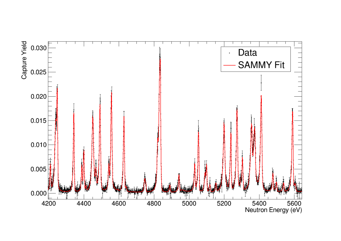
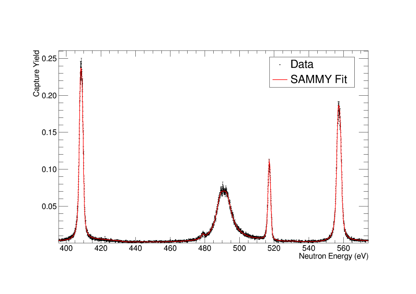
Figure 1: Examples of SAMMY fits of the 73Ge(n,γn,\gamma) neutron capture yield (probability of a neutron capture) obtained with the enriched 73GeO2 sample for two different neutron energy regions.

The resulting capture yield was fitted with the code SAMMY [19], a multilevel, multichannel R-matrix code using Bayes’ method. SAMMY takes into account experimental effects such as Doppler and resolution broadening, self shielding and multiple scattering of neutrons in the sample. SAMMY was used to extract resonance capture kernels kk up to 14 keV neutron energy:

k=g​Γγ​ΓnΓγ+Γn,k=g\frac{\Gamma_{\gamma}\Gamma_{n}}{\Gamma_{\gamma}+\Gamma_{n}}, (2)

where gg denotes the statistical weighting factor (2​J+1(2​I+1)​(2​s+1)\frac{2J+1}{(2I+1)(2s+1)} with JJ being the resonance spin, II the target nucleus spin and ss the neutron spin), Γγ\Gamma_{\gamma} is the radiative width, and Γn\Gamma_{n} is the neutron width. The list of resonance energies and capture kernels up to 14 keV can be found in A. For a few low energy resonances, fitting the natural germanium sample resulted in a much better reproduction of the resonance shape, presumably due to its lower thickness which results in smaller corrections for multiple scattering and self shielding in large resonances. The resonances fitted with the natural germanium samples are clearly marked in the list of resonances of Table 3. Examples of the SAMMY fits of the capture yield are shown in Figure 1.

Above approximately 14 keV neutron energy, the experimental resolution became too low to resolve individual resonances. An averaged cross section was determined from 14 keV to 300 keV neutron energy and self-shielding and multiple scattering corrections were determined in Monte Carlo simulations. These simulations followed the approach of tracing neutrons of a given energy through the sample composed according to the specifications. The trace ended either because the neutron got captured or left the sample. The energy loss in each scattering step was considered, however purely isotropical scattering in the center-of-mass frame was assumed. To determine the correction factors, we used neutron capture and scattering cross sections from ENDF-VIII [10], but scaled the capture cross section to better match the experimentally determined cross sections. Corrections to the capture yield were always smaller than 6%. Calculations using scaled and unscaled capture cross sections, different cross section evaluations, and changes in the sample thickness and geometry indicate that the total systematic uncertainty of the simulations is below 20%, which results in at most 1.2% uncertainty in the capture yield.
The cross sections reconstructed from SAMMY fits in the resolved resonance region below 14 keV, and the unresolved cross sections from 14 to 300 keV are shown in Fig. 2.

Figure 2: (Top) 73Ge(n,γn,\gamma) cross sections reconstructed from SAMMY resonance fits up to 14 keV neutron energy. (Bottom) Averaged cross sections from 14 keV to 300 keV neutron energy and statistical uncertainties.

Combining these two components, we calculated Maxwellian averaged cross sections (MACS) from k​T=5kT=5 to k​T=100kT=100 keV using

M​A​C​S=2π​1(k​T)2⋅∫0∞E​σ​(E)⋅exp⁡(−Ek​T)​d​EMACS=\frac{2}{\sqrt{\pi}}\frac{1}{(kT)^{2}}\cdot\int_{0}^{\infty}E\sigma(E)\cdot\exp{\left(-\frac{E}{kT}\right)}\mbox{d}E (3)

For neutron energies above 300300 keV we used the evaluated ENDF-BV.III cross section [10], scaled by a factor of 1.7 to reproduce the experimental cross section at lower energies. The contribution of this energy range was at most 6% (at k​T=100kT=100 keV) and negligible for k​T<60kT<60 keV. Fig. 3 shows a comparison of the experimental MACS from k​T=5−100kT=5-100 keV, compared to recent evaluations and theoretical predictions. Besides TALYS-1.9 [21] (using default parameters), and MOST-2005 [20] the MACSs are significantly underestimated by all predictions over the entire range of k​TkT values. MACSs recommended by the Kadonis-0.3 database [28], which is used in most nucleosynthesis calculations, are consistently a factor of about 1.5 lower over the entire energy range.

Figure 3: Comparison of the experimental MACS from k​T=5−100kT=5-100 keV with evaluations and theoretical predictions [10, 20, 21, 22, 23, 24, 28]. MOST-2005 [20] and TALYS-1.9 [21] most closely reproduce the experimental values, while all others significantly underestimate the MACS by a factor of up to 2 .

MACSs from k​T=5kT=5 to k​T=100kT=100 keV are listed in Table 1. Table 2 summarises all contributions to the total uncertainty of these stellar cross sections.
In a star, excited states in nuclei may be thermally populated which means that the stellar reaction rate includes neutron capture on both, the ground state and excited states [25]. The cross sections on excited states have been estimated using TALYS-1.9 [21], renormalising average level spacings and average radiative widths to the experimental values obtained in this work (see A), and using the default optical model potential (OMP) [26]. In addition, we investigated the impact on calculated cross sections using a different OMP, i.e. the JKM potential as described in Ref. [27]. Based on this we estimate a factor 1.25 uncertainty for the theoretical neutron capture cross sections on excited states. Consequently, the stellar MACS∗, taking into account neutron capture on excited states, has uncertainties ranging from 6% at k​T=5kT=5 keV, to 14% at k​T=100kT=100 keV. The MACS∗s are also listed in Table 1.

Table 1: Ground state Maxwellian Averaged Cross Sections on 73Ge, and stellar Maxwellian Averaged Cross Sections, taking into account neutron capture on thermally populated excited states.
k​TkT (keV) MACS (mb) MACS∗ (mb)
5 1170±601170\pm 60 1174±691174\pm 69
10 738±38738\pm 38 741±59741\pm 59
20 475±24475\pm 24 470±48470\pm 48
30 362±19362\pm 19 350±40350\pm 40
40 296±15296\pm 15 281±34281\pm 34
50 251±13251\pm 13 235±30235\pm 30
60 219±11219\pm 11 203±27203\pm 27
70 194±10194\pm 10 180±25180\pm 25
80 175.5±8.9175.5\pm 8.9 162±23162\pm 23
90 160.4±8.2160.4\pm 8.2 148±21148\pm 21
100 148.0±7.6148.0\pm 7.6 136±20136\pm 20
Table 2: Uncertainties of Maxwellian averaged 73Ge cross sections
Source Uncertainty (%\%)
Neutron Flux Shape
(<3<3keV; 3 keV-1MeV) <1;3.5<1;3.5
Weighting Functions 3
Normalisation to Au 1
Background Subtraction 1
Sample Enrichment 1
Multiple Scattering and
Self Shielding (>14>14 keV) 1.2
Statistics 0.3
Total 5.1

4 Astrophysical Implications

The MACSs obtained in this work are a factor of about 1.5 larger than MACSs recommended to be used in stellar models, which were based on theoretical and semi-empirical estimates [28]. We have studied the impact of the new stellar neutron capture rate on weak ss process nucleosynthesis using a 15 solar mass (M⊙M_{\odot}) star with a metallicity of Z=0.006Z=0.006 (solar metallicity is Z=0.014Z=0.014 [29]), representative for a site with large overproduction of elemental germanium [30]. In addition we have tested the new rates on main ss process nucleosynthesis in a 2 M⊙M_{\odot} AGB star (Z=0.006). These calculations were performed using the multi-zone post processing code mppnp [31]. It is estimated that the bulk of germanium in the solar system is produced in massive stars, while a small contribution of about 10-20% comes from the main ss process in AGB stars [6].

Figure 4: (Top) Isotopic ratios rel. to 70Ge produced in a 15 M⊙M_{\odot} star prior to Supernova explosion compared to solar system abundances (pink stars). Blue squares show the standard case and are compared to results using the new 73Ge MACS (black circles). The new 73Ge MACS results in a lower 73Ge/70Ge ratio, consistent with the solar system isotopic ratio. (Bottom) Isotopic ratios produced in a 2 M⊙M_{\odot} AGB star.

The top panel in Figure 4 shows the isotopic abundance pattern of germanium isotopes produced in a 15 solar mass star prior to the supernova explosion. The germanium abundances are normalised to 70Ge in each case22 2 70Ge is mainly produced in the ss process and is shielded from rapid neutron capture nucleosynthesis by stable 70Zn.. The new 73Ge(n,γn,\gamma) MACS causes a reduction of the 73Ge abundance by over 30%, thus now reproducing the solar 73Ge/70Ge ratio. 72Ge/70Ge and 74Ge/70Ge are reasonably close to the solar value, considering uncertainties in the associated reaction rates and the fact that other nucleosynthesis processes contribute to a small extent to overall germanium abundances. 76Ge is significantly underproduced compared to solar as this isotope is bypassed by the ss process due to the short half life of 75Ge (terrestrial t1/2=83t_{1/2}=83 min) and is thought to be produced by explosive nucleosynthesis processes (see e.g. [32]). The bottom panel shows the same comparison for a 2M⊙M_{\odot} AGB star. In this case, isotopic ratios are always smaller than solar. Considering that the contribution of AGB stars to solar germanium is only about 10-20%, we can expect that a combination of these two sites would still result in a fair reproduction of the solar germanium abundance pattern. To put firmer constraints on abundances produced in the different stellar sites, high precision MACS data on 70,72,74,76Ge are required; currently, there are no neutron capture data on 72Ge above 4 keV, while uncertainties for recommended MACSs on 74,76Ge at k​T=30kT=30 keV are 8-10% [33, 34]. We expect that new n_TOF data on these isotopes will improve the precision of these MACSs.

Acknowledgements

This work was supported by the Austrian Science Fund FWF (J3503), the Adolf Messer Foundation (Germany), the UK Science and Facilities Council (ST/M006085/1), and the European Research Council ERC-2015-StG Nr. 677497. We acknowledge also support from MSMT of the Czech Republic.

Appendix A Resonance Data

Tables 3 to 7 list capture kernels kk and associated fit uncertainties. The resonance energies have a further systematic uncertainty of 0.06%0.06\% due to the uncertainty in the neutron flight path. The systematic uncertainty on the capture kernels are 3.5% below and 4.8% above 3 keV neutron energy, consisting of uncertainties due to Pulse Height Weighting (3%), normalisation (1%), sample enrichment (1%), and neutron flux (1% below, 3.5% above 3 keV). Neutron capture data by themselves do not always allow a reliable determination of neutron and radiative widths and resonance spins. However, the results from SAMMY fits were consistent with ⟨Γγ⟩≈250\langle\Gamma_{\gamma}\rangle\approx 250 meV for all resonances with ER<8E_{R}<8 keV and Γn/Γγ>>1\Gamma_{n}/\Gamma_{\gamma}>>1; specifically, the maximum-likelihood estimate assuming a Gaussian distribution of radiative widths yielded ⟨Γγ⟩=250​(10)\langle\Gamma_{\gamma}\rangle=250(10) meV and σΓγ=30​(5)\sigma_{\Gamma_{\gamma}}=30(5) meV. Statistical model simulations using the dicebox code [16] indicated only a slightly narrower distribution (15−2015-20 meV). The present experimental value is somewhat higher than literature values of ⟨Γγ⟩=195​(45)\langle\Gamma_{\gamma}\rangle=195(45) meV [35] and 197​(6)197(6) meV [36].

To deduce the statistical resonance properties we construct the so-called bias function, that is the equiprobability for a single resonance at a given neutron energy to be either ss- or pp-wave. The bias function, as shown in Fig. 5, is obtained using the present value of ⟨Γγ⟩\langle\Gamma_{\gamma}\rangle and varying values of the resonance spacing D0D_{0}, the ss-wave neutron strength function S0S_{0} and the pp-wave neutron strength function S1S_{1}. The channel radius was taken in the form R=1.35​A1/3R=1.35A^{1/3}. The comparison of the number of resonances with kk above different multiples (1−5×1-5\times) of the bias function yielded D0=70​(8)D_{0}=70(8) eV, S0=1.90​(25)×10−4S_{0}=1.90(25)\times 10^{-4} and S1=1.1​(3)×10−4S_{1}=1.1(3)\times 10^{-4}; the latter value scales with RR as R2×S1=R^{2}\times S_{1}= const. For comparison, literature values are D0=62​(15)D_{0}=62(15) eV, S0=2.0​(4)×10−4S_{0}=2.0(4)\times 10^{-4} from Ref. [35], and D0=99​(10)D_{0}=99(10) eV, S0=1.66​(40)×10−4S_{0}=1.66(40)\times 10^{-4} from Ref. [36]. Present values were obtained similarly to Ref. [37] from comparison of experimental data with simulations of individual resonance sequences using Wigner distribution of level spacings, Porter-Thomas distribution of reduced neutron widths, and Gaussian distribution of radiative widths.

Refer to caption
Figure 5: Capture kernels kk of 73Ge(n,γn,\gamma) resonances. The solid line shows the bias function (equiprobability for a single resonance at a given neutron energy to be either ss- or pp-wave), constructed to deduce statistical resonance properties.
Table 3: Resonance energies and capture kernels kk of 73Ge(n,γn,\gamma) aResonances fitted with natural germanium sample. ∗Resonances listed in ENDF/B-VIII [10]. bDoublet in ENDF/B-VIII [10].
ERE_{R} (eV) kk (meV) ERE_{R} (eV) kk (meV)
59.34±0.0959.34\pm 0.09 0.0027±0.00050.0027\pm 0.0005 1219.98±0.02∗1219.98\pm 0.02^{*} 110.01±0.98110.01\pm 0.98
79.47±0.0279.47\pm 0.02 0.051±0.0020.051\pm 0.002 1233.15±0.051233.15\pm 0.05 10.56±0.3910.56\pm 0.39
102.73±0.01a,∗102.73\pm 0.01^{a,*} 104.56±0.63104.56\pm 0.63 1276.91±0.051276.91\pm 0.05 3.70±0.133.70\pm 0.13
156.32±0.02156.32\pm 0.02 0.064±0.0030.064\pm 0.003 1316.76±0.03∗1316.76\pm 0.03^{*} 107.28±0.92107.28\pm 0.92
204.17±0.01a,∗204.17\pm 0.01^{a,*} 60.87±0.5460.87\pm 0.54 1358.03±0.02∗1358.03\pm 0.02^{*} 70.77±0.7870.77\pm 0.78
224.83±0.01∗224.83\pm 0.01^{*} 71.82±0.2171.82\pm 0.21 1380.23±0.191380.23\pm 0.19 0.90±0.100.90\pm 0.10
270.90±0.06270.90\pm 0.06 0.075±0.0060.075\pm 0.006 1384.68±0.101384.68\pm 0.10 1.73±0.111.73\pm 0.11
286.68±0.02286.68\pm 0.02 0.206±0.0070.206\pm 0.007 1404.78±0.101404.78\pm 0.10 1.36±0.091.36\pm 0.09
320.70±0.01a,∗320.70\pm 0.01^{a,*} 59.45±0.9259.45\pm 0.92 1462.39±0.081462.39\pm 0.08 2.97±0.152.97\pm 0.15
332.85±0.02a,∗332.85\pm 0.02^{a,*} 88.05±1.3988.05\pm 1.39 1530.62±0.09∗1530.62\pm 0.09^{*} 115.19±3.57115.19\pm 3.57
361.82±0.06361.82\pm 0.06 0.533±0.0460.533\pm 0.046 1540.42±0.101540.42\pm 0.10 3.44±0.223.44\pm 0.22
368.08±0.01∗368.08\pm 0.01^{*} 97.68±0.4197.68\pm 0.41 1549.31±0.141549.31\pm 0.14 3.42±0.333.42\pm 0.33
409.28±0.01∗409.28\pm 0.01^{*} 56.75±0.2556.75\pm 0.25 1552.26±0.071552.26\pm 0.07 6.19±0.246.19\pm 0.24
479.55±0.06479.55\pm 0.06 0.52±0.030.52\pm 0.03 1614.59±0.261614.59\pm 0.26 0.43±0.060.43\pm 0.06
491.55±0.02∗491.55\pm 0.02^{*} 101.31±0.54101.31\pm 0.54 1655.95±0.05∗1655.95\pm 0.05^{*} 118.38±1.26118.38\pm 1.26
517.99±0.01∗517.99\pm 0.01^{*} 12.83±0.1312.83\pm 0.13 1665.35±0.091665.35\pm 0.09 5.87±0.315.87\pm 0.31
558.34±0.01∗558.34\pm 0.01^{*} 71.62±0.3271.62\pm 0.32 1675.01±0.451675.01\pm 0.45 0.55±0.120.55\pm 0.12
668.80±0.04∗668.80\pm 0.04^{*} 0.92±0.030.92\pm 0.03 1716.18±0.041716.18\pm 0.04 18.26±0.3818.26\pm 0.38
693.58±0.04693.58\pm 0.04 0.82±0.030.82\pm 0.03 1751.88±0.191751.88\pm 0.19 0.93±0.090.93\pm 0.09
750.31±0.08750.31\pm 0.08 0.31±0.020.31\pm 0.02 1808.02±0.04∗1808.02\pm 0.04^{*} 109.75±1.15109.75\pm 1.15
762.70±0.02762.70\pm 0.02 3.25±0.063.25\pm 0.06 1843.00±0.081843.00\pm 0.08 3.71±0.183.71\pm 0.18
777.48±0.04777.48\pm 0.04 0.87±0.030.87\pm 0.03 1897.71±0.181897.71\pm 0.18 1.12±0.101.12\pm 0.10
798.47±0.06798.47\pm 0.06 0.42±0.030.42\pm 0.03 1930.82±0.741930.82\pm 0.74 0.30±0.090.30\pm 0.09
816.73±0.22816.73\pm 0.22 0.09±0.010.09\pm 0.01 1952.79±0.05b,∗1952.79\pm 0.05^{b,*} 105.78±1.27105.78\pm 1.27
826.23±0.02826.23\pm 0.02 5.00±0.095.00\pm 0.09 1963.43±0.151963.43\pm 0.15 3.21±0.293.21\pm 0.29
843.31±0.03843.31\pm 0.03 2.96±0.092.96\pm 0.09 2019.34±0.06∗2019.34\pm 0.06^{*} 111.08±1.55111.08\pm 1.55
851.39±0.01∗851.39\pm 0.01^{*} 57.96±0.4757.96\pm 0.47 2104.02±0.112104.02\pm 0.11 3.28±0.203.28\pm 0.20
878.76±0.08878.76\pm 0.08 0.64±0.040.64\pm 0.04 2116.60±0.132116.60\pm 0.13 3.49±0.213.49\pm 0.21
920.46±0.01∗920.46\pm 0.01^{*} 45.96±0.4345.96\pm 0.43 2144.13±0.172144.13\pm 0.17 2.34±0.182.34\pm 0.18
948.07±0.13948.07\pm 0.13 0.30±0.030.30\pm 0.03 2162.03±0.042162.03\pm 0.04 51.19±0.9951.19\pm 0.99
959.17±0.05959.17\pm 0.05 1.49±0.061.49\pm 0.06 2211.39±0.592211.39\pm 0.59 0.48±0.110.48\pm 0.11
1031.14±0.01∗1031.14\pm 0.01^{*} 55.02±0.5955.02\pm 0.59 2216.97±0.512216.97\pm 0.51 0.51±0.100.51\pm 0.10
1059.02±0.011059.02\pm 0.01 72.65±0.6772.65\pm 0.67 2236.71±0.422236.71\pm 0.42 0.99±0.170.99\pm 0.17
1139.18±0.121139.18\pm 0.12 1.93±0.161.93\pm 0.16 2262.54±0.06∗2262.54\pm 0.06^{*} 109.62±1.73109.62\pm 1.73
1148.29±0.03∗1148.29\pm 0.03^{*} 116.35±0.93116.35\pm 0.93 2291.05±0.132291.05\pm 0.13 117.25±4.30117.25\pm 4.30
Table 4: Table 3 continued.
ERE_{R} (eV) kk (meV) ERE_{R} (eV) kk (meV)
2297.90±0.07∗2297.90\pm 0.07^{*} 98.62±4.1198.62\pm 4.11 3431.09±0.663431.09\pm 0.66 6.80±2.476.80\pm 2.47
2321.94±0.072321.94\pm 0.07 15.32±0.5215.32\pm 0.52 3432.30±0.593432.30\pm 0.59 7.24±2.537.24\pm 2.53
2373.25±0.122373.25\pm 0.12 6.25±0.326.25\pm 0.32 3495.70±0.573495.70\pm 0.57 1.45±0.251.45\pm 0.25
2398.90±0.302398.90\pm 0.30 1.42±0.191.42\pm 0.19 3535.63±0.083535.63\pm 0.08 36.88±1.0336.88\pm 1.03
2442.65±0.042442.65\pm 0.04 102.11±1.52102.11\pm 1.52 3565.08±0.343565.08\pm 0.34 3.90±0.413.90\pm 0.41
2531.55±0.242531.55\pm 0.24 2.30±0.232.30\pm 0.23 3579.46±0.083579.46\pm 0.08 34.21±1.0534.21\pm 1.05
2566.67±0.06∗2566.67\pm 0.06^{*} 118.78±1.74118.78\pm 1.74 3628.35±0.343628.35\pm 0.34 3.36±0.363.36\pm 0.36
2624.55±0.142624.55\pm 0.14 7.24±0.447.24\pm 0.44 3657.54±0.163657.54\pm 0.16 19.55±0.9219.55\pm 0.92
2648.04±0.06∗2648.04\pm 0.06^{*} 29.34±0.8529.34\pm 0.85 3674.52±0.073674.52\pm 0.07 99.37±2.3099.37\pm 2.30
2666.79±0.052666.79\pm 0.05 53.87±1.3753.87\pm 1.37 3718.11±0.073718.11\pm 0.07 77.49±1.9577.49\pm 1.95
2688.08±0.052688.08\pm 0.05 107.17±1.92107.17\pm 1.92 3745.16±0.193745.16\pm 0.19 10.03±0.6210.03\pm 0.62
2697.89±0.142697.89\pm 0.14 8.76±0.578.76\pm 0.57 3763.26±0.253763.26\pm 0.25 5.31±0.445.31\pm 0.44
2748.81±0.40∗2748.81\pm 0.40^{*} 2.20±0.302.20\pm 0.30 3809.15±0.593809.15\pm 0.59 4.15±0.974.15\pm 0.97
2763.67±0.292763.67\pm 0.29 2.71±0.312.71\pm 0.31 3812.80±0.463812.80\pm 0.46 3.94±0.853.94\pm 0.85
2776.01±0.062776.01\pm 0.06 47.66±1.0847.66\pm 1.08 3852.87±0.153852.87\pm 0.15 20.94±0.9420.94\pm 0.94
2806.78±0.182806.78\pm 0.18 3.77±0.293.77\pm 0.29 3870.01±0.093870.01\pm 0.09 47.98±1.4047.98\pm 1.40
2821.52±0.362821.52\pm 0.36 1.98±0.221.98\pm 0.22 3993.96±0.293993.96\pm 0.29 8.22±0.718.22\pm 0.71
2903.85±0.182903.85\pm 0.18 5.03±0.355.03\pm 0.35 4002.66±0.164002.66\pm 0.16 5.44±0.585.44\pm 0.58
2924.80±0.142924.80\pm 0.14 11.56±0.6111.56\pm 0.61 4042.61±0.264042.61\pm 0.26 21.00±2.0221.00\pm 2.02
2946.18±0.092946.18\pm 0.09 107.59±1.97107.59\pm 1.97 4053.83±0.254053.83\pm 0.25 155.04±4.40155.04\pm 4.40
2982.63±0.062982.63\pm 0.06 52.53±1.2452.53\pm 1.24 4073.85±0.094073.85\pm 0.09 95.40±3.3995.40\pm 3.39
3005.31±0.85∗3005.31\pm 0.85^{*} 1.03±0.291.03\pm 0.29 4215.88±0.204215.88\pm 0.20 16.14±0.8616.14\pm 0.86
3023.45±0.053023.45\pm 0.05 99.68±1.9599.68\pm 1.95 4246.57±0.254246.57\pm 0.25 103.52±4.11103.52\pm 4.11
3037.63±0.083037.63\pm 0.08 35.20±1.1835.20\pm 1.18 4254.81±0.124254.81\pm 0.12 67.18±3.4967.18\pm 3.49
3044.63±0.633044.63\pm 0.63 1.78±0.401.78\pm 0.40 4349.23±0.10∗4349.23\pm 0.10^{*} 61.07±1.7861.07\pm 1.78
3085.74±0.373085.74\pm 0.37 2.11±0.262.11\pm 0.26 4394.74±0.224394.74\pm 0.22 14.48±0.9314.48\pm 0.93
3133.36±0.573133.36\pm 0.57 1.60±0.291.60\pm 0.29 4406.67±0.144406.67\pm 0.14 30.98±1.4330.98\pm 1.43
3155.23±0.063155.23\pm 0.06 88.69±1.6588.69\pm 1.65 4419.23±0.57∗4419.23\pm 0.57^{*} 3.44±0.533.44\pm 0.53
3214.07±0.153214.07\pm 0.15 8.96±0.528.96\pm 0.52 4458.61±0.134458.61\pm 0.13 118.69±2.81118.69\pm 2.81
3251.24±0.073251.24\pm 0.07 30.04±0.9030.04\pm 0.90 4475.90±0.284475.90\pm 0.28 14.18±1.0114.18\pm 1.01
3264.48±0.433264.48\pm 0.43 1.21±0.201.21\pm 0.20 4499.19±0.114499.19\pm 0.11 98.06±2.5898.06\pm 2.58
3320.71±0.173320.71\pm 0.17 10.34±0.6310.34\pm 0.63 4548.89±0.264548.89\pm 0.26 15.23±1.0915.23\pm 1.09
3361.67±0.103361.67\pm 0.10 46.80±1.4846.80\pm 1.48 4564.61±0.104564.61\pm 0.10 105.98±2.66105.98\pm 2.66
3388.19±0.243388.19\pm 0.24 7.64±0.567.64\pm 0.56 4635.76±0.104635.76\pm 0.10 64.60±2.0064.60\pm 2.00
3414.94±0.213414.94\pm 0.21 61.45±4.5761.45\pm 4.57 4649.59±0.464649.59\pm 0.46 4.28±0.544.28\pm 0.54
Table 5: Table 3 continued.
ERE_{R} (eV) kk (meV) ERE_{R} (eV) kk (meV)
4753.89±0.474753.89\pm 0.47 8.45±1.218.45\pm 1.21 6040.28±0.156040.28\pm 0.15 136.59±4.32136.59\pm 4.32
4759.64±0.474759.64\pm 0.47 7.25±1.077.25\pm 1.07 6075.56±0.16∗6075.56\pm 0.16^{*} 129.63±4.05129.63\pm 4.05
4827.94±0.294827.94\pm 0.29 29.67±1.9629.67\pm 1.96 6136.50±0.656136.50\pm 0.65 9.92±1.189.92\pm 1.18
4837.08±0.354837.08\pm 0.35 54.47±5.9354.47\pm 5.93 6155.03±0.596155.03\pm 0.59 9.35±1.159.35\pm 1.15
4843.10±0.174843.10\pm 0.17 145.17±7.29145.17\pm 7.29 6219.65±0.176219.65\pm 0.17 162.57±4.94162.57\pm 4.94
4898.08±0.504898.08\pm 0.50 6.53±0.756.53\pm 0.75 6241.35±0.166241.35\pm 0.16 92.48±3.8592.48\pm 3.85
4949.81±0.294949.81\pm 0.29 13.67±1.0213.67\pm 1.02 6279.25±0.416279.25\pm 0.41 25.25±2.2025.25\pm 2.20
5039.54±0.225039.54\pm 0.22 23.53±1.2923.53\pm 1.29 6289.68±0.396289.68\pm 0.39 25.43±2.2625.43\pm 2.26
5061.31±0.145061.31\pm 0.14 60.97±2.2960.97\pm 2.29 6327.02±0.416327.02\pm 0.41 27.42±2.2227.42\pm 2.22
5098.11±0.415098.11\pm 0.41 13.75±1.3113.75\pm 1.31 6344.27±0.196344.27\pm 0.19 119.87±4.03119.87\pm 4.03
5106.77±0.22∗5106.77\pm 0.22^{*} 24.34±1.5324.34\pm 1.53 6400.37±1.316400.37\pm 1.31 4.25±1.004.25\pm 1.00
5126.34±0.445126.34\pm 0.44 6.58±0.776.58\pm 0.77 6427.65±0.19∗6427.65\pm 0.19^{*} 54.35±2.4454.35\pm 2.44
5160.94±0.425160.94\pm 0.42 7.58±0.797.58\pm 0.79 6455.88±1.736455.88\pm 1.73 2.93±0.942.93\pm 0.94
5207.94±0.175207.94\pm 0.17 130.66±3.75130.66\pm 3.75 6470.60±0.286470.60\pm 0.28 36.98±2.2736.98\pm 2.27
5221.27±0.295221.27\pm 0.29 2.48±1.212.48\pm 1.21 6485.66±0.396485.66\pm 0.39 22.75±1.8622.75\pm 1.86
5245.99±0.145245.99\pm 0.14 56.01±2.3756.01\pm 2.37 6504.18±0.186504.18\pm 0.18 57.68±2.5257.68\pm 2.52
5281.75±0.135281.75\pm 0.13 124.70±3.34124.70\pm 3.34 6578.25±0.256578.25\pm 0.25 128.75±5.10128.75\pm 5.10
5302.86±0.895302.86\pm 0.89 6.23±1.306.23\pm 1.30 6602.37±0.386602.37\pm 0.38 88.44±10.8388.44\pm 10.83
5312.62±0.235312.62\pm 0.23 32.68±1.9732.68\pm 1.97 6617.24±0.326617.24\pm 0.32 179.31±7.07179.31\pm 7.07
5364.07±0.245364.07\pm 0.24 110.95±4.84110.95\pm 4.84 6626.46±0.686626.46\pm 0.68 102.51±24.32102.51\pm 24.32
5381.79±0.24∗5381.79\pm 0.24^{*} 134.42±5.45134.42\pm 5.45 6741.61±0.526741.61\pm 0.52 2.41±1.202.41\pm 1.20
5419.94±0.125419.94\pm 0.12 134.51±3.65134.51\pm 3.65 6766.29±0.176766.29\pm 0.17 161.31±5.16161.31\pm 5.16
5485.70±0.285485.70\pm 0.28 18.42±1.2718.42\pm 1.27 6826.24±0.856826.24\pm 0.85 8.84±1.198.84\pm 1.19
5506.14±0.385506.14\pm 0.38 9.76±0.899.76\pm 0.89 6866.12±0.226866.12\pm 0.22 109.52±3.86109.52\pm 3.86
5547.03±0.455547.03\pm 0.45 8.88±0.978.88\pm 0.97 6883.56±0.606883.56\pm 0.60 15.78±4.4615.78\pm 4.46
5598.25±0.14∗5598.25\pm 0.14^{*} 103.02±6.29103.02\pm 6.29 6955.68±0.196955.68\pm 0.19 90.86±3.4590.86\pm 3.45
5612.71±0.42∗5612.71\pm 0.42^{*} 9.01±1.059.01\pm 1.05 6973.99±0.616973.99\pm 0.61 11.48±1.5111.48\pm 1.51
5681.92±0.375681.92\pm 0.37 16.51±1.2916.51\pm 1.29 7118.07±0.21∗7118.07\pm 0.21^{*} 81.88±3.2581.88\pm 3.25
5716.47±0.145716.47\pm 0.14 127.76±3.63127.76\pm 3.63 7154.02±0.157154.02\pm 0.15 12.70±4.3812.70\pm 4.38
5764.60±0.235764.60\pm 0.23 142.28±4.41142.28\pm 4.41 7177.26±0.387177.26\pm 0.38 42.10±2.8142.10\pm 2.81
5815.35±0.225815.35\pm 0.22 41.61±2.3641.61\pm 2.36 7221.40±0.187221.40\pm 0.18 127.16±4.61127.16\pm 4.61
5873.42±0.185873.42\pm 0.18 88.73±3.2688.73\pm 3.26 7245.57±0.527245.57\pm 0.52 24.75±2.4224.75\pm 2.42
5927.43±0.035927.43\pm 0.03 9.23±3.449.23\pm 3.44 7290.68±0.277290.68\pm 0.27 138.57±5.11138.57\pm 5.11
5975.46±0.655975.46\pm 0.65 6.73±0.856.73\pm 0.85 7330.83±0.327330.83\pm 0.32 138.82±5.48138.82\pm 5.48
6002.51±0.276002.51\pm 0.27 35.82±2.0235.82\pm 2.02 7370.59±0.247370.59\pm 0.24 90.99±4.0490.99\pm 4.04
Table 6: Table 3 continued.
ERE_{R} (eV) kk (meV) ERE_{R} (eV) kk (meV)
7480.92±0.207480.92\pm 0.20 71.03±3.1071.03\pm 3.10 9038.39±0.259038.39\pm 0.25 129.28±3.32129.28\pm 3.32
7508.04±1.367508.04\pm 1.36 7.98±1.557.98\pm 1.55 9086.33±0.559086.33\pm 0.55 50.07±4.4550.07\pm 4.45
7601.45±0.237601.45\pm 0.23 88.12±3.4888.12\pm 3.48 9097.14±0.929097.14\pm 0.92 22.78±3.6322.78\pm 3.63
7641.78±0.217641.78\pm 0.21 138.99±4.79138.99\pm 4.79 9147.22±1.659147.22\pm 1.65 16.07±2.8016.07\pm 2.80
7756.02±0.817756.02\pm 0.81 13.71±1.8013.71\pm 1.80 9168.58±0.099168.58\pm 0.09 12.59±5.5212.59\pm 5.52
7777.46±0.357777.46\pm 0.35 35.77±2.4535.77\pm 2.45 9191.30±1.049191.30\pm 1.04 26.99±3.8226.99\pm 3.82
7830.29±0.637830.29\pm 0.63 24.88±2.3524.88\pm 2.35 9209.69±0.989209.69\pm 0.98 51.89±9.6751.89\pm 9.67
7862.45±0.507862.45\pm 0.50 107.18±6.19107.18\pm 6.19 9222.47±0.579222.47\pm 0.57 238.54±15.55238.54\pm 15.55
7898.08±0.237898.08\pm 0.23 152.34±6.44152.34\pm 6.44 9266.86±0.619266.86\pm 0.61 46.08±4.3846.08\pm 4.38
7931.41±0.287931.41\pm 0.28 66.22±3.5866.22\pm 3.58 9319.08±0.489319.08\pm 0.48 266.48±10.47266.48\pm 10.47
7971.27±0.317971.27\pm 0.31 132.45±5.25132.45\pm 5.25 9344.08±0.349344.08\pm 0.34 117.15±7.25117.15\pm 7.25
8020.47±0.328020.47\pm 0.32 87.03±5.6487.03\pm 5.64 9363.08±0.069363.08\pm 0.06 16.84±6.8516.84\pm 6.85
8036.76±0.528036.76\pm 0.52 29.75±2.7829.75\pm 2.78 9490.32±0.279490.32\pm 0.27 171.80±6.02171.80\pm 6.02
8099.71±0.268099.71\pm 0.26 172.56±5.65172.56\pm 5.65 9545.52±1.199545.52\pm 1.19 16.24±3.1616.24\pm 3.16
8148.02±0.468148.02\pm 0.46 38.81±2.8638.81\pm 2.86 9559.05±0.969559.05\pm 0.96 24.89±3.5824.89\pm 3.58
8180.99±0.298180.99\pm 0.29 89.16±4.3989.16\pm 4.39 9575.23±0.839575.23\pm 0.83 25.93±3.4425.93\pm 3.44
8329.05±0.378329.05\pm 0.37 41.98±2.7741.98\pm 2.77 9626.54±0.309626.54\pm 0.30 114.82±5.06114.82\pm 5.06
8349.70±0.188349.70\pm 0.18 7.18±3.337.18\pm 3.33 9707.30±1.769707.30\pm 1.76 10.11±3.1010.11\pm 3.10
8417.95±0.11∗8417.95\pm 0.11^{*} 3.14±1.583.14\pm 1.58 9728.35±0.389728.35\pm 0.38 100.08±5.62100.08\pm 5.62
8442.04±0.918442.04\pm 0.91 12.93±1.9612.93\pm 1.96 9802.54±0.859802.54\pm 0.85 105.66±9.33105.66\pm 9.33
8488.63±2.318488.63\pm 2.31 84.68±17.7384.68\pm 17.73 9816.46±0.479816.46\pm 0.47 98.85±8.4298.85\pm 8.42
8507.36±1.158507.36\pm 1.15 60.74±15.5360.74\pm 15.53 9863.34±0.749863.34\pm 0.74 22.36±2.8022.36\pm 2.80
8543.29±0.548543.29\pm 0.54 25.55±2.6325.55\pm 2.63 9965.97±0.129965.97\pm 0.12 28.25±10.9428.25\pm 10.94
8587.34±0.008587.34\pm 0.00 102.17±0.00102.17\pm 0.00 9994.54±0.749994.54\pm 0.74 76.06±8.5976.06\pm 8.59
8608.28±0.118608.28\pm 0.11 27.93±10.6827.93\pm 10.68 10009.71±0.4010009.71\pm 0.40 160.40±8.59160.40\pm 8.59
8643.80±0.138643.80\pm 0.13 6.27±2.986.27\pm 2.98 10036.48±1.2310036.48\pm 1.23 26.30±4.9426.30\pm 4.94
8675.02±0.308675.02\pm 0.30 86.79±4.4786.79\pm 4.47 10044.32±0.6710044.32\pm 0.67 55.82±7.5555.82\pm 7.55
8713.59±0.338713.59\pm 0.33 113.27±5.55113.27\pm 5.55 10154.46±0.4410154.46\pm 0.44 99.85±5.4999.85\pm 5.49
8765.54±0.428765.54\pm 0.42 42.84±3.0942.84\pm 3.09 10208.17±0.4010208.17\pm 0.40 154.81±6.70154.81\pm 6.70
8810.89±0.388810.89\pm 0.38 68.27±4.1068.27\pm 4.10 10356.43±0.4410356.43\pm 0.44 98.20±5.0598.20\pm 5.05
8833.81±0.628833.81\pm 0.62 19.05±1.9619.05\pm 1.96 10414.95±0.6710414.95\pm 0.67 81.57±6.9381.57\pm 6.93
8864.19±0.128864.19\pm 0.12 13.46±5.9313.46\pm 5.93 10443.78±0.4010443.78\pm 0.40 212.08±10.08212.08\pm 10.08
8905.57±1.258905.57\pm 1.25 10.06±1.8410.06\pm 1.84 10474.67±1.4410474.67\pm 1.44 13.90±2.6213.90\pm 2.62
8921.97±1.168921.97\pm 1.16 11.69±2.0111.69\pm 2.01 10511.30±1.0010511.30\pm 1.00 10.38±3.2210.38\pm 3.22
9000.02±0.31∗9000.02\pm 0.31^{*} 89.86±4.7989.86\pm 4.79 10580.16±1.2010580.16\pm 1.20 44.98±8.3144.98\pm 8.31
Table 7: Table 3 continued.
ERE_{R} (eV) kk (meV) ERE_{R} (eV) kk (meV)
10598.22±1.1010598.22\pm 1.10 138.91±18.94138.91\pm 18.94 11967.33±0.5211967.33\pm 0.52 170.17±9.65170.17\pm 9.65
10613.21±0.6110613.21\pm 0.61 123.79±14.39123.79\pm 14.39 12030.65±0.9012030.65\pm 0.90 31.06±3.0831.06\pm 3.08
10683.28±0.6110683.28\pm 0.61 86.73±6.6086.73\pm 6.60 12100.52±0.6012100.52\pm 0.60 117.07±6.83117.07\pm 6.83
10702.36±0.1010702.36\pm 0.10 13.76±6.1713.76\pm 6.17 12180.40±1.1512180.40\pm 1.15 35.23±3.6235.23\pm 3.62
10746.07±0.7110746.07\pm 0.71 112.63±11.42112.63\pm 11.42 12280.12±1.0712280.12\pm 1.07 72.49±6.5972.49\pm 6.59
10767.05±1.5810767.05\pm 1.58 56.25±16.9156.25\pm 16.91 12323.72±0.6612323.72\pm 0.66 69.06±5.9469.06\pm 5.94
10776.24±1.1210776.24\pm 1.12 233.72±29.00233.72\pm 29.00 12444.22±1.0012444.22\pm 1.00 50.39±5.3250.39\pm 5.32
10801.25±0.9110801.25\pm 0.91 42.83±7.0242.83\pm 7.02 12558.97±0.6312558.97\pm 0.63 113.80±7.86113.80\pm 7.86
10851.47±0.4210851.47\pm 0.42 155.87±8.83155.87\pm 8.83 12586.55±0.8812586.55\pm 0.88 73.87±6.9973.87\pm 6.99
10890.06±0.4710890.06\pm 0.47 183.52±9.28183.52\pm 9.28 12664.81±0.4212664.81\pm 0.42 146.51±8.08146.51\pm 8.08
10945.27±0.6910945.27\pm 0.69 33.74±3.1333.74\pm 3.13 12757.68±0.5912757.68\pm 0.59 168.20±9.74168.20\pm 9.74
11085.56±0.8511085.56\pm 0.85 34.87±3.9434.87\pm 3.94 12849.82±0.5512849.82\pm 0.55 236.74±10.65236.74\pm 10.65
11136.11±0.8111136.11\pm 0.81 68.18±8.2668.18\pm 8.26 12908.84±1.0812908.84\pm 1.08 35.87±4.1935.87\pm 4.19
11156.54±1.1611156.54\pm 1.16 144.45±39.12144.45\pm 39.12 12979.04±0.9612979.04\pm 0.96 52.03±6.6052.03\pm 6.60
11161.78±1.0811161.78\pm 1.08 178.91±40.17178.91\pm 40.17 13010.31±1.8113010.31\pm 1.81 95.95±18.8895.95\pm 18.88
11211.63±0.4711211.63\pm 0.47 107.58±6.76107.58\pm 6.76 13029.01±1.3513029.01\pm 1.35 107.14±18.96107.14\pm 18.96
11240.54±1.0511240.54\pm 1.05 19.73±2.9119.73\pm 2.91 13069.80±1.3813069.80\pm 1.38 46.53±7.2446.53\pm 7.24
11317.49±1.8511317.49\pm 1.85 64.94±8.6764.94\pm 8.67 13113.37±1.3213113.37\pm 1.32 28.32±3.8928.32\pm 3.89
11343.57±0.8811343.57\pm 0.88 58.18±7.7058.18\pm 7.70 13234.12±0.5313234.12\pm 0.53 138.79±7.45138.79\pm 7.45
11360.04±0.6211360.04\pm 0.62 63.63±6.0463.63\pm 6.04 13289.11±0.6513289.11\pm 0.65 74.27±11.6774.27\pm 11.67
11409.51±1.0311409.51\pm 1.03 40.34±4.5040.34\pm 4.50 13350.23±1.6613350.23\pm 1.66 28.49±4.0028.49\pm 4.00
11441.92±0.4911441.92\pm 0.49 97.07±5.9797.07\pm 5.97 13384.20±1.2613384.20\pm 1.26 50.88±6.1350.88\pm 6.13
11482.53±1.5511482.53\pm 1.55 16.56±3.2116.56\pm 3.21 13407.66±1.5713407.66\pm 1.57 50.26±8.1050.26\pm 8.10
11526.36±0.0711526.36\pm 0.07 15.46±6.1715.46\pm 6.17 13425.24±0.7813425.24\pm 0.78 121.41±11.21121.41\pm 11.21
11543.91±0.1711543.91\pm 0.17 14.97±6.4214.97\pm 6.42 13515.10±1.3113515.10\pm 1.31 85.01±9.5685.01\pm 9.56
11570.35±0.7211570.35\pm 0.72 76.14±6.3376.14\pm 6.33 13551.33±0.5213551.33\pm 0.52 280.04±14.04280.04\pm 14.04
11597.57±0.9811597.57\pm 0.98 40.01±4.3140.01\pm 4.31 13655.16±0.8313655.16\pm 0.83 53.61±5.6053.61\pm 5.60
11618.38±0.9311618.38\pm 0.93 32.60±3.9932.60\pm 3.99 13700.20±0.6813700.20\pm 0.68 102.99±7.16102.99\pm 7.16
11675.00±0.6811675.00\pm 0.68 116.44±9.37116.44\pm 9.37 13740.58±1.3613740.58\pm 1.36 27.18±3.8527.18\pm 3.85
11700.46±0.6411700.46\pm 0.64 126.12±9.90126.12\pm 9.90 13767.27±1.4913767.27\pm 1.49 32.44±4.8532.44\pm 4.85
11795.03±0.6411795.03\pm 0.64 118.44±7.41118.44\pm 7.41 13796.78±1.0713796.78\pm 1.07 48.92±5.1048.92\pm 5.10
11821.08±1.4311821.08\pm 1.43 20.32±3.3920.32\pm 3.39 13857.56±0.7613857.56\pm 0.76 133.77±10.78133.77\pm 10.78
11855.97±1.5811855.97\pm 1.58 21.54±3.5621.54\pm 3.56 13900.68±1.5013900.68\pm 1.50 138.73±13.17138.73\pm 13.17
11883.77±1.4811883.77\pm 1.48 34.50±5.3634.50\pm 5.36 13940.97±1.1113940.97\pm 1.11 88.29±10.8388.29\pm 10.83
11911.03±0.4511911.03\pm 0.45 188.90±10.26188.90\pm 10.26 13967.49±0.7213967.49\pm 0.72 154.22±10.11154.22\pm 10.11

References

  • [1] J. G. Peters, Astroph. J. 154, 225 (1968).
  • [2] R. G. Couch, A. B. Schmiedekamp and W. D. Arnett, Astroph. J. 190, 95 (1974).
  • [3] S. A. Lamb, W. M. Howard, J. W. Truran, and I. Iben, Astroph. J. 217, 213 (1977).
  • [4] C. M. Raiteri, M. Busso, G. Picchio, and R. Gallino, Astroph. J. 371, 665 (1991).
  • [5] C. M. Raiteri, M. Busso, G. Picchio, R. Gallino, and L. Pulone, Astroph. J. 367, 228 (1991).
  • [6] M. Pignatari, R. Gallino, M. Heil, M. Wiescher, F. Käppeler, F. Herwig, S. Bisterzo, Astroph. J. 710, 1557-1577 (2010).
  • [7] N. Nishimura, et al., MNRAS 469, 1752 (2017).
  • [8] K. Maletski, L.B. Pikelner, I.M. Salamatin, E.I. Sharapov, At. Energ. USSR 24,173 (1968).
  • [9] J.A. Harvey, M. Hockaday, EXFOR Entry 13770.004.
  • [10] D.A. Brown, et al., Nucl. Data Sheets 148, 1-142 (2018).
  • [11] C. Guerrero, and the n_TOF collaboration, Eur. Phys. J. A 48, 29(2012).
  • [12] C. Massimi, et al., J. Kor. Phys. Soc. 59, 1689 (2011).
  • [13] R.L. Macklin and R.H. Gibbons, Phys. Rev. 159, 1007 (1967).
  • [14] U. Abbondanno, and the n_TOF collaboration, Nucl. Instrum. Methods Phys. Res. A 521, 454–467 (2004).
  • [15] S. Agostinelli et al. (Geant4 Collaboration), Nucl. Instr. Meth. Phys. Res. A 506, 250 (2003).
  • [16] F. Bečvář, Nucl. Instr. Meth. A417, 434 (1998).
  • [17] M. Sabaté-Gilarte, M. Barbagallo, and the n_TOF Collaboration. n_TOF Collaboration Meeting, Catania, May 2016.
  • [18] M. Barbagallo, et al., Eur. Phys. J. A 49, 156 (2013).
  • [19] N.M. Larson, Technical report ORNL/TM-9179/R8, Updated users guide for SAMMY: Multilevel R-matrix fits to neutron data using Bayes’ equations, Oak-Ridge National Laboratory, Oak Ridge, TN, USA (2008).
  • [20] S. Goriely, Hauser-Feshbach rates for neutron capture reactions (version 8/29/2005), http://www-astro.ulb.ac.be/Html/hfr.html.
  • [21] A.J. Koning, et al., TALYS-1.9, online at www.talys.eu.
  • [22] A.J. Koning, et al., Nucl. Data Sheets 113, 2841 (2012) (https://tendl.web.psi.ch/tendl_2015/tendl2015.html).
  • [23] K. Shibata, et al., J. Nucl. Sci. Technol. 48, 1 (2011).
  • [24] JEFF-3.2 (2014) available online: http://www.oecd-nea.org/dbforms/data/eva/evatapes/jeff_32/.
  • [25] T. Rauscher, Astroph. J. Letters 755, L10 (2012); Astroph. J. Letters 864, L40 (2018).
  • [26] A.J. Koning and J.P. Delaroche, Nucl. Phys. A 713, 231 (2003).
  • [27] E. Bauge, J.P Delaroche, and M. Girod, Phys. Rev. C63, 024607 (2001).
  • [28] I. Dillmann, R. Plag, F. Käppeler, and T. Rauscher, EFNUDAT Fast Neutrons - scientific workshop on neutron measurements, theory & applications, JRC-IRMM (2009); online at http://www.kadonis.org.
  • [29] M. Asplund, et al., Ann. Rev. Astron. Astrophys. 47, 481 (2009).
  • [30] C. Ritter, et al., MNRAS 480, 538 (2018).
  • [31] F. Herwig, et al., PoS(NIC X)023 (2008).
  • [32] A. Perego, et al., MNRAS 443, 3134 (2014).
  • [33] KADoNis Database Revision 1.0 (test version).
  • [34] J. Marganiec, et al., Phys. Rev. C79, 065802 (2009).
  • [35] R. Capote, et al, Nucl. Data Sheets 110, 3107 (2009).
  • [36] S. Mughabghab, Atlas of Neutron Resonances, 5th Edition, Elsevier, 2006.
  • [37] J. Lerendegui-Marco, et al, Phys. Rev. C97, 024605 (2018).