Effect of lensing magnification on type Ia supernova cosmology2018Effect of lensing magnification on type Ia supernova cosmology–References
Abstract
Effect of gravitational magnification on the measurement of distance modulus of type Ia supernovae is presented. We investigate a correlation between magnification and Hubble residual to explore how the magnification affects the estimation of cosmological parameters. We estimate magnification of type Ia supernovae in two distinct methods: one is based on convergence mass reconstruction under the weak lensing limit and the other is based on the direct measurement from galaxies distribution. Both magnification measurements are measured from Subaru Hyper Suprime-Cam survey catalogue. For both measurements, we find no significant correlation between Hubble residual and magnification. Furthermore, we correct for the apparent supernovae fluxes obtained by Supernova Legacy Survey 3-year sample using direct measurement of the magnification. We find and for supernovae samples corrected for lensing magnification when we use photometric redshift catalogue of Mizuki, while and for DEmP photo-z catalogue. Therefore, we conclude that the effect of magnification on the supernova cosmology is negligibly small for the current surveys; however, it has to be considered for the future supernova survey like LSST.
Keywords:
keyword1 – keyword2 – keyword31 introduction
Type Ia supernova (SN) is a useful tool to probe cosmological model. The absolute magnitude of SN at the cosmological distance is empirically well calibrated with the local SN and due to the brightness, it can be observed up to high redshift . Several SNe surveys over wide range of redshift are carried out in this two decades for cosmological study (Riess et al. 1999; Filippenko et al. 2001; Astier et al. 2006; Frieman et al. 2008; Dawson et al. 2009; Grogin et al. 2011). Since late 1990s, distant SNe Ia surveys have suggested that the Universe is accelerating expanding (Garnavich et al. 1998; Riess et al. 1998; Perlmutter et al. 1999). The accelerating expansion of the Universe requires the existence of dark energy within the context of general relativity or possible extension of the theory of gravity. Lately, other cosmological probes such as cosmic microwave background (Komatsu et al. 2011; Planck Collaboration et al. 2015, CMB;) and baryon acoustic oscillation (Percival et al. 2010; Alam et al. 2017, BAO;) also prefer the cosmological model consistent with what obtained by the SNe observations.
With the SNe Ia, we can constrain the cosmological models by use of distance modulus over their redshifts by comparing the difference between apparent and absolute magnitude to the theoretical prediction which simply can be described by the luminosity distance (Astier et al. 2006; Kessler et al. 2009; Guy et al. 2010; Suzuki et al. 2012; Ganeshalingam et al. 2013; Rest et al. 2014). When we look at the distance modulus around the best predicted curve, it is prominently observed that there is a large scatter around the prediction. Apart from the statistical fluctuation, the scatters originate both from intrinsic diversity of the SNe, and the flux magnification due to the gravitational lensing by the foreground mass distribution. The SNe fluxes are amplified when the local matter density along the line of sight of SN is higher than average, while they are diminished at lower density regions. Several attentions have been paid to the effect of gravitational lensing on the measurement of the distance modulus of SNe Ia. Frieman 1996 found that the dispersion of apparent magnitude due to weak lensing by large scale structure is at source redshift in the flat CDM model. Hamana & Futamase 2000 considered the lensing dispersion in peak magnitude of SNe and found that the dispersion at redshift . Gunnarsson et al. 2006 made mock galaxy data to investigate the lensing dispersion and showed that a correction of lensing effect can reduce the lensing dispersion from about 7% to 3% for a source at . Hada & Futamase 2016 predicted that the lensing dispersion of SNe Ia data sets is about 0.03 mag at by using galaxies with virial mass .
The expected effect of gravitational lensing on the SN flux has been studied by using numerical simulations. Wambsganss et al. 1997 found that the gravitational lensing effect causes the magnitude dispersion of source objects of 0.04 mag at redshift . Jönsson et al. 2009 have found that with the mock simulation assuming SNLS-like survey can reduce the scatter on the SNe fluxes by 4% when the intrinsic scatter is 0.13 mag and that the errors on and can be reduced by . The probability distribution functions (PDFs) of lensing magnification are also investigated by simulations. Wang 1999 proposed a fitting formula of PDF for the magnification as the function of and the parameter representing the inhomogeneous density distribution. Takahashi et al. 2011 studied PDFs of convergence, shear and magnification by performing N-body ray-tracing simulations to find the relation between mean and variance of convergence and found the analytic formulae of PDFs well fit the simulated ones.
Also there have been several attempts for correcting the magnification applied to the actual observed data. Jönsson et al. 2007 used 26 SNe in GOODS fields to study the correlation between lensing magnification and residual magnitude of SNe. They found that the correlation coefficient between them is with rather weak significance of , which is consistent with what expected given the small number of samples. Kronborg et al. 2010 used deep images of CFHTLS with SNLS SNe and found a lensing signal at significance. Smith et al. 2014 calculated convergence by using SDSS-II galaxy sample for each SNe Ia from SDSS-II and BOSS surveys under the weak lensing approximation and found a correlation between convergence and Hubble residual at significance.
In this paper, we investigate magnification of SNe Ia fluxes using HSC galaxy photometric catalog. We estimate magnification by two distinct methods: one measures convergence by mass reconstruction using galaxy shape catalog under the weak lensing approximation. The other method measures magnification directly from galaxy distribution assuming that galaxy resides dark matter halo with an NFW profile without assuming the weak lensing regime. We also investigate the impact of magnification effect on the cosmological parameter estimation by comparing the results with and without the magnification correction to the distance modulus.
The paper is organized as follows. In section 2, we describe the SNe Ia and galaxy data sets we use. In section 3, we describe our simulation used for evaluating the expected magnification. In section 4, we overview the measurement of the distance modulus. In section 5, we revisit the measurement of the magnification based on the shape catalog and then introduce our new estimator which better expresses the magnification. In section 6, we present the results of magnification by two different estimators and the effect of magnification on the parameter estimation. In section 7, we give a conclusion and summary.
2 Data sets
2.1 Supernova Legacy Survey 3-year sample
We use Supernova Legacy Survey (SNLS) 3-year data products for SNe Ia analysis (Guy et al. 2010). SNLS program is carried out from 2003 to 2008 to detect high-redshift SNe Ia which are then used for constraining the cosmological model such as dark energy. SNLS consists of two distinct observations: one is photometric cadence survey to measure the light curves of the SNe and the another is spectroscopic survey to confirm the redshift and the spectral type of the detected transient objects. SNLS uses the deep images of MegaCam on Canada-France-Hawaii Legacy Survey (CFHTLS), which cover four distinct patches of the sky. These patches are named D1 to D4 and roughly one square degree area for each. The images are taken in four broad band filters to obtain the color information of the SN. The SNe spectra are taken by Very Large Telescope (VLT), Gemini-North and South and Keck telescopes.
SNLS 3-year data sets are used to estimate cosmological parameters. From SNLS3 only, Guy et al. 2010 find and Conley et al. 2011 extend the analysis to time varying dark energy model to find the equation-of-state parameter . A joint analysis of SNLS3 with BAO from Sloan Digital Sky Survey (SDSS) and CMB from 7 year Wilkinson Microwave Anisotropy Probe (WMAP) yields and for the flat Universe model (Sullivan et al. 2011). SNLS3 data sets are also used to constrain SNe Ia progenitors (Bianco et al. 2011) and to improve the accuracy of photometric calibration (Betoule et al. 2013).
Guy et al. 2010 use two empirical methods for modelling SN Ia light curve: SALT2 (Guy et al. 2007), and SiFTO (Conley et al. 2008). The main difference between two is in the way of modeling the color correction term , defined in equation (11). The SALT2 uses a single color to constrain from the light curve fitting while SiFTO uses 5 filters.
Following Guy et al. 2010, we make a clean sample of SNe by removing SNe having poorly constrained light curve, extreme property among the diversity of type Ia SNe, peak color is significantly affected by dust extinction in the host galaxy or the number of colors obtained is significantly smaller than what has been scheduled. We also exclude outliers in the Hubble residual and finally we obtain 231 SNe.
2.2 Hyper Suprime-Cam
Hyper Suprime-Cam (HSC), is the wide field optical imaging camera installed on the prime focus of the Subaru Telescope (Miyazaki et al. 2018; Komiyama et al. 2018; Kawanomoto et al. 2018; Furusawa et al. 2018). The field of view of the camera is 1.77 square degrees and the pixel size is 0.17 arcsecs. With this gigantic camera and the good quality of seeing and transparency, HSC collects the precise shape and photometry of galaxies. The HSC survey is a Subaru Strategic Program (SSP) which consists of three different layers, wide (1400 [deg2]), deep (27.5 [deg2]) and ultra-deep (3.5 [deg2]), with five broad-band filters, g,r,i,z and y. Deep and ultra-deep layers have additional four narrow-band filters (Aihara et al. 2018).
In this paper, we use photometric redshift catalogs for S17A release from deep and ultra-deep layers and S16A galaxy shape catalog from wide layers overlapped with deep and ultra-deep layers (Mandelbaum et al. 2018). The shape of the galaxies are measured based on the re-Gaussianization method (Hirata & Seljak 2003), applied to the coadd of -band images in the full-depth-full-color (FDFC) regions where all the broad-band data reaches to the target depthes (26 PSF magnitude in -band). Interested readers should refer to Mandelbaum et al. 2008 for more detail about the shape catalog.
We use two different photometric redshift catalogs: one from template fitting, Mizuki (Tanaka 2015) and the other based on the empirical method, DEmP (Hsieh & Yee 2014). Both codes are calibrated with the publicly available spectroscopic redshifts, grism/prism redshift and high quality photometric redshift in COSMOS (Laigle et al. 2016). Mizuki derives photometric redshift and stellar mass simultaneously by fitting the 5 band photometry to the expected galaxy templates, while the DEmP derives redshift by looking for 40 nearest counterpart of the spectroscopic redshift in color-magnitude multi-dimensional space. DEmP also finds the stellar mass by the same way but in the COSMOS high precision photo-z catalog in color-magnitude-redshift multi-dimensional space. The photometric redshift accuracy and methodology are summarized in Tanaka et al. 2018.
The HSC and SNLS fields are partially overlapped at D1, D2 and D3 fields, which contains 158 sample selected SNe. We further remove 5 SNe located near the very bright stars, with the separation closer than 0.8 arcmins, because the photometry of galaxies in the vicinity of bright star can be contaminated by the star and brings large systematic errors on the photometric redshifts. The example of the SN near the bright star is shown in the left panel of Figure 2. Eventually, the number of SNe we use in our analysis is 153.
3 Simulation
In this section, we describe the expectation of the amount of magnification due to the large-scale structure both from numerical simulation and the standard CDM prediction.
3.1 Specifications of the suite of simulation
We use the all-sky multiple lens plane ray-trace simulation data sets (Takahashi et al. 2017). They first make high-resolution N-body simulations with 14 different boxes at light cone output placed around the observer. The box sizes are from 450 to 6300 Mpc with interval of Mpc. Redshift of each output corresponds to the radial distance from the observer at centre. The number of particles included in each box is fixed to so that the mass resolution is higher at lower redshift. Each cubic box is divided into three spherical shells separating Mpc and the particle positions are projected onto the shells. The entire sky is segmentalized by the Healpix pixels into equal area pixels, and all the particle positions are replaced by the central position of the nearest pixel. The projected density can be used to compute the deflection angle and then complete a multiple lens approximated ray-tracing simulation. We use , which corresponds to the pixel of 0.86 arcmins on a side up to redshift .
3.2 Expectation from the simulation and CDM model
In this subsection, we estimate analytic from CDM model and from N-body simulation. Here we assume the flat Universe. The matter perturbation along the line of sight makes the image of the source object distorted. The convergence at given sky position along the line of sight is approximated by (Bartelmann & Schneider 2001),
| (1) |
where is the comoving distance from us to the source object, is three dimensional overdensity of matter distribution and . The power spectrum of the convergence is obtained by using the Limber’s equation in the Fourier space (Limber 1954; Kaiser 1992),
| (2) |
where is the matter power spectrum.
In order to compare the theoretical prediction with the simulation, we smooth the convergence field with two dimensional Gaussian window function in the Fourier space,
| (3) |
where is a smoothing scale. Since we use the simulation with whose pixel area is arcmin2, we adopt arcmin so that satisfies . Then the power spectrum of the smoothed convergence is rewritten as
| (4) |
Assuming the weak gravitational lens, the magnification can be approximated by equation (17). Therefore, the smoothed power spectrum is equal to .
The corresponding two-point angular correlation function is related to with (Peebles 1973),
| (5) |
where is the Legendre polynomial. Then the root mean square of is readily obtained as
| (6) |
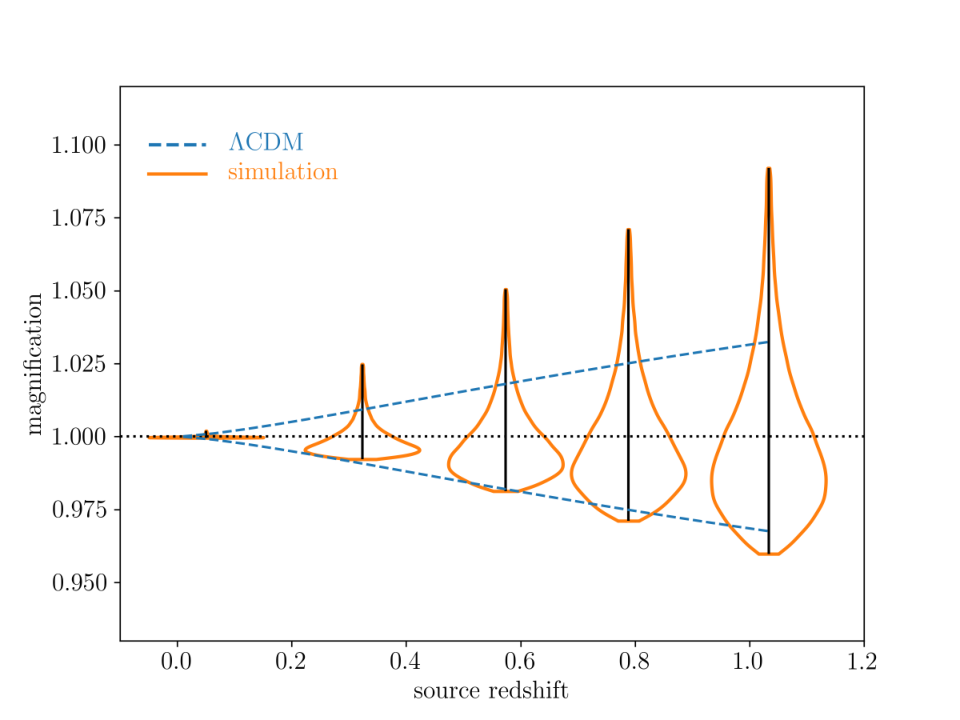
Figure 1 shows the dependence of source redshift on magnification predicted by CDM model and simulation. At , CDM model predicts , while from the simulation, we obtained 68% confidence region as , which is slightly smaller than that from CDM prediction.
4 Distance modulus for type Ia supernovae
In this section, we overview the methodology of constraining dark energy model from the distance modulus of type Ia supernovae.
4.1 distance modulus and dark energy
Distance modulus of SN Ia can be used as the probe of the cosmological model. The distance modulus is a relation between observed and absolute magnitude which is given by
| (7) |
where and are apparent magnitude and absolute magnitude respectively. In the case of type Ia SN, we can readily estimate the absolute magnitude by the method described in 4.2. The observed distance modulus can then be compared with the theoretical prediction to constrain the cosmological models. The luminosity distance in Eq. (7) can be described as
| (8) |
where is the radial coordinate which can be related with comoving distance as
| (9) |
depending on the spatial curvature of the Universe, . The comoving distance is an integral of the inverse of Hubble parameter,
| (10) |
where is the current Hubble parameter, and are the current density parameters of the matter, curvature, and dark energy respectively. In this paper, we consider the time-dependent dark energy model which can be parametrized by equation of state parameter .
4.2 light curve of the type Ia supernova
Type Ia SNe are quite accurate standard candles in the Universe so that they can be used to constrain the model of dark energy. Although the binary system of their progenitor evolution is still not clear, SN Ia is a thermonuclear explosion of C+O white dwarf in a binary system (Maeda & Terada 2016, e.g.). As the SNe Ia explosion mechanism and the maximum progenitor mass is limited by the Chandrasekhar mass, the SNe Ia have a uniform luminosity at the peak of the light curve. Although there is some diversity in the intrinsic feature of the SN Ia, the width of the light curve is well correlated with the maximum luminosity and the diversity can be fairly well corrected by the empirical relation. The correction is required to measure the distance accurate enough to constrain the cosmological parameters. Phillips 1993 investigated the relation between decline rate of SN Ia light curve and peak luminosity, and found that the light curve of brighter SN declines slower than the fainter one. Riess et al. 1995 applied the relation to distance modulus and obtained smaller dispersion of Hubble residual by a factor 2.4 than the dispersion without correction. In addition to this shape-luminosity relation, the relation between luminosity and color is also used to correct the absolute magnitude. Wang et al. 2005 found that the peak luminosity is linearly correlated with color and that the correction can reduce the dispersion to 0.18 mag in band.
From the light curve fitting by SiFTO, rest-frame magnitude , shape parameter and color parameter are obtained. Then the corrected distance modulus of SN Ia is defined as (Guy et al. 2010),
| (11) |
The measurement uncertainty is , where
| (12) |
and is the covariance matrix of (Guy et al. 2007).
4.3 current constraints
Now we find the best-fitting parameters with the maximum likelihood,
| (13) |
where represents a cosmological parameter vector, and is SN redshift. The additional variance accounts for all the sources of diversity of SNe beyond the correction of shape and color and we adopt the value of as suggested in Guy et al. 2010. We use the light curve parameters and obtained by the SiFTO model for each SN. Under the assumption of flat Universe, the parameters we estimate are and constant equation of state parameter for dark energy together with the nuisance parameters, and .
When we estimate parameters, we have to correct the Malmquist bias (Malmquist 1936) with respect to distance modulus. The analysis of the bias with SNLS data sets is studied by Perrett et al. 2010. They use Monte Carlo simulations and estimate the relation between source redshift at and the dispersion of magnitude due to Malmquist bias. We correct the bias by subtracting the value estimated by this relation at each SN redshift from distance modulus.
5 Estimation of magnification
 |
 |
In this section, we first revisit the estimate of the magnification which is based on the weak lensing convergence and is widely used in the literature. Then we describe our new estimator which may better describe the magnification. In this paper we consider two different measurements of the magnification for comparison.
5.1 Convergence measure
We describe the estimator from convergence which is reconstructed by the shape of galaxies distorted (Oguri et al. 2018). The gravitational lensing distorts the image of the source galaxies. This effect is described by the Jacobian matrix when the lensed images are projected back to the source plane,
| (14) |
where we define convergence and complex shear in terms of lensing potential ,
| (15) |
The magnification can then be
| (16) |
Here we work within the weak lensing regime. In the limit of weak lensing where , the magnification can be approximated as
| (17) |
The convergence can be related to the shear by
| (18) |
where is a Fourier counterpart of the kernel function, (Kaiser & Squires 1993). Since equation (18) diverges on small scales, we apply a two-dimensional Gaussian filter with smoothing scale ,
| (19) |
We use HSC shear catalog (Mandelbaum et al. 2018) with the smoothing scale arcmins to reconstruct the convergence maps. Since the HSC shear catalog only overlaps with D1 field, the total number of SNe used for this convergence measurement is limited to 52. The total number of galaxies used is 104,303. We use photo-z catalog obtained by Mizuki code (Tanaka et al. 2018). For each SN, we reconstruct the surface density using galaxies within SNLS D1 field then obtain convergence along the lines of sight of SNe from the convergence maps. In the calculation, we use galaxy whose redshift satisfies
| (20) |
After applying this sample selection, we have average galaxy number density for and for .
5.2 Direct measure
5.2.1 Lensing estimation
Here we propose to measure the magnification in an alternative manner. In this method, we consider that the SN flux is magnified at the position of foreground galaxies in a single lens approximation. We also assume that the galaxy has a spherically symmetric profile, . The projected mass of the galaxy along the line of sight is then,
| (21) |
where and are centric comoving radius along and perpendicular to the line of sight. The convergence and two shear components induced by the mass associated with the galaxy are then given by (Kaiser & Squires 1993),
| (22) | ||||
| (23) |
where the kernel function is
| (24) |
The critical surface mass density, , is fully determined by the distances of lens and source and explicitly given as
| (25) |
where and are angular diameter distances from observer to source, lens and from lens to source. The shear and convergence can be analytically calculated, once assumed the mass profile of the galaxy (Takada & Jain 2003a; Takada & Jain 2003b). Then the magnification at the sky position separated from center of galaxy by can be calculated as
| (26) |
To complete our model, we assume that the galaxy has an NFW profile given as (Navarro et al. 1996)
| (27) |
where and are virial radius, concentration parameter and overall amplitude. All those parameters are uniquely determined upon the model calibrated with the N-body simulation given the virial mass, . The virial radius is often referred as the radius where the total enclosed mass is equal to the 200 times of critical density of the Universe and it is related to the virial mass by
| (28) |
where . The concentration parameter is related to mass using a suite of N-body simulation (Duffy et al. 2008),
| (29) |
where and the best fit parameters for the NFW profile are and . These relations are valid over wide redshift ranges, and over mass ranges .
The halo mass of each galaxy is estimated from the stellar mass obtained from the photometric redshift of HSC. As we described in section 2.2, we have two independent stellar mass measurements. We will use both of them to see how much the impact of different measurements of the stellar mass is. Given the stellar mass of the galaxy, the halo mass can be derived from the stellar to halo mass relation (Behroozi et al. 2010). In order to consider the photo-z uncertainty, the critical surface mass density is weighted by the photo-z probability function as (Mandelbaum et al. 2008)
| (30) |
Total amount of magnification can then be evaluated by multiplying over all the foreground galaxies,
| (31) |
where is the magnification by -th galaxy, and is an average magnification of the Universe. The average magnification can be determined so that . In our analysis, we calculate the magnification with equation (31) for 1000 random line of sights within the entire SNLS3 and HSC overlapped regions for every redshifts from 0.05 to 1.15 with interval. We note that the eq. (31) is only correct when the individual magnification is small and deflection can be negligible. Using an updated version of the textscgravlens software (Keeton 2001), we calculate the effects of using a full multiplane lensing formalism and find that they are small, confirming that we can safely use the approximation of eq. (31) (see McCully et al. 2014, for more detailed discussion).
5.2.2 Foreground Selection
Here we describe the method to select the foreground galaxies. First we have to remove the host galaxy of the SN. To identify the host galaxy, we introduce the weighted angular separation , where is a geometrical angular separation between SN and candidate galaxy and is the absolute magnitude of the candidate in -band, which is derived from the photometric redshift (Mizuki). We anticipate that the larger absolute magnitude galaxy has more chance to host SN. In the vicinity of SN, we identify the galaxy with smallest as the host galaxy. We ignore the contribution to the magnification from the identified host galaxy.
Then we select the galaxies which can contribute to the magnification. To select the foreground galaxies, we use all the galaxies where the separation is less than virial radius, i.e. . In practice, background galaxies never contribute to the magnification but it is automatically taken into account by down-weighting by the PDF of photo-z through equation (30). The example of galaxies we use to calculate magnification is shown in the right panel of Figure 2. Since we assume that the dark matter halo of the galaxy is truncated at , convergence vanishes outside but only shear contributes to the magnification. Figure 3 shows the expected magnification by halo for the SN located at and 1.5. When the separation between SN and lens is 1 arcmin, the magnification drops significantly around for and 1.5. This is because the separation is larger than virial radii for higher redshift lenses and only the shear contributes to the magnification. As can be seen in Fig. 3, the contribution from shear is negligibly small. Therefore, we conclude that the selection of galaxy by should be reasonable.
For the galaxy which has its stellar mass larger than , we set the upper limit to the halo mass since in those mass range, the stellar to halo mass relation is not well measured by the simulation. This allows us to avoid too large magnification due to the unreasonably massive galaxy. We set the upper limit as . For our sample, we find only 7.6% of galaxies for Mizuki and 6.4% for DEmP exceed this limit.
5.2.3 Error Estimation
Here we describe how to evaluate the error of magnification. The largest sources of uncertainties on the magnification would be photo-z and stellar mass. For each lens galaxy, we randomly draw redshift according to the photo-z PDF measured by Mizuki or DEmP. For every nearby galaxies around each SN, the random process may change the foreground galaxy selection, critical mass density of Eq. (30) but keeping its PDF unchanged. We draw 1000 random samples to evaluate the error. Together with randomly drawing the redshift, we also change stellar mass of galaxy according to the change on the redshift. Suppose that stellar mass is proportional to the bolometric luminosity , we change stellar mass so that the observed flux makes unchanged. Then the corresponding stellar mass is uniquely determined, once the random redshift is given, .
6 magnification and Hubble residual correlation
In this section, we describe the results on the correlation between magnification measured in two distinct methods described in section 5 and the Hubble residual. Then we discuss the effect of magnification on the measurement of cosmological parameters.
6.1 correlation with convergence

As we describe in section 5.1, we estimate convergence under the weak lensing approximation and search the correlation between convergence and Hubble residual. Figure 4 is a scatter plot for Hubble residual of SNe Ia and the magnification at the position of the SN reconstructed from the surface mass density using HSC shear catalog. The orange solid line shows the best-fitting linear function and the blue dashed line shows the curve when the Hubble residual is perfectly explained by the magnification. In order to mitigate the effect of outliers on the fit, we carry out 3 clipping on both convergence and Hubble residual, then the final sample shown here is 49 SNe. In the weak lensing approximation, if the scatters of Hubble residuals are only due to the magnification, then the relation becomes
| (32) |
The best-fitting line we obtain is , which is consistent with no correlation between the Hubble residual and convergence based magnification.
We further see the correlation coefficient,
| (33) |
and we find , where the standard deviation of is obtained by . It is known that given the sampling correlation coefficient , test of the no correlation for the parent correlation coefficient can be done by calculating , where obayes t-distribution with being the number of samples. In our case, and the no correlation, i.e. cannot be rejected.
The reason of the no correlation can be fully explained by the noisy measurement of the convergence. To see the measurement accuracy, we compare our results with the random convergence map. The random convergence map is constructed so that the orientation of galaxy is randomly rotated. Figure 5 shows the magnification signal and random magnification from 100 realizations. It is clearly seen that the magnification from real galaxy ellipticity is well below the random magnification, which means the signal is dominated by the shape noise. Therefore, we do not use the magnification measured by the convergence to correct the scatter of the Hubble residual in the later analysis. Here we do not use DEmP, but we expect that the difference of convergence due to the different photo-z code might be small compared to the shape noise (see also Hikage et al. 2018, for photo-z systematic test).
Another reason of no correlation is that the smoothed convergence field is not necessarily trace the correct convergence. A sufficient number density of background galaxies is required to obtain arcmin scale shear map to mitigate the shot noise and otherwise, it only gives limited value in correcting lensing dispersion of SN Ia (Dalal et al. 2003). It is also shown that the higher order moments such as flexion can reduce the lensing-induced distance errors about 50% if the galaxy number density is 500-1000 arcmin-2 (Shapiro et al. 2010; Hilbert et al. 2011). The average number density of HSC S16A shape catalog is 21.8 arcmin-2 (Mandelbaum et al. 2018) and thus does not suffice for those analysis but will be worth trying for the next generation weak lensing surveys.
6.2 correlation with galaxy distribution
As we described in section 5.2, we estimate the magnification by galaxies along the line of sight, assuming an NFW profile for the density profile of dark matter halo. Figure 6 shows the magnification for each SN. The error bars are calculated by the method described in Section 5.2.3. In addition to the foreground galaxy selection in Section 5.2.2, we perform 3 clipping on the magnification to remove 2 outlier SNe when we fit the linear relation, i.e. 151 SNe. As can be seen in the Figure 6, the dispersion of the magnification for DEmP is larger than that for Mizuki. This is due to the difference in the stellar mass measurement between two codes: DEmP tends to have larger number of galaxies for . The more massive galaxy magnifies SN flux more strongly, which causes larger dispersion. Also, it has larger virial radius and contributes to magnification along multiple lines of sight of SNe.
Figure 7 plots magnifications and Hubble residuals , assuming the cosmology summarized in Table 1. The black dotted line shows the curve when the Hubble residual is completely described by gravitational lensing magnification, , while blue solid and orange dashed line show best-fit curve of our sample estimated by photo-z from Mizuki and DEmP code, respectively. In order to take the uncertainty on magnification into consideration for the fitting, we apply an orthogonal distance regression (ODR) method and find that
| (34) |
We calculate the correlation coefficient described equation (33) to investigate correlation in Figure 7 and find positive correlation for Mizuki and negative correlation for DEmP. We test by the same method described in section 6.1 and find that for Mizuki and for DEmP. Both estimators cannot reject the no correlation. Kronborg et al. 2010 use 171 SNLS3 SNe to estimate the correlation between Hubble residual and the change of distance modulus due to magnification, i.e. , and find , while Smith et al. 2014, who estimate convergence under the assumption of weak lensing using 608 SDSS SNe, find . The correlation coefficient for DEmP is consistent with the result obtained by Smith et al. 2014. We also investigate the correlation between and Hubble residual and find for Mizuki and for DEmP, which are slightly inconsistent with the result obtained by Kronborg et al. 2010.


6.3 Estimation of cosmological parameter
Now we will see the effect of the magnification on the measurement of the cosmological parameters. Since the magnification measurement from convergence is quite noisy, we correct for the magnification derived from the galaxy distribution described in section 5.2. As in the usual regression, we simultaneously estimate absolute magnitude and other correction parameters and together with the cosmological parameters of interest, and , which is exactly same procedure with the previous work (Guy et al. 2010) but limited our sample to SNe overlapped with HSC footprint. We run the MCMC with Metropolis-Hastings algorithm to get the full posterior distribution function. Figure 8 shows marginalized 1-dimensional posterior distribution functions. We define the best-fitting value as the median of the marginalized posterior function. The best-fitting values are also summarized in Table 2. The difference in the parameters without correction between Mizuki and DEmP can be mainly explained by the different sample selection when we clip out the outliers. We also show two dimensional constraints on and in Figure 9. If we use Mizuki, we find the best-fitting values of and does not change before and after correction. The errors on those parameters are also unchanged. On the other side, the best-fitting parameters when we use DEmP for the correction, differs slightly: we find slightly smaller and larger after correction but they are still consistent within the 1- statistical errors. Therefore, we find that the photo-z uncertainty does not have much impact on cosmological parameter estimation. Despite we expected the errors on the cosmological parameters smaller after correction because the magnification correction can reduce the scatter around the theoretical curve, we observe that the error on becomes slightly larger for DEmP. On the other hand, the errors on gets smaller as expected.
Sullivan et al. 2011 carry out a joint analysis of SNLS3 with BAO from SDSS and CMB from 7 year WMAP, and obtain and for the flat Universe model, using 472 SNe. Scolnic et al. 2018 use 1048 SNe Ia sample from Pan-STARRS1 Medium Deep Survey, SDSS, SNLS and Hubble Space Telescope (HST). They find and when combining with Planck2015 CMB results. The reasons why we obtain worse constraints are (1) the number of our SNe sample is more than three times smaller than those of their samples, and (2) we do not conduct joint analysis with other experiments such as CMB or BAO.
| convergence | direct measure | |
| ref. | Sec. 5.1 | Sec.5.2 |
| HSC | HSC-Wide | HSC-Wide/Deep/U-Deep |
| SNLS | D1 | D1, D2, D3 |
| 49 | 151 | |
| Mizuki | DEmP | |||
|---|---|---|---|---|
| uncorrected | corrected | uncorrected | corrected | |
Figure 10 shows how the magnification correction reduces the scatter of the SNe around the best-fitting theoretical curve. In order to quantify the scatter, we calculate the binned reduced defined as,
| (35) |
where and are arithmetic mean and variance within a bin and is the number of SNe below redshift . For the calculation of , we use the corresponding best-fitting model summarized in Table 2. While the corrected Hubble residual has slightly larger dispersion as indicated by the dashed lines in the top panel of Figure 10, the dispersion averaged over narrow range of redshift is negligibly affected by the magnification correction. As shown in the bottom panels of Figure 10, for the case of Mizuki, the largest impact of the correction lies on the highest redshift bin which makes dispersion smaller than the uncorrected one. On the other side, for the case of DEmP, the correction does make dispersion smaller at lower redshifts, but the highest redshift bin contributes to make it larger and this makes overall dispersion slightly larger than uncorrected one. Therefore, we conclude that
- 1.
the effect of the magnification correction for the SN flux can effectively be ignored and
- 2.
the amount of the correction may depend on the photo-z catalog mainly due to the uncertainty on the stellar mass and thus the measurement of the magnification is still not robust.
Jönsson et al. 2008 simulated the effect of lensing magnification for SNLS SNe and expected that the lensing magnification affects the differences and for 70 SNe. Our results show that and for Mizuki and and for DEmP. The results for Mizuki are consistent with their results, but are not consistent for DEmP. Sarkar et al. 2008 generated the mock SN samples to estimate the effect of gravitational lensing on and found that the bias on due to lensing magnification is less than 1%. They found that lensing convergences are not affect the central values and uncertainties on and .


7 Summary
In this paper, we have applied two distinct methods to calculate gravitational lensing magnification on supernovae fluxes. The first method is based on the convergence reconstruction, where we use 49 SNe and galaxies from S16A HSC-Wide shear catalog. We find that the magnification at the position of the SN has no correlation with the Hubble residual because the local measurement of the weak lensing is quite noisy and convergence signal is fairly consistent with the random.
The second method is directly based on the galaxy distribution around the SNe. We use 151 SNe and S17A HSC galaxy photo-z catalog to estimate magnification from the projected mass distribution around the SNe. We use two independent photo-z catalogues, Mizuki, a template fitting based catalog and DEmP, a machine learning based catalog. They both have redshift probability distribution and stellar mass. We propagate the measurement errors on photo-z and stellar mass to the magnification estimation in a Monte-Carlo manner and find the correlation with the Hubble residual as for Mizuki and for DEmP. In addition to the linear regression, we see a correlation coefficient and find that for Mizuki, and for DEmP. This result is consistent with the previous results (Smith et al. 2014, for SDSS).
Finally, we correct the distance modulus of SN for the magnification to investigate the impact of magnification on estimation of cosmological parameters and by MCMC method. We obtain for Mizuki and for DEmP, in comparison with for Mizuki and for DEmP before correction. We find that they are consistent within 1 errors and magnification has small effect on estimated cosmological parameters. Our result is consistent with previous results (Jönsson et al. 2008; Sarkar et al. 2008).
Acknowledgments
We would like to thank to Ryuichi Takahashi for providing the set of ray-traced N-body simulations. We also would like to thank to Masahiro Takada, Nao Suzuki for fruitful discussions. AN is supported in part by MEXT KAKENHI Grant Number 16H01096.
The Hyper Suprime-Cam (HSC) collaboration includes the astronomical communities of Japan and Taiwan, and Princeton University. The HSC instrumentation and software were developed by the National Astronomical Observatory of Japan (NAOJ), the Kavli Institute for the Physics and Mathematics of the Universe (Kavli IPMU), the University of Tokyo, the High Energy Accelerator Research Organization (KEK), the Academia Sinica Institute for Astronomy and Astrophysics in Taiwan (ASIAA), and Princeton University. Funding was contributed by the FIRST program from Japanese Cabinet Office, the Ministry of Education, Culture, Sports, Science and Technology (MEXT), the Japan Society for the Promotion of Science (JSPS), Japan Science and Technology Agency (JST), the Toray Science Foundation, NAOJ, Kavli IPMU, KEK, ASIAA, and Princeton University.
The Pan-STARRS1 Surveys (PS1) have been made possible through contributions of the Institute for Astronomy, the University of Hawaii, the Pan-STARRS Project Office, the Max-Planck Society and its participating institutes, the Max Planck Institute for Astronomy, Heidelberg and the Max Planck Institute for Extraterrestrial Physics, Garching, The Johns Hopkins University, Durham University, the University of Edinburgh, Queen’s University Belfast, the Harvard-Smithsonian Center for Astrophysics, the Las Cumbres Observatory Global Telescope Network Incorporated, the National Central University of Taiwan, the Space Telescope Science Institute, the National Aeronautics and Space Administration under Grant No. NNX08AR22G issued through the Planetary Science Division of the NASA Science Mission Directorate, the National Science Foundation under Grant No. AST-1238877, the University of Maryland, and Eotvos Lorand University (ELTE).
This paper makes use of software developed for the Large Synoptic Survey Telescope. We thank the LSST Project for making their code available as free software at http://dm.lsst.org.
References
- Aihara et al. (2018) Aihara H., et al., 2018, PASJ, 70, S4
- Alam et al. (2017) Alam S., et al., 2017, MNRAS, 470, 2617
- Astier et al. (2006) Astier P., et al., 2006, A&A, 447, 31
- Bartelmann & Schneider (2001) Bartelmann M., Schneider P., 2001, Phys. Rep., 340, 291
- Behroozi et al. (2010) Behroozi P. S., Conroy C., Wechsler R. H., 2010, ApJ, 717, 379
- Betoule et al. (2013) Betoule M., et al., 2013, A&A, 552, A124
- Bianco et al. (2011) Bianco F. B., et al., 2011, ApJ, 741, 20
- Conley et al. (2008) Conley A., et al., 2008, ApJ, 681, 482
- Conley et al. (2011) Conley A., et al., 2011, ApJS, 192, 1
- Dalal et al. (2003) Dalal N., Holz D. E., Chen X., Frieman J. A., 2003, ApJ, 585, L11
- Dawson et al. (2009) Dawson K. S., et al., 2009, AJ, 138, 1271
- Duffy et al. (2008) Duffy A. R., Schaye J., Kay S. T., Dalla Vecchia C., 2008, MNRAS, 390, L64
- Filippenko et al. (2001) Filippenko A. V., Li W. D., Treffers R. R., Modjaz M., 2001, in Paczynski B., Chen W.-P., Lemme C., eds, Astronomical Society of the Pacific Conference Series Vol. 246, IAU Colloq. 183: Small Telescope Astronomy on Global Scales. p. 121
- Frieman (1996) Frieman J. A., 1996, Comments on Astrophysics, 18, 323
- Frieman et al. (2008) Frieman J. A., et al., 2008, AJ, 135, 338
- Furusawa et al. (2018) Furusawa H., et al., 2018, PASJ, 70, S3
- Ganeshalingam et al. (2013) Ganeshalingam M., Li W., Filippenko A. V., 2013, MNRAS, 433, 2240
- Garnavich et al. (1998) Garnavich P. M., et al., 1998, ApJ, 493, L53
- Grogin et al. (2011) Grogin N. A., et al., 2011, ApJS, 197, 35
- Gunnarsson et al. (2006) Gunnarsson C., Dahlén T., Goobar A., Jönsson J., Mörtsell E., 2006, ApJ, 640, 417
- Guy et al. (2007) Guy J., et al., 2007, A&A, 466, 11
- Guy et al. (2010) Guy J., et al., 2010, A&A, 523, A7
- Hada & Futamase (2016) Hada R., Futamase T., 2016, ApJ, 828, 112
- Hamana & Futamase (2000) Hamana T., Futamase T., 2000, ApJ, 534, 29
- Hikage et al. (2018) Hikage C., et al., 2018, arXiv e-prints,
- Hilbert et al. (2011) Hilbert S., Gair J. R., King L. J., 2011, MNRAS, 412, 1023
- Hirata & Seljak (2003) Hirata C., Seljak U., 2003, MNRAS, 343, 459
- Hsieh & Yee (2014) Hsieh B. C., Yee H. K. C., 2014, ApJ, 792, 102
- Jönsson et al. (2007) Jönsson J., Dahlén T., Goobar A., Mörtsell E., Riess A., 2007, J. Cosmology Astropart. Phys., 6, 002
- Jönsson et al. (2008) Jönsson J., Kronborg T., Mörtsell E., Sollerman J., 2008, A&A, 487, 467
- Jönsson et al. (2009) Jönsson J., Mörtsell E., Sollerman J., 2009, A&A, 493, 331
- Kaiser (1992) Kaiser N., 1992, ApJ, 388, 272
- Kaiser & Squires (1993) Kaiser N., Squires G., 1993, ApJ, 404, 441
- Kawanomoto et al. (2018) Kawanomoto S., et al., 2018, PASJ, 70, 66
- Keeton (2001) Keeton C. R., 2001, arXiv Astrophysics e-prints,
- Kessler et al. (2009) Kessler R., et al., 2009, ApJS, 185, 32
- Komatsu et al. (2011) Komatsu E., et al., 2011, ApJS, 192, 18
- Komiyama et al. (2018) Komiyama Y., et al., 2018, PASJ, 70, S2
- Kronborg et al. (2010) Kronborg T., et al., 2010, A&A, 514, A44
- Laigle et al. (2016) Laigle C., et al., 2016, ApJS, 224, 24
- Limber (1954) Limber D. N., 1954, ApJ, 119, 655
- Maeda & Terada (2016) Maeda K., Terada Y., 2016, International Journal of Modern Physics D, 25, 1630024
- Malmquist (1936) Malmquist K. G., 1936, Stockholms Observatoriums Annaler, 12, 7.1
- Mandelbaum et al. (2008) Mandelbaum R., et al., 2008, MNRAS, 386, 781
- Mandelbaum et al. (2018) Mandelbaum R., et al., 2018, PASJ, 70, S25
- McCully et al. (2014) McCully C., Keeton C. R., Wong K. C., Zabludoff A. I., 2014, MNRAS, 443, 3631
- Miyazaki et al. (2018) Miyazaki S., et al., 2018, PASJ, 70, S1
- Navarro et al. (1996) Navarro J. F., Frenk C. S., White S. D. M., 1996, ApJ, 462, 563
- Oguri et al. (2018) Oguri M., et al., 2018, PASJ, 70, S26
- Peebles (1973) Peebles P. J. E., 1973, ApJ, 185, 413
- Percival et al. (2010) Percival W. J., et al., 2010, MNRAS, 401, 2148
- Perlmutter et al. (1999) Perlmutter S., et al., 1999, ApJ, 517, 565
- Perrett et al. (2010) Perrett K., et al., 2010, AJ, 140, 518
- Phillips (1993) Phillips M. M., 1993, ApJ, 413, L105
- Planck Collaboration et al. (2015) Planck Collaboration et al., 2015, preprint, (arXiv:1502.01589)
- Rest et al. (2014) Rest A., et al., 2014, ApJ, 795, 44
- Riess et al. (1995) Riess A. G., Press W. H., Kirshner R. P., 1995, ApJ, 438, L17
- Riess et al. (1998) Riess A. G., et al., 1998, AJ, 116, 1009
- Riess et al. (1999) Riess A. G., et al., 1999, AJ, 117, 707
- Sarkar et al. (2008) Sarkar D., Amblard A., Holz D. E., Cooray A., 2008, ApJ, 678, 1
- Scolnic et al. (2018) Scolnic D. M., et al., 2018, ApJ, 859, 101
- Shapiro et al. (2010) Shapiro C., Bacon D. J., Hendry M., Hoyle B., 2010, MNRAS, 404, 858
- Smith et al. (2014) Smith M., et al., 2014, ApJ, 780, 24
- Sullivan et al. (2011) Sullivan M., et al., 2011, ApJ, 737, 102
- Suzuki et al. (2012) Suzuki N., et al., 2012, ApJ, 746, 85
- Takada & Jain (2003a) Takada M., Jain B., 2003a, MNRAS, 340, 580
- Takada & Jain (2003b) Takada M., Jain B., 2003b, MNRAS, 344, 857
- Takahashi et al. (2011) Takahashi R., Oguri M., Sato M., Hamana T., 2011, ApJ, 742, 15
- Takahashi et al. (2017) Takahashi R., Hamana T., Shirasaki M., Namikawa T., Nishimichi T., Osato K., Shiroyama K., 2017, ApJ, 850, 24
- Tanaka (2015) Tanaka M., 2015, ApJ, 801, 20
- Tanaka et al. (2018) Tanaka M., et al., 2018, PASJ, 70, S9
- Wambsganss et al. (1997) Wambsganss J., Cen R., Xu G., Ostriker J. P., 1997, ApJ, 475, L81
- Wang (1999) Wang Y., 1999, ApJ, 525, 651
- Wang et al. (2005) Wang X., Wang L., Zhou X., Lou Y.-Q., Li Z., 2005, ApJ, 620, L87