Quantum Networks for Single Photon Detection
Abstract
Single photon detection generally consists of several stages: the photon has to interact with one or more charged particles, its excitation energy will be converted into other forms of energy, and amplification to a macroscopic signal must occur, thus leading to a “click.” We focus here on the part of the detection process before amplification (which we have studied in a separate publication). We discuss how networks consisting of coupled discrete quantum states and structured continua (e.g. band gaps) provide generic models for that first part of the detection process. The input to the network is a single continuum (a continuum of single-photon states), the output is again a single continuum describing the next irreversible step. The process of a single photon entering the network, its energy propagating through that network and finally exiting into another output continuum of modes can be described by a single dimensionless complex transmission amplitude, . We discuss how to obtain from the photo detection efficiency, how to find sets of parameters that maximize this efficiency, as well as expressions for other input-independent quantities such as the frequency-dependent group delay and spectral bandwidth. We then study a variety of networks and discuss how to engineer different transmission functions amenable to photo detection.
I Introduction
The development of single photon detectors is a state of the art research area Young et al. 2018; Sunter and Berggren 2018; Gemmell et al. 2017. Fundamental limits to single photon detector (SPD) performance have yet to be uncovered. That is, even though there is a large amount of theory for each type of photo detector, fundamental limits, independent of platform and architecture, should be derived from a general fully quantum-mechanical model of the whole photo detection process, from the initial physical contact the photon makes with the detector to the final “click.” Device-specific theories, however, are often at least in part phenomenological in nature. The underlying basics of photodetection theory was developed in the early 1960s Dewitt et al. 1965; Mandel and Wolf 1995; Kelley and Kleiner 1964, with the quantum nature of light being taken into account, and with later additions to the theory also incorporating the backaction of the detector on the detected quantum field Scully and Lamb 1969; Yurke and Denker 1984; Ueda 1999; Schuster et al. 2005; Clerk et al. 2010. More recent additions to the theory have analyzed more deeply the amplification process by itself Propp and van Enk 2019 and its relation to the absorption and transduction part of the process Young et al. 2018; Helmer et al. 2009. In particular, it turns out that for an ideal detector one should decouple the two processes [by having an irreversible step in between the two] such that the amplification part does not interfere negatively with the absorption/transduction part Young et al. 2018; Clerk et al. 2010. This decoupling will be assumed in this paper, too. In order to develop a useful fully quantum-mechanical theory we cannot be completely general; or, rather, if we are completely general, then the only statements on fundamental limits we can make are likely going to be merely examples of Heisenberg’s uncertainty relations. So we will make three restrictive but—we think—reasonable assumptions about our quantum theory of photo detection.
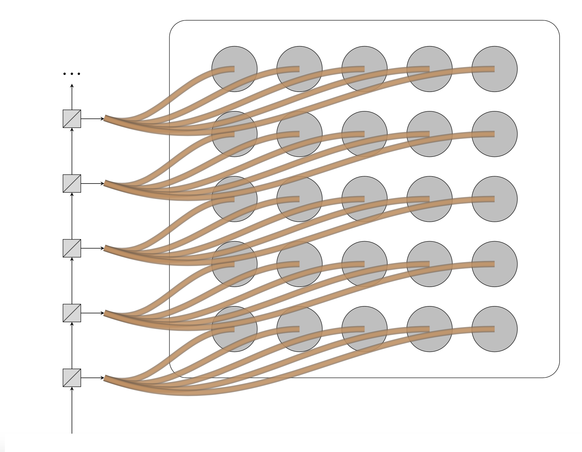
First, we focus on single-photon detection. The main reason is that number-resolved photo detection is possible using arrays of SPDs where each “pixel” receives at most one photon as in Fig. 1 (also see Nehra et al. 2017, or Migdall et al. 2003 for the time-reversed process of creating a single photon on demand). So we focus on an individual pixel here. (See Ref. Combes et al. 2017 for a modeling framework for systems with multiple inputs and Refs. Fan et al. 2010; Caneva et al. 2015; Xu and Fan 2015 for non-linear S-matrix treatments of few-photon transport.)
Second, although a general state of a single photon is a function of four quantum numbers, one related to the spectral degree of freedom, two related to the two transverse spatial degrees of freedom, and one related to the polarization or helicity degree of freedom, we will restrict ourselves to the spectral (or, equivalently, the temporal) degree of freedom. That is, the input state can be defined in terms of frequency-dependent creation operators acting on the vacuum. The reason is that the other three degrees of freedom can, in principle, if not in practice, be sorted before detection. For example, if one wishes to distinguish between horizontally and vertically polarized photons, one may use a polarizing beam splitter and put two detectors behind each of the two output ports. Similarly, efficient sorting of photons by their orbital angular momentum quantum number O’Sullivan et al. 2012 and spatial mode are also possible Bouchard et al. 2018; Fontaine et al. 2019. It is easier to consider sorting as part of the pre-detection process, rather than a task for the detector itself (see footnote 11 1 To describe sorting as well within this framework, we simply write more transmission functions, e.g. for all the different input continua , each leading to their own output continuum. Even more complicatedly, we could consider multiple outputs for a given input and write . But even in this case we can focus on a particular and as we do this in this paper.). On the other hand, the spectral response of a detector cannot be eliminated; the time/frequency degree of freedom is intrinsic to the resonance-structure of the photo detecting device.
Third, we are going to assume that each pixel’s operation is passive. That is, apart from being turned on at some point, and being turned off at some later point, it operates in a time-independent manner. Thus an incoming photon will interact with a time-independent quantum system. As we will see, active filtering is not needed for perfect detection provided the photo detector has no internal losses (couplings to additional continua).
We can now describe the interaction of a single photon with an arbitrary quantum system as follows. The system may be naturally decomposed into several subsystems, each of which may have discrete and/or continuous energy eigenstates. (For example, the photon may be absorbed by a molecule or atom or quantum dot or any structure with a discrete transition that is almost resonant with the incoming photon.) The continua will in general be structured (for example, containing bands and band gaps in between) Tellinghuisen 1975; Odegard 2002; Nygaard et al. 2008, but structured continua can be equivalently described as structureless (flat) continua coupled to (fictitious) discrete states Garraway 1997a; Garraway 1997b; Dalton et al. 2001; Mazzola et al. 2008, enabling a Markovian description of the system independent of an input photon’s bandwidth. Indeed, it is well known that a non-Markovian open system can always be made Markovian by expanding the Hilbert space (the converse of the usual Stinespring dilation Stinespring 1955). And so an arbitrary quantum system may be described by a network of discrete states (some physical, some fictitious), coupled to flat continua. The latter coupling makes the time evolution irreversible. Of course, an actual detector is indeed irreversible. In particular, the amplification process (converting the microscopic input signal into a classical macroscopic output signal) is intrinsically irreversible.
What we do here is give a general description of the photon entering some network of discrete states [indicated by the black box in Fig. 2] up to and including the first coupling to a flat continuum, that is, up to and including the first irreversible step in the process. We analyzed the (irreversible) amplification step in another paper Propp and van Enk 2019 and found the fundamental limits on added noise arising from amplification are so mild that fundamental tradeoffs of a detector are in essence determined by the pre-amplification process, which is the process we analyze here.

As we will show below, this first part of the process can then be fully described in terms of a complex transmission amplitude , which is simply the probability amplitude for the frequency component of the input signal at frequency to survive the first part of the process and enter the next (amplification) process. (By then the energy will have been converted into a different type of energy, i.e., a different type of excitation, but that plays no particular role here.) It is straightforward to calculate the transmission coefficient through a network (the equations are linear!). The point here is that from we can then determine three input-independent quantities of interest to the photo detection process. (That one complex function is sufficient is due to our considering only the time/frequency degree of freedom, see again footnote 11footnotemark: 1 ).
First, gives an upper bound on the probability for the frequency component to be detected. (If there were no losses downstream, it would equal the probability of detection.) We are thus particularly interested in identifying quantum systems for which there is at least one frequency for which .
Second, an upper bound to the total detectable frequency range is then given by the spectral bandwidth, defined as
| (1) |
(The factor gives agreement with a classical Lorentzian filter; the transmission function is for a filter with damping factor and resonant frequency and we find , see Eq. (14) below.) The inverse of this quantity is also a measure of the time the photon spends in the detector. Indeed, is a lower bound on the contribution to timing jitter from integrated detection event when quasi-monochromatic photon states are detected with high efficiency (see footnote 22 2 Timing jitter for a photo detection has three contributing components van Enk 2017b. The first comes from the temporal spread of the mode onto which the measurement projects van Enk 2017a and is intrinsic to the resonance structure of the photo detector. The second comes from integrating a continuously monitored continua to form discrete detection event, which is necessary for an accurate information-theoretic characterization of photo detection and influences photo detection efficiency (see Appendix A). It is this part of the jitter that is a lower bound for; it sets the timescale for integration where monochromatic states are detected with high efficiency. The third contribution comes from input signals with long temporal wave-packets and, since it is input-dependent, will be ignored in this analysis since here we assume no priors about the single photon input.).
Third, we can also define a delay (latency) using the polar decomposition of
| (2) |
and using the standard definition of group delay as
| (3) |
We can see how this directly relates to an experimentally-measured latency by consider an input single-photon with temporal wave packet and Fourier transform . We can then write the output single-photon state
| (4) | |||||
where the first and second terms correspond to the reflected and transmitted parts of the single-photon state, respectively (for details, see Ref. van Enk 2017a). From (4) we note that, after interacting with the network, the transmitted wave packet will have the form . For a long input pulse with central frequency , we find with the difference between the group delay defined above and the (unmeasurable) phase delay.
The effect of the group delay on an arbitrary input photon state is to selectively delay and reshape the transmitted wave packet. Of course, if an input photon has a wide spread of frequencies, a differential group delay may increase (or decrease) the temporal spread of the wave packet. This increase (or decrease) in the arrival times of different frequencies is manifestly input-dependent and will not play a role in the input-independent temporal uncertainty or jitter. We can, however, define an additional quantity characterizing the input-independent group delay-induced dispersion
| (5) |
whose definition agrees with our physical intuition that a constant group delay over the transmission window will not contribute to dispersion, nor will frequencies that are not transmitted regardless of how large may be. We find that, for a flat transmission function that is unity over some spectral range and zero everywhere else and a monotonic group delay , (5) gives the difference in group delay between the minimum and maximumly transmitted frequencies: . This is clearly the maximum dispersion possible for any input to this system.
Finding key conditions that change the transmission function and frequency-dependent group delay are important for the design of coupled-resonator optical waveguide (CROW) networks Yariv et al. 1999 for delay-lines Poon et al. 2004 and spectral filtering Madsen 2000, where the transmission efficiency, frequency-dependent group delay, and spectral bandwidth will all affect performance. These are the three quantities we focus on in the rest of the paper. We’ll start with the simplest quantum network to illustrate how we calculate and how our three quantities of interest behave. After that we’ll tackle more complicated networks.
Critically, knowing for a specific photo detector also allows one to construct the positive-operator valued measure (POVM), from which all standard figures of merit can be obtained van Enk 2017b. The POVM element corresponding to a click after the photo detector has been left on for a very long time (in particular, long compared to the bandwidth ; see Appendix A for a detailed POVM construction) has the particularly simple form
| (6) |
is defined such that the probability of a photon in a state being detected is given by the Born rule . For example, any photon state where and will be detected with unit probability. (The states the photo detector can detect perfectly include both pure states [when only one is non-zero] and mixed states comprised entirely of frequencies where . ) Of course, no photon is truly monochromatic (or discretely polychromatic, but it can be effectively so if the wave-packet envelope is long compared to the inverse spectral bandwidth .
II Simple example

The simplest quantum network consists of a single two-level system with a ground state and an excited state , with the incoming photon coupling these states (Fig. 3). The two-level system is described by fermionic raising and lowering operators and (this is also the simplest model of a photo detector, see Dewitt et al. 1965). Physically, this excited state could be any discrete state of a single absorber, e.g. the p-state of an atom which then decays to a monitored flat continuum. (Indeed, single absorbers such as atoms Cirac et al. 1997; van Enk and Kimble 2000; Tey et al. 2008; Pinotsi and Imamoglu 2008; Wang et al. 2011, single molecules Wrigge et al. 2007, NV-centers Harmon and Flatte 2019, and quantum emitters Zumofen et al. 2008; Chen et al. 2011 are known to efficiently couple to and absorb single photons.)
In the Heisenberg picture, the evolution of these raising and lowering operators and will determine whether a photon makes it from one side of the network to the other. By focusing our analysis on cases where at most a single photon is in the network, we can use the equivalence between the two-level system and the simple harmonic oscillator to simplify our problem ab initio: we replace the fermionic raising and lowering operators with bosonic creation and annihilation operators and 33 3 Since both operators and their expectation values (mode amplitudes) will satisfy the same systems of equations, we omit hats throughout this paper..
We follow standard input-output theory here Gardiner and Collett 1985, separating the full evolution of both continua and into input and output modes (Fig. 2). By formally solving the Heisenberg evolution equations for the two input continuum mode annihilation operators and , we can write the effective system Hamiltonian that governs the evolution of the system operators and
where we have identified as the resonance frequency, and and as the left and right side couplings to two continua and respectively 44 4 In assuming these couplings to be frequency independent, we are invoking a modified version of the first Markov approximation. Formally, we define where is the resonance frequency of the th discrete state and is the coupling between the th discrete state and the left continuum at the discrete state frequency. This implies that, in an experiment, the decays and resonances cannot be varied independently, which is well known in the context of the Thomas-Reiche-Kuhn sum rule for electric dipole transitions Baxter 1992. In the Heisenberg picture, the time evolution of the discrete state annihilation operator is given by
| (8) |
The input mode operators and and output mode operators and are determined by discrete state evolution of the operator and the two boundary conditions
| (9) |
It is easiest to solve the equations by taking the Fourier transform. Unitarity implies the existence of a transfer matrix relating in and out fields in the spectral domain
| (10) |
where (resulting from our assumption there are no internal losses) Vogel and Welsch 2006. Defining a detuning , we can easily solve (8) in terms of the Fourier transform of the discrete state annihilation operator
| (11) |
yielding a transmission function
| (12) |
We can see from (13) that perfect transmission () occurs only when and . These are the well-known conditions of balanced mirrors and on-resonance required for perfect transmission through a Fabry-Perot cavity Siegman 1986.
We can also calculate the frequency dependent group delay from (13)
| (13) |
We see that like , the group delay is also a Lorentzian with width , and that frequencies close to resonance spend the most time in the network with a maximum group delay of on resonance. We similarly find the input-independent group delay-induced dispersion (5) to be .
We can also use to calculate a spectral bandwidth (not to be confused with the channel bandwidth discussed in van Enk 2017b)
| (14) | |||||
| (15) |
which is a measure of the number of frequencies that can be efficiently detected. For this simple case, we note that and thus . (This will not be true for a general network, as we shall see shortly.)
III Quantum Networks
We now set up the general problem of an arbitrary network of discrete states connecting two continua. The Hamiltonian is a straightforward generalization of ()
where we’ve now defined a real coherent coupling between discrete states (we define for each state). Some states may not be coupled to one (or both) continuum, in which case either or (or both) will be zero.
We can similarly generalize the operator evolution in (8) for an arbitrary network; moving to the spectral domain, we write the spectral dependence of the discrete state operators
| (17) |
Similarly to (II), we can write boundary conditions for the two continua with an arbitrary network
| (18) |
Now going from (III) to the transfer matrix (10) involves solving systems of coupled first-order differential equations 55 5 Luckily, there is some redundancy. Once one has solved for one in terms of the input and output fields, one can permute the labels to generate the remaining solutions.. This complication occurs because each discrete state amplitude depends on every other amplitude 66 6 One alternative approach for a general network is to take the weak-coupling limit () and truncate the solutions after some power in , making (20) the th order approximate solution with higher order corrections. However, this method fails if even a single discrete state decouples from both continua.. One can also use numerical techniques to diagonalize the systems of equations and find the transmission function numerically Datta 2005. But this rapidly gets harder with large systems, and masks the analytic conditions for perfect transmission we are interested in identifying. Here, we will instead identify large classes of systems that can be solved exactly with arbitrary couplings, decays, and resonant frequencies.
Parallel: each discrete state is directly coupled to both continua ( and ) but not to each other. Thus there are multiple parallel paths to the same final state and hence we’ll get interference. Physical photo detection platforms described by parallel networks include (i) single atoms with multiple p-states that then decay directly to a continuum (similarly for trapped ions/atoms due to Stark and Zeeman effects, see Ref. Higginbottom et al. 2016 for this in generating single photons), (ii) quantum dots Livache et al. 2019, (iii) structured continua with multiple pseudomodes Hughes et al. 2018.
Series: each of the two continua are coupled to their own discrete state, which are in turn coherently coupled by a chain of intermediate single discrete states. There is just one path from the input continuum to the output continuum. This model describes (i) an atom in a p-state that first decays to a d-state or metastable s-state before decaying to a flat continuum (and analogously for a molecule Young et al. 2018), (ii) coherently coupled frequency filtering in front of a photo detecting platform (for instance, using an antireflective coating Rosfjord et al. 2006 or optical cavities Dilley et al. 2012), (iii) atomic chains coupled through their p-states (which could be mediated by, for example, a fiber mode Song et al. 2018).
Hybrid: a combination of the above cases. For example, two parallel paths of three steps each or, more generally, layered structured continua (a photon must pass through one before the other). A physical system that can be modeled with a hybrid network is a photosynthetic light-harvesting (i.e. Fenna–Matthews–Olson) complex with multiple paths for coherent transport Scholes et al. 2017; Valleau et al. 2017; Chan et al. 2018.
In all cases, we will solve the systems of equations for directly and make use of the identities and when we calculate the transmission efficiency, spectral bandwidth, and group delay.
III.1 Parallel Networks

We now consider a parallel quantum network where each discrete state is directly coupled to both continua (Fig. 4). If the discrete states are directly coupled to each other, it is helpful to first diagonalize the system in the basis where they are decoupled. We then consider the new modes to be the discrete states a photon can occupy, each with a new resonance frequency and two decay rates to the two continua. (In the strong coupling limit, Rabi splitting comes into effect and these dressed states are the more physical description anyways Steck 2018.) This decoupled manifold of discrete states, each decaying at a rate to the input continuum and a rate to the output continuum (Fig. 4), is the next simplest case to analyze, and provides a simple model of a photo detector with a simple band structure.
We find the frequency dependence of the discrete state operators
| (19) | |||||
A salient feature of Eq. 19 is the decay terms produce purely virtual coupling between discrete states coupled to the same continua. These cannot be thought of as coupling mediated by continua, as the continua are flat (Markovian) and perfectly dissipative, and is instead a purely information-theoretic phenomeona 77 7 We’ve included the assumption of a single input photon in our theory ab initio. Thus, discrete state expectation values must be correlated, manifesting as the purely virtual coupling in Eq. 19. If we relax the assumption of a single input photon, we find that these correlations still manifest in the portion of the POVM that projects onto a single photon Hilbert space, that is, the part that is relevant for single photon detection! (See Ref. van Enk 2017a for details on constructing POVMs that include general Fock states of photons.).
We use (10) to find by considering an input on only one side of the network (thus setting the expectation value of the other input field operator to zero). This yields an expression (or ), from which we reconstruct . We analytically find the general form of
| (20) |
where is a polynomial of order in the detunings . (We trivially find .) For , we can see that is symmetric (anti-symmetric) between and
| (21) |
This (anti-)symmetry is also present in higher- coefficients. From (20) we can determine a key feature of parallel quantum networks: if some subset of the discrete states have balanced decay rates such that , for large spacings between discrete states compared to the other decay rates , we find ; input monochromatic photons with frequencies on resonance with those discrete states are transmitted perfectly through the network 88 8 For , the requirement for large spacing such that is less stringent, we only need it much larger than difference in decay rates ..
In general, finding the specific form of is a numerical task, and we will focus on a simpler case where we can utilize another salient feature of parallel networks: the purely virtual coupling present in (19). Before we consider a network that is uniformly coupled (all decays are the same), we can consider a network with couplings that are inhomogeneous but uniformly unbalanced such that . We can then write (19) in a simplified form


| (22) | |||||
so that we observe strong correlations between discrete state amplitudes
| (23) |
For non-degenerate states, Eq. 23 means that a photon that is resonant with one state will only excite that state. (For infinitely-narrow discrete states, these correlations are satisfied trivially of course; is only non-zero at .) Eq. 23 also indicates that the relative phase of discrete state amplitudes is frequency dependent; when , there is a relative phase of between and . (Outside of photo detection, this purely virtual coupling provides a possible alternative explanation for the destructive interference present in atoms along a fiber Asenjo-Garcia et al. 2017; Qi et al. 2016 and multi-mode Fabry-Perot cavities Lopez-Dieguez et al. 2017.) We can see destructive interference directly from the form of the reflection coefficient
| (24) |
from which we can determine and the other quantities of interest.
We can further specialize to the case of homogenous coupling where and . This case is of interest for several reasons: most generally, this assumption directly follows from the first Markov approximation if the spacing between discrete states is small compared to the decays. It also simplifies the form of the correlations between discrete states 99 9 We now can perform a small sanity check. Considering the two continuum fields together, we define total input and output flux operators and . Solving for the total outputs directly from (III), we find . We can immediately see that ; photon flux is preserved through the system at every frequency, as it must be since there are no side channels present., as well as the form of the reflection coefficient
| (25) |
Perfect transmission.— From (24) and (25) we can see that in both cases there are frequencies of maximum transmission corresponding to each resonant frequency with transmission probability and , respectively. We also see frequencies of destructive interference corresponding to the solutions of (Fig. 5) determined solely by the decays and resonances (and notably not by ). We similarly observe for the case of a network with homogenous decay rates frequencies of destructive interference corresponding to the solutions of (Fig. 6(a)). One might think that, in principle, a resonant frequency could coincide with a frequency of perfect reflection when , in which they can annihilate. However, this only occurs when two discrete states are energetically degenerate, and since they couple to the same D continuum, this is forbidden by unitarity; as we decrease the spacing between states, we see a resonant frequency and a frequency of destructive interference annihilate as a discrete state is forced to decouple from the system as the degeneracy becomes exact.
In general, the condition for perfect transmission through a parallel network is that all the couplings be balanced ( or in the inhomogeneous uniformly unbalanced case, ). As we saw in the case for a completely arbitrary parallel network, we see that perfect transmission at some discrete state frequency not only requires balanced coupling , but also that all the other discrete states either be far away in frequency compared to the their decay rates (), or also be balanced (), or a mix of the two.
Spectral Bandwidth.— Once we have the reflection coefficient, we can calculate the three quantities of interest. For all three cases we’ve discussed, we find that the spectral bandwidth is purely additive and is completely independent of the spacing between discrete states 1010 10 The uncertainty in frequency, as defined in van Enk 2017b and calculated entropically from the spectral POVM van Enk 2017a, is in this case directly proportional to the bandwidth (and hence also independent of discrete state spacing)..
Group Delay.— We note that, unlike the simple model, the sharp peaks in the group delay (Fig. 6(b)) correspond to frequencies of destructive interference and are greatest for the outermost frequencies of destructive interference despite all the frequencies of note in (Fig. 6(a)) being completely destructive or constructive. We also observe that the relationship between the three quantities of interest discussed for the simple model is not present: here for each resonant frequency. We find that the phase of increases by with each resonant frequency (6(c)). This provides a novel application for single-photon interferometry for resolving tightly-structured resonance structures and explains why, whereas the spectral bandwidth is independent of discrete state spacing, the group delay increases with close spacing; the same change in phase is occurring in a smaller spectral range so the magnitude of the group delay increases.
III.2 Series Networks


In general, we cannot diagonalize a completely arbitrary network in terms of a single set of parallel states; there may be a causal relationship embedded in the network structure; for example, for an atom in an s-state coupled via a photon to one or many p-states which subsequently decay to multiple d-states, we would have to diagonalize the p-states and d-states separately. A class of such systems are series quantum networks (Fig. 7), where only one state is coupled to each continuum, with the other states forming a chain between the two outer ones (, , and for ). This provides a natural (and especially simple) model for energy transport and repeated spectral filtering (a series of Fabry-Perot cavities). Furthermore, we can analytically determine the transmission function for arbitrary series networks, as we will now proceed to do.


Since each state is only coupled to the two adjacent states, the system of equations of the form of (17) describing evolution of the system is solvable in a stepladder-type approach. Setting the expectation value of the second input continuum to zero, we solve for the th state in terms of the th. As we step up the ladder, we arrive at an expression for the reflection coefficient with the form of a generalized continued fraction
| (26) |
(we have dropped the subscripts on and ). This equation looks difficult to analyze, but can be simplified using the Wallis-Euler recursion relations for continued fractions. We define two function and given by the following recurrence relations
| (27) |
with coefficients and given in Fig. 8. The reflection coefficient is then given for discrete states. (For , the functions and have no clear physical meaning.) From this, we easily solve for conditions where (perfect transmission).

Perfect transmission.— We begin by considering the unphysical but illuminating case of an infinite series of identical discrete states ( and ) analytically. We find that the limit only converges on-resonance for the special “critical” case
| (28) |
Furthermore, the limit only converges to zero on resonance (perfect transmission) when we also have . This first condition corresponds to a series of discrete states coupled through their decays (e.g. Fabry-Perot cavities coupled through their evanescent fields), and the second condition corresponds to the same requirement of balanced decays we saw for parallel quantum networks.
While infinite series networks of discrete states are not realistic, these two conditions play different but important roles in all finite series networks where the discrete states are identical (though introducing relative detuning will change the critical values of and , as we will see). That there are two conditions can be explained thus; since is in general complex, the condition gives two constraint equations on the real and imaginary parts of . When is even [odd], the real part is an order [] polynomial in the detunings , while the imaginary part is order []. In general, this means there are conditions for a minimum of frequencies of perfect transmission and we may find frequencies of perfect transmission only if the lower-order equation is satisfied trivially for all frequencies. When considering finite series networks of identical discrete states, these same two conditions appear in the constraint equations for perfect transmission 1111 11 For , the lower order equation is just the requirement that and the higher order equation just requires (on-resonance). For , the lower order equation is and the higher order equation is . The lower order equation is only frequency independent when and . When the discrete states are degenerate, we find that is the requirement for perfect transmission at one () or two () frequencies..
We now explore in detail the effects of these two conditions on series networks of identical discrete states with uniform coupling; first, consider fixing the coupling to be critical (). For odd , we find that when the decays are balanced (), this ensures frequencies of perfect transmission (Fig. 9(a)) with the resonance frequency at a local maxima of unity, and when the decays are unbalanced (), frequencies of perfect transmission (Fig. 9(b)) with the resonant frequency at a local minima. For even , letting always results in frequencies of perfect transmission (Fig. 9(c)) with the on-resonant frequency at a local maxima. Here, having balanced decays broadens the the on-resonance maxima (Fig. 9(d)), which will be desirable for detection of non-monochromatic photons (wave packets).
Now we instead consider fixing the decays to be balanced () and observe a switch in the on-resonance behavior; whereas above we had found for even the critical coupling condition was sufficient for on-resonance transmission to be at a local maxima, we now find that, for odd that the balanced decay condition results in peaks of unity transmission (Fig. 10(a)) with on-resonance transmission is at a local maxima. Here three peaks become degenerate to give frequencies of perfect transmission when (Fig. 10(b)). (This inequality rapidly becomes exact [] with increasing .) Similarly, we find that for even , the behavior of depends strongly on the coupling, flipping between frequencies of perfect transmission with on-resonance transmission at a local minima for (Fig. 10(c)) and frequencies of perfect transmission with on-resonance transmission at a non-unity local maxima for (Fig. 10(d)).
For both even and odd , the width is increasingly determined by with increasing , with the half-width asymptotically approaching . In the large- limit, we observe that the transmission function is asymptotically bounded between a circle and a square when both conditions for perfect transmission are met (Fig. 11). We also observe that increasing past while maintaining induces Rabi splitting, with the or frequencies of perfect transmission spreading outwards (for odd and even , respectively). For the special case of , the presence of a second coupled discrete state resulting in a splitting and shift of the resonant frequency is in agreement with the effect seen in Ref. Rosfjord et al. 2006 for an antireflective coating; perfect transmission is still possible provided but the frequency that is perfectly transmitted is split in to two.
In the high- limit, we start seeing a frequency-comb structure emerge (Fig. 12), with dips that approach perfect reflection. This is because in the strong-coupling limit, the causal ordering of the discrete states asymptotically disappears: the system becomes approximately diagonalizable as parallel modes with purely virtual coupling and the frequencies of perfect reflection from (24) manifest.
We now consider the effects of introducing relative detunings between discrete states as, generally, a quantum network will not be comprised of identical states. Still there are sufficient degrees of freedom in (26) such that, by tuning the parameters, perfect transmission at some frequencies is always possible. This is even true when (for ): considering only two discrete states in series, we find that perfect transmission occurs at a frequency when (Fig. 13). For two detuned discrete states in series with balanced decays (), perfect transmission is impossible as the critical value of is infinite; the transmission efficiency asymptotically becomes perfect in the strong-coupling limit. However, this a special case and is not true for larger numbers () discrete states. Critically, given a series network of discrete states with arbitrary relative detunings, we can always find at least one set of parameters (couplings and decay rates) such that frequencies are perfectly transmitted.

Spectral Bandwidth.— Once we have the form of the transmission function, we can calculate the spectral bandwidth for these systems. The spectral bandwidth decreases with additional discrete states and is strictly bounded above by the single discrete state bandwidth . For discrete states without detuning, equality is reached in the strong-coupling limit of but independently of whether (Fig. 14). Introducing detuning between discrete states lowers the bandwidth, but equality with the upper limit still occurs for sufficiently strong coupling (Fig. 15); the strong coupling is able to better mask the discrepancy between discrete state frequencies as the dressed states become the more physical description and as the system more strongly resembles a parallel network. (In this limit, each dressed state is coupled to the continua at reduced decays so that the total bandwidth is still bounded by with and the two original decay rates for the series network.)
Group Delay.— Lastly, we consider the group-delay for series networks, which increases with both and but for different reasons. As increases, the peaks of the transmission function sharpen so that the phase changes more rapidly. This results in an increased group delay (Fig. 16(a)-d). As increase, we observe (as we did for parallel networks) that the peaks in the group delay are not of uniform magnitude, even when the transmission function itself is rather flat (Fig. 17(a)). Instead, the frequencies of maximum delay are those closest to (Fig. 17(c)) increase the most with . This is because the oscillations in the transmission function are most dense here, resulting in a rapid change in transmission function phase and thus a larger group delay. On the contrary, the group delay is relatively flat in the center of the transmission window (Fig. 17(c)) so that a spectrally-narrow (compared to ) input photon pulse will not be significantly dispersed. (That is, the maximum dispersion-induced jitter from (5) will be very small.)

We can also consider the effect of detunings on the frequency-dependent group delay. We observe the group delay can be negative for series networks with detuning (Fig. 17(d)), with an asymmetric structure that depends on the ordering of the detunings (except in the strongly coupled limit). Again, the magnitude of the group delay depends on the spacing of discrete states, increasing when the resonant frequencies are closely spaced.


III.3 Hybrid Networks

We now begin to approach the case of a general two-sided quantum network. The fully general problem is intractable analytically, but luckily there are several simplifications we can make that correspond to the network representing realistic photo detecting systems. To illustrate, consider the case of two parallel networks in series: each discrete state connected to each discrete state in the other manifold (but not necessarily at the same rate) with each of the two manifolds of purely virtually coupled discrete states coupled to their own continuum. One could imagine generating different networks from this one by removing a coupling between discrete states, permuting which discrete states are disconnected, removing an additional coupling, permuting, and so on. However, this is unphysical: two discrete states in parallel cannot be prevented from coupling to the same discrete state except by selection rules. But the discrete states are also coupled to the same continuum (which has been already made D in effect), so they must satisfy the same selection rules. The same argument applies in reverse: no discrete state within a manifold can individually stop being coupled to a continuum without the rest of the discrete states doing so as well. And we can similarly apply it to manifolds embedded in a larger network away from a continuum: the requirement that all states satisfy the same selection rules is strong. This means we can ignore partially connected networks. It also gives us a helpful way to organize discrete states: into manifolds of discrete states (which are purely virtually coupled to each other after diagonalization) that are all coupled to the same set of discrete or continuum states.
We can now focus on a very large class of quantum networks, hybrid systems consisting of manifolds in series (Fig. 18). It will be helpful to denote couplings between discrete states and or manifolds and as , and denote decay rates and discrete states within a manifold with a superscript (, , and , with for and for , where is the number of manifolds). This allows us to rewrite the general equation (17) in a more explicit form
| (29) | |||||
where the superscripts denote labels of manifolds and we’ve implicitly defined . We denote the number of discrete states in each manifold such that . In general (29) is still only numerically solvable but we can now note two cases that yield analytic solutions.


The first is the case of critical coupling between members of each adjacent manifold and, additionally, uniformly unbalanced decays: we first define an effective decay rate for internal couplings within the system so that (effectively specializing to the critical coupling case for series networks), and then consider the special case of (inhomogeneous decays that are uniformly unbalanced within each manifold). This leads to a reflection coefficient of the form
where we have defined a new function . (The appearance of a lone at the end of () is due to the final purely virtual coupling to the output continuum, since we’ve absorbed the rest of the decay rate into the function .) This function encodes the zeroes and singularities we found for parallel networks, which previously gave rise to frequencies of constructive interference and completely destructive interference.
While () is tractable, it is of limited applicability to real systems. More relevant is the second solvable case of homogenous coupling and decays within manifolds: , , and . This leads to a reflection coefficient of the form
where again we have defined a new function . This provides a nice model for multi-mode systems in series (for instance, a linear network of identical multimode optical cavities).
We see in both () and () a combination of the structures we observed in (24) and (25) for parallel networks and (26) for series networks: correlations in amplitudes between discrete states within a given manifold manifest via a function or with poles and zeroes (potentially perfectly transmitted and reflected frequencies, depending on the hybrid network’s resonance structure and couplings), and causal ordering of the manifolds manifests in a continued fraction structure. This latter property makes them easily analyzable using the Wallis-Euler recurrence relations, allowing us to find and from there and the other quantities of interest.
Perfect transmission.— Focusing on the case of homogenous coupling, we can use the same trick of examining the convergence of an infinite series of identical manifolds around one of resonant frequencies to find the two critical conditions as we did for series networks, which again are and . We also observe that the form of for hybrid systems exhibits a combination of features of series and parallel networks (Fig. 19(a) and 20(a)). This results in layers of structure, with the small dips and peaks corresponding to intra-manifold structure layered on top of the larger dips and peaks of the inter-manifold structure.
When at least one discrete state in each manifold have the same resonance, letting and ensures perfect transmission at frequencies. For a general hybrid network, the number of peaks of unity (perfect transmission) of are bounded above by , with the number of manifolds each with discrete states. Here the latter equality is reached for networks that are either completely in parallel or completely in series, with critical parameters in either case 1212 12 The bound is somewhat stronger for critically coupled networks, with the number of perfectly transmitted frequencies bounded by instead. This is due to the on-resonance broadening that occurs for critically coupled systems, which prevents the splitting of one peak to two when the number of manifolds is even..
Spectral Bandwidth.— For hybrid networks where the first and last manifold have the same number of discrete states , the spectral bandwidth is bounded above by the parallel network bandwidth for that number of discrete states with equality reached in the strong coupling limit. (When the first and last manifold have different number of discrete states , the bandwidth is bounded above by for a homogeneously decaying network with a network-dependent number that is always less than .)
Group Delay.— We observe the same structural properties of the group delay (Fig. 19(b)) as we did for other networks; the frequencies with the largest delays are those where oscillations in the transmission function are most dense. We find that networks with non-identical manifolds can give rise to group delays that are not strictly positive (Fig. 20(b)).


IV Other Networks
IV.1 General Two-Sided Networks
We now begin to extrapolate from the above analyses to a larger class of two-sided networks. Both the series networks and hybrid networks we’ve discussed have the key property of asymptotic irrelevance of the causal ordering of discrete states in the strong coupling limit. This means that the asymptotically strong-coupling behavior of these networks is entirely determined by the properties of fully parallel networks (20), and we can make several statements that will apply to any network that has the same behavior (that is, a network that resembles (20) in the strong coupling limit). From the structure of (20) alone, we can bound the total number of peaks and troughs of ; we find there are at most peaks and troughs in the strong coupling limit and since the number of maxima never decreases with increasing , we can extrapolate these bounds to weakly coupled systems as well. In transitioning from peaks or constructive interference to peaks of perfect transmission, we observe a pair-wise merging of peaks (with one extra peak leftover when is odd). We also find that the number of dips of zero transmission (perfect reflection) is at most where the latter equality is only reached for a completely parallel network or in the strong coupling limit.
We suspect that the above argument for upper bounds applies more generally than just to the specific networks consisting of manifolds in series; that is, there is a large class of networks that reduce to a parallel description in the strong coupling limit 1313 13 It’s worth reiterating here that all networks reduce to (20) in the very-weak coupling limit . However, we cannot generalize from the above analysis to a fully arbitrary two-sided network as there also are networks with different topologies. For instance, we can consider networks with loops of discrete states that exist outside the main chain of manifolds that connect the two continua. Since it is not necessary for a photon to pass through the loop of discrete states to make it through the network, these networks behave differently in the strong coupling limit. We can make a further distinction between disconnected loops (dead-ends where photons have to back track) and connected loops (chains of manifolds that provide an alternate route to the output continua). It is possible that connected loops behave more like the loop-free networks discussed above in the strong-coupling limit, but with their specific loop-structure encoded in in unexpected ways.
IV.2 Additional Continua

We have thus far only considered quantum networks with two continnua, and have shown that perfect transmission through a general network structure is possible. We will briefly analyze more general multi-port quantum networks (Fig. 22) to illustrate how they lead to inefficiencies and dark counts.
Introducing a third continuum coupled to our network of discrete states at rates , we rewrite (17) in the form
| (32) |
where we have introduced a new input field annihilation operator for the additional continuum (satisfying the canonical commutation relations), satisfying the same form of input-output relations as in (III)
| (33) |
When there are side channels and all decay rates in the system are homogenous (, , and ), it is impossible to achieve perfect transmission at any input frequency without adding additional excitations (active filtering). To see this, consider taking expectation values and imposing over all frequencies. Flux conservation requires that, for a perfectly transmitted frequency , we also have . From (33), we see the only way to achieve this is for but from (III), we see that this results in and —the frequency is instead perfectly reflected by the system.
It is still possible that side channels with inhomogeneous coupling could yield a system that perfectly transmit some light at a frequency satisfying both conditions and . After all, the with resonant frequencies above and below generically differ in phase by and could in principle cancel out. However, this would require incredible fine-tuning of the system. For a uniformly inhomogeneous parallel network such as (24) with a side channel, we can easily see that this approach fails even in the low-loss limit near resonance (where it would be most likely to succeed): we find . In general, output channels outside your control lead to loss.
Similarly, we can determine from (32) and (33) that, in general, input channels outside your control lead to extra dark counts; photons that are in initially populated side channel can end up in the monitored continuum. If the side channel is at a finite temperature, there will be thermal photons that could populate the system. The probability of this vanishes for , but will generally be non-negligible for high-temperature systems. The specific contribution depends on the specific form of the full transfer matrix, which now will include a function that governs the probability of thermal excitations in the side channel to end up in the monitored continuum.
Of course, the internal mode may be occupied by thermal excitations as well, but the contribution to dark counts by these will depend strongly on the amplification mechanism. Furthermore, if only frequencies such that are amplified, we find that thermal excitations do not contribute at all to dark counts as they always leak out of the system, ending up in the continuum mode populated by reflected input photons.
V Conclusions
We have studied the behavior of coherent quantum networks and have found that they provide a diverse structure of transmission functions for modeling the first stage of single photon detectors (transmission of a single excitation from the input continuum, through the system, to a monitored output continuum). Inefficiencies and dark counts can be modeled through the incorporation of additional continua (side channels). While we do not find fundamental limits to transmission efficiency, spectral bandwidth, or frequency-dependent group delay across all the studied networks (series, parallel, and hybrid), we do find that some networks are better suited to certain applications than others, as we will now discuss.
Perfect Transmission.— Often the most important metric for a photo detector is photo detection efficiency, which for a quantum network is tantamount to ensuring is achieved for some frequency or frequencies . The main conclusions of this paper are as follows:
- (i)
Ensuring the decay rates to the input and output continua are balanced () guarantees perfect transmission for at least one frequency in almost all quantum networks without loops, side channels, and detunings [including all not covered by (ii)].
- (ii)
Ensuring the couplings between manifolds are uniform and critical () guarantees perfect transmission for at least one frequency in almost all quantum networks without loops, side channels, and detunings [including all not covered by (i)].
- (iii)
For an arbitrarily detuned quantum network without loops and side channels, we are always able to find conditions for the couplings and decay rates such that perfect transmission occurs for at least one frequency.
That finding conditions such that perfect transmission is always possible indicates that perfect photo detection is possible in a wide variety of physical systems.
If one additionally wants a broadened transmission spectrum at a particular perfectly transmitted frequency—so that a broad range of frequencies is detected almost perfectly—we similarly find a variety of ways to accomplish it. One way is to use a parallel network distributed over a small range of states. However, this will result in a number of dark states which will not be detected at all (spectral hole-burning). Instead, it is better to use a series network that meets both the critical coupling and balanced decay conditions, resulting in a maximally broadened on resonance transmission function as seen in Fig. 11.
Spectral Bandwidth.— We do not find fundamental limits to the minimum or maximum bandwidth of a network (or, conversely, to the interaction time between a network and incident light ), but that it is generally proportional to the decay rates to both the input and monitored continua (, here assumed to be homogenous across states). We also find that some network structures are more suited to high-bandwidth applications than others; for networks with equivalent decay rates, we generally find that . For a series network, equality with the upper limit of is reached only in the strong-coupling limit, and the lower limit () corresponds to a completely de-coupled or infinitely-detuned network (so that a photon can never pass through). For a parallel network, the bandwidth is always given regardless of detuning, so the lower limit simply corresponds to a single discrete state (reproducing the simple model). Unlike both series and hybrid networks where the spectral bandwidth decreases with detuning, the spectral bandwidth of a parallel network is independent of detuning. This makes parallel networks the better candidate for implementation of broadband single photon detection where the frequencies that need to be detected are distinct (so that spectral hole-burning is a non-issue).
Considering hybrid networks, we find that their bandwidths are bounded above and below by parallel and series networks, respectively; given a series network with the same coupling strengths and manifold-number, and a parralel network with the same manifold resonance structure and decay rates, the bandwidth of a Hybrid network is bounded . The upper limit for a hybrid network is approached only in the limit of strong coupling, and the lower limit is approached when there is only a single discrete state in each manifold.
Group Delay.— The maximum magnitude of frequency-dependent group delay increases with both the couplings between discrete states and the density of oscillations in the transmission function . In particular, the bounded-box structure of a uniformly coupled series networks yields large delays near . We observe that a negative group delay may occur for series networks with relative detuning between the discrete states. (For more on negative group delay, see Ref. Solli et al. 2002.) For general networks, the group delay can vary immensely over the range of frequencies where is non-negligible, with the effect being strongest for hybrid networks (where the resonance structures can be most dense). This means we can expect dispersion effects to be substantial in many photo detection platforms. For applications such as frequency discriminating delay-lines, we may expect hybrid networks to be the best performing candidate as they allow for the finest control of group delay structure.
Tradeoffs.— For an arbitrary series or hybrid network with arbitrary decay rates, perfect transmission requires a particular choice of the couplings. This critical value is generically of order . However, the spectral bandwidth is maximized when . Furthermore, the magnitude and location of the maximum group delays depends strongly on the coupling (and especially so in the high- limit). So for series and hybrid networks, there is a clear tradeoff between efficient transmission and the spectral bandwidth (which saturates in the high- limit) 1414 14 Of course, this assumes a large spectral bandwidth is a desired. There is always an obvious tradeoff between the spectral bandwidth and the amount one learns about the incoming light; the more frequencies that can be detected efficiently, the less a single click tells you about the incoming light. Whether a high bandwidth or a low bandwidth is preferred will ultimately depend on the application of a SPD., with the group delay changing as well. We contrast this with the case of parallel networks where the three quantities are completely independent: perfect detection requires balanced decays (), the bandwidth can be directly scaled by scaling both decay rates together, and the frequency-dependent group delay alone depends on the detuning between discrete states, which is an independent quantity. So for photo detectors where all three quantities must be determinable independently, parallel networks form the clear contenders. The exception to this are situations where a negative group delay is required, which parallel networks never exhibit. Then the use of a hybrid or series network is unavoidable, as are their accompanying tradeoffs.
Final Remarks.— We have studied a variety of quantum networks to uncover tradeoffs and limits fundamental to single photon detection that may arise in the first step of photo detection (filtering). The spectral bandwidth is the only main quantity of interest where there appear to be fundamental limits for particular classes of networks (parallel, series, and hybrid), but even these scale with the relevant decay rates for the networks. Given the freedom to adjust coupling strengths and decay rates, arbitrary group delay, transmission efficiency, and spectral bandwidth are attainable for any network so long as they are attained individually (together there may be tradeoffs for series and hybrid networks).
We do not find fundamental limitations to dark counts and losses in this analysis: in general uncontrolled input channels lead to dark counts and uncontrolled output channels lead to loss. These can always be mitigated by cooling the system () and reducing coupling to side channels ().
Other sources of noise, such as from signal amplification (for more on this specifically, see Ref. Propp and van Enk 2019), classical parameter fluctuations, as well as the noise inherent in a non-ideal quantum measurement (as described by an arbitrary photo detection POVM) can also be included in our model to give a fully quantum description of the entire single photon detection process Propp and van Enk.
This work is supported by funding from DARPA under Contract No. W911NF-17-1-0267.
References
- Young et al. (2018) S. M. Young, M. Sarovar, and F. Léonard, Phys. Rev. A 97, 033836 (2018).
- Sunter and Berggren (2018) K. A. Sunter and K. K. Berggren, Appl. Opt 57, 4872 (2018).
- Gemmell et al. (2017) N. R. Gemmell, M. Hills, T. Bradshaw, T. Rawlings, B. Green, R. M. Heath, K. Tsimvrakidis, S. Dobrovolskiy, V. Zwiller, S. N. Dorenbos, M. Crook, and R. H. Hadfield, Supercond. Sci. Technol. 30, 11LT01 (2017).
- Dewitt et al. (1965) C. Dewitt, A. Blandin, and C. Cohen-Tannoudji, eds., Quantum Optics and Electronics (1965).
- Mandel and Wolf (1995) L. Mandel and E. Wolf, Optical Coherence and Quantum Optics, 2nd ed. (Cambridge University Press, 1995).
- Kelley and Kleiner (1964) P. L. Kelley and W. H. Kleiner, Phys. Rev. 136, A316 (1964).
- Scully and Lamb (1969) M. O. Scully and W. E. Lamb, Phys. Rev. 179, 368 (1969).
- Yurke and Denker (1984) B. Yurke and J. S. Denker, Phys. Rev. A 29, 1419 (1984).
- Ueda (1999) M. Ueda, Quantum Opt.: J. Eur. Opt. Soc. B 1, 131 (1999).
- Schuster et al. (2005) D. I. Schuster, A. Wallraff, A. Blais, L. Frunzio, R.-S. Huang, J. Majer, S. M. Girvin, Schoelkopf, and RJ, Phys. Rev. Lett. 94, 123602 (2005).
- Clerk et al. (2010) A. A. Clerk, M. H. Devoret, S. M. Girvin, F. Marquardt, and R. J. Schoelkopf, Rev. Mod. Phys. 82, 1155 (2010).
- Propp and van Enk (2019) Tz. B. Propp and S. J. van Enk, Opt. Express 27, 23454 (2019).
- Helmer et al. (2009) F. Helmer, M. Mariantoni, E. Solano, and F. Marquardt, Phys. Rev. A 79, 052115 (2009).
- Nehra et al. (2017) R. Nehra, C.-H. Chang, A. Beling, and O. Pfister, arXiv preprint arXiv:1708.09015 (2017).
- Migdall et al. (2003) A. L. Migdall, S. Castelletto, and M. J. Ware, in Quantum Information and Computation, Vol. 5105 (International Society for Optics and Photonics, 2003) pp. 294–303.
- Combes et al. (2017) J. Combes, J. Kerckhoff, and M. Sarovar, Adv. Phys: X 2, 784 (2017).
- Fan et al. (2010) S. Fan, Ş. E. Kocabaş, and J.-T. Shen, Phys. Rev. A 82, 063821 (2010).
- Caneva et al. (2015) T. Caneva, M. T. Manzoni, T. Shi, J. S. Douglas, J. I. Cirac, and D. E. Chang, New J. Phys. 17, 113001 (2015).
- Xu and Fan (2015) S. Xu and S. Fan, Phys. Rev. A 91, 043845 (2015).
- O’Sullivan et al. (2012) M. N. O’Sullivan, M. Mirhosseini, M. Malik, and R. W. Boyd, Opt. Express 20, 24444 (2012).
- Bouchard et al. (2018) F. Bouchard, N. H. Valencia, F. Brandt, R. Fickler, M. Huber, and M. Malik, Opt. Express 26, 31925 (2018).
- Fontaine et al. (2019) N. K. Fontaine, R. Ryf, H. Chen, D. T. Neilson, K. Kim, and J. Carpenter, Nat. Commun. 10, 1865 (2019).
- (23) To describe sorting as well within this framework, we simply write more transmission functions, e.g. for all the different input continua , each leading to their own output continuum. Even more complicatedly, we could consider multiple outputs for a given input and write . But even in this case we can focus on a particular and as we do this in this paper.
- Tellinghuisen (1975) J. Tellinghuisen, Phys. Rev. Lett. 34, 1137 (1975).
- Odegard (2002) G. Odegard, Compos. Sci. Technol. 62, 1869 (2002).
- Nygaard et al. (2008) N. Nygaard, R. Piil, and K. Mølmer, 78, 023617 (2008).
- Garraway (1997a) B. M. Garraway, Phys. Rev. A 55, 2290 (1997a).
- Garraway (1997b) B. M. Garraway, Phys. Rev. A 55, 4636 (1997b).
- Dalton et al. (2001) B. J. Dalton, S. M. Barnett, and B. M. Garraway, Phys. Rev. A 64, 053813 (2001).
- Mazzola et al. (2008) L. Mazzola, S. Maniscalco, J. Piilo, K. A. Suominen, and B. M. Garraway, Pseudomodes as an effective description of memory, Tech. Rep. (2008).
- Stinespring (1955) W. F. Stinespring, P. Am. Math. Soc. 6, 211 (1955).
- Gardiner and Collett (1985) C. W. Gardiner and M. J. Collett, Phys. Rev. A 31, 3761 (1985).
- (33) Timing jitter for a photo detection has three contributing components van Enk 2017b. The first comes from the temporal spread of the mode onto which the measurement projects van Enk 2017a and is intrinsic to the resonance structure of the photo detector. The second comes from integrating a continuously monitored continua to form discrete detection event, which is necessary for an accurate information-theoretic characterization of photo detection and influences photo detection efficiency (see Appendix A). It is this part of the jitter that is a lower bound for; it sets the timescale for integration where monochromatic states are detected with high efficiency. The third contribution comes from input signals with long temporal wave-packets and, since it is input-dependent, will be ignored in this analysis since here we assume no priors about the single photon input.
- van Enk (2017a) S. J. van Enk, Phys. Rev. A 96, 033834 (2017a).
- Yariv et al. (1999) A. Yariv, Y. Xu, R. K. Lee, and A. Scherer, Opt. Lett. 24, 711 (1999).
- Poon et al. (2004) J. K. Poon, J. Scheuer, Y. Xu, and A. Yariv, J. Opt. Soc. Am. B 21, 1665 (2004).
- Madsen (2000) C. K. Madsen, J. Light. Technol. 18, 860 (2000).
- van Enk (2017b) S. J. van Enk, J. Phys. Comm. 1, 045001 (2017b).
- Cirac et al. (1997) J. I. Cirac, P. Zoller, H. J. Kimble, and H. Mabuchi, Phys. Rev. Lett. 78, 3221 (1997).
- van Enk and Kimble (2000) S. J. van Enk and H. J. Kimble, Phys. Rev. A 61, 051802(R) (2000).
- Tey et al. (2008) M. K. Tey, Z. Chen, S. A. Aljunid, B. Chng, F. Huber, G. Maslennikov, and C. Kurtsiefer, Nat. Phys. 4, 924 (2008).
- Pinotsi and Imamoglu (2008) D. Pinotsi and A. Imamoglu, Phys. Rev. Lett. 100, 093603 (2008).
- Wang et al. (2011) Y. Wang, J. Minář, L. Sheridan, and V. Scarani, Phys. Rev. A 83, 063842 (2011).
- Wrigge et al. (2007) G. Wrigge, I. Gerhardt, J. Hwang, G. Zumofen, and V. Sandoghdar, Nat. Phys. 4, 60 (2007).
- Harmon and Flatte (2019) N. J. Harmon and M. E. Flatte, arXiv preprint arXiv:1906.01800 (2019).
- Zumofen et al. (2008) G. Zumofen, N. M. Mojarad, V. Sandoghdar, and M. Agio, Phys. Rev. Lett. 101, 180404 (2008).
- Chen et al. (2011) Y. Chen, M. Wubs, J. Mørk, and A. F. Koenderink, New J. Phys. 13, 103010 (2011).
- (48) Since both operators and their expectation values (mode amplitudes) will satisfy the same systems of equations, we omit hats throughout this paper.
- (49) In assuming these couplings to be frequency independent, we are invoking a modified version of the first Markov approximation. Formally, we define where is the resonance frequency of the th discrete state and is the coupling between the th discrete state and the left continuum at the discrete state frequency. This implies that, in an experiment, the decays and resonances cannot be varied independently, which is well known in the context of the Thomas-Reiche-Kuhn sum rule for electric dipole transitions Baxter 1992.
- Vogel and Welsch (2006) W. Vogel and D.-G. Welsch, Quantum Optics, 3rd ed. (Wiley-VCH, 2006).
- Siegman (1986) A. E. Siegman, Lasers (University Science Books, 1986).
- (52) Luckily, there is some redundancy. Once one has solved for one in terms of the input and output fields, one can permute the labels to generate the remaining solutions.
- (53) One alternative approach for a general network is to take the weak-coupling limit () and truncate the solutions after some power in , making (20) the th order approximate solution with higher order corrections. However, this method fails if even a single discrete state decouples from both continua.
- Datta (2005) S. Datta, Quantum Transport: Atom to Transistor, 2nd ed. (Cambridge University Press, 2005).
- Higginbottom et al. (2016) D. B. Higginbottom, L. Slodička, G. Araneda, L. Lachman, R. Filip, M. Hennrich, and R. Blatt, New J. Phys. 18, 093038 (2016).
- Livache et al. (2019) C. Livache, B. Martinez, N. Goubet, C. Gréboval, J. Qu, A. Chu, S. Royer, S. Ithurria, M. G. Silly, B. Dubertret, and E. Lhuillier, Nat. Commun. 10, 2125 (2019).
- Hughes et al. (2018) S. Hughes, M. Richter, and A. Knorr, Opt. Lett. 43, 1834 (2018).
- Rosfjord et al. (2006) K. M. Rosfjord, J. K. W. Yang, E. A. Dauler, A. J. Kerman, V. Anant, B. M. Voronov, G. N. Goltsman, and K. K. Berggren, Opt. Express 14, 527 (2006).
- Dilley et al. (2012) J. Dilley, P. Nisbet-Jones, B. W. Shore, and A. Kuhn, Phys. Rev. A 85, 023834 (2012).
- Song et al. (2018) G.-Z. Song, E. Munro, W. Nie, L.-C. Kwek, F.-G. Deng, and G.-L. Long, Phys. Rev. A 98, 023814 (2018).
- Scholes et al. (2017) G. D. Scholes, G. R. Fleming, L. X. Chen, A. Aspuru-Guzik, A. Buchleitner, D. F. Coker, G. S. Engel, R. van Grondelle, A. Ishizaki, D. M. Jonas, J. S. Lundeen, J. K. McCusker, S. Mukamel, J. P. Ogilvie, A. Olaya-Castro, M. A. Ratner, F. C. Spano, K. B. Whaley, and X. Zhu, Nature 543, 647 (2017).
- Valleau et al. (2017) S. Valleau, R. A. Studer, F. Häse, C. Kreisbeck, R. G. Saer, R. E. Blankenship, E. I. Shakhnovich, and A. Aspuru-Guzik, ACS Cent. Sci 3, 1086 (2017).
- Chan et al. (2018) H. C. H. Chan, O. E. Gamel, G. R. Fleming, and K. B. Whaley, J. Phys. B 51, 054002 (2018).
- Steck (2018) D. A. Steck, Quantum and Atom Optics, (Available online at http://steck.us/teaching, revision 0.12.3, 25 October 2018).
- (65) We’ve included the assumption of a single input photon in our theory ab initio. Thus, discrete state expectation values must be correlated, manifesting as the purely virtual coupling in Eq. 19. If we relax the assumption of a single input photon, we find that these correlations still manifest in the portion of the POVM that projects onto a single photon Hilbert space, that is, the part that is relevant for single photon detection! (See Ref. van Enk 2017a for details on constructing POVMs that include general Fock states of photons.).
- (66) For , the requirement for large spacing such that is less stringent, we only need it much larger than difference in decay rates .
- Asenjo-Garcia et al. (2017) A. Asenjo-Garcia, J. D. Hood, D. E. Chang, and H. J. Kimble, Phys. Rev. A 95, 033818 (2017).
- Qi et al. (2016) X. Qi, B. Q. Baragiola, P. S. Jessen, and I. H. Deutsch, Phys. Rev. A 93, 023817 (2016).
- Lopez-Dieguez et al. (2017) Y. Lopez-Dieguez, J. Estudillo-Ayala, D. Jauregui-Vazquez, J. Sierra-Hernandez, L. Herrera-Piad, J. Cruz-Duarte, J. Hernandez-Garcia, and R. Rojas-Laguna, Optik 147, 232 (2017).
- (70) We now can perform a small sanity check. Considering the two continuum fields together, we define total input and output flux operators and . Solving for the total outputs directly from (III), we find . We can immediately see that ; photon flux is preserved through the system at every frequency, as it must be since there are no side channels present.
- (71) The uncertainty in frequency, as defined in van Enk 2017b and calculated entropically from the spectral POVM van Enk 2017a, is in this case directly proportional to the bandwidth (and hence also independent of discrete state spacing).
- (72) For , the lower order equation is just the requirement that and the higher order equation just requires (on-resonance). For , the lower order equation is and the higher order equation is . The lower order equation is only frequency independent when and . When the discrete states are degenerate, we find that is the requirement for perfect transmission at one () or two () frequencies.
- (73) The bound is somewhat stronger for critically coupled networks, with the number of perfectly transmitted frequencies bounded by instead. This is due to the on-resonance broadening that occurs for critically coupled systems, which prevents the splitting of one peak to two when the number of manifolds is even.
- (74) It’s worth reiterating here that all networks reduce to (20) in the very-weak coupling limit .
- Solli et al. (2002) D. Solli, R. Y. Chiao, and J. M. Hickmann, Phys. Rev. E 66, 056601 (2002).
- (76) Of course, this assumes a large spectral bandwidth is a desired. There is always an obvious tradeoff between the spectral bandwidth and the amount one learns about the incoming light; the more frequencies that can be detected efficiently, the less a single click tells you about the incoming light. Whether a high bandwidth or a low bandwidth is preferred will ultimately depend on the application of a SPD.
- (77) Tz. B. Propp and S. J. van Enk, in preparation .
- Baxter (1992) C. Baxter, J. Phys. B 25, L589 (1992).
- Molmer and Castin (1996) K. Molmer and Y. Castin, Quantum Semiclass. Opt.: J. Eur. Opt. Soc. B 8, 49 (1996).
Appendix A Photo detection POVM
So far in this paper, we have not discussed in detail what happens to the excitation after it ends up in the output mode , except that it gives rise to a macroscopic photo detector click. Following Ref. van Enk 2017a, we can construct the full POVM describing a photo detector from which all standard figures of merit can be obtained van Enk 2017b. Assume that we finalize the photo detection process by simply ascertaining at some time whether the excitation is indeed in and also that the amplification is ideal and lossless so that, if a photon makes it to the monitored continuum, it will be detected (this assumption is revisited in more depth in Propp and van Enk 2019). We can then define normalized filtered photon states
| (34) |
From the quantum jump method Molmer and Castin 1996; Mazzola et al. 2008, we know that a quantum jump from the last manifold of discrete states to the monitored continuum will occur in an infinitesimal time with condition probability . We can then infer the POVM element for detecting a photon at a particular time after the photo detector has been on for a time
| (35) |
(To reiterate, here refers to the time of detection, not the time evolution of the input state.) The probability of getting a click for a normalized input photon is . So the input state that will be detected with maximum probability is , yielding an infinitesimal probability of detection of . This is because this assumes that the detection events at times separated by a time correspond to different measurement outcomes which is highly idealized; any realistic photo detection outcome corresponds to detection within an integrated time-window (see again footnote 11footnotemark: 1 ).
To take a finite time-window into account, we consider a time-integrated POVM element , where a click corresponds to a detection event sometime between and . Then the time-integrated POVM element is
| (36) |
where, for , the projectors are truly monochromatic because no timing information is obtained. With the time-integrated form in (A), we can see that the conditions for perfect transmission discussed above correspond to perfect detection in the limit of as we used previously in (6). Physically, a non-infinitesimal integration time means a photon incident on the photo detector at a time has had sufficient time to propagate through the network before we end the integration at time and check whether there has been a click. This is in agreement with our observation that, for the simple model in (8), : we must at least allow enough time for an on-resonance photon to travel through the network (interact with the device) to achieve perfect detection of a monochromatic on-resonance photon. (A) is also illustrative of what the POVM element represents: the information a detector click reveals about what led up to it.
We can also use (A) to construct the POVM element for not getting a click in the finite time , which is simply , such that the full POVM forms a partition of unity for the relevant Hilbert space; that is, the Hilbert space spanned by single photon states and the vacuum. (See Ref. van Enk 2017b for inclusion of general photon Fock states in the photo detection POVM.) This POVM corresponds to a photo detector that is reset after each integration time . Similarly, one can divide up the the full detection window into time intervals without resetting the device in between so that the full POVM is . In this case, the measurement outcomes are not orthogonal van Enk 2017a; even if we know a photon is incident at a definite time we cannot predict with certainty when it will be detected.