跳到论文正文
W Papers独立论文阅读器 arXiv:1901.09912 论文正文 计算阅读时间 · 0%
引用这篇论文根据当前论文元数据生成,正式投稿前建议核对。


License: arXiv.org perpetual non-exclusive license
arXiv:1901.09912v1 [math.CA] 28 Jan 2019

Further Spectral Properties of the Weighted Finite Fourier Transform Operator and Approximation in Weighted Sobolev Spaces.

NourElHouda Bourguibaa and Ahmed Souabnia 11 1 Corresponding author: Ahmed Souabni, email: souabniahmed@yahoo.fr
This work was supported in part by the Tunisian DGRST research grants UR 13ES47.

a University of Carthage, Department of Mathematics, Faculty of Sciences of Bizerte, Tunisia.

Abstract— In this work, we first give some mathematical preliminaries concerning the generalized prolate spheroidal wave function (GPSWFs). This set of special functions have been introduced in [21] and [13] and they are defined as the infinite and countable set of the eigenfunctions of a weighted finite Fourier transform operator. Then, we show that the set of the singular values of this operator has a super-exponential decay rate. We also give some local estimates and bounds of these GPSWFs. As an application of the spectral properties of the GPSWFs and their associated eigenvalues, we give their quality of approximation in a weighted Sobolev space.Finally, we provide the reader with some numerical examples that illustrate the different results of this work.

1 Introduction

We first recall that for c>0c>0, the classical prolate spheroidal wave functions (PSWFs) were first discovered and studied by D. Slepian and his co-authors, see [18, 19]. These PSWFs are defined as the solutions of the following energy maximization problem :

 Find ​g=arg⁡maxf∈Bc⁡∫−11|f⁡(t)|2​𝑑t∫ℝ|f⁡(t)|2​𝑑t\mbox{ Find }g=\arg\max_{f\in B_{c}}\frac{\int_{-1}^{1}|f(t)|^{2}dt}{\int_{\mathbb{R}}|f(t)|^{2}dt}

Where BcB_{c} is the classical Paley-Winer space, defined by

Bc={f∈L2​(ℝ),Support ​f^⊆[−c,c]}.B_{c}=\{f\in L^{2}(\mathbb{R}),\,\,\mbox{Support }\widehat{f}\subseteq[-c,c]\}. (1)

Here, f^\widehat{f} is the Fourier transform of f∈L2​(ℝ),f\in L^{2}(\mathbb{R}), defined by f^​(ξ)=limA→+∞∫[−A,A]e−i​x​ξ​f​(x)​𝑑x.{\displaystyle\widehat{f}(\xi)=\lim_{A\rightarrow+\infty}\int_{[-A,A]}e^{-ix\xi}f(x)\,dx.} Moreover, it has been shown in [18], that the PSWFs are also the eigenfunctions of the integral operator 𝒬c{\displaystyle\mathcal{Q}_{c}} defined on L2​(−1,1)L^{2}(-1,1) by

𝒬c​f​(x)=∫−11sin⁡(c⁡(x−y))π⁡(x−y)​f​(y)​𝑑y{\displaystyle\mathcal{Q}_{c}f(x)=\int_{-1}^{1}\frac{\sin(c(x-y))}{\pi(x-y)}f(y)\,dy}

as well as the eigenfunctions of a commuting differential operator ℒc\mathcal{L}_{c} with 𝒬c\mathcal{Q}_{c} and given by

ℒc​f​(x)=(1−x2)​f′′​(x)−2​x​f′​(x)−c2​x2​f​(x)\mathcal{L}_{c}f(x)=(1-x^{2})f^{\prime\prime}(x)-2xf^{\prime}(x)-c^{2}x^{2}f(x)

In this paper, we are interested in a weighted family of PSWFs called the generalized prolate spheroidal wave functions (GPSWFs), recently given in [13] and[21] . They are defined as the eigenfunctions of the Gegenbauer perturbed differential operator,

ℒc(α)​φ​(x)=(1−x2)​φ′′​(x)−2​(α+1)​x​φ′​(x)−c2​x2​φ​(x)=ℒ0​φ​(x)−c2​x2​φ​(x), where ​α>−1;c>0,\mathcal{L}^{(\alpha)}_{c}\varphi(x)=(1-x^{2})\varphi^{\prime\prime}(x)-2\left(\alpha+1\right)x\varphi^{\prime}(x)-c^{2}x^{2}\varphi(x)=\mathcal{L}_{0}\varphi(x)-c^{2}x^{2}\varphi(x),\mbox{ where }\alpha>-1;c>0,

as well as the eigenfunctions of the following commuting weighted finite Fourier transform integral operator,

ℱc(α)​f​(x)=∫−11ei​c​x​y​f​(y)​(1−y2)α​𝑑y,α>−1.{\displaystyle\mathcal{F}_{c}^{(\alpha)}f(x)=\int_{-1}^{1}e^{icxy}f(y)\,(1-y^{2})^{\alpha}\,dy,\,\alpha>-1.} (2)

The question of quality of approximation by PSWFs has attracted some interests. In fact the authors in [10] have given an estimate of the decay of the coefficients of the PSWFs series expansion of f∈Hs​(I)f\in H^{s}(I). Here Hs​(I)H^{s}(I) is the Sobolev space over I=[−1,1]I=[-1,1] and of exponent s>0s>0. Later in [21] the authors studied the convergence of the expansion of functions f∈Hs​(I)f\in H^{s}(I) in a basis of PSWFs. We should mention that the problem of the best choice of the value of the bandwidth c>0c>0 arises here. Numerical answers were given in [21]. Recently in [7], the authors have given a precise answer to the previous problem. In this work, we further study the convergence rate of the projection SN⋅f=∑k=0N<f,ψn,c(α)>​ψn,c(α){\displaystyle S_{N}\cdot f=\displaystyle\sum_{k=0}^{N}<f,\psi_{n,c}^{(\alpha)}>\psi_{n,c}^{(\alpha)}} to ff . Here ψn,c(α)\psi_{n,c}^{(\alpha)} are the GPSWFs and f∈Hαs​(I),f\in H^{s}_{\alpha}(I), a weighted Sobolev space defined by:

Hαr​(I)={f∈LI,ω2:‖f‖α,r<∞}where‖f‖α,r2=∑k=0r‖f(k)‖ω2H^{r}_{\alpha}(I)=\{f\in L^{2}_{I,\omega}:{\left\|{f}\right\|}_{\alpha,r}<\infty\}\quad\mbox{where}\quad{\left\|{f}\right\|}^{2}_{\alpha,r}=\displaystyle{\sum_{k=0}^{r}{\left\|{f^{(k)}}\right\|}_{\omega}^{2}}

equipped with the norm and semi-norm

‖f‖α,r=∑k=0r‖f(k)‖ω2and|f|α,r=‖f(k)‖ωα{\left\|{f}\right\|}_{\alpha,r}=\displaystyle{\sum_{k=0}^{r}{\left\|{f^{(k)}}\right\|}_{\omega}^{2}}\quad\mbox{and}\quad|f|_{\alpha,r}=\|f^{(k)}\|_{\omega_{\alpha}}

Here

ωα(t)=(1−t2)α and ‖.‖ω=‖.‖L2​(I,ωα)\omega_{\alpha}(t)=(1-t^{2})^{\alpha}\mbox{ and }{\left\|{.}\right\|}_{\omega}={\left\|{.}\right\|}_{L^{2}(I,\omega_{\alpha})}

In this work , we will give the following result

Theorem 1.

Let c>1c>1 and α>0\alpha>0, then there exist constants K>0K>0 and a>0a>0 such that, when N>mα​cN>m_{\alpha}c with mα=4.13​(1.28+2​α+11.9)0.55m_{\alpha}=4.13\left(1.28+\frac{2\alpha+1}{1.9}\right)^{0.55} and f∈Hαsf\in H^{s}_{\alpha}; s>0s>0, we have the inequality

‖f−SN​(f)‖L2​(I,ωα)\displaystyle\|f-S_{N}(f)\|_{L^{2}(I,\omega_{\alpha})} ≤\displaystyle\leq (1+(N2)2)−s2​‖f‖Hαs+K.e−a​N​‖f‖L2​(I,ωα)\displaystyle\left(1+\left(\frac{N}{2}\right)^{2}\right)^{\frac{-s}{2}}\|f\|_{H^{s}_{\alpha}}+K.e^{-aN}\|f\|_{L^{2}(I,\omega_{\alpha})} (3)

Where SN​(f)​(t)=∑n<N<f,ψn,cα>Lα2​(I)​ψn,cαS_{N}(f)(t)=\displaystyle{\sum_{n<N}}<f,\psi_{n,c}^{\alpha}>_{L^{2}_{\alpha}(I)}\psi_{n,c}^{\alpha}

Note that the subject of spectral approximation in weighred Sobolev spaces has been studied by Canuto and Quarteroni [9] in the Legendre and Chebyshev case, Bernardi and Maday [3]have developed Geganbauer approximations in the same context. Later in [12] Guo and Wang developed the approximation result in the Jacobi case. Our study of the convergence rate of ‖SN−I​d‖{\left\|{S_{N}-Id}\right\|} is done by using an estimate for the decay of the eigenvalues λn(α)​(c)\lambda^{(\alpha)}_{n}(c) of the self-adjoint operator 𝒬c(α)=c2​π​ℱc(α)∗​ℱc(α),{\displaystyle\mathcal{Q}_{c}^{(\alpha)}=\frac{c}{2\pi}\mathcal{F}_{c}^{(\alpha)^{*}}\mathcal{F}_{c}^{(\alpha)},} that is λn(α)​(c)=c2​π​|μn(α)​(c)|2\lambda_{n}^{(\alpha)}(c)=\frac{c}{2\pi}{|\mu_{n}^{(\alpha)}(c)|^{2}}, where μn(α)\mu_{n}^{(\alpha)} is the n-th eigenvalues of the integral operator given by (2). That’s why the first part of this work will be devoted to the study of the spectral decay of the eigenvalues of the operator 𝒬c(α){\displaystyle\mathcal{Q}_{c}^{(\alpha)}}.
Nonetheless, the decay rate of the eigenvalues of the integral operator has been studied in [14] where a first asymptotically decay rate of (λn(α))n(\lambda_{n}^{(\alpha)})_{n} for 0<α<3/20<\alpha<3/2 has been given . In this work we further improve this last result by giving clearly simpler and more general proof. We will prove that

Theorem 2.

For given real numbers c>0c>0,α≥0\;\;\;\alpha\geq 0 and for any integer n>e​c+12,n>\frac{ec+1}{2}, we have

|μn(α)​(c)|≤kαcα2+1​log⁡(2​n−1e​c)​(e​c2​n−1)n+α2,kα=(2e)1+α2​π​(Γ⁡(α+1))1/2.|\mu_{n}^{(\alpha)}(c)|\leq\frac{k_{\alpha}}{c^{\frac{\alpha}{2}+1}\log\left(\frac{2n-1}{ec}\right)}\left(\frac{ec}{2n-1}\right)^{n+\frac{\alpha}{2}},\;\;\;k_{\alpha}=\left(\frac{2}{e}\right)^{1+\frac{\alpha}{2}}\pi(\Gamma(\alpha+1))^{1/2}. (4)

and

λn(α)​(c)≤Kαcα+1​log2⁡(2​n−1e​c)​(e​c2​n−1)2​n+αwithKα=π2​(2/e)α+2​Γ​(α+1)\lambda_{n}^{(\alpha)}(c)\leq\frac{K_{\alpha}}{c^{\alpha+1}\log^{2}(\frac{2n-1}{ec})}\Big(\frac{ec}{2n-1}\Big)^{2n+\alpha}\quad\mbox{with}\quad K_{\alpha}=\frac{\pi}{2}\big(2/e\big)^{\alpha+2}\Gamma(\alpha+1)

This work is organized as follows. In section 2, we give some mathematical preliminaries concerning the GPSWFs. In section 3, we give some further estimates of the GPSWFs and some estimates of the eigenvalues of both integral and differential operators associated with GPSWFs.In section 4, we study,the quality of approximation by the GPSWFs of functions from a weighted Sobolev space. Finally, in section 5 we give some numerical examples that illustrate the different results of this work.

2 Mathematical Preliminaries

In this section, we give some mathematical preliminaries concerning some properties as well as the computation of the GPSWFs. These mathematical preliminaries are used to describe the different results of this work. The GPSWFs are defined as the eigenfunctions of the weighted finite Fourier transform operator ℱc(α),\mathcal{F}_{c}^{(\alpha)}, defined by

ℱc(α)​f​(x)=∫−11ei​c​x​y​f​(y)​ωα​(y)​𝑑y,ωα​(y)=(1−y2)α,α>0\mathcal{F}_{c}^{(\alpha)}f(x)=\int_{-1}^{1}e^{icxy}f(y)\,\omega_{\alpha}(y)\,dy,\quad\omega_{\alpha}(y)=(1-y^{2})^{\alpha},\quad\alpha>0 (5)

They are also the eigenfunctions of the operator 𝒬c(α)=c2​π​ℱc(α)∗∘ℱc(α),{\displaystyle\mathcal{Q}_{c}^{(\alpha)}=\frac{c}{2\pi}\mathcal{F}_{c}^{({\alpha})^{*}}\circ\mathcal{F}_{c}^{(\alpha)}}, defined on L2​(I,ωα)L^{2}{(I,\omega_{\alpha})} by

𝒬c(α)​g​(x)=∫−11c2​π​𝒦α​(c⁡(x−y))​g​(y)​ωα​(y)​𝑑y,𝒦α​(x)=π​2α+1/2​Γ​(α+1)​Jα+1/2​(x)xα+1/2.\mathcal{Q}_{c}^{(\alpha)}g(x)=\int_{-1}^{1}\frac{c}{2\pi}\mathcal{K}_{\alpha}(c(x-y))g(y)\omega_{\alpha}(y)\,dy,\quad\mathcal{K}_{\alpha}(x)=\sqrt{\pi}2^{\alpha+1/2}\Gamma(\alpha+1)\frac{J_{\alpha+1/2}(x)}{x^{\alpha+1/2}}. (6)

Here Jα​(⋅)J_{\alpha}(\cdot) is the Bessel function of the first kind and order α>−1.\alpha>-1. Moreover, the eigenvalues μn(α)​(c)\mu_{n}^{(\alpha)}(c) and λn(α)​(c)\lambda_{n}^{(\alpha)}(c) of ℱc(α)\mathcal{F}_{c}^{(\alpha)} and 𝒬c(α)\mathcal{Q}_{c}^{(\alpha)} are related to each others by the identity λn(α)​(c)=c2​π​|μn(α)​(c)|2.{\displaystyle\lambda_{n}^{(\alpha)}(c)=\frac{c}{2\pi}|\mu_{n}^{(\alpha)}(c)|^{2}}. Note that the previous two integral operators commute with the following Gegenbauer-type Sturm-Liouville operator ℒc(α),\mathcal{L}_{c}^{(\alpha)}, defined by

ℒc(α)​(f)​(x)=−1ωα​(x)​dd​x​[ωα​(x)​(1−x2)​f′​(x)]+c2​x2​f​(x),ωα​(x)=(1−x2)α.\mathcal{L}_{c}^{(\alpha)}(f)(x)=-\frac{1}{\omega_{\alpha}(x)}\frac{d}{dx}\left[\omega_{\alpha}(x)(1-x^{2})f^{\prime}(x)\right]+c^{2}x^{2}f(x),\quad\omega_{\alpha}(x)=(1-x^{2})^{\alpha}.

Also, note that the (n+1)−(n+1)-th eigenvalue χnα​(c)\chi_{n}^{\alpha}(c) of ℒc(α)\mathcal{L}_{c}^{(\alpha)} satisfies the following classical inequalities,

n⁡(n+2​α+1)≤χnα​(c)≤n⁡(n+2​α+1)+c2,∀n≥0.n(n+2\alpha+1)\leq\chi_{n}^{\alpha}(c)\leq n(n+2\alpha+1)+c^{2},\quad\forall n\geq 0. (7)

For more details, see [13]. We will denote by(ψn,c(α))n≥0,(\psi_{n,c}^{(\alpha)})_{n\geq 0}, the set of the eigenfunctions of ℱc(α),𝒬c(α)\mathcal{F}_{c}^{(\alpha)},\mathcal{Q}_{c}^{(\alpha)} and ℒc(α).\mathcal{L}_{c}^{(\alpha)}. They are called generalized prolate spheroidal wave functions (GPSWFs). It has been shown that {ψn,c(α),n≥0}\{\psi_{n,c}^{(\alpha)},n\geq 0\} is an orthogonal basis of L2​(I,ωα),I=[−1,1].L^{2}(I,\omega_{\alpha}),I=[-1,1]. We recall that the restricted Paley-Wiener space of weighted c−c-band-limited functions has been defined in [13] by

Bc(α)={f∈L2​(ℝ),Support ​f^⊆[−c,c],f^∈L2​((−c,c),ω−α​(⋅c))}.B_{c}^{(\alpha)}=\{f\in L^{2}(\mathbb{R}),\,\,\mbox{Support }\widehat{f}\subseteq[-c,c],\,\,\widehat{f}\in L^{2}\big((-c,c),\omega_{-\alpha}(\frac{\cdot}{c})\big)\}. (8)

Here, L2​((−c,c),ω−α​(⋅c))L^{2}\big((-c,c),\omega_{-\alpha}(\frac{\cdot}{c})\big) is the weighted L2​(−c,c)−L^{2}(-c,c)-space with norm given by

‖f‖L2​((−c,c),ω−α​(⋅c))2=∫−cc|f⁡(t)|2​ω−α​(tc)​𝑑t.\|f\|^{2}_{L^{2}\big((-c,c),\omega_{-\alpha}(\frac{\cdot}{c})\big)}=\int_{-c}^{c}|f(t)|^{2}\omega_{-\alpha}\left(\frac{t}{c}\right)\,dt.

It has been shown in [13] that the eigenvalues λn(α)​(c)\lambda_{n}^{(\alpha)}(c) decay asymptotically at a super-exponential rate that is for 0<b<4/e0<b<4/e there exists Nb∈ℕN_{b}\in\mathbb{N} such that :

λn(α)​(c)<e−2​n​log⁡(b​nc)∀n≥Nb,\lambda_{n}^{(\alpha)}(c)<e^{-2n\log(\frac{bn}{c})}\qquad\forall n\geq N_{b}, (9)

Note that a second decay rate of the λn(α)​(c)\lambda_{n}^{(\alpha)}(c) and valid for 0<α<32,0<\alpha<\frac{3}{2}, has been recently given in [14]. More precisely, it has been shown in [14], that if c>0c>0 and 0<α<320<\alpha<\frac{3}{2}, then there exist Nα​(c)∈ℕN_{\alpha}(c)\in\mathbb{N} and a constant Cα>0C_{\alpha}>0 such that

λn(α)​(c)≤Cα​exp⁡(−(2​n+1)​[log⁡(4​n+4​α+2e​c)+Cα​c22​n+1]),∀n≥Nα​(c).\lambda_{n}^{(\alpha)}(c)\leq C_{\alpha}\exp\left(-(2n+1)\left[\log\left(\frac{4n+4\alpha+2}{ec}\right)+C_{\alpha}\frac{c^{2}}{2n+1}\right]\right),\quad\forall\,n\geq N_{\alpha}(c). (10)

In [13], the authors have proposed the following scheme for the computation of the GPSWFs. In fact, since ψn,c(α)∈L2​(I,ωα),\psi^{(\alpha)}_{n,c}\in L^{2}(I,\omega_{\alpha}), then its series expansion with respect to the Jacobi polynomials basis is given by

ψn,c(α)​(x)=∑k≥0βkn​P~k(α,α)​(x),x∈[−1,1].\psi^{(\alpha)}_{n,c}(x)=\sum_{k\geq 0}\beta_{k}^{n}\widetilde{P}^{(\alpha,\alpha)}_{k}(x),\quad x\in[-1,1]. (11)

Here, P~k(α,α)\widetilde{P}^{(\alpha,\alpha)}_{k} denotes the normalized Jacobi polynomial of degree k,k, given by

P~k(α,α)​(x)=1hk​Pk(α,α)​(x),hk=22​α+1​Γ2​(k+α+1)k!​(2​k+2​α+1)​Γ​(k+2​α+1).\widetilde{P}^{(\alpha,\alpha)}_{k}(x)=\frac{1}{\sqrt{h_{k}}}P^{(\alpha,\alpha)}_{k}(x),\quad h_{k}=\frac{2^{2\alpha+1}\Gamma^{2}(k+\alpha+1)}{k!(2k+2\alpha+1)\Gamma(k+2\alpha+1)}. (12)

The expansion coefficients βkn\beta_{k}^{n} as well as the eigenvalues χnα​(c)\chi_{n}^{\alpha}(c) this system is given by

(k+1)​(k+2)​(k+2​α+1)​(k+2​α+2)(2​k+2​α+3)​(2​k+2​α+5)​(2​k+2​α+1)​c2​βk+2n+(k⁡(k+2​α+1)+c2​2​k​(k+2​α+1)+2​α−1(2​k+2​α+3)​(2​k+2​α−1))​βkn\displaystyle\frac{\sqrt{(k+1)(k+2)(k+2\alpha+1)(k+2\alpha+2)}}{(2k+2\alpha+3)\sqrt{(2k+2\alpha+5)(2k+2\alpha+1)}}c^{2}\beta_{k+2}^{n}+\big(k(k+2\alpha+1)+c^{2}\frac{2k(k+2\alpha+1)+2\alpha-1}{(2k+2\alpha+3)(2k+2\alpha-1)}\big)\beta_{k}^{n} (13)
+k⁡(k−1)​(k+2​α)​(k+2​α−1)(2​k+2​α−1)​(2​k+2​α+1)​(2​k+2​α−3)​c2​βk−2n=χnα​(c)​βkn,k≥0.\displaystyle\hskip 56.9055pt+\frac{\sqrt{k(k-1)(k+2\alpha)(k+2\alpha-1)}}{(2k+2\alpha-1)\sqrt{(2k+2\alpha+1)(2k+2\alpha-3)}}c^{2}\beta_{k-2}^{n}=\chi_{n}^{\alpha}(c)\beta_{k}^{n},\quad k\geq 0.

We denote, for any r∈ℕr\in\mathbb{N}, Hαr​(I)H^{r}_{\alpha}(I) the Jacobi-weighted Sobolev space by :

Hαr​(I)={f∈L2​(I,ωα):‖f‖α,r<∞}where‖f‖α,r=∑k=0r‖f(k)‖ω2H^{r}_{\alpha}(I)=\{f\in L^{2}(I,\omega_{\alpha}):{\left\|{f}\right\|}_{\alpha,r}<\infty\}\quad\mbox{where}\quad{\left\|{f}\right\|}_{\alpha,r}=\displaystyle{\sum_{k=0}^{r}{\left\|{f^{(k)}}\right\|}_{\omega}^{2}}

In particular, L2​(I,ωα)=Hα0​(I)L^{2}(I,\omega_{\alpha})=H^{0}_{\alpha}(I) and ‖.‖α,0=‖.‖ω{\left\|{.}\right\|}_{\alpha,0}={\left\|{.}\right\|}_{\omega}.
For any real r, we define the weighted Sobolev space HαrH^{r}_{\alpha} by interpolation Hαr=[Hα[r],Hα[r]+1]H^{r}_{\alpha}=\Big[H^{[r]}_{\alpha},H^{[r]+1}_{\alpha}\Big] as it is done in [2] and [3] We denote by 𝒞∞​(I)\mathcal{C}_{\infty}(I) the set of infinitely differentiable functions defined on II. Let H0s​(I)H_{0}^{s}(I) be the completion of 𝒞∞​(I)\mathcal{C}_{\infty}(I) in Hs​(I)H^{s}(I). H0s​(I)H_{0}^{s}(I) is a Hilbert space under the inner product. For s≥0s\geq 0, we define H0s​(I)H_{0}^{s}(I)by interpolation as in [2] and [3].

3 Further Estimates of the GPSWFs and their associated eigenvalues.

In this section, we first give some new estimates of the eigenvalues μnα​(c)\mu_{n}^{\alpha}(c) associated with the GPSWFs. Then, we study a local estimate of these GPSWFs.

3.1 Estimates of the eigenvalues.

We first prove in a fairly simple way, the super-exponential decay rate of the eigenvalues of the weighted Fourier transform operator. We should mention that the techniques used in this proof is inspired from the recent paper [8], where a similar result has been given in the special case α=0\alpha=0.

Theorem 3.

For given real numbers c>0c>0,α≥0\;\;\;\alpha\geq 0 and for any integer n>e​c+12,n>\frac{ec+1}{2}, we have

|μn(α)​(c)|≤kαcα2+1​log⁡(2​n−1e​c)​(e​c2​n−1)n+α2,kα=(2e)1+α2​π​(Γ⁡(α+1))1/2.|\mu_{n}^{(\alpha)}(c)|\leq\frac{k_{\alpha}}{c^{\frac{\alpha}{2}+1}\log\left(\frac{2n-1}{ec}\right)}\left(\frac{ec}{2n-1}\right)^{n+\frac{\alpha}{2}},\;\;\;k_{\alpha}=\left(\frac{2}{e}\right)^{1+\frac{\alpha}{2}}\pi(\Gamma(\alpha+1))^{1/2}. (14)

and

λn(α)​(c)≤Kαcα+1​log2⁡(2​n−1e​c)​(e​c2​n−1)2​n+αwithKα=π2​(2/e)α+2​Γ​(α+1)\lambda_{n}^{(\alpha)}(c)\leq\frac{K_{\alpha}}{c^{\alpha+1}\log^{2}(\frac{2n-1}{ec})}\Big(\frac{ec}{2n-1}\Big)^{2n+\alpha}\quad\mbox{with}\quad K_{\alpha}=\frac{\pi}{2}\big(2/e\big)^{\alpha+2}\Gamma(\alpha+1) (15)

Proof: We first recall the Courant-Fischer-Weyl Min-Max variational principle concerning the eigenvalues of a compact self-adjoint operator TT on a Hilbert space 𝒢,\mathcal{G}, with positive eigenvalues arranged in the decreasing order λ0≥λ1≥⋯≥λn≥⋯,\lambda_{0}\geq\lambda_{1}\geq\cdots\geq\lambda_{n}\geq\cdots, then we have

λn=minf∈Sn⁡maxf∈Sn⟂,‖f‖𝒢=1​<T​f,f>𝒢,\lambda_{n}=\min_{f\in S_{n}}\,\,\,\max_{f\in S_{n}^{\perp},\|f\|_{\mathcal{G}}=1}<Tf,f>_{\mathcal{G}},

where SnS_{n} is a subspace of 𝒢\mathcal{G} of dimension n.n. In our case, we have T=ℱcα∗​ℱc(α),T=\mathcal{F}_{c}^{\alpha^{*}}\mathcal{F}_{c}^{(\alpha)}, 𝒢=L2​(I,ωα).\mathcal{G}=L^{2}(I,\omega_{\alpha}). We consider the special case of

Sn=Span​{P~0(α,α),P~1(α,α),…,P~n−1(α,α)}S_{n}=\mbox{Span}\left\{\widetilde{P}^{(\alpha,\alpha)}_{0},\widetilde{P}^{(\alpha,\alpha)}_{1},\ldots,\widetilde{P}^{(\alpha,\alpha)}_{n-1}\right\}

and

f=∑k≥nakP~(α,α)k∈Sn⟂,∥f∥L(I,ωα)2=∑k≥n|ak|2=1.f=\displaystyle\sum_{k\geq n}a_{k}\widetilde{P}^{(\alpha,\alpha)}_{k}\in S_{n}^{\perp},\qquad\parallel f\parallel_{L^{2}_{(I,\omega_{\alpha})}}=\displaystyle\sum_{k\geq n}|a_{k}|^{2}=1.

Here the P~k(α,α)\widetilde{P}^{(\alpha,\alpha)}_{k} are the normalized Jacobi polynomials given by (12). From [[17] page 456], we have

∥ℱc(α)Pk(α,α)∥L2​(I,ωα)=∥π(2c​x)α+1/2Γ⁡(k+α+1)Γ⁡(k+1)Jk+α+1/2(cx)∥L2​(I,ωα).\|\mathcal{F}_{c}^{(\alpha)}P^{(\alpha,\alpha)}_{k}\|_{L^{2}(I,\omega_{\alpha})}=\parallel\sqrt{\pi}\left(\frac{2}{cx}\right)^{\alpha+1/2}\frac{\Gamma(k+\alpha+1)}{\Gamma(k+1)}J_{k+\alpha+1/2}(cx)\parallel_{L^{2}(I,\omega_{\alpha})}. (16)

and

∥xk∥L2​(I,ωα)2=β(k+1/2,α+1)≤πeΓ⁡(α+1)kα+1.\parallel x^{k}\parallel_{L^{2}(I,\omega_{\alpha})}^{2}=\beta(k+1/2,\alpha+1)\leq\sqrt{\frac{\pi}{e}}\frac{\Gamma(\alpha+1)}{k^{\alpha+1}}. (17)

By using the well-known bound of the Bessel function given by

|Jα(x)|≤|x|α2α​Γ​(α+1)∀α>−1/2,∀x∈ℝ,|J_{\alpha}(x)|\leq\frac{|x|^{\alpha}}{2^{\alpha}\Gamma(\alpha+1)}\;\;\;\;\;\;\;\;\forall\alpha>-1/2,\;\;\forall x\in\mathbb{R}, (18)

one gets,

‖ℱc(α)​P~k(α,α)‖L2​(I,ωα)\displaystyle\|\mathcal{F}_{c}^{(\alpha)}\widetilde{P}^{(\alpha,\alpha)}_{k}\|_{L^{2}(I,\omega_{\alpha})} ≤\displaystyle\leq π​Γ​(k+α+1)hk​Γ​(k+1)​Γ​(k+α+3/2)(c2)k∥xk∥L2​(I,ωα).\displaystyle\frac{\sqrt{\pi}\Gamma(k+\alpha+1)}{\sqrt{h_{k}}\Gamma(k+1)\Gamma(k+\alpha+3/2)}\left(\frac{c}{2}\right)^{k}\parallel x^{k}\parallel_{L^{2}(I,\omega_{\alpha})}. (19)
≤\displaystyle\leq π​Γ​(k+α+1)hk​Γ​(k+1)​Γ​(k+α+3/2)​(c2)k​(πe)1/4​Γ⁡(α+1)kα+12\displaystyle\frac{\sqrt{\pi}\Gamma(k+\alpha+1)}{\sqrt{h_{k}}\Gamma(k+1)\Gamma(k+\alpha+3/2)}\left(\frac{c}{2}\right)^{k}\left(\frac{\pi}{e}\right)^{1/4}\frac{\sqrt{\Gamma(\alpha+1)}}{k^{\frac{\alpha+1}{2}}}

Next, we use (12) and the following useful inequalities for the Gamma function, see [22]

2​e​(x+1/2e)x+1/2≤Γ⁡(x+1)≤2​π​(x+1/2e)x+1/2,x>0.\sqrt{2e}\left(\frac{x+1/2}{e}\right)^{x+1/2}\leq\Gamma(x+1)\leq\sqrt{2\pi}\left(\frac{x+1/2}{e}\right)^{x+1/2}\;,\;\;\;x>0. (20)

Then, we have

‖ℱc(α)​P~k(α,α)‖L2​(I,ωα)\displaystyle\|\mathcal{F}_{c}^{(\alpha)}\widetilde{P}^{(\alpha,\alpha)}_{k}\|_{L^{2}(I,\omega_{\alpha})} ≤\displaystyle\leq π​(k+α+12)​Γ​(k+2​α+1)2α+12​Γ⁡(k+1)​Γ​(k+α+32)​(c2)k​(πe)14​Γ⁡(α+1)kα+12\displaystyle\frac{\sqrt{\pi}\sqrt{(k+\alpha+\frac{1}{2})\Gamma(k+2\alpha+1)}}{2^{\alpha+\frac{1}{2}}\sqrt{\Gamma(k+1)}\Gamma(k+\alpha+\frac{3}{2})}\left(\frac{c}{2}\right)^{k}\left(\frac{\pi}{e}\right)^{\frac{1}{4}}\frac{\sqrt{\Gamma(\alpha+1)}}{k^{\frac{\alpha+1}{2}}} (21)
=\displaystyle= π​Γ⁡(α+1)​(k+2​α+12)k2+α+14e​c​2α​kα+12​(k+12)k2+14​(k+α+1)k+α+12​(c​e2)k+12\displaystyle\frac{\pi\sqrt{\Gamma(\alpha+1)}\big(k+2\alpha+\frac{1}{2}\Big)^{\frac{k}{2}+\alpha+\frac{1}{4}}}{\sqrt{ec}2^{\alpha}k^{\frac{\alpha+1}{2}}\left(k+\frac{1}{2}\right)^{\frac{k}{2}+\frac{1}{4}}\left(k+\alpha+1\right)^{k+\alpha+\frac{1}{2}}}\left(\frac{ce}{2}\right)^{k+\frac{1}{2}}
=\displaystyle= π​Γ⁡(α+1)e​c​2α​kα+12​(1+α−12k+α+1)k2+α+14​(c​e2​k+1)k+12.\displaystyle\frac{\pi\sqrt{\Gamma(\alpha+1)}}{\sqrt{ec}2^{\alpha}k^{\frac{\alpha+1}{2}}}\left(1+\frac{\alpha-\frac{1}{2}}{k+\alpha+1}\right)^{\frac{k}{2}+\alpha+\frac{1}{4}}\left(\frac{ce}{2k+1}\right)^{k+\frac{1}{2}}.

Since the function ga​(x)=(1+ax)a+xg_{a}(x)=\left(1+\frac{a}{x}\right)^{a+x} for x≥1x\geq 1 and a>−1a>-1 is decreasing on [1,+∞[[1,+\infty[. Then, we have

‖ℱc(α)​P~k(α,α)‖L2​(I,ωα)\displaystyle\|\mathcal{F}_{c}^{(\alpha)}\widetilde{P}^{(\alpha,\alpha)}_{k}\|_{L^{2}(I,\omega_{\alpha})} ≤\displaystyle\leq π​Γ⁡(α+1)c​kα+12​(c​e2​k+1)k+12.\displaystyle\frac{\pi\sqrt{\Gamma(\alpha+1)}}{\sqrt{c}k^{\frac{\alpha+1}{2}}}\left(\frac{ce}{2k+1}\right)^{k+\frac{1}{2}}. (22)

Hence, For the previous f∈Sn⟂,f\in S_{n}^{\perp}, and by using Hölder’s inequality, combined with the Minkowski’s inequality for an infinite sums, and taking into account that ‖f‖L2​(I,ωα)=1,\|f\|_{L^{2}(I,\omega_{\alpha})}=1, so that |ak|≤1,|a_{k}|\leq 1, for k≥n,k\geq n, one gets:

|<ℱcα∗​ℱc(α)​f,f>L2​(I,ωα)|\displaystyle|<\mathcal{F}_{c}^{\alpha^{*}}\mathcal{F}_{c}^{(\alpha)}f,f>_{L^{2}(I,\omega_{\alpha})}| =\displaystyle= |<ℱc(α)​f,ℱc(α)​f>L2​(I,ωα)|≤∑k≥n|ak|2​‖ℱc(α)​P~k(α,α)‖L2​(I,ωα)2\displaystyle|<\mathcal{F}_{c}^{(\alpha)}f,\mathcal{F}_{c}^{(\alpha)}f>_{L^{2}(I,\omega_{\alpha})}|\leq\sum_{k\geq n}|a_{k}|^{2}\|\mathcal{F}_{c}^{(\alpha)}\widetilde{P}^{(\alpha,\alpha)}_{k}\|^{2}_{L^{2}(I,\omega_{\alpha})} (23)
≤\displaystyle\leq (214​π​Γ⁡(α+1)e​c​∑k≥n(e​c2​k+1)k+1/2​1kα+12)2\displaystyle\left(\frac{2^{\frac{1}{4}}\pi\sqrt{\Gamma(\alpha+1)}}{\sqrt{ec}}\sum_{k\geq n}\left(\frac{ec}{2k+1}\right)^{k+1/2}\frac{1}{k^{\frac{\alpha+1}{2}}}\right)^{2} (24)

The decay of the sequence appearing in the previous sum, allows us to compare this later with its integral counterpart, that is

∑k≥n(e​c2​k+1)k+1/2​1kα+12≤∫n−1∞e−(x+1/2)​log⁡(2​x+1e​c)xα+12​𝑑x≤∫n−1∞e−(x+1/2)​log⁡(2​n−1e​c)(n−1)α+12​𝑑x.\sum_{k\geq n}\left(\frac{ec}{2k+1}\right)^{k+1/2}\frac{1}{k^{\frac{\alpha+1}{2}}}\leq\int_{n-1}^{\infty}\frac{e^{-(x+1/2)\log(\frac{2x+1}{ec})}}{x^{\frac{\alpha+1}{2}}}\,dx\leq\int_{n-1}^{\infty}\frac{e^{-(x+1/2)\log(\frac{2n-1}{ec})}}{(n-1)^{\frac{\alpha+1}{2}}}\,dx. (25)

Hence, by using (24) and (25), one concludes that

maxf∈Sn⟂,‖f‖L2​(I,ωα)=1⁡<ℱc(α)​f,ℱc(α)​f>L2​(I,ωα)1/2\displaystyle\max_{f\in S_{n}^{\perp},\,\|f\|_{L^{2}(I,\omega_{\alpha})=1}}<\mathcal{F}_{c}^{(\alpha)}f,\mathcal{F}_{c}^{(\alpha)}f>^{1/2}_{L^{2}(I,\omega_{\alpha})} ≤\displaystyle\leq 214​π​Γ⁡(α+1)e​c​1log⁡(2​n−1e​c)​(e​c2​n−1)n−1/2​1(n−1)α+12\displaystyle\frac{2^{\frac{1}{4}}\pi\sqrt{\Gamma(\alpha+1)}}{\sqrt{ec}}\frac{1}{\log(\frac{2n-1}{ec})}\left(\frac{ec}{2n-1}\right)^{n-1/2}\frac{1}{(n-1)^{\frac{\alpha+1}{2}}} (26)
≤\displaystyle\leq π​Γ⁡(α+1)​(2e​c)α+22​1log⁡(2​n−1e​c)​(e​c2​n−1)n+α2\displaystyle\pi\sqrt{\Gamma(\alpha+1)}\left(\frac{2}{ec}\right)^{\frac{\alpha+2}{2}}\frac{1}{\log(\frac{2n-1}{ec})}\left(\frac{ec}{2n-1}\right)^{n+\frac{\alpha}{2}}

To conclude the proof of the theorem, it suffices to use the Courant-Fischer-Weyl Min-Max variational principle.□\qquad\Box

Remark 1.

The decay rate given by the last proposition improve the two results mentioned above (9) and (10). Indeed, we have a more precise result furthermore the proof given in [14] contains two serious drawbacks. It is only valid in the particular case 0<α<3/20<\alpha<3/2 and clearly more sophisticated than the previous one.

3.2 Local estimates of the GPSWFs

In this paragraph, we give a precise local estimate of the GPSWFs, which is valid for 0≤α≤1/4.0\leq\alpha\leq 1/4. Then, this local estimate will be used to provide us with a new lower bound for the eigenvalues χnα​(c)\chi_{n}^{\alpha}(c) of the differential operator ℒcα,\mathcal{L}_{c}^{\alpha}, for 0≤α≤1/4.0\leq\alpha\leq 1/4. For this purpose, we first recall that ψn,c(α)\psi_{n,c}^{(\alpha)} are the bounded solutions of the following ODE :

ωα​(x)​ℒc(α)​ψ​(x)+wα​(x)​χn,α​ψ​(x)=(wα​(x)​ψ′​(x)​(1−x2))′+wα​(x)​(χnα−c2​x2)​ψ​(x)=0,x∈[−1,1].\omega_{\alpha}(x)\mathcal{L}_{c}^{(\alpha)}\psi(x)+w_{\alpha}(x)\chi_{n,\alpha}\psi(x)=(w_{\alpha}(x)\psi^{\prime}(x)(1-x^{2}))^{\prime}+w_{\alpha}(x)(\chi_{n}^{\alpha}-c^{2}x^{2})\psi(x)=0,\quad x\in[-1,1]. (27)

As it is done in [5], we consider the incomplete elliptic integral

S⁡(x)=∫x11−q​t21−t2​𝑑t,q=c2χnα​(c)<1.S(x)=\int_{x}^{1}\sqrt{\frac{1-qt^{2}}{1-t^{2}}}\,dt,\qquad q=\frac{c^{2}}{\chi_{n}^{\alpha}(c)}<1. (28)

Then, we write ψn,c(α)\psi_{n,c}^{(\alpha)} into the form

ψ(x)=ϕα(x)V(S(x)),ϕα(x)=(1−x2)(−1−2​α)/4(1−qx2)−1/4.\psi(x)=\phi_{\alpha}(x)V(S(x)),\qquad\phi_{\alpha}(x)=(1-x^{2})^{(-1-2\alpha)/4}(1-qx^{2})^{-1/4}. (29)

By combining (27), (29) and using straightforward computations, it can be easily checked that V⁡(⋅)V(\cdot) satisfies the following second order differential equation

V′′​(s)+(χn,α+θα​(s))​V​(s)=0,s∈[0,S⁡(0)]V^{\prime\prime}(s)+\left(\chi_{n,\alpha}+\theta_{\alpha}(s)\right)V(s)=0,\quad s\in[0,S(0)] (30)

with

θα​(S⁡(x))=(wα​(x)​(1−x2)​ϕα′​(x))′​1ϕα​(x)​wα​(x)​(1−q​x2).\theta_{\alpha}(S(x))=(w_{\alpha}(x)(1-x^{2})\phi_{\alpha}^{\prime}(x))^{\prime}\frac{1}{\phi_{\alpha}(x)w_{\alpha}(x)(1-qx^{2})}.

Define Qα​(x)=wα​(x)2​(1−x2)​(1−q​x2),Q_{\alpha}(x)=w_{\alpha}(x)^{2}(1-x^{2})(1-qx^{2}), then we have ϕα′​(x)ϕα​(x)=−1/4Qα′​(x)Qα​(x).{\displaystyle\frac{\phi_{\alpha}^{\prime}(x)}{\phi_{\alpha}(x)}=-1/4\frac{Q_{\alpha}^{\prime}(x)}{Q_{\alpha}(x)}.} It follows that θα​(s)\theta_{\alpha}(s) can be written as

θα​(S⁡(x))=116​(1−q​x2)​[(Qα′​(x)Qα​(x))2​(1−x2)−4​dd​x​((1−x2)​Qα′​(x)Qα​(x))−4​(1−x2)​Qα′​(x)Qα​(x)​wα′​(x)wα​(x)].\theta_{\alpha}(S(x))=\frac{1}{16(1-qx^{2})}\Big[\Big(\frac{Q_{\alpha}^{\prime}(x)}{Q_{\alpha}(x)}\Big)^{2}(1-x^{2})-4\frac{d}{dx}\Big((1-x^{2})\frac{Q_{\alpha}^{\prime}(x)}{Q_{\alpha}(x)}\Big)-4(1-x^{2})\frac{Q_{\alpha}^{\prime}(x)}{Q_{\alpha}(x)}\frac{w_{\alpha}^{\prime}(x)}{w_{\alpha}(x)}\Big]. (31)

Since Qα​(x)=wα2​(x)​Q0​(x),Q_{\alpha}(x)=w_{\alpha}^{2}(x)Q_{0}(x), then we have Qα′​(x)Qα​(x)=2​wα′​(x)wα​(x)+Q0′​(x)Q0​(x){\displaystyle\frac{Q_{\alpha}^{\prime}(x)}{Q_{\alpha}(x)}=2\frac{w_{\alpha}^{\prime}(x)}{w_{\alpha}(x)}+\frac{Q_{0}^{\prime}(x)}{Q_{0}(x)}} and wα′​(x)wα​(x)=−2​α​x1−x2.{\displaystyle\frac{w_{\alpha}^{\prime}(x)}{w_{\alpha}(x)}=-\frac{2\alpha x}{1-x^{2}}.} Hence, we have

θα​(S​(x))\displaystyle\theta_{\alpha}(S(x)) =\displaystyle= θ0​(S⁡(x))+−14​(1−q​x2)​[(wα′​(x)wα​(x))2​(1−x2)+2​dd​x​[(1−x2)​wα′​(x)wα​(x)]]\displaystyle\theta_{0}(S(x))+\frac{-1}{4(1-qx^{2})}\Big[\big(\frac{w_{\alpha}^{\prime}(x)}{w_{\alpha}(x)}\big)^{2}(1-x^{2})+2\frac{d}{dx}[(1-x^{2})\frac{w_{\alpha}^{\prime}(x)}{w_{\alpha}(x)}]\Big] (32)
=\displaystyle= θ0​(S⁡(x))+1(1−x2)​(1−q​x2)​(−α2​x2+α⁡(1−x2))\displaystyle\theta_{0}(S(x))+\frac{1}{(1-x^{2})(1-qx^{2})}\Big(-\alpha^{2}x^{2}+\alpha(1-x^{2})\Big)
=\displaystyle= θ0​(S⁡(x))+α⁡(1+α)(1−q​x2)−α2(1−q​x2)​(1−x2).\displaystyle\theta_{0}(S(x))+\frac{\alpha(1+\alpha)}{(1-qx^{2})}-\frac{\alpha^{2}}{(1-qx^{2})(1-x^{2})}.

The previous equality allows us to prove the following lemma.

Lemma 1.

For any 0≤α≤140\leq\alpha\leq\frac{1}{4} and 0<q=c2/χnα​(c)<3170<q=c^{2}/\chi_{n}^{\alpha}(c)<\frac{3}{17}, we have θα​(S​(x))\theta_{\alpha}(S(x)) is increasing on [0.1][0.1].

Proof: We use the notation u=1−x2u=1-x^{2} and with straightforward computations, we have

(θα​(S⁡(x)))′\displaystyle(\theta_{\alpha}(S(x)))^{\prime} =\displaystyle= (θ0​(S⁡(x)))′+2​x(1−q​x2)2​(1−x2)2​[q​α​(α+1)​(1−x2)2−q​α2​(1−x2)−α2​(1−q​x2)]\displaystyle(\theta_{0}(S(x)))^{\prime}+\frac{2x}{(1-qx^{2})^{2}(1-x^{2})^{2}}\left[q\alpha(\alpha+1)(1-x^{2})^{2}-q\alpha^{2}(1-x^{2})-\alpha^{2}(1-qx^{2})\right]
=\displaystyle= 2​x​H​(u)4​u2​(1−q+q​u)4\displaystyle\frac{2xH(u)}{4u^{2}(1-q+qu)^{4}}

where

H⁡(u)\displaystyle H(u) =\displaystyle= G⁡(u)+4​(1−q+q​u2)2​[q⁡(α2+α)​u2−α2​(1−q+2​q​u)]\displaystyle G(u)+4(1-q+qu^{2})^{2}[q(\alpha^{2}+\alpha)u^{2}-\alpha^{2}(1-q+2qu)]
≥\displaystyle\geq (1−q+q​u2)2​[G⁡(u)+4​[q⁡(α2+α)​u2−α2​(1−q+2​q​u)]]\displaystyle(1-q+qu^{2})^{2}[G(u)+4[q(\alpha^{2}+\alpha)u^{2}-\alpha^{2}(1-q+2qu)]]

with G⁡(u)≥(1−q)24​(4−4​q+u⁡(17​q−3))≥0,∀q>0,α>0G(u)\geq\frac{(1-q)^{2}}{4}(4-4q+u(17q-3))\geq 0,\;\;\forall q>0,\;\;\alpha>0 then

H⁡(u)\displaystyle H(u) ≥\displaystyle\geq (1−q+q​u2)2​[(1−q)24​(4−4​q+u⁡(17​q−3))+4​[−q​α3α+1−(1−q)​α2]]\displaystyle(1-q+qu^{2})^{2}\left[\frac{(1-q)^{2}}{4}(4-4q+u(17q-3))+4[-q\frac{\alpha^{3}}{\alpha+1}-(1-q)\alpha^{2}]\right]
≥\displaystyle\geq (1−q+q​u2)2​[(1−q)3−4​α2​(1−q​1α+1)+(1−q)24​(17​q−3)​u].\displaystyle(1-q+qu^{2})^{2}\left[(1-q)^{3}-4\alpha^{2}(1-q\frac{1}{\alpha+1})+\frac{(1-q)^{2}}{4}(17q-3)u\right].

Then if 0≤q≤3170\leq q\leq\frac{3}{17} and α≤14\alpha\leq\frac{1}{4} we have

H⁡(u)\displaystyle H(u) ≥\displaystyle\geq (1−q+q​u2)2​[(1−q)3−4​α2​(1−q​1α+1)+(1−q)24​(17​q−3)]\displaystyle(1-q+qu^{2})^{2}\left[(1-q)^{3}-4\alpha^{2}(1-q\frac{1}{\alpha+1})+\frac{(1-q)^{2}}{4}(17q-3)\right]
≥\displaystyle\geq (1−q+q​u2)2​[(1−q)24​(1+13​q)−4​α2]≥0\displaystyle(1-q+qu^{2})^{2}\left[\frac{(1-q)^{2}}{4}(1+13q)-4\alpha^{2}\right]\geq 0

□\qquad\Box As a consequence of the previous lemma, one gets.

Lemma 2.

For any 0≤α≤140\leq\alpha\leq\frac{1}{4} and for any integer n∈ℕ,n\in\mathbb{N}, with 0<q=c2χnα​(c)<3170<q=\frac{c^{2}}{\chi_{n}^{\alpha}(c)}<\frac{3}{17}, we have

supx∈[0,1](1−x2)​(1−q​x2)​ωα​(x)​|ψn,c(α)​(x)|2≤|ψn,c(α)​(0)|2+|ψn,c(α)′​(0)|2χnα​(c)=A2≤2​α+1\displaystyle{\sup_{x\in[0,1]}}\sqrt{(1-x^{2})(1-qx^{2})}\omega_{\alpha}(x)|\psi_{n,c}^{(\alpha)}(x)|^{2}\leq|\psi_{n,c}^{(\alpha)}(0)|^{2}+\frac{|{\psi_{n,c}^{(\alpha)}}^{\prime}(0)|^{2}}{\chi_{n}^{\alpha}(c)}=A^{2}\leq 2\alpha+1\; (33)
Proof.

For 0≤α≤140\leq\alpha\leq\frac{1}{4} and 0<q<3170<q<\frac{3}{17} ,we have θα∘S\theta_{\alpha}\circ S is increasing. Since SS is decreasing then θ\theta is also decreasing. We define K⁡(s)=|V⁡(s)|2+1χnα​(c)+θ⁡(s)​|V′​(s)|2K(s)=|V(s)|^{2}+\frac{1}{\chi_{n}^{\alpha}(c)+\theta(s)}|V^{\prime}(s)|^{2} By the fact that K⁡(s)K(s) and 1χnα​(c)+θ⁡(s)\frac{1}{\chi_{n}^{\alpha}(c)+\theta(s)} has the same monotonicity and θ\theta is decreasing , we conclude that KK is increasing. Then

|V⁡(S⁡(x))|2≤|K⁡(S⁡(x))|≤|K⁡(S⁡(0))||V(S(x))|^{2}\leq|K(S(x))|\leq|K(S(0))|

We remark easily that V⁡(S⁡(0))=ψn,c(α)​(0)V(S(0))=\psi_{n,c}^{(\alpha)}(0) and V′​(S⁡(0))=ψn,c(α)′​(0)V^{\prime}(S(0))={\psi_{n,c}^{(\alpha)}}^{\prime}(0) then we conclude for the first inequality of (33). The second inequality is given later on remark 2 ∎

Next, we give some lower and upper bounds for the eigenvalues χnα​(c),\chi_{n}^{\alpha}(c), the n+1n+1th eigenvalues of the differential operator. This is given by the following proposition.

Proposition 1.

For c and n such that 0≤α≤140\leq\alpha\leq\frac{1}{4} and 0<q<3170<q<\frac{3}{17}, we have :

n⁡(n+2​α+1)+Cα​c2≤χnα​(c)≤n⁡(n+2​α+1)+c2n(n+2\alpha+1)+C_{\alpha}c^{2}\leq\chi_{n}^{\alpha}(c)\leq n(n+2\alpha+1)+c^{2} (34)

Where

Cα=2​(2​α+1)2+1−2​(2​α+1)​1+(2​α+1)2.C_{\alpha}=2(2\alpha+1)^{2}+1-2(2\alpha+1)\sqrt{1+(2\alpha+1)^{2}}.
Proof.

By differentiating with respect to cc the differential equation satisfied by GPSWFs , one gets

(1−x2)​∂cψn,c(α)′′​(x)−2​(α+1)​x​∂cψn,c(α)′​(x)+(χnα​(c)−c2​x2)​∂cψn,c(α)​(x)+(∂cχnα​(c)−2​c​x2)​ψn,c(α)​(x)=0(1-x^{2})\partial_{c}{{\psi_{n,c}^{(\alpha)}}^{\prime}}^{\prime}(x)-2(\alpha+1)x\partial_{c}{\psi_{n,c}^{(\alpha)}}^{\prime}(x)+(\chi_{n}^{\alpha}(c)-c^{2}x^{2})\partial_{c}\psi_{n,c}^{(\alpha)}(x)+\Big(\partial_{c}\chi_{n}^{\alpha}(c)-2cx^{2}\Big)\psi_{n,c}^{(\alpha)}(x)=0

Hence, we have

(ℒc(α)+χnα​(c)​I​d).∂cψn,c(α)+(∂cχnα​(c)−2​c​x2)​ψn,c(α)​(x)=0\Big(\mathcal{L}^{(\alpha)}_{c}+\chi_{n}^{\alpha}(c)Id\Big).\partial_{c}\psi_{n,c}^{(\alpha)}+\Big(\partial_{c}\chi_{n}^{\alpha}(c)-2cx^{2}\Big)\psi_{n,c}^{(\alpha)}(x)=0

It’s well known that ℒc(α)\mathcal{L}^{(\alpha)}_{c} is a self-adjoint operator and have ψn,c(α)\psi_{n,c}^{(\alpha)} as eigenfunctions . Hence, we have

<(ℒc(α)+χnα(c)Id).∂cψn,c(α);ψn,c(α)>ωα=0<\Big(\mathcal{L}^{(\alpha)}_{c}+\chi_{n}^{\alpha}(c)Id\Big).\partial_{c}\psi_{n,c}^{(\alpha)};\psi_{n,c}^{(\alpha)}>_{\omega_{\alpha}}=0

It follows that

∫−11(∂cχnα​(c)−2​c​x2)​ψn,c(α)2​(x)​𝑑x=0.\int_{-1}^{1}\Big(\partial_{c}\chi_{n}^{\alpha}(c)-2cx^{2}\Big){\psi_{n,c}^{(\alpha)}}^{2}(x)dx=0.

From the fact that ‖ψn,c(α)‖L2​(I,ωα)=1{\left\|{\psi_{n,c}^{(\alpha)}}\right\|}_{L^{2}(I,\omega_{\alpha})}=1, one gets

∂cχnα​(c)=2​c​∫−11x2​ψn,c(α)2​(x)​ωα​(x)​𝑑x\partial_{c}\chi_{n}^{\alpha}(c)=2c\int_{-1}^{1}x^{2}{\psi_{n,c}^{(\alpha)}}^{2}(x)\omega_{\alpha}(x)dx (35)

As it is done in [4], we denote by A=[ψn,c(α)​(0)+ψn,c(α)′​(0)χnα​(c)]1/2A=\Bigg[\psi_{n,c}^{(\alpha)}(0)+\frac{{\psi_{n,c}^{(\alpha)}}^{\prime}(0)}{\chi_{n}^{\alpha}(c)}\Bigg]^{1/2} and consider the auxiliary function

Kn​(t)=−(1−t2)2​α+1​ψn,c(α)2−(1−t2)2​α+2χnα​(c)​(1−q​t2)​(ψn,c(α)′)2K_{n}(t)=-(1-t^{2})^{2\alpha+1}{\psi_{n,c}^{(\alpha)}}^{2}-\frac{(1-t^{2})^{2\alpha+2}}{\chi_{n}^{\alpha}(c)(1-qt^{2})}({\psi_{n,c}^{(\alpha)}}^{\prime})^{2}

Straightforward computations give us

Kn′​(t)=2​(2​α+1)​t​(1−t2)2​α​ψn,c(α)2​(t)−H⁡(t)​ψn,c(α)′​(t)2K^{\prime}_{n}(t)=2(2\alpha+1)t(1-t^{2})^{2\alpha}{\psi_{n,c}^{(\alpha)}}^{2}(t)-{H(t){\psi_{n,c}^{(\alpha)}}^{\prime}(t)}^{2}

with H⁡(t)≥0H(t)\geq 0 for t∈[0,1]t\in[0,1]. Hence

Kn′​(t)≤2​(2​α+1)​t​ωα2​(t)​ψn,c(α)2​(t)≤2​(2​α+1)​t​ωα​(t)​ψn,c(α)2​(t).K^{\prime}_{n}(t)\leq 2(2\alpha+1)t\omega_{\alpha}^{2}(t){\psi_{n,c}^{(\alpha)}}^{2}(t)\leq 2(2\alpha+1)t\omega_{\alpha}(t){\psi_{n,c}^{(\alpha)}}^{2}(t).

So one has the inequality

Kn​(1)−Kn​(0)=A2≤2​(2​α+1)​∫01t​|ψn,c(α)​(t)|2​ωα​(t)​𝑑t≤(2​α+1)​[∫−11t2​|ψn,c(α)​(t)|2​ωα​(t)​𝑑t]1/2.K_{n}(1)-K_{n}(0)=A^{2}\leq 2(2\alpha+1)\int_{0}^{1}t{|\psi_{n,c}^{(\alpha)}(t)|}^{2}\omega_{\alpha}(t)dt\leq(2\alpha+1)\Bigg[\int_{-1}^{1}t^{2}|\psi_{n,c}^{(\alpha)}(t)|^{2}\omega_{\alpha}(t)dt\Bigg]^{1/2}. (36)

That is

A2≤(2​α+1)​B1/2.A^{2}\leq(2\alpha+1)B^{1/2}. (37)

Remark that (33) implies that

1−B≤2​A21-B\leq 2A^{2} (38)

By combining (37) and (38) we conclude that B1/2B^{1/2} is bounded below by the largest solution of the equation X2+2​(2​α+1)​X−1=0X^{2}+2(2\alpha+1)X-1=0

∎

Remark 2.

By using (37) and since B≤1B\leq 1, one concludes that the constant A,A, given in (33) satisfies A2≤2​α+1.A^{2}\leq 2\alpha+1.

4 Approximation by the GPSWFs in Weighted Sobolev spaces

In this section, we study the issue of the quality of spectral approximation of a function f∈Hαs​(I)f\in H^{s}_{\alpha}(I) by its truncated GPSWFs series expansion.
Note that a different spectral approximation result by the GPSWFs has been already given in [21]. It is important to mention here that the spectral approximation given in [21] is done in different approach. More precisely, by considering the weighted Sobolev space associated with the differential operator defined by

H~ωαr(I)={f∈L2(I,ωα):∥f∥H~ωαr​(I)=∥(ℒc(α))r/2.f∥2=∑k=0∞(χnα)r|fk|2<∞}\widetilde{H}^{r}_{\omega_{\alpha}}(I)=\{f\in L^{2}(I,\omega_{\alpha}):\|f\|_{\widetilde{H}^{r}_{\omega_{\alpha}}(I)}=\|(\mathcal{L}^{(\alpha)}_{c})^{r/2}.f\|^{2}=\sum_{k=0}^{\infty}(\chi_{n}^{\alpha})^{r}|f_{k}|^{2}<\infty\}

where fkf_{k} are expansions coefficients of ff in the GPSWFs’s basis. Then it has been shown that:
for any f∈H~ωαr​(I)f\in\widetilde{H}^{r}_{\omega_{\alpha}}(I) with r≥0r\geq 0

∥SN.f−f∥L2​(I,ωα)≤(χN+1(α))−r/2∥f∥H~ωαr​(I)\|S_{N}.f-f\|_{L^{2}(I,\omega_{\alpha})}\leq\Big(\chi^{(\alpha)}_{N+1}\Big)^{-r/2}\|f\|_{\widetilde{H}^{r}_{\omega_{\alpha}}(I)}

For more details, we refer the reader to [21].

Remark 3.

We have the following norm’s comparison given in [21] :

‖f‖H~ωαr​(I)≤C​(1+c2)r/2​‖f‖r,ω\|f\|_{\widetilde{H}^{r}_{\omega_{\alpha}}(I)}\leq C(1+c^{2})^{r/2}\|f\|_{r,\omega}

Note that for large value of NN , we have the same decay rate but when N2N^{2} and 1+c21+c^{2} are comparable we can notice clearly the importance of the following result.

Theorem 4.

For α≥0\alpha\geq 0 . For any real number m≥0m\geq 0, f∈Hαm​(I)f\in H^{m}_{\alpha}(I) and for any integer number N≥1N\geq 1, we have

‖f−SN​f‖L2​(I,ωα)2≤C⁡[∑n=N+1∞(χn(α))−2​m]​‖f‖m+2,α2{\left\|{f-S_{N}f}\right\|}^{2}_{L^{2}(I,\omega_{\alpha})}\leq C\Bigg[\sum_{n=N+1}^{\infty}\Big(\chi_{n}^{(\alpha)}\Big)^{-2m}\Bigg]{\left\|{f}\right\|}_{m+2,\alpha}^{2} (39)
Proof.

We recall here the expression of the differential operator ℒc(α)\mathcal{L}_{c}^{(\alpha)} :

ℒc(α)​(f)​(x)=−1ωα​(x)​dd​x​[ωα​(x)​(1−x2)​f′​(x)]+c2​x2​f​(x)=−(1−x2)​f′′​(x)+2​(α+1)​x​f′​(x)+c2​x2​f​(x).\mathcal{L}_{c}^{(\alpha)}(f)(x)=-\frac{1}{\omega_{\alpha}(x)}\frac{d}{dx}\left[\omega_{\alpha}(x)(1-x^{2})f^{\prime}(x)\right]+c^{2}x^{2}f(x)=-(1-x^{2})f^{\prime\prime}(x)+2(\alpha+1)xf^{\prime}(x)+c^{2}x^{2}f(x).

For any positive integer rr and function f∈Hα,0rf\in H^{r}_{\alpha,0} , the derivatives of ℒc(α).f\mathcal{L}_{c}^{(\alpha)}.f are given by :

drd​xr[ℒc(α).f](x)\displaystyle\frac{d^{r}}{dx^{r}}[\mathcal{L}_{c}^{(\alpha)}.f](x) =\displaystyle= −(1−x2)​dr+2​fd​xr+2​(x)+2​(r+α+1)​x​dr+1​fd​xr+1​(x)+[r⁡(2​α+r+1)+c2​x2]​dr​fd​xr​(x)\displaystyle-(1-x^{2})\frac{d^{r+2}f}{dx^{r+2}}(x)+2(r+\alpha+1)x\frac{d^{r+1}f}{dx^{r+1}}(x)+\Big[r(2\alpha+r+1)+c^{2}x^{2}\Big]\frac{d^{r}f}{dx^{r}}(x) (40)
+\displaystyle+ 2​c2​r​x​dr−1​fd​xr−1​(x)+c2​r​(r−1)​dr−2​fd​xr−2​(x)\displaystyle 2c^{2}rx\frac{d^{r-1}f}{dx^{r-1}}(x)+c^{2}r(r-1)\frac{d^{r-2}f}{dx^{r-2}}(x)

This expression yields directly that :

‖ℒc(α).f‖α,r2\displaystyle{\left\|{\mathcal{L}_{c}^{(\alpha)}.f}\right\|}^{2}_{\alpha,r} =\displaystyle= ∑m=0r‖drd​xr[ℒc(α).f]‖L2​(I,ωα)2\displaystyle\sum_{m=0}^{r}{\left\|{\frac{d^{r}}{dx^{r}}[\mathcal{L}_{c}^{(\alpha)}.f]}\right\|}^{2}_{L^{2}(I,\omega_{\alpha})} (41)
≤C\displaystyle\leq C ‖f‖α,r+22\displaystyle{\left\|{f}\right\|}^{2}_{\alpha,r+2}

Therefore ℒc(α)\mathcal{L}_{c}^{(\alpha)} is a continuous operator from Hα,0r+2​(I)H^{r+2}_{\alpha,0}(I) into Hα,0r​(I)H^{r}_{\alpha,0}(I).
Then, by induction on rr, we obtain

‖[ℒc(α)]r.f‖α,s≤C‖f‖α,r+2{\left\|{\Big[\mathcal{L}_{c}^{(\alpha)}\Big]^{r}.f}\right\|}_{\alpha,s}\leq C{\left\|{f}\right\|}_{\alpha,r+2} (42)

For f∈Hαr​(I)f\in H^{r}_{\alpha}(I), we write :

f=∑n=0∞fn^​ψn,c(α)withfn^=∫−11f⁡(x)​ψn,c(α)​(x)​ωα​(x)f=\sum_{n=0}^{\infty}\hat{f_{n}}\psi^{(\alpha)}_{n,c}\quad\mbox{with}\quad\hat{f_{n}}=\int_{-1}^{1}f(x)\psi^{(\alpha)}_{n,c}(x)\omega_{\alpha}(x)

Since ℒc(α)\mathcal{L}_{c}^{(\alpha)} is self adjoint on L2​(I,ωα)L^{2}(I,\omega_{\alpha}),

fn^\displaystyle\hat{f_{n}} =\displaystyle= 1χn,α​∫−11ℒc(α).ψn,c(α)​(x)​f​(x)​ωα​(x)​𝑑x=1χn,α​∫−11ℒc(α).f⁡(x)​ψn,c(α)​(x)​ωα​(x)​𝑑x\displaystyle\frac{1}{\chi_{n,\alpha}}\int_{-1}^{1}\mathcal{L}_{c}^{(\alpha)}.\psi_{n,c}^{(\alpha)}(x)f(x)\omega_{\alpha}(x)dx=\frac{1}{\chi_{n,\alpha}}\int_{-1}^{1}\mathcal{L}_{c}^{(\alpha)}.f(x)\psi_{n,c}^{(\alpha)}(x)\omega_{\alpha}(x)dx (43)
=\displaystyle= ...=1(χn,α)r∫−11[ℒc(α)]r.f(x)ψn,c(α)(x)ωα(x)dx\displaystyle...=\frac{1}{(\chi_{n,\alpha})^{r}}\int_{-1}^{1}\Big[\mathcal{L}_{c}^{(\alpha)}\Big]^{r}.f(x)\psi_{n,c}^{(\alpha)}(x)\omega_{\alpha}(x)dx

Thus

|fn^|2\displaystyle|\hat{f_{n}}|^{2} =\displaystyle= 1(χn(α))2​r|⟨[ℒc(α)]r.f,ψn,c(α)⟩L2​(I,ωα)|2≤1(χn(α))2​r‖[ℒc(α)]rf‖L2​(I,ωα)\displaystyle\frac{1}{\Big(\chi_{n}^{(\alpha)}\Big)^{2r}}|\Big<\Big[\mathcal{L}_{c}^{(\alpha)}\Big]^{r}.f,\psi_{n,c}^{(\alpha)}\Big>_{L^{2}(I,\omega_{\alpha})}|^{2}\leq\frac{1}{\Big(\chi_{n}^{(\alpha)}\Big)^{2r}}{\left\|{\Big[\mathcal{L}_{c}^{(\alpha)}\Big]^{r}f}\right\|}_{L^{2}(I,\omega_{\alpha})} (44)
≤\displaystyle\leq C(χn(α))2​r​‖f‖r+2,α2\displaystyle\frac{C}{\Big(\chi_{n}^{(\alpha)}\Big)^{2r}}{\left\|{f}\right\|}^{2}_{r+2,\alpha}

By writing ‖f−SN​f‖L2​(I,ωα)2=∑n=N+1∞|fn^|2{\left\|{f-S_{N}f}\right\|}^{2}_{L^{2}(I,\omega_{\alpha})}=\displaystyle\sum_{n=N+1}^{\infty}|\hat{f_{n}}|^{2} one gets (39) Then, we obtain the result for uu regular, then for u∈Hαr+2​(I)u\in H^{r+2}_{\alpha}(I) by density and continuity. Finally, for ss between two even integers, we conclude by interpolation. ∎

In the following, we recall from [13] that for c>0c>0 a fixed positive real number, then, for all positive integers n,kn,\;k such that q=c2/χnα​(c)<1q=c^{2}/\chi^{\alpha}_{n}(c)<1 and k⁡(k+2​α+1)+Cα′​c2≤χnα​(c)k(k+2\alpha+1)+C^{\prime}_{\alpha}c^{2}\leq\chi_{n}^{\alpha}(c) , we have

|βkn|\displaystyle|\beta_{k}^{n}| ≤\displaystyle\leq Cα​(2​χnα​(c)c)k​|μnα​(c)|.\displaystyle C_{\alpha}\left(\frac{2\sqrt{\chi_{n}^{\alpha}(c)}}{c}\right)^{k}|\mu_{n}^{\alpha}(c)|. (45)

With Cα′C^{\prime}_{\alpha} a constant depends only on α\alpha, and Cα=2α​(3/2)3/4​(3/2+2​α)3/4+αe2​α+3/2{\displaystyle C_{\alpha}=\frac{2^{\alpha}(3/2)^{3/4}(3/2+2\alpha)^{3/4+\alpha}}{e^{2\alpha+3/2}}}

Lemma 3.

Let c>1c>1 and α>0\alpha>0, then for all positive integers n,kn,\;k such that, k≤n/1.9k\leq n/1.9 and n≥mα​cn\geq m_{\alpha}c with mα=4.13​(1.28+2​α+11.9)0.55m_{\alpha}=4.13\left(1.28+\frac{2\alpha+1}{1.9}\right)^{0.55} we have

|βkn|\displaystyle|\beta_{k}^{n}| ≤\displaystyle\leq Cc,α​e−δ​n\displaystyle C_{c,\alpha}e^{-\delta n} (46)

with δ\delta and Cc,αC_{c,\alpha} positive constants .

Proof.

By (45)(\ref{9}) ,(14)(\ref{Eq3.1}) , the inequality χnα​(c)≤n⁡(n+2​α+1)+c2\chi_{n}^{\alpha}(c)\leq n(n+2\alpha+1)+c^{2} and the previous remark, one concludes that for c>0c>0 and α>−1\alpha>-1, and for all positive integers n,kn,\;k such that, k≤n/Ak\leq n/A and n≥A​cn\geq Ac with A≥1.9A\geq 1.9, we have,

|βkn|\displaystyle|\beta_{k}^{n}| ≤\displaystyle\leq Cα​(2​χnα​(c)c)k​|μnα​(c)|\displaystyle C_{\alpha}\left(\frac{2\sqrt{\chi_{n}^{\alpha}(c)}}{c}\right)^{k}|\mu_{n}^{\alpha}(c)| (47)
≤\displaystyle\leq Cαc(α+2)2​log⁡(2​n−1e​c)​(2c​(n⁡(n+2​α+1)+c2))k​(e​c2​n−1)n+α2\displaystyle\frac{C_{\alpha}}{c^{\frac{({\alpha+2})}{2}}\log(\frac{2n-1}{ec})}\left(\frac{2}{c}\sqrt{\left({n(n+2\alpha+1)+c^{2}}\right)}\right)^{{k}}\left(\frac{ec}{2n-1}\right)^{n+\frac{\alpha}{2}}
≤\displaystyle\leq Cα​(e​c2​n−1)α2c(α+2)2​log⁡(2​n−1e​c)​(2c​(n⁡(n+2​α+1)+n2A2))nA​(e​c2​n−1)n\displaystyle\frac{C_{\alpha}\left(\frac{ec}{2n-1}\right)^{\frac{\alpha}{2}}}{c^{\frac{({\alpha+2})}{2}}\log(\frac{2n-1}{ec})}\left(\frac{2}{c}{\sqrt{\left(n(n+2\alpha+1)+\frac{n^{2}}{A^{2}}\right)}}\right)^{\frac{n}{A}}\left(\frac{ec}{2n-1}\right)^{n}
≤\displaystyle\leq Cα​(e​c2​n−1)α2c(α+2)2​log⁡(2​n−1e​c)​(2c​n​(1+1A2+2​αn))nA​((e​c)A(2​n−1)A)nA\displaystyle\frac{C_{\alpha}\left(\frac{ec}{2n-1}\right)^{\frac{\alpha}{2}}}{c^{\frac{({\alpha+2})}{2}}\log(\frac{2n-1}{ec})}\left(\frac{2}{c}n\sqrt{\left(1+\frac{1}{A^{2}}+\frac{2\alpha}{n}\right)}\right)^{\frac{n}{A}}\left(\frac{(ec)^{A}}{(2n-1)^{A}}\right)^{\frac{n}{A}}
≤\displaystyle\leq Cα​(e​c2​n−1)α2c(α+2)2​log⁡(2​n−1e​c)​(2c​n​1+1A2+2​α+1n​(e​c)A(2​n−1)A)nA\displaystyle\frac{C_{\alpha}\left(\frac{ec}{2n-1}\right)^{\frac{\alpha}{2}}}{c^{\frac{({\alpha+2})}{2}}\log(\frac{2n-1}{ec})}\left(\frac{2}{c}n\sqrt{1+\frac{1}{A^{2}}+\frac{2\alpha+1}{n}}\frac{(ec)^{A}}{(2n-1)^{A}}\right)^{\frac{n}{A}}
≤\displaystyle\leq Cα​(e​c2​n−1)α2c(α+2)2​log⁡(2​n−1e​c)​(2​eA​cA−1​(n2​n−1)A​1+1A2+2​α+1n​n1−A)nA.\displaystyle\frac{C_{\alpha}\left(\frac{ec}{2n-1}\right)^{\frac{\alpha}{2}}}{c^{\frac{({\alpha+2})}{2}}\log(\frac{2n-1}{ec})}\left(2e^{A}c^{A-1}\left(\frac{n}{2n-1}\right)^{A}\sqrt{1+\frac{1}{A^{2}}+\frac{2\alpha+1}{n}}n^{1-A}\right)^{\frac{n}{A}}.

For the appropriate value of A=1,9A=1,9. We have

|βkn|\displaystyle|\beta_{k}^{n}| ≤\displaystyle\leq Cα​(e​c2​n−1)α2c(α+2)2​log⁡(2​n−1e​c)​(12​eAA−1​(1+1A2+2​α+1A)12​(A−1)​cn)n⁡(A−1)A\displaystyle\frac{C_{\alpha}\left(\frac{ec}{2n-1}\right)^{\frac{\alpha}{2}}}{c^{\frac{({\alpha+2})}{2}}\log(\frac{2n-1}{ec})}\left(\frac{1}{2}e^{\frac{A}{A-1}}\left(1+\frac{1}{A^{2}}+\frac{2\alpha+1}{A}\right)^{\frac{1}{2(A-1)}}\frac{c}{n}\right)^{\frac{n(A-1)}{A}} (48)
≤\displaystyle\leq Cα​(e​c2​n−1)α2c(α+2)2​log⁡(2​n−1e​c)​(4.13​(1.28+2​α+11.9)0.55​cn)0.47​n.\displaystyle\frac{C_{\alpha}\left(\frac{ec}{2n-1}\right)^{\frac{\alpha}{2}}}{c^{\frac{({\alpha+2})}{2}}\log(\frac{2n-1}{ec})}\left(4.13\left(1.28+\frac{2\alpha+1}{1.9}\right)^{0.55}\frac{c}{n}\right)^{0.47n}.

Since for all n≥mα​cn\geq m_{\alpha}c, with mα=4.13​(1.28+2​α+11.9)0.55m_{\alpha}=4.13\left(1.28+\frac{2\alpha+1}{1.9}\right)^{0.55} there are two positive constant δ>0\delta>0 and Cc,α≥Cα​(e​c2​n−1)α2c(α+2)2​log⁡(2​n−1e​c)C_{c,\alpha}\geq\frac{C_{\alpha}\left(\frac{ec}{2n-1}\right)^{\frac{\alpha}{2}}}{c^{\frac{({\alpha+2})}{2}}\log(\frac{2n-1}{ec})}. Then we have (46) ∎

In [11] the author has shown that on Hα,0sH^{s}_{\alpha,0} we can also use the norm

‖v‖α,s=∑n∈ℕ(1+(n⁡(n+2​α+1))2​s)​|v^n,α|2wherev=∑n=0∞v^n,α​P~n(α,α){\left\|{v}\right\|}_{\alpha,s}=\sum_{n\in\mathbb{N}}\Big(1+(n(n+2\alpha+1))^{2s}\Big)|\hat{v}_{n,\alpha}|^{2}\quad\mbox{where}\quad v=\sum_{n=0}^{\infty}\hat{v}_{n,\alpha}\widetilde{P}_{n}^{(\alpha,\alpha)}

.

Theorem 5.

Let c>0c>0 and α>0\alpha>0, then there exist generic constants K>0K>0 such that, when N>mα​cN>m_{\alpha}c with mα=4.13​(1.28+2​α+11.9)0.55m_{\alpha}=4.13\left(1.28+\frac{2\alpha+1}{1.9}\right)^{0.55} and f∈Hαsf\in H^{s}_{\alpha}, we have the inequality

‖f−SN​(f)‖Lα2​(I)\displaystyle\|f-S_{N}(f)\|_{L^{2}_{\alpha}(I)} ≤\displaystyle\leq K​(1+(N2)2)−s2​‖f‖Hαs+K.e−δ​N​‖f‖L2​(I,ωα)\displaystyle K\left(1+\left(\frac{N}{2}\right)^{2}\right)^{\frac{-s}{2}}\|f\|_{H^{s}_{\alpha}}+K.e^{-\delta N}\|f\|_{L^{2}(I,\omega_{\alpha})} (49)
Proof.

Let f∈Hα,0sf\in H^{s}_{\alpha,0}, then

f=∑k∈ℕv^n,α​P~n(α,α)=∑k<N0v^n,α​P~n(α,α)+∑k>N0v^n,α​P~n(α,α)=g+h.f=\sum_{k\in\mathbb{N}}\hat{v}_{n,\alpha}\widetilde{P}_{n}^{(\alpha,\alpha)}=\sum_{k<N_{0}}\hat{v}_{n,\alpha}\widetilde{P}_{n}^{(\alpha,\alpha)}+\sum_{k>N_{0}}\hat{v}_{n,\alpha}\widetilde{P}_{n}^{(\alpha,\alpha)}=g+h.

We have directly that

‖h‖L2​(I,ωα)2≤C​(1+(N2)2)−s​‖f‖HαS{\left\|{h}\right\|}_{L^{2}(I,\omega_{\alpha})}^{2}\leq C(1+(\frac{N}{2})^{2})^{-s}\|f\|_{H^{S}_{\alpha}} (50)

Moreover, we can write the function gg under the form g=∑n∈ℕ<g,ψn,c(α)>L2​(I,ωα)​ψn,c(α)g=\displaystyle\sum_{n\in\mathbb{N}}<g,\psi_{n,c}^{(\alpha)}>_{L^{2}(I,\omega_{\alpha})}\psi_{n,c}^{(\alpha)}

‖g−SN.g‖L2​(I,ωα)2\displaystyle{\left\|{g-S_{N}.g}\right\|}_{L^{2}(I,\omega_{\alpha})}^{2} =\displaystyle= ∑n≥N+1|<g,ψn,c(α)>L2​(I,ωα)|2\displaystyle\sum_{n\geq N+1}|<g,\psi_{n,c}^{(\alpha)}>_{L^{2}(I,\omega_{\alpha})}|^{2} (51)
≤\displaystyle\leq ∑n≥N+1∑k<N0|v^k|2​|<Pk(α,α),ψn,c(α)>L2​(I,ωα)|2\displaystyle\sum_{n\geq N+1}\sum_{k<N_{0}}|\hat{v}_{k}|^{2}\Big|<P^{(\alpha,\alpha)}_{k},\psi_{n,c}^{(\alpha)}>_{L^{2}(I,\omega_{\alpha})}\Big|^{2}
=\displaystyle= ∑n≥N+1∑k<N0|v^k|2​|βkn|2\displaystyle\sum_{n\geq N+1}\sum_{k<N_{0}}|\hat{v}_{k}|^{2}|\beta_{k}^{n}|^{2}
≤\displaystyle\leq C​e−2​δ​N​‖g‖L2​(I,ωα)\displaystyle Ce^{-2\delta N}{\left\|{g}\right\|}_{L^{2}(I,\omega_{\alpha})}

The last inequality use lemma 3. Then we prove this result for functions f∈Hα,0sf\in H^{s}_{\alpha,0} and we extend it into HαsH^{s}_{\alpha} by density. ∎

Remark 4.

The previous proposition is considered as the generalization of a similar result given in [7], in the special case α=0\alpha=0

In [7], authors studied the spectral approximation of a function f∈Hp​e​rs​(I)f\in H^{s}_{per}(I). Where Hp​e​rsH^{s}_{per} is the subspace of H0s​(I)H^{s}_{0}(I) that extend into 2-periodic functions of the same regularity. Recall that in this space we define the norm :

‖f‖Hp​e​rs2=∑k∈ℤ((1+k​π2))s​|bk​(f)|2{\left\|{f}\right\|}_{H^{s}_{per}}^{2}=\sum_{k\in\mathbb{Z}}\Big((1+k\pi^{2})\Big)^{s}|b_{k}(f)|^{2}

With bk​(f)=12​∫−11f⁡(x)​e−i​π​k​x​𝑑x\displaystyle b_{k}(f)=\frac{1}{\sqrt{2}}\int_{-1}^{1}f(x)e^{-i\pi kx}dx is the coefficient of the Fourier series expansion of ff. We further prove in the following proposition that the family of GPSWFs are also adapted for the approximation of functions in f∈Hp​e​rsf\in H^{s}_{per}.

Lemma 4.

for c≥1c\geq 1, α>0\alpha>0, for all positif real n,kn,k such that k≤0.14​nk\leq 0.14n and n≥mα​cn\geq m_{\alpha}c with mα=4.13​(1.28+2​α+11.9)0.55m_{\alpha}=4.13\left(1.28+\frac{2\alpha+1}{1.9}\right)^{0.55}. There exist Cα,c,δ>0C_{\alpha,c},\delta>0 such that

|⟨ei​k​π​x,ψn,cα⟩L2​(I,ωα)|\displaystyle|\langle e^{ik\pi x},\psi_{n,c}^{\alpha}\rangle_{L^{2}(I,\omega_{\alpha})}| ≤\displaystyle\leq Cα,c​e−δ​n\displaystyle C_{\alpha,c}e^{-\delta n} (52)
Proof.

For all A≥1,9A\geq 1,9 we have

|⟨ei​k​π​x,ψn,cα⟩L2​(I,ωα​α)|\displaystyle|\langle e^{ik\pi x},\psi_{n,c}^{\alpha}\rangle_{L^{2}(I,\omega_{\alpha\alpha})}| ≤\displaystyle\leq ∑m≥0|βmn|​|⟨ei​k​π​x,P~m(α,α)⟩L2​(I,ωα​α)|\displaystyle\displaystyle{\sum_{m\geq 0}}|\beta_{m}^{n}||\langle e^{ik\pi x},\tilde{P}_{m}^{(\alpha,\alpha)}\rangle_{L^{2}(I,\omega_{\alpha\alpha})}| (53)
≤\displaystyle\leq ∑m=0[n/A]|βmn|​|⟨ei​k​π​x,P~m(α,α)⟩L2​(I,ωα​α)|\displaystyle\displaystyle{\sum_{m=0}^{[n/A]}}|\beta_{m}^{n}||\langle e^{ik\pi x},\tilde{P}_{m}^{(\alpha,\alpha)}\rangle_{L^{2}(I,\omega_{\alpha\alpha})}|
+\displaystyle+ ∑m≥[n/A]+1|βmn|​|⟨ei​k​π​x,P~m(α,α)⟩L2​(I,ωα​α)|=I1+I2\displaystyle\displaystyle{\sum_{m\geq{[n/A]}+1}}|\beta_{m}^{n}||\langle e^{ik\pi x},\tilde{P}_{m}^{(\alpha,\alpha)}\rangle_{L^{2}(I,\omega_{\alpha\alpha})}|=I_{1}+I_{2}

For I2I_{2} since,|βmn|≤1|\beta_{m}^{n}|\leq 1 and by using (16),(18)(\ref{Eq3.2}),\;(\ref{1}) and (22) , one gets

I2\displaystyle I_{2} ≤\displaystyle\leq ∑m≥[n/A]+1|⟨ei​k​π​x,P~m(α,α)⟩L2​(I,ωα​α)|≤∑m≥[n/A]+1π2​m+1​(k​π​e2​m+1)m\displaystyle\displaystyle{\sum_{m\geq{[n/A]}+1}}|\langle e^{ik\pi x},\tilde{P}_{m}^{(\alpha,\alpha)}\rangle_{L^{2}(I,\omega_{\alpha\alpha})}|\leq\displaystyle{\sum_{m\geq{[n/A]}+1}}\sqrt{\frac{\pi}{2m+1}}\left(\frac{{k\pi e}}{2m+1}\right)^{m} (54)
≤\displaystyle\leq ∑m≥[n/A]+1π2​[nA]+3​(k​π​e2​[nA]+3)m≤K​π2​c+1​(k​π​e2​nA+1)nA\displaystyle\displaystyle{\sum_{m\geq{[n/A]}+1}}\sqrt{\frac{\pi}{2[\frac{n}{A}]+3}}\left(\frac{{k\pi e}}{2[\frac{n}{A}]+3}\right)^{m}\leq K\sqrt{\frac{\pi}{2c+1}}\left(\frac{{k\pi e}}{2\frac{n}{A}+1}\right)^{\frac{n}{A}}

Where KK is a positive constant.
It is clear that for k≤1.2​ne​π≃0.14​nk\leq\frac{1.2n}{e\pi}\simeq 0.14n there is b>0b>0 such as

I2\displaystyle I_{2} ≤\displaystyle\leq K​π2​c+1​(k​π​e1.2​n+1)n1.7≤K​e−b​n\displaystyle K\sqrt{\frac{\pi}{2c+1}}\left(\frac{{k\pi e}}{1.2n+1}\right)^{\frac{n}{1.7}}\leq Ke^{-bn} (55)

For I1I_{1}, we have |⟨ei​k​π​x,P~m(α,α)⟩L2​(I,ωα​α)|≤1|\langle e^{ik\pi x},\tilde{P}_{m}^{(\alpha,\alpha)}\rangle_{L^{2}(I,\omega_{\alpha\alpha})}|\leq 1, so we use (46). For n>mα​cn>m_{\alpha}c with mα=4.13​(1.28+2​α+11.9)0.55m_{\alpha}=4.13\left(1.28+\frac{2\alpha+1}{1.9}\right)^{0.55} we have

I1\displaystyle I_{1} ≤\displaystyle\leq ∑m=0[n/A]|βmn|≤Kα​e−a​n\displaystyle\displaystyle{\sum_{m=0}^{[n/A]}}|\beta_{m}^{n}|\leq K_{\alpha}e^{-an} (56)

∎

Proposition 2.

Let c>1c>1 and α>0\alpha>0, then there exist constants K>0K>0 and a>0a>0 such that, when N>mα​cN>m_{\alpha}c with mα=4.13​(1.28+2​α+11.9)0.55m_{\alpha}=4.13\left(1.28+\frac{2\alpha+1}{1.9}\right)^{0.55} and f∈Hp​e​rsf\in H^{s}_{per}; s>0s>0, we have the inequality

‖f−SN​(f)‖Lα2​(I)\displaystyle\|f-S_{N}(f)\|_{L^{2}_{\alpha}(I)} ≤\displaystyle\leq (1+(N2)2)−s2​‖f‖Hp​e​rs+K.e−a​N​‖f‖Lα2​(I)\displaystyle\left(1+\left(\frac{N}{2}\right)^{2}\right)^{\frac{-s}{2}}\|f\|_{H^{s}_{per}}+K.e^{-aN}\|f\|_{L^{2}_{\alpha}(I)} (57)

Where SN​(f)​(t)=∑n<N<f,ψn,cα>Lα2​(I)​ψn,cαS_{N}(f)(t)=\displaystyle{\sum_{n<N}}<f,\psi_{n,c}^{\alpha}>_{L^{2}_{\alpha}(I)}\psi_{n,c}^{\alpha}

Proof.

For α≥0\alpha\geq 0,we have Hαs​(I)⊂H0s​(I)H^{s}_{\alpha}(I)\subset H^{s}_{0}(I). Let f∈Hp​e​rsf\in H^{s}_{per}, then

f=∑k∈ℤbk​(f)​ϕk=∑|k|<N0bk​(f)​ϕk+∑|k|>N0bk​(f)​ϕk=g+hwhereϕk​(x)=ei​k​xf=\sum_{k\in\mathbb{Z}}b_{k}(f)\phi_{k}=\sum_{|k|<N_{0}}b_{k}(f)\phi_{k}+\sum_{|k|>N_{0}}b_{k}(f)\phi_{k}=g+h\quad\mbox{where}\quad\phi_{k}(x)=e^{ikx}

.

‖h‖L2​(I,ωα)2≤‖h‖L2​(I)2≤C​(1+(N​π)2)−s​‖h‖Hp​e​rs{\left\|{h}\right\|}_{L^{2}(I,\omega_{\alpha})}^{2}\leq{\left\|{h}\right\|}_{L^{2}(I)}^{2}\leq C(1+(N\pi)^{2})^{-s}\|h\|_{H^{s}_{per}} (58)

By using the fact that g∈L2​(I,ωα)g\in L^{2}(I,\omega_{\alpha}) and lemma 3, one gets

g=∑n∈ℕ<g,ψn,c(α)>L2​(I,ωα)​ψn,c(α)g=\displaystyle\sum_{n\in\mathbb{N}}<g,\psi_{n,c}^{(\alpha)}>_{L^{2}(I,\omega_{\alpha})}\psi_{n,c}^{(\alpha)} (59)
‖g−SN.g‖L2​(I,ωα)2\displaystyle{\left\|{g-S_{N}.g}\right\|}_{L^{2}(I,\omega_{\alpha})}^{2} =\displaystyle= ∑n≥N+1|<g,ψn,c(α)>L2​(I,ωα)|2\displaystyle\sum_{n\geq N+1}|<g,\psi_{n,c}^{(\alpha)}>_{L^{2}(I,\omega_{\alpha})}|^{2} (60)
≤\displaystyle\leq ∑n≥N+1∑|k|<N0|bk​(g)|2​<ϕk,ψn,c(α)>L2​(I,ωα)\displaystyle\sum_{n\geq N+1}\sum_{|k|<N_{0}}|b_{k}(g)|^{2}<\phi_{k},\psi_{n,c}^{(\alpha)}>_{L^{2}(I,\omega_{\alpha})}
≤\displaystyle\leq C​e−δ​N​‖g‖L2​(I,ωα)\displaystyle Ce^{-\delta N}{\left\|{g}\right\|}_{L^{2}(I,\omega_{\alpha})}

In the last inequality we use lemma 4 ∎

5 Numerical results

In this section, we give some numerical examples that illustrate the different results of this work.

Example 1:

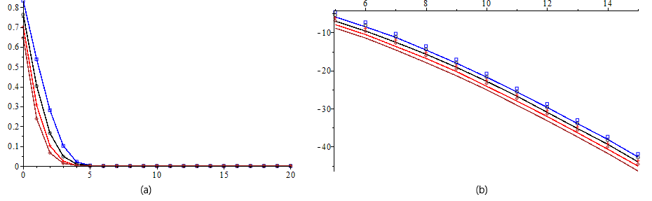
In this example we illustrate the decay rate of the eigenvalues (λnα​(c))(\lambda_{n}^{\alpha}(c)) given by theorem 3 for different values of α\alpha. In figure 1 (a), we have plotted the graph of (λnα​(c))(\lambda_{n}^{\alpha}(c)) and in figure 1 (b) we have plotted the graphs of l​o​g​(λnα​(c))log(\lambda_{n}^{\alpha}(c)) versus the graphs of −(2​n+1)​log⁡(4​n+4​α+2e​c)-(2n+1)\log\Big(\frac{4n+4\alpha+2}{ec}\Big)

Refer to caption
Figure 1: (a) Graph of λn(α)​(c)\lambda_{n}^{(\alpha)}(c)for α=1\alpha=1 (blue), α=1.5\alpha=1.5 (black), α=2\alpha=2 (red) and α=2.5\alpha=2.5 (brown) (b)Graph of log⁡(λn(α)​(c))\log(\lambda_{n}^{(\alpha)}(c))

Example 2: In this example, for a positive real number ss, we consider the Brownian motion function

Bs​(x)=∑k=1∞Xkks​cos⁡(k​π​x)x∈I=[−1,1]B_{s}(x)=\sum_{k=1}^{\infty}\frac{X_{k}}{k^{s}}\cos(k\pi x)\quad x\in I=[-1,1]

Here XkX_{k} is a sequence of independent standard Gaussian random variable. It is well known that Bs∈Hs′−1/2​(I),B_{s}\in H^{s^{\prime}-1/2}(I), for any s′<s−12.s^{\prime}<s-\frac{1}{2}. Here, Hs​(I)H^{s}(I) is the Sobolev space over I,I, with smoothness exponent s.s. For the special values of s=1.5s=1.5 and c=5​πc=5\pi, and the two values of N=46N=46 and N=90,N=90, we have computed SN​(Bs),S_{N}(B_{s}), the truncated series expansion to the order N,N, of BsB_{s} in the GPSWFs basis. We have found that

‖Bs−S46​(Bs)‖∞≈01​E−01,‖Bs−S90​(Bs)‖∞≈05​E−02.\|B_{s}-S_{46}(B_{s})\|_{\infty}\approx 01E-01,\qquad\|B_{s}-S_{90}(B_{s})\|_{\infty}\approx 05E-02.

Moreover, the graphs of BsB_{s} and of its approximation S90​BsS_{90}B_{s} are given by the figure 2.

Refer to caption
Figure 2: (a) Graph of Bs​(x)B_{s}(x) (b) graph of S90(α)​Bs​(x)S^{(\alpha)}_{90}B_{s}(x) (c) graph of the error EN=Bs​(x)−S90(α)​Bs,E_{N}=B_{s}(x)-S^{(\alpha)}_{90}B_{s}, with s=1.5s=1.5, N=90.N=90., c=5​πc=5\pi and α=1.5\alpha=1.5

Example 2:To illustrate approximation by GPSWFs we have considered the Weierstrass-Mondelbrot function given by :

Ms,λ​(x)=∑k=0∞sin⁡(λk​x)λk⁡(2−s)M_{s,\lambda}(x)=\sum_{k=0}^{\infty}\frac{\sin(\lambda^{k}x)}{\lambda^{k(2-s)}}

For λ>1\lambda>1 and s<1s<1, Ms,λ∈Hαs​(I)M_{s,\lambda}\in H^{s}_{\alpha}(I) In this example we have considered the values of α=0.5\alpha=0.5, c=5​πc=5\pi and N=95N=95 then we have computed the projection, over S​p​a​n​(ψ0,c(α),⋯,ψN,c(α))Span(\psi_{0,c}^{(\alpha)},\cdots,\psi_{N,c}^{(\alpha)}), SN​(Ms,λ​(x))S_{N}(M_{s,\lambda}(x)). For this purpose, we have computed the different expansion coefficients Cn​(Ms,λ​(x))=∫−11Ms,λ​(x)​ψn,c(α)​(y)​ωα​(y)​𝑑y\displaystyle{C_{n}(M_{s,\lambda}(x))=\int_{-1}^{1}M_{s,\lambda}(x)\psi_{n,c}^{(\alpha)}(y)\omega_{\alpha}(y)dy} which are exactly given thanks to (16). Since Ms,λM_{s,\lambda} is an odd function , C2​n​(Ms,λ)=C_{2n}(M_{s,\lambda})= . Moreover

C2​n+1​(Ms,λ)\displaystyle C_{2n+1}(M_{s,\lambda}) =\displaystyle= ∑ℓ=0∞β2​ℓ+12​m+1​∑k=0∞1λk⁡(2−s)​∫−11sin⁡(λk​x)​P^2​ℓ+1(α)​(x)​ωα​(x)​𝑑x\displaystyle\sum_{\ell=0}^{\infty}\beta_{2\ell+1}^{2m+1}\sum_{k=0}^{\infty}\frac{1}{\lambda^{k(2-s)}}\int_{-1}^{1}\sin(\lambda^{k}x)\hat{P}^{(\alpha)}_{2\ell+1}(x)\omega_{\alpha}(x)dx (61)
=\displaystyle= π​2α+12​∑ℓ=1∞(−1)ℓ​β2​ℓ+12​m+1​Γ⁡(2​ℓ+α+3)OPEN(​h2​ℓ+1)​Γ​(2​ℓ+1)​∑k=1∞λk⁡(s−α−5/2)​J2​ℓ+α+32​(λk)\displaystyle\sqrt{\pi}2^{\alpha+\frac{1}{2}}\sum_{\ell=1}^{\infty}(-1)^{\ell}\beta_{2\ell+1}^{2m+1}\frac{\Gamma(2\ell+\alpha+3)}{\sqrt{(}h_{2\ell+1})\Gamma(2\ell+1)}\sum_{k=1}^{\infty}\lambda^{k(s-\alpha-5/2)}J_{2\ell+\alpha+\frac{3}{2}}(\lambda^{k})

In figure 3 we have plotted the function M1,2M_{1,2} and the graph of the error M1,2−SN​(M1,2​(x))M_{1,2}-S_{N}(M_{1,2}(x))

Refer to caption
Figure 3: (a) Graph of M1,2M_{1,2} (b) graph of the error M1,2−SN​(M1.2)M_{1,2}-S_{N}(M_{1.2})

Moreover in table 1, we give the approximation error ‖Ms,2−SN(α)​(Ms,2)L2​(I,ωα)‖{\left\|{M_{s,2}-S_{N}^{(\alpha)}(M_{s,2})_{L^{2}(I,\omega_{\alpha})}}\right\|} of the Weierstrass-Mandelbrot function by GPSWFs for different values of s and α\alpha.

α\alpha s=0.25s=0.25 s=0.5s=0.5 s=0.75s=0.75 s=1s=1
0.10.1 1.69146​E−041.69146E-04 5.42800​E−045.42800E-04 1.74173​E−031.74173E-03 5.61554​E−0.35.61554E-0.3
0.50.5 1.90589​E−041.90589E-04 6.07253​E−046.07253E-04 1.93120​E−031.93120E-03 6.15556​E−0.36.15556E-0.3
11 2.12572​E−042.12572E-04 6.72661​E−046.72661E-04 2.12113​E−032.12113E-03 6.68912​E−0.36.68912E-0.3
1.51.5 2.30518​E−042.30518E-04 7.25472​E−047.25472E-04 2.27216​E−032.27216E-03 7.10411​E−037.10411E-03
2.02.0 2.45810​E−042.45810E-04 7.70063​E−047.70063E-04 2.39797​E−032.39797E-03 7.44278​E−037.44278E-03
Table 1: Values of the approximation of Weierstrass-Mandelbrot function ‖Ms,2−SN(α)​(Ms,2)L2​(I,ωα)‖{\left\|{M_{s,2}-S_{N}^{(\alpha)}(M_{s,2})_{L^{2}(I,\omega_{\alpha})}}\right\|} for different values of ss and α\alpha

References

  • [1] G. E. Andrews, R. Askey and R. Roy, Special Functions, Cambridge University Press , Cambridge, New York, 1999.
  • [2] J.Bergh,J.Lofstrom, Interpolation spaces.An introduction, Springer-Verlag , Cambridge, Berlin and New York, 1967.
  • [3] C.Bernardi, Y.Maday, Spectral methods, in P.G,J.L.Lions(Eds.),Handbook of Numerical Analysis ,Vol5, Techniques of Scientific computing, Elsevier, Amesterdam,1997,pp.209-486.
  • [4] A. Bonami and A. Karoui, Uniform bounds of prolate spheroidal wave functions and eigenvalues decay, C. R. Math. Acad. Sci. Paris. Ser. I, 352 (2014), 229–234.
  • [5] A. Bonami and A. Karoui, Uniform approximation and explicit estimates of the Prolate Spheroidal Wave Functions, Constr. Approx., 43 (2016), 15–45.
  • [6] A. Bonami and A. Karoui, Spectral decay of time and frequency limiting operator, Appl. Comput . Harmon. Anal., 42 (2017), 1–20.
  • [7] A. Bonami and A. Karoui, Approximation in Sobolev spaces by Prolate Spheroidal Wave Functions, Appl. Comput . Harmon. Anal 42, 361-377 (2017)
  • [8] A. Bonami, P.Jaming and A. Karoui, Non asymptotic behavior of the spectrum of the sinc kernel operator and related applications, available at arXiv:1804.01257, (2018).
  • [9] C.Canuto,A.Quarteroni, Approximation results for orthogonal polynomials in Sobolev spaaces,Math.Comp.38(1982)67-86.
  • [10] Q.Chen, D.Gottlieb,J.S Hesthaven, Spectral methods based on prolate spheroidal wave functions for hyperbolic PDEs, SIAM J Numer. Anal 43(5) (2005) 1912-1933
  • [11] Serge Nicaise, Jacobi Polynomials,weighted Sobolev spaces and approximation results of some singularities , Math.Nachr.213(2000),117-140
  • [12] B.Y.Guo, L.L.Wang, Jacobi approximations in non-uniformly Jacobi-weighted Sobolev spaces, J.Approx.Theory 128 (2004) 1-41
  • [13] A. Karoui and A. Souabni, Generalized Prolate Spheroidal Wave Functions: Spectral Analysis and Approximation of Almost Band-limited Functions, J. Four. Anal. Appl., 22 (2), (2016), 383–412.
  • [14] A. Karoui and A. Souabni Weighted Finite Fourier Transform Operator: Uniform Approximations of the Eigenfunctions, Eigenvalues Decay and Behaviour. J. Sci. Comp. 71 (2017), 547–570.
  • [15] H. J. Landau and H. O. Pollak, Prolate spheroidal wave functions, Fourier analysis and uncertainty-III. The dimension of space of essentially time-and band-limited signals, Bell System Tech. J. 41, (1962), 1295–1336.
  • [16] T. Moumni, On essentially time and Hankel band-limited function Integral transforms special functions, 23 (2), (2012), 83–95.
  • [17] Frank W. Olver, Daniel W. Lozier, Ronald F. Boisvert, and Charles W. Clark, NIST Handbook of Mathematical Functions, Cambridge University Press, New York, NY, USA, 1st edition, 2010.
  • [18] D. Slepian and H. O. Pollak, Prolate spheroidal wave functions, Fourier analysis and uncertainty I, Bell System Tech. J. 40 (1961), 43–64.
  • [19] D. Slepian, Prolate spheroidal wave functions, Fourier analysis and uncertainty–IV: Extensions to many dimensions; generalized prolate spheroidal functions, Bell System Tech. J. 43 (1964), 3009–3057.
  • [20] G. Szegö, Orthogonal polynomials, Fourth edition, American Mathematical Society, Colloquium Publications, Vol. XXIII. American Mathematical Society, Providence, R.I., 1975.
  • [21] L. L. Wang and J. Zhang, A new generalization of the PSWFs with applications to spectral approximations on quasi-uniform grids, Appl. Comput. Harmon. Anal. 29, (2010), 303–329.
  • [22] Batir, N. Inequalities for the gamma function. Arch. Math. 91, 554–563 (2008).