The topological susceptibility of two-dimensional gauge theories
Abstract
In this paper we study the topological susceptibility of two-dimensional gauge theories. We provide explicit expressions for the partition function and the topological susceptibility at finite lattice spacing and finite volume. We then examine the particularly simple case of the abelian theory, the continuum limit, the infinite volume limit, and we finally discuss the large limit of our results.
I Introduction
The study of -dependence of QCD by means of lattice simulations has been the subject of several recent studies, mainly triggered by the possible implications for axion physics Berkowitz:2015aua; Kitano:2015fla; Borsanyi:2015cka; Trunin:2015yda; Bonati:2015vqz; Petreczky:2016vrs; Frison:2016vuc; Borsanyi:2016ksw; Burger:2018fvb. It is however well known that Monte Carlo algorithms typically used in numerical simulations suffer from a severe critical slowing down as the continuum limit is approached, with autocorrelation times of topological observables that grow about exponentially in the inverse of the lattice spacing Alles:1996vn; DelDebbio:2002xa; DelDebbio:2004xh; Schaefer:2010hu. This led to the development of new algorithms, specifically devised to improve the sampling of topologically nontrivial configuration Vicari:1992jy; Luscher:2011kk; Mages:2015scv; Laio:2015era; Bietenholz:2015rsa; Frison:2016vuc; Borsanyi:2016ksw; Hasenbusch:2017unr; Bonati:2017woi; Bonati:2017nhe; Bonati:2018blm; Bonanno:2018xtd.
From a general point of view, it is very useful to have the possibility of performing quantitative checks of the Monte Carlo results against exact ones. This is obviously not possible in the general case, however simplified (toy) models sometimes exist that are analytically soluble but still complicated enough to be used as nontrivial test beds. In statistical physics the two-dimensional Ising model is probably the most popular choice FerrenbergLandauWong, while in field theory two-dimensional lattice gauge theories are the natural playground for tests of numerical simulations: on one side they are computationally much cheaper than their four dimensional counterparts, on the other side it is possible to determine many exact results that may constitute precise benchmarks for numerical results and extrapolations.
The present paper is devoted to the extension of known analytic results concerning two-dimensional lattice gauge theories in the absence of a term to the case when such a term is present, and more specifically to the evaluation of the topological susceptibility, for finite volumes and for generic values of the coupling . Finite volume results at fixed coupling may be especially useful because they allow direct comparison with simulations without the need of extrapolating to infinite volume and to the continuum limit.
The paper is organized as follows: Section II is devoted to a summary of known results, with special emphasis on finite lattices with spherical and toroidal geometries. In Section III we fix our notation trying to make correspondence with previous literature as far as possible, and we give our definitions for the density of topological charge and for the topological susceptibility in gauge theories, exploiting the existence of the subgroup. We present our general formulas for the partition function in the presence of a term and for the topological susceptibility, for generic values of , and , and for any genus of the lattice manifold, showing explicitly that the periodicity of the partition function for shifts of the parameter is preserved. In Section IV we focus on the case where many closed-form expressions can be explicitly found for generic values of and can be compared with partial results already available in the literature. Strong evidence of precocious scaling by using a renormalized coupling is also exhibited. In Section V we analyze the (finite volume) continuum limit of the model in the presence of a term. In Section VI the infinite volume limit of the topological susceptibility is discussed in detail. Section VII is devoted to the study of the large limit in the infinite and finite volume cases (with further evidence of precocious scaling) and to numerical checks of our large results.
II A summary of known results
The finite volume lattice version of gauge theories most widely studied in the literature is defined by the following partition function Bars:1979xb:
| (1) | |||
| (2) |
where unitary matrices are attached to the links of the lattice and are the ordered products of the link matrices along any lattice plaquette. is the lattice ’t Hooft coupling, whose relationship with the standard (dimensionful) coupling11 1 In the following we will denote by also the genus of the manifold on which the theory is defined; the meaning of should however be clear from the context. is , where is the lattice spacing and the volume is given by . The sum in Eq. (2) runs over all plaquettes, while the integration involves all link variables and is performed by using the Haar measure for the group. Due to its crucial role we recall that, when the integrand involves only functions of the eigenvalues of the integration variable, the Haar measure reduces to (see e.g. Drouffe:1983fv)
| (3) |
where
| (4) |
The peculiarity of two dimensional models consists in the possibility of performing a change of integration variables (exploiting the invariance of the Haar measure) in such a way that most nontrivial integrations involve directly the plaquette matrices. That this is a feasible strategy can be understood, for a two dimensional compact orientable manifold without boundary, by using the Euler characteristic , where is the number of sites (vertices) of the lattice and is the genus of the lattice manifold. The maximal number of links that can be gauged away (maximal tree) is simply and therefore the number of nontrivial integration variables is .
Two cases particularly useful for applications are the manifolds with the topology of the sphere () and the manifolds with the topology of the torus (). For the case we have , implying that one of the plaquette variables may be expressed as a function (actually the product) of all other matrices; in this case one can easily prove the equivalence of these models to the chiral chains of length (see also later in this section), in order to use the results available for these systems Brower:1980rp; Brower:1980vm. For (the manifolds typically adopted in simulations) we get and the independent variables may be chosen to be plaquettes and two other degrees of freedom (“torons”). Integration over the torons may be explicitly carried out Kiskis:2014lwa, and the result leads again to the possibility of expressing the last plaquette as the product of all other variables. This procedure can be generalized without difficulties also to the case of generic topology.
Without belaboring the details we only quote the final result, due to Rusakov Rusakov:1990rs (see also Kiskis:2014lwa for the case of the torus): the partition function corresponding to a compact orientable lattice manifold of genus without boundary is:
| (5) |
where , the sum runs over all representations of , is the dimension of the representation and Drouffe:1983fv
| (6) |
with the character of . If the manifold is nonorientable the partition function is always equal to 1, if fixed boundaries are present the result depends on the holonomies associated to the boundaries Rusakov:1990rs. When the boundary holonomies are fixed to be trivial, one obtains again Eq. (5) and this is a possible way of proving the equivalence of the spherical topology with chiral chains. We explicitly note that, when writing expressions like Eq. (5), we must keep in mind that the number of links belonging to each plaquette is not a priori fixed, and for small values of it must be large enough to ensure the possibility of imposing boundary conditions compatible with the genus of the lattice manifold. In particular for the plaquettes must be polygons with at least sides.
It is worth noticing that, due to the invariance properties of the measure, a simple result may be obtained in the case , :
| (7) |
We also recall that the continuum partition function in the case of a finite (dimensionless) area can be obtained starting from the heat kernel action, corresponding to the replacement22 2 There is sometimes confusion in the literature on the numerical factor appearing in the exponent, which depends on the conventions adopted in the action. We checked that Eq. (8) is the correct large limit of Eq. (13). Drouffe:1983fv
| (8) |
where is the quadratic Casimir in the representation and the result is
| (9) |
The infinite volume limit of Eq. (5) can be easily recovered in different ways. For instance one may observe that when it is consistent to choose an axial gauge condition, amounting to setting for all the links in the “time” direction of the lattice. Factorization of the integrals in Eq. (2) follows trivially, implying a direct relationship with the single plaquette model:
| (10) |
where
| (11) |
and the properties of the trivial representation ( and ) have been exploited. It is important to stress that the same result might have been obtained by observing that the quantities can be explicitly computed for all values of . Indeed by recalling the definition of the modified Bessel functions of integer order
| (12) |
it is possible to obtain the result Drouffe:1983fv
| (13) |
where the indices () parametrize the representation; in particular Bars:1979xb
| (14) |
Noticing that for all and for all finite real values of , it is easy to get convinced that
| (15) |
for all and for all finite values of . This observation implies Eq. (10) and also that the convergence to the infinite volume limit is exponentially fast for large values of .
As we mentioned in the introduction, many exact results have been obtained in the past with regard to the large limit of many matrix models. For a general review we refer to Rossi:1996hs, quoting here only the existence of a third order phase transition at , first identified by Gross and Witten Gross:1980he and Wadia Wadia:1980cp, the computation of the first few corrections of the free energy Goldschmidt:1979hq, the exact expression for the large eigenvalue distribution of the plaquette variable for the single plaquette Gross:1980he and for the chiral chains with and Brower:1980rp; Brower:1980vm; Friedan:1980tu, the solution of the external field problem for all Brower:1980tb; Brower:1980rp; Brower:1980vm; Brezin:1980rk and the expectation value of for the single plaquette model Rossi:1982vw.
III Topological charge and susceptibility
The existence of a topological charge in two dimensional gauge theories is related to the existence of a Abelian subgroup, that can be parametrized by a phase , related to the determinant of the matrix by the relationship
| (16) |
It is easy to get convinced that on a compact orientable lattice manifold without boundaries the following property holds
| (17) |
where is the phase associated with the determinant of each plaquette variable. Hence a simple definition for the topological charge density associated with each plaquette is
| (18) |
the total topological charge is and, because of the above property of , can only take integer values. Note that the second equality in Eq. (18) holds only for an appropriate and -dependent choice of the branch cuts. If however the standard branch is used (as will always be done in the following), the two expressions for the topological charge are generically different, but nevertheless the corresponding -dependent partition functions are the same.
By definition the (dimensionless) topological susceptibility is
| (19) |
where the expectation values are to be computed at . The lattice representation of follows trivially from the above results, recalling that , and simple parity arguments imply that , therefore in practice we just have to compute .
The -dependent partition function can be defined as
| (20) |
and in order to compute we can repeat and adapt Rusakov’s procedure. Let us define the quantities
| (21) |
with the property that
| (22) |
By choosing an appropriate gauge condition and performing the residual nontrivial integrations we then obtain our general result for the -dependent partition function:
| (23) |
Noticing that , where are the eigenvalues of , and defining the functions
| (24) |
which for integer indices reduces to modified Bessel functions (see Eq. (12)), we obtain the closed form expression
| (25) |
using arguments identical to those needed to prove Eqs. (13) and (14) Bars:1979xb; Gross:1980he; Drouffe:1983fv.
From this expression it follows that is equivalent to where ; as a consequence, when performing the summation over all representations, each contribution appearing in has an identical counterpart in the expression of , implying exact periodicity in for all values of and . We consider this to be a quite nontrivial evidence for the correct normalization of the topological charge in the two dimensional gauge theories.
In order to simplify the notation it is convenient to introduce the weights
| (26) |
with the property that . Starting from the formal expression for the topological susceptibility:
| (27) |
it is then possible to represent in the form
| (28) | ||||
where we have defined
| (29) | ||||
and
| (30) | ||||
which can be rewritten as sums of determinants involving modified Bessel functions and related functions (see Sec. VI for more details on the simplest case). In the derivation of Eq. (28) we have also exploited the fact that vanishes at , which is equivalent to
| (31) |
The proof of this identity rests on the cancellation of the contributions coming from each representation (associated to ) and its conjugate representation (associated to ), indeed
| (32) |
from which it follows .
By the same arguments applied in the previous Section, and observing that for obvious symmetry reasons, we may conclude that also the convergence of the topological susceptibility to its infinite volume limit is exponentially fast. An example of the finite volume behaviour of the topological susceptibility is shown in Fig. 1 for the case.

A peculiar property of the case , (the two-link chiral chain) is
| (33) |
implied by the trivial relationship .
It is also quite interesting to study the limit of the theory. Since appears in the exponent of in the weights Eq. (26), all representations with disappear as and only the representations labelled by give a finite contribution in this limit. The relevant representations are therefore identified by a single index , running from to , and the partition function is simply
| (34) |
where the explicit form of the characters has been used (see Drouffe:1983fv) and
| (35) |
where the average stands for the average in the single plaquette model at . The topological susceptibility of the theory is shown in Fig. 1 for the case. Further aspects of the large behaviour will be discussed in Sec. V and Sec. VII.
To better understand the form of Eq. (28) it is convenient to further generalize the problem, by introducing plaquette dependent lattice coupling and angle. It is immediate to verify that the Rusakov result can be generalized to this case and the partition function becomes
| (36) |
We can now write a formal expression for the two-point correlation function of the topological charge by using
| (37) |
and it is simple to verify that has the form
| (38) | ||||
which expresses the fact that in two dimensions the correlator takes just two values. These values are obviously related to the expressions appearing in Eq. (28), that can indeed be rewritten in the form
| (39) |
This is nothing but the general relation between the susceptibility and the two point function, written in the case in which assumes only two values. Since , it is simple to show that goes to zero exponentially in (the dimensionless volume) as the thermodynamic limit is approached; in this limit the two point function of the topological charge reduces to a function.
IV The case
In the purely Abelian case many simplifications occur, due to the commutativity of the matrices. In particular there is no dependence on the genus of the manifold, as one can easily see by noticing that all the representations have dimension 1.
The topological charge density is simply (where is the Abelian phase of the plaquette) and the character of the -th representation of is just . As a consequence one may compute directly the dependent partition function on a finite lattice obtaining
| (40) |
The weights are simply
| (41) |
The resulting expression for the finite volume topological susceptibility is then
| (42) | ||||
where we introduced the auxiliary functions
| (43) | ||||
| (44) | ||||
The typical behaviour of as a function of and is shown in Fig. 2(a). In Fig. 2(b) one may observe the precocious scaling exhibited by the ratio , when we parametrize the dependence on the coupling by means of the combination , corresponding to a physical dimensionless quantity in the continuum limit (where it takes the asymptotic value ). Precocious scaling by use of renormalized couplings was observed in a different context in references tadpole; Lepage:1992xa.


The finite volume continuum limit of the dependent partition function in the case is
| (45) |
where we dropped the independent multiplicative factor . A corresponding expression for the topological susceptibility can easily be obtained, which can be written in the form
| (46) |
where . In order to compare with continuum results (see e.g. Cao:2013na), it must be kept in mind that in the case to preserve the canonical normalization of the fields (see also the note at the end of Section II).
In the infinite volume limit the dominant term of the sum in Eq. (40) is the one corresponding to the minimum value of , and we thus see the emergence of a multi-branched structure
| (47) |
with the partition function being non-analytic at the odd multiples of . This phenomenon persists also when considering the infinite volume limit of the continuum version of the model discussed above. The presence of these first order transition points prevents a simple factorization of the form Eq. (10) from being applicable for generic values, indeed a naive application of factorization would give
| (48) |
which is non periodic in . It is however important to stress that, as far as we consider , all the expressions obtained by using the single plaquette model correctly describe the limit of the -plaquette model. In particular the infinite volume topological susceptibility is given by
| (49) |
V The continuum limit
The continuum limit of two dimensional gauge theories is simply the limit because the coupling is dimensionful and therefore the above limit is the same as the limit . By generalizing the arguments that lead to Eq. (13) we may obtain the following representation for the functions appearing in :
| (50) | ||||
In the limit one may replace with and perform the resulting gaussian integration, thus obtaining
| (51) |
where the common factor does not depend on .
A few straightforward manipulations allow to represent the above result in the form
| (52) | ||||
The determinant can be computed in the limit , obtaining the result
| (53) |
where is another common factor independent of , and it is possible to verify that the product is nothing but the asymptotic form of in the large limit, hence it is a lattice artifact that can be ignored when analyzing the continuum properties of the model.
We recall that is the quadratic Casimir of the representation, as expected from the result Eq. (8). We report here, for the convenience of the reader, the known explicit form of and :
| (54) | ||||
The continuum limit of the partition function on a manifold with (dimensionless) area is therefore
| (55) |
and the continuum limit of the weights defined in Eq. (26) is
| (56) |
An immediate consequence of the above results is the possibility of evaluating the finite volume continuum limit of the topological susceptibility:
| (57) |
which in the infinite volume limit does not depend on the genus and becomes simply
| (58) |
for all , because when .
It is important to note that the continuum expression for the partition function is consistent with the previously proven periodicity in with period of the partition function. Let’s focus on the exponents appearing in Eq. (55) and notice that they can be rewritten in the form
| (59) | ||||
also in the continuum is thus equivalent to where . Since the periodicity of the continuum partition function Eq. (55) follows as in Sec. III.
The continuum version of the limit is simply
| (60) |
and one may appreciate that it turns out to be independent of and therefore coincident with the continuum version of the model. However we notice that, contrary to naive expectations, the finite volume continuum limit will not in general coincide with its value, and will depend on and , with the notable exception of the large limit, to be discussed in Sec. VII.
The properties of the finite volume continuum limit will be discussed in detail in a forthcoming publication.
VI The infinite volume limit
We assume in this section (see the discussion in Sec. IV), in order to exploit the large volume factorization also at , obtaining for all genuses
| (61) |
where
| (62) | ||||
Computing the infinite volume topological susceptibility thus amounts to evaluating the quantity
| (63) |
where we exploited the fact that and the property
| (64) |
in the limit . may be evaluated starting from
| (65) |
and it can be seen (using again arguments analogous to those of Bars:1979xb; Gross:1980he; Drouffe:1983fv) that may be expressed as the sum of the determinants obtained from by replacing one of the lines with and two different lines with . Using these expressions it is straightforward to numerically compute and in Fig. 3 we show the results obtained for and ; two different regimes are clearly visible in this figure, which will be discussed in depth in Sec. VII.

VII The large limit
In the large limit analytic calculations are made possible by the fact that the functional integral is dominated by the saddle point configuration of the fields, which in turn can be found by solving the appropriate (saddle point) equations for the eigenvalues of a matrix variable. In practice one must replace the summations over the index “” with an integration in the variable , weighted by an eigenvalue density , normalized to .
Explicit eigenvalue densities have been found for the infinite volume case (equivalent to the single plaquette) Gross:1980he, and for the chiral chains with Brower:1980rp; Brower:1980vm, and the corresponding free energies have been computed. In all cases a third order phase transition is present, and therefore one needs to know the separate expressions for the strong and weak coupling eigenvalue distributions. As we saw in the previous sections, as far as we are interested in the topological susceptibility (or in other properties related to the behaviour of the free energy close to ) we can use the single plaquette model to compute values in the thermodynamic limit.
In the single plaquette model the transition occurs at and the eigenvalue density is Gross:1980he
| (66) |
where and
| (67) | ||||
| (68) |
In order to extend these results to the evaluation of the large limit of the topological susceptibility at infinite volume we must replace the saddle point equation introduced in Gross:1980he with
| (69) |
where we introduced the scaling variable in order to obtain a consistent large limit, in analogy with the procedure adopted in Bonati:2016tvi; Rossi:2016uce following the original proposal by Witten Witten:1980sp. We may introduce in the saddle point equation the Ansatz
| (70) |
where is the eigenvalue density Eq. (66) found in Gross:1980he, while must be an odd function of satisfying the equation
| (71) |
If we denote by the free energy of the system, its -dependent part is therefore33 3 This expression is clearly non -periodic in , as a consequence of the use of the single plaquette model.
| (72) |
with the factor coming from the partial cancellation of the two terms in the free energy that are quadratic in , i.e. the -term and the term coming from the Haar measure. In the large limit the above expression is finite while all contributions of higher order in are depressed by powers of . Hence we immediately obtain the large relationship
| (73) |

Notice that the equation defining may depend on only through the limits of the integration domain, which in turn should not change with respect to the domain of , because all change in would be depressed by a power of . This observation implies that special care will be needed in the strong coupling region, because with no apparent dependence on , but the formal solution for is
| (74) |
implying a nonintegrable singularity around . It is easy to get convinced that the resulting singular behavior may be parametrized by
| (75) |
where
| (76) | ||||
and is a regular function connected to the dependent cutoff scale, which is in turn related to the behavior of the density in the proximity of . On these grounds, since when , we find
| (77) |
which shows the correct limit and exhibits a divergence in the limit , as required in order to match the weak coupling behavior.
In the weak coupling regime the solution of Eq. (71) is
| (78) |
the integral in Eq. (73) is convergent and we get (using Eq. 3.842.2 of GradshteynRyzhik)
| (79) |
This result can be easily obtained also without explicitly solving the saddle point equation, because from the definition of the topological charge we have
| (80) |
and in Rossi:1982vw it has been proven that, at in the weak coupling phase of the single plaquette model, we have
| (81) |
this was further strengthened in Aneva:1983za by showing that
| (82) |
Hence we may establish the relationship, holding for all and
| (83) |
implying immediately
| (84) |
This result reproduces the correct large behavior of the susceptibility and shows a divergence for , needed in order to match the strong coupling behavior. Notice that, due to the singularity in , this argument could not be applied to the strong coupling phase, where it is known that is proportional to and behaves like when Green:1980bs; Green:1981mx; Rossi:1982vw.
The numerical evaluation of , even for quite small values of , shows surprisingly good agreement with the above predictions, as shown in Fig. (4).

The above results are restricted to the infinite volume version of the models, but they may be employed in the limit in order to obtain for this case expressions holding also in the finite volume large limit, at least in the weak coupling regime. Indeed by trivially extending Eq. (82) to include the dependence on and substituting the results in Eqs. (34)-(35) one easily obtains for large :
| (85) |
This expression can be rewritten in the form
| (86) |
where is the partition function of the single plaquette model (see Sec. IV) and therefore
| (87) |
where now
| (88) |
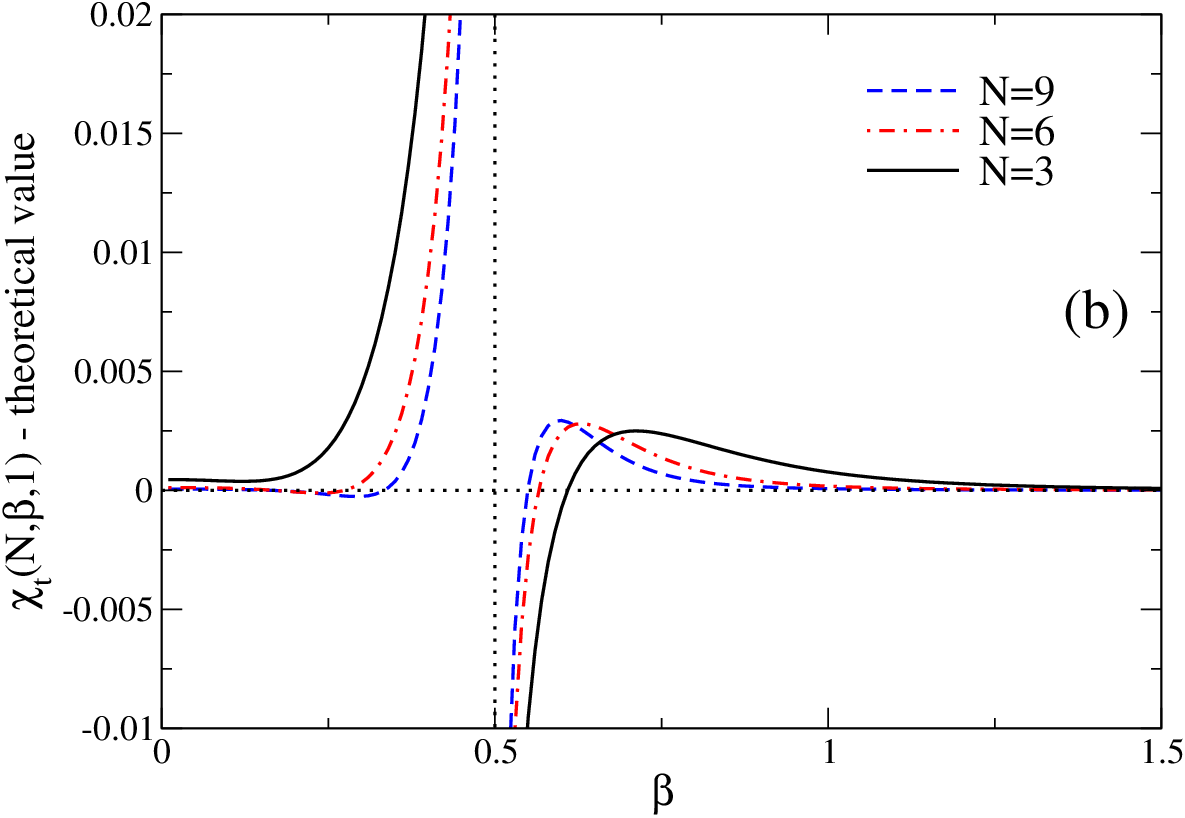
Here is the value Eq. (79) of the large limit of the topological susceptibility in the weak coupling regime, from which we may appreciate that in the continuum limit . It is worth noticing that very precocious large scaling is obtained when studying as a function of the dimensionless variable , which is the finite- analogous of , see Fig. 5. This is analogous to what was previously observed in the case of , shown in Fig. 2.
Another important comment concerns the dependence of the large finite volume susceptibility on . It is possible to show that the same results holds true not only for , but also for all values, because representations with get suppressed as (see Eq. (26)). On the other hand it can not hold in the case , since we know that for all and, as a consequence, it vanishes also in the limit.
By generalizing to general the arguments put forward by Douglas and Kazakov Douglas:1993iia one may argue that the finite area transition they found is present only in the case, and it would be interesting to investigate whether this transition may affect the topological susceptibility.
VIII Conclusions
In this paper we studied the dependence of two dimensional gauge theories, providing explicit expressions for the topological susceptibility in the most general setting, i.e. at finite volume, finite lattice spacing and for a generic topology of the space-time manifold.
These expressions can be simplified in several different ways by restricting to more specific cases. In particular we analyzed the thermodynamic limit at fixed (’t Hooft) coupling and the continuum limit at fixed dimensionless volume, the case of the abelian theory being particularly simple. We finally addressed the large limit of the results obtained at infinite volume, showing that the large behaviour of the topological susceptibility is completely different for and for . These two regions correspond to the strong and weak coupling phases of the theory, separated by the Gross-Witten-Wadia transition.
From the practical point of view our results can be useful to benchmark, in two dimensional gauge theories, new Monte-Carlo algorithms specifically targeted at improving the decorrelation of topological modes in lattice gauge theories. From the theoretical side the most significant results obtained are probably the determination of the continuum dependent partition function on a manifold of arbitrary genus and the large limit (at infinite volume) of the topological susceptibility for arbitrary coupling.
A remarkable aspect of our large computation is the fact that the term is sub-leading in the action, but nevertheless we have been able to compute the topological susceptibility at large using the saddle-point approximation method, whose range of applicability is typically restricted to leading order computations. This is analogous to what has been done in Rossi:2016uce for two dimensional models, but the present case is probably more surprising since the topological susceptibility does not vanish in the large limit.
Putting together the two arguments presented in Sec. VII to justify Eq. (79) we obtain a new and completely independent proof of Eq. (81), suggested in Green:1980bs; Green:1981mx and proven in Rossi:1982vw, and of Eq. (82), proven in Aneva:1983za. A natural question is whether the new proof can be extended to other cases that were not tractable with the previously known methods.
Acknowledgement It is a pleasure to thank M. D’Elia for useful discussions.
References
- (1) E. Berkowitz, M. I. Buchoff and E. Rinaldi, Phys. Rev. D 92, 034507 (2015) [arXiv:1505.07455 [hep-ph]].
- (2) R. Kitano and N. Yamada, JHEP 1510, 136 (2015) [arXiv:1506.00370 [hep-ph]].
- (3) S. Borsanyi et al., Phys. Lett. B 752, 175 (2016) [arXiv:1508.06917 [hep-lat]].
- (4) A. Trunin, F. Burger, E.-M. Ilgenfritz, M. P. Lombardo and M. Müller-Preussker, arXiv:1510.02265 [hep-lat].
- (5) C. Bonati, M. D’Elia, M. Mariti, G. Martinelli, M. Mesiti, F. Negro, F. Sanfilippo and G. Villadoro, JHEP 1603, 155 (2016) [arXiv:1512.06746 [hep-lat]].
- (6) P. Petreczky, H. P. Schadler and S. Sharma, Phys. Lett. B 762, 498 (2016) [arXiv:1606.03145 [hep-lat]].
- (7) J. Frison, R. Kitano, H. Matsufuru, S. Mori and N. Yamada, JHEP 1609, 021 (2016) [arXiv:1606.07175 [hep-lat]].
- (8) S. Borsanyi et al., Nature 539, 7627, 69 (2016) [arXiv:1606.07494 [hep-lat]].
- (9) F. Burger, E. M. Ilgenfritz, M. P. Lombardo and A. Trunin, Phys. Rev. D 98, 094501 (2018) [arXiv:1805.06001 [hep-lat]].
- (10) B. Alles, G. Boyd, M. D’Elia, A. Di Giacomo and E. Vicari, Phys. Lett. B 389, 107 (1996) [hep-lat/9607049].
- (11) L. Del Debbio, H. Panagopoulos and E. Vicari, JHEP 0208, 044 (2002) [hep-th/0204125].
- (12) L. Del Debbio, G. M. Manca and E. Vicari, Phys. Lett. B 594, 315 (2004) [hep-lat/0403001].
- (13) S. Schaefer et al. [ALPHA Collaboration], Nucl. Phys. B 845, 93 (2011) [arXiv:1009.5228 [hep-lat]].
- (14) E. Vicari, Phys. Lett. B 309, 139 (1993) [hep-lat/9209025].
- (15) M. Luscher and S. Schaefer, JHEP 1107, 036 (2011) [arXiv:1105.4749 [hep-lat]].
- (16) S. Mages, B. C. Toth, S. Borsanyi, Z. Fodor, S. D. Katz and K. K. Szabo, Phys. Rev. D 95, 094512 (2017) [arXiv:1512.06804 [hep-lat]].
- (17) A. Laio, G. Martinelli and F. Sanfilippo, JHEP 1607, 089 (2016) [arXiv:1508.07270 [hep-lat]].
- (18) W. Bietenholz, P. de Forcrand and U. Gerber, JHEP 1512, 070 (2015) [arXiv:1509.06433 [hep-lat]].
- (19) M. Hasenbusch, Phys. Rev. D 96, 054504 (2017) [arXiv:1706.04443 [hep-lat]].
- (20) C. Bonati and M. D’Elia, Phys. Rev. E 98, 013308 (2018) [arXiv:1709.10034 [hep-lat]].
- (21) C. Bonati, EPJ Web Conf. 175, 01011 (2018) [arXiv:1710.06410 [hep-lat]].
- (22) C. Bonati, M. D’Elia, G. Martinelli, F. Negro, F. Sanfilippo and A. Todaro, JHEP 1811, 170 (2018) [arXiv:1807.07954 [hep-lat]].
- (23) C. Bonanno, C. Bonati and M. D’Elia, JHEP 1901, 003 (2019) [arXiv:1807.11357 [hep-lat]].
- (24) A. M. Ferrenberg, D. P. Landau and Y. Joanna Wong Phys. Rev. Lett. 69, 3382 (1992)
- (25) I. Bars and F. Green, Phys. Rev. D 20, 3311 (1979).
- (26) J. M. Drouffe and J. B. Zuber, Phys. Rept. 102, 1 (1983).
- (27) R. C. Brower, P. Rossi and C. I. Tan, Phys. Rev. D 23, 942 (1981).
- (28) R. Brower, P. Rossi and C. I. Tan, Phys. Rev. D 23, 953 (1981).
- (29) J. Kiskis, R. Narayanan and D. Sigdel, Phys. Rev. D 89, 085031 (2014) [arXiv:1403.1770 [hep-th]].
- (30) B. E. Rusakov, Mod. Phys. Lett. A 5, 693 (1990).
- (31) P. Rossi, M. Campostrini and E. Vicari, Phys. Rept. 302, 143 (1998) [hep-lat/9609003].
- (32) D. J. Gross and E. Witten, Phys. Rev. D 21, 446 (1980).
- (33) S. R. Wadia, Phys. Lett. 93B, 403 (1980).
- (34) Y. Y. Goldschmidt, J. Math. Phys. 21, 1842 (1980).
- (35) D. Friedan, Commun. Math. Phys. 78, 353 (1981).
- (36) R. C. Brower and M. Nauenberg, Nucl. Phys. B 180, 221 (1981).
- (37) E. Brezin and D. J. Gross, Phys. Lett. 97B, 120 (1980).
- (38) P. Rossi, Phys. Lett. 117B, 72 (1982).
- (39) G. Parisi in Proceedings of the XXth International Conference on High Energy Physics, Madison (1980), L. Durand and L. G. Pondrom (eds.) American Institute of Physics, New York (1981).
- (40) G. P. Lepage and P. B. Mackenzie, Phys. Rev. D 48, 2250 (1993) [hep-lat/9209022].
- (41) C. Cao, M. van Caspel and A. R. Zhitnitsky, Phys. Rev. D 87, 105012 (2013) [arXiv:1301.1706 [hep-th]].
- (42) P. Rossi, Phys. Rev. D 94, 4, 045013 (2016) [arXiv:1606.07252 [hep-th]].
- (43) C. Bonati, M. D’Elia, P. Rossi and E. Vicari, Phys. Rev. D 94, 085017 (2016) [arXiv:1607.06360 [hep-lat]].
- (44) E. Witten, Annals Phys. 128, 363 (1980).
- (45) I. S. Gradshteyn and I. M. Ryzhik “Table of integrals, series and products” Academic Press (2007).
- (46) B. Aneva, Y. Brihaye and P. Rossi, Phys. Lett. 133B, 215 (1983).
- (47) F. Green and S. Samuel, Phys. Lett. B 103, 48 (1981).
- (48) F. Green and S. Samuel, Nucl. Phys. B 194, 107 (1982).
- (49) M. R. Douglas and V. A. Kazakov, Phys. Lett. B 319, 219 (1993) [hep-th/9305047].