Interplay between magnetic and superconducting fluctuations in the doped 2D Hubbard model: a parquet equations study
Abstract
We study the Hubbard model on a square lattice, using the parquet dynamical vertex approximation and the parquet approximation. These methods allow us to describe the mutual interference of spin-fluctuations in the particle-hole channel and superconducting fluctuations in the cooperon channel in an unbiased way. For small dopings we find predominant commensurable antiferromagnetic spin- and -wave superconducting fluctuations; for larger doping incommensurate antiferromagnetic spin fluctuations are concomitant to spin-triplet odd-frequency -wave superconducting fluctuations which are also supported by the dynamical structure of the pairing vertex.
pacs
71.10.Fd, 74.20.-z, 74.25.DwI Introduction
Unconventional superconductivity is not conventional in many respects. First of all, the critical temperatures are often high, which means several ten up to one hundred Kelvin. Second, the materials such as cuprates, Bednorz and Müller 1986; Dagotto 1994 ruthenates,Maeno et al. 1994; Mackenzie and Maeno 2003 and iron pnictides Kamihara et al. 2006; Wang et al. 2008 are special: they belong to the class of strongly correlated electron systems where a strong Coulomb interaction prevents a simple one-particle description. Correlations between the electrons need to be considered. Third, the symmetry of the order parameter is rather unusual. Instead of a simple -wave symmetry as in conventional, phonon-based superconductors, -Wollman et al. 1993; Shen et al. 1993; Tsuei et al. 1994; Maki 1998, -Maeno et al. 1994; Sigrist et al. 1999; Mackenzie and Maeno 2003 or -wave symmetriesMazin et al. 2008; Kuroki et al. 2008; Ikeda et al. 2010; Hanaguri et al. 2010; Hirschfeld et al. 2011; Kalenyuk et al. 2018 have been suggested and observed.
The latter two facts are strongly related to each other. In contrast to the phonon-mediated conventional superconductivity, unconventional superconductors are considered to occur due to the repulsive Coulomb interaction. Therefore even if spin fluctuations Scalapino 2012 or other microscopic mechanisms generate some attraction between the electrons, it cannot be local and instantaneous. The consequence is unconventional symmetry of the order parameter instead of a plain vanilla (even-frequency) -wave.
The theoretical description of high-temperature superconductivity has been—and still is—a challenge. It is pretty much established by now that one of the fundamental models for high-temperature superconductivity, the Hubbard model, indeed shows antiferromagnetism, pseudogaps, and -wave superconductivity. This has been demonstrated by a number of complementary methods such as quantum Monte-Carlo simulations,White et al. 1989a; White et al. 1989b; Bulut et al. 1993; Scalapino 1999; Bulut 2002 the functional-renormalization group (fRG), Zanchi and Schulz 1998; Halboth and Metzner 2000a; Halboth and Metzner 2000b; Honerkamp 2001; Honerkamp et al. 2001; Metzner et al. 2012, the fluctuation-exchange approximation (FLEX), Bickers et al. 1989; Moriya et al. 1990; Manske 2004, the variational cluster approximation Hanke et al. 2006 the two-particle self-consistent theory, Kyung et al. 2003 cluster Lichtenstein and Katsnelson 2000; Maier et al. 2005a; Maier et al. 2005b; Capone and Kotliar 2006; Haule and Kotliar 2007; Sordi et al. 2012; Gull et al. 2013 and diagrammatic extensions Toschi et al. 2007; Rubtsov et al. 2009; Katanin et al. 2009; Hafermann et al. 2009; Otsuki et al. 2014; Taranto et al. 2014; Kitatani et al. 2015; Kitatani et al. 2017; Ayral and Parcollet 2015; Gukelberger et al. 2017; Vučičević et al. 2017; Kitatani et al. 2019; Rohringer et al. 2018 of dynamical mean field theory (DMFT). In the far overdoped region, -wave superconductivity is not stable any longer. Since an interacting fermion system is however prone to all kinds of instabilities at low temperatures, one expects another kind of magnetic or superconducting instability at larger doping. One out of several possible candidates is -wave superconductivity, which has been studied to a limited extent in Refs. White et al. 1989b; Aligia et al. 1998; Rømer et al. 2015; Kitatani et al. 2017.
In the present paper, we study the two-dimensional Hubbard model on a square lattice, employing the parquet approximation (PA) Diatlov et al. 1957; De Dominicis 1962; De Dominicis and Martin 1964 and the dynamical vertex approximation (DA)Toschi et al. 2007; Rohringer et al. 2018 in its parquet variant.Valli et al. 2015; Li et al. 2016; Pudleiner et al. 2019a; Pudleiner et al. 2019b; Kauch et al. 2020 This is the first study of a lattice model out of half filling with the parquet variant of DA. In contrast to previous diagrammatic extensions of DMFT, Rubtsov et al. 2009; Katanin et al. 2009; Hafermann et al. 2009; Otsuki et al. 2014; Taranto et al. 2014; Kitatani et al. 2015; Ayral and Parcollet 2015; Gukelberger et al. 2017; Vučičević et al. 2017; Kitatani et al. 2019; Sayyad et al. 2020 this allows us to include the mutual feedback of the particle-hole and particle-particle channel, and hence represents a more rigorous treatment of the interplay between antiferromagnetic and superconducting fluctuations. All instabilities (magnetic, superconducting, charge density wave etc.) are treated on an equal footing. In the presence of several competing instabilities and their mutual feedback, a method that is not biased in favor (or against) a certain channel such as the PA and parquet DA is required. We are not only unbiased with respect to the channels but also do not restrict the available symmetries by introducing formfactors or neglecting the frequency dependence, as done in many fRG calculations. The downside is a huge numerical effort that restricts available temperatures and interaction strengths . In the accessible -range, we are able to identify the leading magnetic and superconducting fluctuations which could lead to a corresponding order at lower ’s. Although we cannot conclude which instability will dominate at low temperatures, we see a suppression of -wave pairing fluctuations with doping and occurence of odd-frequency -wave fluctuations in the triplet pairing channel.
For small doping levels (filling around ), we find commensurate antiferromagnetism with wavevector and -wave superconducting fluctuations. We confirm that the antiferromagnetic fluctuations and through them the superconducting fluctuations are strongly suppressed if one takes the full dynamics of the vertex into account. In the parquet approaches (both DA and PA) this suppression is even stronger than in ladder DA.Kitatani et al. 2019 For larger doping (filling around ), the dominant magnetic wave vector becomes incommensurate with , , cf. Refs. Schulz 1990; Freericks and Jarrell 1995; Tahvildar-Zadeh et al. 1997; Yamase et al. 2016; Schäfer et al. 2017; Šimkovic et al. 2017, accompanied by triplet -wave superconducting fluctuations. This triplet -wave symmetry implies an order parameter that is odd in frequency Linder and Balatsky 2019 and, as we will show, it originates from the frequency structure of the vertex. Hitherto, such a pairing was found for a frustrated 2D Vojta and Dagotto 1999; Yada et al. 2008 and quasi-1D lattice Shigeta et al. 2009, as well as in staggered field Shigeta et al. 2012, in Josephson junctions Linder and Balatsky 2019 and Kondo lattices Otsuki 2015. But to the best of our knowledge it has not been discussed before for the unfrustrated 2D Hubbard model.
The paper is organized as follows: We start with a brief introduction of the model in Section II and of the method in Section III. The latter includes a recapitulation of the parquet equations (Section III.1) taking the bare interaction (Section III.2; PA) or the local fully irreducible vertex as input (Section III.3, parquet DA). Section III.4 further outlines how to use the eigenvalues of the Bethe-Salpeter equation as indicators for symmetry breaking; and Section III.5 introduces improvements of the victory code that utilize the point group symmetry for reducing the number of -points to be considered and a coarse graining that employs a finer -grid for the Green’s function bubbles.
Section IV presents the results obtained, starting with the analysis of the eigenvalues of the Bethe-Salpeter equation in Section IV.1. Commensurate antiferromagnetic and -wave superconducting fluctuations dominate for smaller doping whereas incommensurate antiferromagnetism and triplet -wave pairing fluctuations have the largest eigenvalues for large dopings. The temperature dependence of the eigenvalues in Section IV.2 shows that -wave superconductivity is likely for lower temperatures, even though a definite conclusion is hampered by the limited temperature interval available; for the triplet -wave superconducting a reliable prediction is not possible given the temperature range accessible. In Section IV.3 we present the dynamics of the vertex for the two different dopings. The symmetries of the -wave (Section IV.4) and triplet -wave eigenvectors (Section IV.5) are analyzed in and real space. In Section IV.5, we also trace back the origin of the -wave superconducting fluctuations; and in Section IV.6 we compare with ladder DA results. We sum up our results in Section V and provide further information on the convergence with respect to the number of frequencies in Appendix A.
II Model
As a simple, minimal model for the physics of cuprates we consider the Hubbard model on a square lattice, mimicking the Cu orbitals of the CuO2 layers but neglecting an explicit treatment of the oxygen orbitals:
| (1) |
Here, () creates (annihilates) an electron on site with spin ; denotes the summation over nearest neighbors only, is the local Coulomb repulsion and the hopping amplitude. In the following, all energies are measured in units of .
The Hubbard model has been studied intensively in the context of high-temperature superconductivity. Initially the infamous sign problem prevented a clear numerical answer from quantum Monte-Carlo simulations on whether this model describes -wave superconductivity or not. But by now there is compelling evidence that the Hubbard model indeed describes -wave superconductivity akin to the cuprates. This understanding is supported by different many-body calculations, such as the functional renormalization group approach Metzner et al. 2012, the fluctuation exchange approximation Bickers et al. 1989 as well as the application of quantum Monte-Carlo simulations Scalapino 2007, cluster extensions of DMFT Lichtenstein and Katsnelson 2000; Maier et al. 2005b; Capone and Kotliar 2006; Gull et al. 2013 and diagrammatic extensions of DMFT Otsuki et al. 2014; Kitatani et al. 2019. Note that the latter adopted a simplified ladder approach instead of the more complete parquet equations employed here, which is crucial for faithfully treating the competition between different fluctuations.
III Method
III.1 Parquet equations
Let us start by recapitulating the so-called parquet equations, following Ref. Li et al. 2019
The parquet formalism Diatlov et al. 1957; De Dominicis 1962; De Dominicis and Martin 1964; Janiš 2001; Janiš et al. 2017 consists of a set of exact equations that connect the single-particle Green’s function and self-energy with two-particle vertex functions: i.e. the Dyson equation, the Schwinger-Dyson equation, the Bethe-Salpeter equations in all channels, and the actual parquet equation. The essential concept is to classify Feynman diagrams in terms of their reducibility. A diagram is called one-(two-)particle reducible if it falls into two pieces when cutting one(two) Green’s function lines.
On the one-particle level the Green’s function contains all diagrams (reducible or not), whereas the self-energy contains all one-particle irreducible foo a diagrams with one incoming and one outgoing particle (leg) in terms of the bare, non-interacting Green’s function .
To be self-contained and at the same time to keep the discussion simple, let us first introduce the necessary functions which contain all topologically invariant one- and two-particle Feynman diagrams. We start with the one-particle functions: From all (reducible and irreducible) Green’s function diagrams are obtained through the Dyson equation
| (2) |
with the chemical potential , the fermionic Matsubara frequency , and a combined notation of momentum and frequency in form of a four-vector, i.e. . When the self-energy is zero, one obtains the non-interacting Green’s function determined entirely by the dispersion relation . Please note, that if we express the self-energy in terms of Feynman diagrams with the interacting Green’s function instead of only two-particle irreducible skeleton diagrams must be considered (all the other diagrams are generated through self-energy inclusions, i.e., through Eq. (2)).
But we do not need to explicitly consider all of these diagrams. In the parquet formalism, the self energy is obtained from the full two-particle vertex through the Schwinger-Dyson equation also known as (Heisenberg) equation of motion (cf. Fig. 1)
| (3) |
where is the number of electrons per site, and we have implicitly assumed a proper normalization of the momentum and frequency sums , i.e., a prefactor /(number of points) is included in the definition of the sum.
As for the two-particle quantities the parquet equation classifies the full vertex functions further: namely into the fully two-particle irreducible class of diagrams and classes of diagrams which are reducible regarding a specific channel , i.e., particle-hole, transversal particle-hole and particle-particle channel. For -symmetry it is convenient to further use some combinations of the spin indices known as the density (), magnetic (), singlet () and triplet () channel (in addition to the channels regarding the irreducibility). This leads to the following parquet equations in four independent channels, see Li et al. 2019; Li et al. 2016; Bickers 2004; Rohringer et al. 2018:
| (4a) | ||||
| (4b) | ||||
| (4c) | ||||
| (4d) | ||||
Here, are the complete vertices in the corresponding channels (combining spin indices and channels). Note that we use (density/magnetic) subscripts in place of (charge/spin) employed in Ref. Rohringer et al. 2018 to avoid confusion with the particle-particle singlet channel.
The vertex functions and in Eqs. (4) denote the reducible vertex in the particle-hole () and particle-particle () channel, respectively. They can be calculated via the Bethe-Salpeter equation in the respective channel, i.e., a ladder with the irreducible vertex function in the respective channel and two connecting Green’s functions as building blocks. The Bethe-Salpeter equations can be cast into the following form, cf. Fig. 2:
| (5a) | ||||
| (5b) | ||||
In the Bethe Salpeter Eqs. (5), we need the one-particle Green’s function as an input. For a self-consistent scheme, we hence need to recalculate the one-particle quantities from the two-particle vertices. This is achieved via the Dyson-Schwinger equation (3).
At this stage, it is easy to see that given the fully irreducible vertex as input, the other two-particle vertices and the single-particle self-energy can be self-consistently determined from the parquet equations (4), the Bethe-Salpeter (5), the Dyson equation (2) and the Dyson-Schwinger equation (3). If is known there are as many equations as unknowns; also note that can be determined from for symmetry. We solve this set of equations self-consistently using the victory code Li et al. 2019 until convergence is reached. For details of the numerical implementation including how we deal with the high-frequency asymptotics see Ref. Li et al. 2019.
III.2 Parquet approximation (PA)
In the PA Bickers 2004 the parquet equations are solved with the lowest order approximation for the fully irreducible vertex , i.e.,
| (6) |
Although the fully irreducible vertex is frequency and momentum independent, all other vertices are dependent on three Matsubara frequencies and three momenta.
III.3 Dynamical vertex approximation
In the parquet flavor of dynamical vertex approximation (parquet DA), the fully irreducible vertex is extracted from the impurity problem of a converged dynamical mean-field theory (DMFT) calculation, as described in Ref. Valli et al. 2015. That is, the dynamical structure of the fully irreducible vertex is retained (for details see Refs. Rohringer et al. 2012; Rohringer et al. 2018) but its momentum dependence is neglected, i.e., . In this work the DMFT impurity problem was solved with the continuous time quantum Monte-Carlo method (CT-QMC) in the hybridization expansion (CT-HYB) scheme as implemented in the software package w2dynamicsParragh et al. 2012. The fully irreducible vertex was extracted from the two-particle Green functions using the inverse parquet equations, following the procedure described in Ref. Hörbinger 2018 (see also Sec. III.5 and Ref. Rohringer et al. 2018).
III.4 Eigenvalues as indicators of possible instabilities
A second order phase transition with the emergence of a finite order parameter can be identified from the divergence of the susceptibility corresponding to the order parameter. The physical susceptibility in a given channel is obtained by summation over fermionic frequencies and momenta of a generalized susceptibility . The generalized susceptibilities obey Bethe-Salpeter equations analogous to Eq. (5):
| (7a) | ||||
| (7b) | ||||
with . The instabilities of the above equations can be investigated by solving the following eigenvalue problems instead:
| (8a) | |||
| (8b) | |||
Once the eigenvalue in a given channel approaches , the corresponding susceptibility diverges. The above equation is diagonal in bosonic frequency and momentum . The largest eigenvalue typically occurs for and a given transfer momentum , depending on the specific order considered (e.g. , for Néel antiferromagnetic order). Although we do not investigate the system in the ordered phase, we can identify the symmetry of the plausible order parameter by looking at the momentum dependence of the eigenvector belonging to the largest (closest to ) eigenvalue. The eigenvalue equation in the particle-particle channel for [i.e. and ] is thus analogous to the Eliashberg equation for the superconducting gap
| (9) |
if we identify . In our parquet and DA calculations, however, we retain the full momentum and frequency dependence of the vertex , in contrast to the conventional Eliashberg equation.
III.5 Numerical tools
The PA and DA results were obtained using the victory code Li et al. 2019. In addition to the published version 1.0 of the victory code Li et al. 2019, the following operations were implemented for the present work and will be made available as victory version 1.1:
- •
Point group symmetry of the square lattice. The main advantage of this step relies in the reduction of virtual memory needed to store the vertices. For a large momentum grid, the memory reduction reaches a factor of 8, but for small clusters used in this work the reduction factor was close to 3 and 4 for the and cluster, respectively. Let us note that these cluster sizes are larger than what is doable in quantum Monte Carlo simulations (QMC) or in dynamical cluster approximation (DCA) which (for larger dopings) are restricted to sites (e.g. sites) because of the sign problem.Chen et al. 2015; Maier and Scalapino 2019
- •
Coarse graining. Since storing the two-particle vertices reaches the limits of random access memory, the number of -points is rather restricted. For the Green’s function on the other hand, a much finer -grid is possible. Hence, in the Bethe-Salpeter equations (5) and the Schwinger-Dyson equation (3) for calculating the self-energy, we use the Green’s functions
on a much finer -grid than the coarse -grid for which we know the self-energy or vertex. The number of -points was typically 100 times larger than the number of cluster momenta and the self-energy was taken as constant over a 2-dimensional patch surrounding a given point. This has the advantage that finer bandstructure effects can be resolved. The coarse graining approach also significantly improves convergence of the parquet loop.
IV Results
IV.1 Dominant eigenvalues as a function of doping
Let us start by noting, that the calculations presented in this section are all in the paramagnetic phase. No direct evidence of a magnetic or superconducting phase transition through the divergence of the susceptibility has been found for the parameters investigated, because of the high temperature. However, the analysis of the eigenvalues in different channels and for different transfer momenta gives us an indication of a strong interplay between the magnetic and particle-particle channels, and of the possible ordering at lower temperatures. Figure 3 shows the dominant eigenvalues for , (top) and , (bottom) as a function of doping . The calculations were done for the momentum cluster and two different approximations: PA and parquet DA.foo b Since the convergence of the DA computations is significantly worse than PA computations, we show the DA results only for selected points in the parameter space.
IV.1.1 Small dopings
Close to half-filling we find that the overall dominant eigenvalue is the magnetic eigenvalue, which indicates very strong antiferromagnetic fluctuations. The dominant eigenvalue in the particle-particle channel is found at . Looking at the fermionic momentum dependence of the eigenvectors belonging to , we can identify the symmetry of the related superconducting order parameter (see Sec. III.4). For dopings up to the dominant symmetry is spin-singlet, -wave (blue circles in Fig. 3) both for and . The -wave eigenvalue follows very closely the changes of the antiferromagnetic eigenvalue with doping. We observe a slightly different behavior for the higher value of the interaction, , where there is a slight dome (broad maximum) in the -eigenvalue doping dependence around . This dome is not present in the magnetic eigenvalue curve (black triangles), but it is present (slightly shifted) in the magnetic eigenvalue curve (red triangles). As we will see below, the triplet -wave channel is connected to the fact that the antiferromagnetic fluctuations become incommensurate as well as to the frequency dependence of the vertex. Please note, that due to the small size of the momentum cluster (), we cannot study the effects of slight incommensurability, but when it occurs, the incommensurability is already quite large, i.e. .
For it was not possible to converge the DA computations for dopings smaller than . In contrast to the case of , where the inclusion of dynamical fully irreducible vertex had relatively little effect on both the eigenvalues and convergence properties (it took much longer to converge the DA calculations, but it was possible for all dopings up to ), for we could not obtain convergence even for much higher temperatures. It is likely that for higher values of the interaction, the diagrams included in the fully irreducible vertex become more important and the impurity problem used for generating the dynamical needs to be self-consistently updated. This is not done in the present computational scheme.
IV.1.2 Larger dopings
For larger dopings the magnetic eigenvalue becomes smaller and another eigenvalue dominates: at (red triangles in Fig. 3). That is, the magnetic susceptibility has a peak at . Since we can only resolve relatively few points, the value of depends on the cluster size used (for the cluster, ). In an infinite system we can expect incommensurate magnetic fluctuations, as seen in Refs. Schulz 1990; Freericks and Jarrell 1995; Tahvildar-Zadeh et al. 1997; Yamase et al. 2016; Schäfer et al. 2017; Šimkovic et al. 2017.
For both values of the interaction shown, once the magnetic eigenvalue starts to steeply decrease with doping, the -wave eigenvalue follows suit. The incommensurate magnetic fluctuations remain however strong in a larger range of doping, indicated by a large eigenvalue, which starts decreasing only at around . The -wave symmetry of the -eigenvector is evidently strongly related to antiferromagnetism, and incommensurate magnetic fluctuations do not prevent the -wave eigenvalue from decreasing with doping. At large dopings, another symmetry of the eigenvector wins, i.e., odd-frequency triplet -wave (orange circles in Fig. 3). The eigenvalues are however small at this temperature and it is not possible to predict on that basis that triplet -wave superconductivity could occur at low temperature in this doping regime.

IV.1.3 The effect of dynamical
For the smaller value of the interaction, shown in the upper panel of Fig. 3, including the dynamics of the fully irreducible vertex (in parquet DA) does not have a qualitative influence on the behavior of the eigenvalues with doping. The DA results (full symbols) lie almost on top of the PA values (empty symbols) for small dopings, and the magnetic and -wave eigenvalues are slightly suppressed in DA as compared to PA as the doping is increased. That is, the vertex dynamics reduces antiferromagnetic fluctuations, which further reduces the -wave eigenvalue, cf. Ref. Kitatani et al. 2019.
The suppression of magnetic fluctuations through the dynamics of the fully irreducible vertex is significantly stronger for the larger interaction, shown in lower panel of Fig. 3. Here we were able to obtain convergent results only for larger dopings, but again the stronger suppression of antiferromagnetic fluctuations in DA leads to proportionally stronger suppression of the -wave eigenvalue. Since the triplet -wave eigenvalue is not influenced and remains almost the same in PA and DA, there is a qualitative difference between the two approximations: for a small range of dopings the dominant eigenvalue is of singlet -wave symmetry in PA whereas it is of triplet -wave symmetry in DA. It would be interesting to see how this difference develops while the temperature is lowered and whether the triplet -wave pairing could be the dominant order at low temperature. The currently feasible frequency box sizes and momentum clusters do not allow for calculations at lower temperatures in the present implementation of the victory code.


IV.2 Temperature dependence of the eigenvalues
In order to identify possible phase transitions we look at the temperature dependence of the eigenvalues. We are computationally limited to still relatively high temperatures () for and ( for . Lower temperatures require a larger frequency box and/or larger momentum clusters, for a proper convergence of the parquet equations and stable results with respect to the size of the frequency box. We have observed that increasing the momentum cluster significantly improves convergence of the parquet equations, and a smaller frequency box can be used. The cluster calculations presented in this paper were obtained with up to frequencies. For the cluster, however, we were able to go to as many as (positive and negative) frequencies. Numerical convergence with respect to frequency box size is presented in Appendix A.
In Fig. 4 we present the temperature dependence of the four eigenvalues of interest for the cluster (top panel: , middle panel: ) and cluster (bottom panel, ), at the filling of (close to optimal for the -wave order). The qualitative behavior with temperature is similar in all three cases.
For the smaller interaction, , the eigenvalues are overall smaller than for . Although the magnetic eigenvalues (triangles in Fig. 4) are dominant in the entire temperature regime and generally grow with lowering , we see that their temperature dependence flattens and for there is even a small decrease upon lowering visible. On the contrary, the -wave eigenvalue (blue circles in Fig. 4) increases with lowering the temperature, more steeply for stronger interaction. It is clearly visible, that although for high temperatures the -wave eigenvalue (orange circles in Fig. 4) is the bigger one, upon lowering , the -wave symmetry wins. It is not possible to predict the transition temperature though from the data available. Actually, one might conjecture that the parquet equations respect the Mermin-Wagner theoremMermin and Wagner 1966; Bickers and Scalapino 1992 with no phase transition at finite . A numerical verification of this conjecture would however require an analysis at lower temperatures than presently possible.
The comparison of the temperature dependence of the eigenvalues for the same parameters (, ) and two different momentum cluster sizes is shown in the middle panel () and bottom panel () of Fig. 4). The results qualitatively agree (note, that the red triangles are for different s in the two plots). Since calculations for a smaller cluster size do not converge and for a larger cluster size are not feasible, the assessment of the cluster size effect is very limited and therefore we cannot directly predict the infinite cluster limit.
For the two highest temperatures shown in Fig. 4 in the channel also other eigenvalues, corresponding to singlet -wave, -wave and -wave symmetries, are of similar magnitude. They however remain small (or become even smaller) upon lowering the temperature and we do not show them in Fig. 4.
IV.3 Dynamical vertices
The parquet equations (4) mix the different channels and generate a complex frequency dependence, even in the PA with a static as a starting point. We focus here, as in the eigenvalue analysis, on the interplay between the magnetic and particle-particle channel. We present the frequency dependence of the irreducible vertex in the magnetic and channel for two different, representative dopings: [close to optimal for -wave symmetry with dominant antiferromagnetic fluctuations] and [where magnetism with ordering vector starts to dominate] for the cluster, and .
IV.3.1 Filling
In Fig. 5 we show, for the PA at filling , the fermionic frequency dependence of the real part of the irreducible vertex in (a) the magnetic channel, for and , (b-c) the particle-particle channel, for and two different combinations of fermionic momenta: (b) and (c) . The momenta have been set so that the vertices are maximal: is maximal at transfer momentum since at commensurate antiferromagnetic fluctuations dominate, cf. Fig. 3); whereas is maximal at transfer momentum . We can see not only a strong frequency dependence with a characteristic diagonal structure Rohringer et al. 2012 in all vertices shown, but also a strong fermionic momentum dependence of the vertex. Through the parquet-equations (4) a peak in at momentum (Fig. 5 a) is transferred to a peak in at and (Fig. 5 b). Such momentum dependence of in the normal state, above supports the emergence of a superconducting order parameter of the -wave symmetry when the temperature is lowered below . For (Fig. 5 c) the vertex is significantly smaller and the frequency dependent features are less pronounced, at least for this doping close to half filling. We also observe a strong suppression of the vertex for small fermionic frequencies, in agreement with Ref. Kitatani et al. 2019.
IV.3.2 Filling
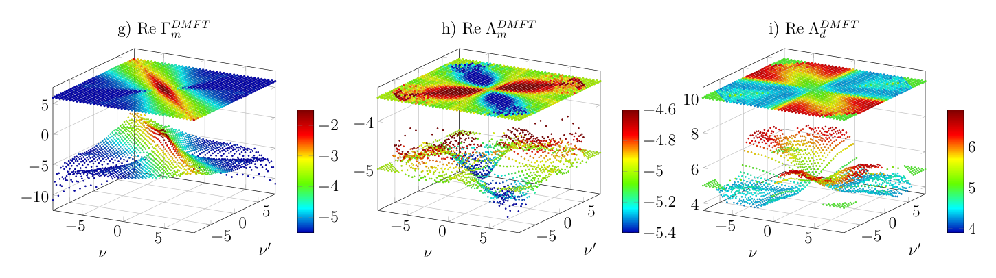
Fig. 6(a-c) shows, analogously to Fig. 5, the fermionic frequency dependence of the real part of the irreducible vertices in the magnetic and channels from the PA, but now for the filling of , comparing PA, DA and the local DMFT vertices. As already indicated by the eigenvalues, for this filling the magnetic vertex is slightly smaller at than for and as a result, at and is significantly smaller. Note that tiny differences in the eigenvalues that are close to one reflect large differences in the respective vertices themselves. In case of , it is the value of which is larger (Fig. 6c).
In Fig. 6(d-f) the respective DA results for the dynamical structure of the vertices are shown. The overall structure is identical to the PA. The magnitude of at and at and is however smaller; particularly in the case of . This is also reflected in the comparison between PA and DA eigenvalues shown in Fig. 3. The vertex at and is not much smaller in DA than in PA.
In Fig. 6(h-i) the real part of the DMFT fully irreducible vertex used as input to the parquet equations in DA is shown. For comparison, also the local DMFT vertex is shown (Fig. 6 g).
IV.4 Eigenvectors: -wave pairing
As already mentioned in Sec. III.4 the analysis of the symmetries of the eigenvectors corresponding to the largest eigenvalues allows us to predict the symmetry of the order parameter once the eigenvalue as a function of temperature crosses one and the respective susceptibility diverges. In the following, we hence study the symmetry of the eigenvector that corresponds to the largest eigenvalue in Eq. (8b), which presumably diverges at lower temperatures. We start the analysis by presenting the DA results for the filling of . As expected for this doping Bulut 2002; Maier et al. 2006, here the symmetry of the dominant eigenvector is—as we will see—-wave. The results obtained in the PA are qualitatively the same.
In Fig. 7 the momentum dependence of the dominant eigenvector for the first Matsubara frequency is shown (left-middle column) for the two cluster sizes and at , . For both cluster sizes the pattern is the same: we observe a sign change of the eigenvector (the predicted order parameter) as we move along the Fermi surface ( projected on the Fermi surface is shown in the right-middle column) with nodes at visible for the cluster. For the cluster we see only the sign change, as there are no points that would lie on the Fermi surface for this grid. The sign change of together with the fact that it is from the singlet channel shows that this eigenvalue is of -symmetry (the dominant contribution to is proportional to ). Hence, we have already labeled it correspondingly in Fig. 7.
In the right column of Fig. 7, the Fourier transform of from the left-middle column into real space is shown, i.e. , where measures the distance to surrounding sites in units of the lattice constant. We observe that the eigenvector is strongly peaked at the positions of nearest neighbors and changes sign depending on direction, which is in accordance with expectations for the -symmetry.
IV.4.1 Relation to magnetic susceptibility
In the left column of Fig. 7, the -dependence of the corresponding magnetic susceptibility is shown. It is peaked at . This magnetic ordering vector connects those points on the Fermi surface, where the eigenvector in the middle column of Fig. 7 is largest and has opposite sign, i.e., and and (cubic-)symmetrically related ones. It is the that to a large extent determines the sign pattern in momentum of the superconducting order parameter. This is seen from the Eliashberg Eq. (9): For repulsive interaction (), there has to be a sign change of the order parameter between the points and connected by . Please recall that our effective interaction, or pairing glue, is given by the irreducible vertex in the particle-particle channel, . This in turn, is essentially given by the magnetic susceptibility at since it is the largest particle-particle irreducible contribution.
IV.4.2 The particle-particle vertex in momentum and real space
In Fig. 8 we show the momentum (upper row) and real space (lower row) dependence of the irreducible vertex for obtained on a grid and two different values of in DA and PA. It is shown for the bosonic (transfer) momentum of and the lowest Matsubara frequencies, where the contribution is the biggest. The irreducible vertex can be interpreted as an effective interaction between electrons that enters the Eliashberg Eq. (9). In the momentum space the vertex is strongly peaked at , which is also the maximum of the magnetic susceptibility. The Fourier transform into real space (lower row of Fig. 8) corresponds to an attraction between electrons on neighboring sites, typical for the -wave symmetry. The full pattern in the real space of the vertex is the same in the PA and DA and in agreement with the one obtained in DCA. Scalapino 2012. There is a strong attractive (negative) interaction between nearest neighbors as well as strong repulsive (positive) interaction on-site and between second-nearest neighbors (see Fig. 8).
For the momentum and real-space dependence of is not only qualitatively but also quantitatively almost the same in DA and PA (cf. left and middle column of Fig. 8). In DA the magnitude of the nearest-neighbor attraction is slightly lower, which is also reflected in the -wave eigenvalue being smaller (cf. Fig. 3). This leads us again to a conclusion that for this value of , there is overall agreement between the PA and DA, and including the fully irreducible vertex dynamics leads only to a slight suppression of fluctuations.
For we present only the PA result (right column of Fig. 8) since as discussed earlier, no convergent DA results in this case are available at the moment. Although the temperature is slightly higher than in the case ( vs. ), the vertex is significantly larger and the effective attraction between nearest neighbors almost three times stronger. The overall structure in momentum and real space is however the same as in the case of .
IV.5 Eigenvectors: triplet -wave pairing
For higher dopings, the dominant eigenvalue corresponds to a different eigenvector, with a triplet spin symmetry. As for the case of the -wave symmetry in Sec. IV.4, we present in Fig. 9 the dominant eigenvector in momentum space (left-middle column) together with its projection on the Fermi surface (right-middle column), its Fourier transform into real space (right column) and the respective magnetic susceptibility (left column) from PA (upper row) and DA (middle row) at , and for the cluster. For DA we also present data for the same parameters but for the cluster. At the specific filling of , in DA the triplet -wave eigenvector corresponds to the biggest eigenvalue in the channel, whereas in the PA this is the second biggest eigenvalue with the -wave being still the largest one (cf. Fig 3). As we have discussed in Sec. IV.4, the -dependence of the susceptibility can help us build an intuitive picture. For both DA and PA the magnetic susceptibility is strongly peaked at the incommensurate wave vector (with dependent on the momentum grid used for the calculation). The value at is however still quite large in the case of PA, whereas for DA it is much smaller (cf. left column of Fig. 9). The antiferromagnetic fluctuations in PA are thus still strong enough to make -wave symmetry in the channel the dominant one, whereas in DA, triplet -wave pairing fluctuations already prevail.
Let us focus now on the triplet -wave eigenvector. Although the projection on the Fermi surface of the eigenvector (right-middle column of Fig. 9) is very similar in all the three cases shown, the momentum structure and therefore also the real space structure of the eigenvector is slightly different between PA and DA. Both are -wave (there are no sign changes for the neighbors equally distant from center), but the eigenvector turns negative for the second-nearest neighbors in PA, whereas it stays positive for both cluster sizes in DA.
IV.5.1 Relation to magnetic susceptibility
Looking at the peak in magnetic susceptibility at (shown in the left column of Fig. 9) and performing the same analysis as was done in Sec. IV.4 for the possible symmetry of the order parameter, we could conclude that the dominant eigenvector should look differently. In particular we could expect sign changes between the points on the Fermi surface connected by the now incommensurate wave vector of the (maximal) magnetic susceptibility. Since with an incommensurate there are 4 maxima in the susceptibility in the first Brillouin zone, there would have to be many sign changes of the order parameter on the Fermi surface. Such eigenvector is possible, but we found that the corresponding eigenvalue is significantly smaller than the triplet -wave one. Physically many sign changes would mean many zeroes of the order parameter on the Fermi surface, which is energetically not favorable. The -wave, with no sign changes, seems to be more favorable, although it does not take advantage specifically from the strong peak in the magnetic susceptibility at but rather from the -averaged value. This can be seen from Eliashberg Eq. (9): if we approximate the pairing vertex by a product of a frequency dependent part and momentum dependent part, the -wave order parameter without sign changes will pick up the momentum averaged vertex. Similar analysis how the momentum structure and/or frequency structure of the vertex in Eliashberg or eigenvalue equation influences the resulting order parameter can be found in Refs. Vojta and Dagotto 1999; Shigeta et al. 2009; Kitatani et al. 2017
IV.5.2 Importance of the frequency structure of the vertex
In the case where momentum structure cannot be used advantageously enough as explained in the previous paragraph, another factor plays an important role, namely the fermionic frequency dependence of the vertex. As can be seen in Fig. 6, (b-c) for the PA and (e-f) for the DA, the vertex is the strongest on the antidiagonal and it increases for larger frequencies. As we will see below, it is this structure that is advantageous for the odd-frequency pairing. With the order parameter in the Eliashberg Eq. (9) going to zero at (necessary in case of -wave triplet pairing) and changing sign, these strong contributions at finite frequencies can be picked up.
Odd-frequency, -wave pairing has, to the best of our knowledge, not been seen before to be the dominant eigenvalue in the 2D Hubbard model without frustration, but it has been reported for more exotic Hamiltonians Yada et al. 2008; Shigeta et al. 2009; Shigeta et al. 2012; Linder and Balatsky 2019. Let us emphasize, however, that the methods mainly used in this parameter regime (FLEX, RPA) do not fully consider the fermionic frequency dependence of the vertex.
To check the importance of this frequency dependence, we have used the eigenvalue equation (8b) to generate eigenvalues and eigenvectors from an interpolative vertex defined as
| (10) |
where , is the vertex at the first Matsubara frequencies and . This way, we interpolate between a frequency independent vertex (within the four quadrants given by the sign of and ) which has the same momentum structure () and the full vertex (). Since we are interested in the effect of the fermionic frequency dependence in the vertex, we have considered here only the eigenvalues for the case and and used the DA Green’s functions in Eq. (8b).
In Fig. 10 we show the fermionic frequency dependence of for the slice (on the antidiagonal) and for different values of for one specific momentum point , . Specifically, we have used the DA vertex Fig. 6 (e-f) for which the ratio between the triplet -wave eigenvalue to the one is and flattened the frequency dependence by reducing in Eq. (IV.5.2), see Fig. 10. As we see from the legend of Fig. 10, the ratio decreases when the frequency structure is flattened, down to for . That is, without the frequency dependence of the vertex, -wave symmetry (singlet, even-frequency) should dominate for this filling, which complies with the RPA results Rømer et al. 2015.
Note that the values of and obtained from Eq. (8b) with the interpolative vertex for different values of cannot be directly compared since the interpolative vertex is not an actual solution of the problem in any specific approximation. The above analysis nonetheless indicates that it is the fermionic frequency dependence of the vertex which is important for making odd-frequency -wave pairing the dominant superconducting fluctuation. The odd-frequency -wave competes with -wave even without imposing a strong frustration.
IV.5.3 The particle-particle vertex in momentum and real space
The particle-particle irreducible vertex for , and together with its Fourier transform into real space are shown in Fig. 11 for PA and in Fig. 12 for DA for the cluster. In the three columns of both figures we show the vertex (left column) and the singlet (middle column) and triplet (right column) contributions. The upper row shows the vertices in momentum space and the lower row their Fourier transform into real space, with the center denoting the on-site (local) contribution.
Let us first focus on the left column, i.e. . The momentum dependence in both PA and DA (upper left plot in Figs. 11 and 12) is peaked at and the three other symmetry related points, which shows again a clear relation between and the magnetic susceptibility . In PA the value at is almost as large as at and the structure of the vertex in real space (lower left plot in Fig. 11) resembles the typical one for -wave pairing symmetry, i.e., nearest-neighbor attraction and second-nearest-neighbor repulsion. Qualitatively the same nearest-neighbor attraction and second-nearest-neighbor repulsion is found for the clear-cut -wave case in Fig. 8 (all lower panels). Quantitatively, this second-nearest-neighbor repulsion is however very weak. That is, although the dominant eigenvalue for in PA corresponds to -wave symmetry (cf. Fig. 3), the influence of the second largest eigenvalue (-wave) is already visible.
In DA for the same , on the other hand, the vertex is not any more large at and the real space structure shown in lower left plot of Fig. 12 differs from the one in PA: The nearest-neighbor attraction is now much weaker and there is an attraction instead of repulsion for the second-nearest neighbors (the vertex is slightly negative also for the third and fourth layer of neighbors). The influence of the -wave contribution is clearly visible. It is also reflected in the -wave eigenvalue being bigger than -wave (cf. Fig. 3).
Next, let us look at the singlet vs. triplet contributions shown in middle and right column of Figs. 11 and 12. For both PA and DA, the nearest-neighbor attraction is present in the singlet channel, although much weaker in DA, whereas all further neighbor attraction is entirely in the triplet channel. The negative value of the singlet vertex for the furthest possible neighbors on the diagonal (both in PA and DA) could either be a higher order -wave contribution, which would be consistent with the incommensurate magnetic ordering vector, or a finite size effect which we cannot eliminate at the moment. This slight furthest neighbor attraction in the singlet channel is also present in the cluster calculations for large dopings (not shown here).
IV.6 Comparison with ladder-DA
In the following we compare the parquet DA results with the results obtained within the -corrected ladder DA method, as described in Ref. Kitatani et al. 2019. In the ladder method the vertices are calculated from vertices which in turn are obtained from a Bethe-Salpeter ladder built in the channel (starting from a purely local and ).foo c Additionally, in the calculation of susceptibilities and ladder vertices a Moriasque -correction Katanin et al. 2009; Rohringer et al. 2018 is made, which imitates the influence of insertions of -diagrams that are not present in the ladder. Therefore, the ladder method does not treat the and channels on equal footing. The advantage of ladder DA lies in the much larger cluster sizes that it can handle, since the ladder calculations involve only one momentum (contrary to the three needed in the parquet approach).
In Fig. 13 the comparison of magnetic and eigenvalues (top) and the momentum dependence of static magnetic susceptibilities (bottom) between ladder (denoted as ’ladder’) and parquet (denoted as in the rest of the paper ’DA’) versions of DA is shown. The results are compared for the two different fillings ( and ), and . For larger doping the difference between the results of the two methods is small and both the eigenvalues and magnetic susceptibility are similar. The eigenvalues are slightly larger in the ladder approximation and also the irreducible vertices shown in Fig. 14 (top two panels) are slightly larger.
In the case of there is a large difference both in -wave eigenvalue and in the susceptibility. There are two reasons for the differences: (i) the insertions from the channel are important and are not correctly reproduced by using the -correction and (ii) finite size effects are large, since the ladder calculation is converged in momentum grid and the parquet one used here is on the cluster.
In order to get some insight which of the effects dominates we have calculated the ladder DA magnetic susceptibility on a cluster (shown in Fig. 13 as the light blue for and pink for ). For the difference is quite dramatic, since on the cluster the incommensurate peak in the susceptibility is missing and its weight is distributed between the and points. That could explain the large difference of the -wave eigenvalues in the two methods and supports the (ii) explanation for the difference in the two methods. At higher temperatures, when the momentum resolution is less important, the eigenvalues lie closer to each other as can be seen in the upper panel of Fig. 4.
The vertices obtained in the two methods for the same parameters as above, shown in Fig. 14 also look similar, even for the filling of , which lets us conclude that the -correction in the ladder method fairly well reproduces the influence of diagrams in the channel for these parameters. Instead it is the finite grid which, for particular dopings, might miss the proper incommensurate wave vector.

In Fig. 15 the results analogous to those in Fig. 13 are shown for , and only one filling of . The ladder eigenvalues also show the triplet -wave as the dominant symmetry in the channel and they are both bigger than the parquet eigenvalues. Here the reasoning that eigenvalues could be smaller in the parquet DA due to missing of a strong peak in the magnetic channel is not valid, mainly because the peak is not so pronounced and also for odd frequency -wave pairing the momentum dependence is not that important as the frequency dependence as explained in Sec. IV.5.2. Looking at the frequency dependence of the vertices in both methods shown in Fig. 16 we see that the vertices in the ladder method are much stronger than in parquet DA, which leads to larger eigenvalues. Also the frequency dependence of the ladder vertices is steeper which leads to a larger ratio of the eigenvalues, compliant with the discussion in Sec. IV.5.2.

V Conclusion
We have performed a parquet equations study of the doped two dimensional Hubbard model using two different approximations for the fully irreducible vertex: the PA and parquet DA. In contrast to previous diagrammatic extensions of DMFT,Otsuki et al. 2014; Kitatani et al. 2019; Vučičević et al. 2017; Rohringer et al. 2018 we employ the parquet equations instead of using ladder diagrams for generating non-local correlations. Hence our approach is not biased against a certain scattering channel. All relevant fluctuations for unconventional superconductors, i.e. magnetic, superconducting, charge density wave fluctuations, are treated on an equal footing. This is particularly important since several instabilities are at close quarters and mutually influence each other: commensurate and incommensurate antiferromagnetism, singlet -wave and triplet -wave pairing.
Close to half-filling, we find predominant commensurate antiferromagnetic fluctuations at wave vector , and the leading fluctuation in the pairing channel are -wave. At finite but small dopings, e.g., at 15% doping or electrons per site, the -wave eigenvalue increases much faster upon lowering temperature than the antiferromagnetic one which even decreases at the lowest temperature accessible [Fig. 4 (top)]. Although we cannot exclude that another instability will start dominating at even lower temperatures, it is likely that for this doping -wave superconductivity eventually prevails, however with a smaller than many other methods predict. Kyung et al. 2003; Hafermann et al. 2008; Gull et al. 2013; Otsuki et al. 2014; Kitatani et al. 2015 From the structure of the eigenvalue (see below) and also from the fact that commensurate antiferromagnetic and -wave superconducting fluctuations show the same trends, e.g., they fall off concomitantly if we move toward higher doping [Fig. 3], we conclude that -wave pairing fluctuations are induced by (nearly) commensurate antiferromagnetic spin fluctuations. Let us also emphasize in this context that in the temperature and doping range studied we do not find charge density wave fluctuations with magnitude comparable to the magnetic ones.
At larger doping, we change from commensurate to highly incommensurate antiferromagnetic spin fluctuations with e.g. , and from singlet -wave to triplet -wave fluctuations in the pairing channel. Both eigenvalues, incommensurate antiferromagnetic and -wave pairing, show a similar doping dependence [Fig. 3].
If we connect points of the Fermi surface by the commensurate antiferromagnetic wave vector , it becomes clear that commensurate antiferromagnetic and -wave fluctuations match perfectly. The latter has a sign change for those points of the Fermi surface connected by , see Fig. 7. For incommensurate antiferromagnetism, there are now however four equivalent incommensurate wave vectors within the Brillouin zone [, , , , see Fig. 9]. A similar line of reasoning as for the commensurate wave vector would hence require many changes of sign on the Fermi surface. Such a complicated superconducting order parameter is conceivable, and a possible solution in our PA or parquet DA calculation. Indeed we find it to be the second largest pairing eigenvalue at large doping; the largest one is however a triplet -wave eigenvalue [shown in Fig. 9]. In the case of triplet odd-frequency -wave pairing, the order parameter does not specificaly profit from a pronounced peak at incommensurate , but rather from a -averaged value. Another factor which makes the odd-frequency -wave pairing fluctuations dominate over even in frequency -wave is the strong frequency structure of the vertex which is suppressed at small fermionic frequencies and away from the line with fermionic frequencies .
Our detailed analysis in real and -space does not only help us to unambiguously identify the eigenvalues in the pairing channel, but it also reveals the evolution from - to -wave. In real space, the superconducting pairing glue always has a strong local repulsion, reflecting the repulsive of the Hubbard model. For small dopings the antiferromagnetic spin-fluctuations provide however a substantial nearest-neighbor attraction along with second-nearest-neighbor repulsion [Fig. 8 (left)]. This eventually leads to a strong nearest-neighbor component of the -wave eigenvalue with the typical sign change in real space [Fig. 7 (right)]. For larger dopings this nearest-neighbor attraction gets weaker and the second-nearest-neighbor repulsion eventually becomes attractive [Fig. 12 (bottom left)]. Here, the -wave eigenvalue becomes favorable in DA, which has again a strong nearest-neighbor component but now without sign changes [Fig. 9 (lower and middle right)].
To sum up, our new development of the parquet equations solver enables us to analyze low-temperature physics of the doped Hubbard model and visualize all possible fluctuations in an unsupervised manner. We obtained that for smaller doping levels commensurate antiferromagnetic fluctuations lead to strong -wave pairing fluctuations, which become weaker as the doping is increased. For larger doping levels, we also observed that the triplet -wave odd-frequency pairing fluctuations become comparable (or even dominate) and we raised the frequency structure of the vertex as a new (but general) factor for supporting this observation. Since the temperature is still not low enough for discussing phase transitions, our unbiased study will provide useful insight for future studies on magnetism and superconductivity.
Acknowledgements
We thank J. Kuneš, P. Pudleiner, and T. Ribic for very helpful and inspiring discussions and C. Watzenböck for obtaining some of the DA input. The help of the Vienna Scientific Cluster (VSC) Team, in particular of C. Blaas-Schenner, in optimizing the code is also greatly acknowledged. The present work was supported financially by European Research Council under the European Union’s Seventh Framework Program (FP/2007-2013) through ERC Grant No. 306447 and the Austrian Science Fund (FWF) through SFB ViCoM F41 and project P 30997. G.L. acknowledges the starting grant of ShanghaiTech University, the Program for Professor of Special Appointment (Shanghai Eastern Scholar) and the support from the National Natural Science Foundation of China (Grant No. 11874263). Calculations have been done on the VSC.
Appendix A Convergence of the eigenvalues with respect to the number of frequencies
The parquet equations solver scales with the power of 3.4 in the number of frequencies and momenta used (stemming from one prefactor [power 1] in the number of frequencies/momenta and from a matrix-matrix multiplication [power 2.4]; using the point group symmetry reduces only the prefactor of this scaling). The victory code actual efficiency is however memory bound (see Ref. Li et al. 2019). For the momentum cluster most of the calculations were done for 64 frequencies (32 positive and 32 negative) and it was not possible to use more frequencies. At the lowest temperatures presented for the cluster ( for shown in Fig. 4, as well as for and for in Figs. 9 and 7) we were not able to obtain convergent results for a smaller number of frequencies. Therefore, cluster results at these temperatures are not converged with respect to the number of frequencies. Convergence analysis was done for the case, however. The frequency-box-size dependence of the eiganvalues for , is shown in Fig 17. Since the values do not change significantly between the box of 128 frequencies and the largest box taken (160 frequencies), most of the results presented in this paper were obtained using 128 frequencies. For higher temperatures, the results do not change already for 64 frequencies. Based on the results for the cluster, we can expect some quantitative differences in the eigenvalues for the cluster if we take a larger frequency box. However, we do not expect a qualitative change of the overall behavior.
References
- Bednorz and Müller (1986) J. G. Bednorz and K. A. Müller, Zeitschrift für Physik B Condensed Matter 64, 189 (1986).
- Dagotto (1994) E. Dagotto, Rev. Mod. Phys. 66, 763 (1994).
- Maeno et al. (1994) Y. Maeno, H. Hashimoto, K. Yoshida, S. Nishizaki, T. Fujita, J. G. Bednorz, and F. Lichtenberg, Nature 372, 532 (1994).
- Mackenzie and Maeno (2003) A. P. Mackenzie and Y. Maeno, Rev. Mod. Phys. 75, 657 (2003).
- Kamihara et al. (2006) Y. Kamihara, H. Hiramatsu, M. Hirano, R. Kawamura, H. Yanagi, T. Kamiya, and H. Hosono, J. Am. Chem. Soc. 128, 10012–10013 (2006).
- Wang et al. (2008) C. Wang, L. Li, S. Chi, Z. Zhu, Z. Ren, Y. Li, Y. Wang, X. Lin, Y. Luo, S. Jiang, X. Xu, G. Cao, and Z. Xu, EPL (Europhysics Letters) 83, 67006 (2008).
- Wollman et al. (1993) D. A. Wollman, D. J. Van Harlingen, W. C. Lee, D. M. Ginsberg, and A. J. Leggett, Phys. Rev. Lett. 71, 2134 (1993).
- Shen et al. (1993) Z.-X. Shen, D. S. Dessau, B. O. Wells, D. M. King, W. E. Spicer, A. J. Arko, D. Marshall, L. W. Lombardo, A. Kapitulnik, P. Dickinson, S. Doniach, J. DiCarlo, T. Loeser, and C. H. Park, Phys. Rev. Lett. 70, 1553 (1993).
- Tsuei et al. (1994) C. C. Tsuei, J. R. Kirtley, C. C. Chi, L. S. Yu-Jahnes, A. Gupta, T. Shaw, J. Z. Sun, and M. B. Ketchen, Phys. Rev. Lett. 73, 593 (1994).
- Maki (1998) K. Maki, AIP Conference Proceedings 438, 83 (1998), https://aip.scitation.org/doi/pdf/10.1063/1.56343 .
- Sigrist et al. (1999) M. Sigrist, D. Agterberg, A. Furusaki, C. Honerkamp, K. Ng, T. Rice, and M. Zhitomirsky, Physica C: Superconductivity 317-318, 134 (1999).
- Mazin et al. (2008) I. I. Mazin, D. J. Singh, M. D. Johannes, and M. H. Du, Phys. Rev. Lett. 101, 057003 (2008).
- Kuroki et al. (2008) K. Kuroki, S. Onari, R. Arita, H. Usui, Y. Tanaka, H. Kontani, and H. Aoki, Phys. Rev. Lett. 101, 087004 (2008).
- Ikeda et al. (2010) H. Ikeda, R. Arita, and J. Kuneš, Phys. Rev. B 81, 054502 (2010).
- Hanaguri et al. (2010) T. Hanaguri, S. Niitaka, K. Kuroki, and H. Takagi, Science 328, 474 (2010), http://science.sciencemag.org/content/328/5977/474.full.pdf .
- Hirschfeld et al. (2011) P. J. Hirschfeld, M. M. Korshunov, and I. I. Mazin, Reports on Progress in Physics 74, 124508 (2011).
- Kalenyuk et al. (2018) A. A. Kalenyuk, A. Pagliero, E. A. Borodianskyi, A. A. Kordyuk, and V. M. Krasnov, Phys. Rev. Lett. 120, 067001 (2018).
- Scalapino (2012) D. J. Scalapino, Rev. Mod. Phys. 84, 1383 (2012).
- White et al. (1989a) S. R. White, D. J. Scalapino, R. L. Sugar, E. Y. Loh, J. E. Gubernatis, and R. T. Scalettar, Phys. Rev. B 40, 506 (1989a).
- White et al. (1989b) S. R. White, D. J. Scalapino, R. L. Sugar, N. E. Bickers, and R. T. Scalettar, Phys. Rev. B 39, 839 (1989b).
- Bulut et al. (1993) N. Bulut, D. J. Scalapino, and S. R. White, Phys. Rev. B 47, 6157 (1993).
- Scalapino (1999) D. Scalapino, Journal of Low Temperature Physics 117, 179 (1999).
- Bulut (2002) N. Bulut, Adv. Phys. 51, 1587 (2002).
- Zanchi and Schulz (1998) D. Zanchi and H. J. Schulz, EPL (Europhysics Letters) 44, 235 (1998).
- Halboth and Metzner (2000a) C. J. Halboth and W. Metzner, Phys. Rev. B 61, 7364 (2000a).
- Halboth and Metzner (2000b) C. J. Halboth and W. Metzner, Phys. Rev. Lett. 85, 5162 (2000b).
- Honerkamp (2001) C. Honerkamp, The European Physical Journal B - Condensed Matter and Complex Systems 21, 81 (2001).
- Honerkamp et al. (2001) C. Honerkamp, M. Salmhofer, N. Furukawa, and T. M. Rice, Phys. Rev. B 63, 035109 (2001).
- Metzner et al. (2012) W. Metzner, M. Salmhofer, C. Honerkamp, V. Meden, and K. Schönhammer, Rev. Mod. Phys. 84, 299 (2012).
- Bickers et al. (1989) N. E. Bickers, D. J. Scalapino, and S. R. White, Phys. Rev. Lett. 62, 961 (1989).
- Moriya et al. (1990) T. Moriya, Y. Takahashi, and K. Ueda, Journal of the Physical Society of Japan 59, 2905 (1990), https://doi.org/10.1143/JPSJ.59.2905 .
- Manske (2004) D. Manske, Theory of Unconventional Superconductors (Springer, Berlin Heidelberg, 2004).
- Hanke et al. (2006) W. Hanke, M. Aichhorn, E. Arrigoni, and M. Potthoff, Physica B: Condensed Matter 378-380, 60 (2006), proceedings of the International Conference on Strongly Correlated Electron Systems.
- Kyung et al. (2003) B. Kyung, J.-S. Landry, and A.-M. S. Tremblay, Phys. Rev. B 68, 174502 (2003).
- Lichtenstein and Katsnelson (2000) A. I. Lichtenstein and M. I. Katsnelson, Phys. Rev. B 62, R9283 (2000).
- Maier et al. (2005a) T. Maier, M. Jarrell, T. Pruschke, and M. H. Hettler, Rev. Mod. Phys. 77, 1027 (2005a).
- Maier et al. (2005b) T. A. Maier, M. Jarrell, T. C. Schulthess, P. R. C. Kent, and J. B. White, Phys. Rev. Lett. 95, 237001 (2005b).
- Capone and Kotliar (2006) M. Capone and G. Kotliar, Phys. Rev. B 74, 054513 (2006).
- Haule and Kotliar (2007) K. Haule and G. Kotliar, Phys. Rev. B 76, 104509 (2007).
- Sordi et al. (2012) G. Sordi, P. Sémon, K. Haule, and A.-M. S. Tremblay, Phys. Rev. Lett. 108, 216401 (2012).
- Gull et al. (2013) E. Gull, O. Parcollet, and A. J. Millis, Phys. Rev. Lett. 110, 216405 (2013).
- Toschi et al. (2007) A. Toschi, A. A. Katanin, and K. Held, Phys Rev. B 75, 045118 (2007).
- Rubtsov et al. (2009) A. N. Rubtsov, M. I. Katsnelson, A. I. Lichtenstein, and A. Georges, Phys. Rev. B 79, 045133 (2009).
- Katanin et al. (2009) A. A. Katanin, A. Toschi, and K. Held, Phys. Rev. B 80, 075104 (2009).
- Hafermann et al. (2009) H. Hafermann, M. Kecker, S. Brener, A. N. Rubtsov, M. I. Katsnelson, and A. I. Lichtenstein, J Supercond Nov Magn 22, 45 (2009).
- Otsuki et al. (2014) J. Otsuki, H. Hafermann, and A. I. Lichtenstein, Phys. Rev. B 90, 235132 (2014).
- Taranto et al. (2014) C. Taranto, S. Andergassen, J. Bauer, K. Held, A. Katanin, W. Metzner, G. Rohringer, and A. Toschi, Phys. Rev. Lett. 112, 196402 (2014).
- Kitatani et al. (2015) M. Kitatani, N. Tsuji, and H. Aoki, Phys. Rev. B 92, 085104 (2015).
- Kitatani et al. (2017) M. Kitatani, N. Tsuji, and H. Aoki, Phys. Rev. B 95, 075109 (2017).
- Ayral and Parcollet (2015) T. Ayral and O. Parcollet, Phys Rev. B 92, 115109 (2015).
- Gukelberger et al. (2017) J. Gukelberger, E. Kozik, and H. Hafermann, Phys. Rev. B 96, 035152 (2017).
- Vučičević et al. (2017) J. Vučičević, T. Ayral, and O. Parcollet, Phys. Rev. B 96, 104504 (2017).
- Kitatani et al. (2019) M. Kitatani, T. Schäfer, H. Aoki, and K. Held, Phys. Rev. B 99, 041115 (2019).
- Rohringer et al. (2018) G. Rohringer, H. Hafermann, A. Toschi, A. A. Katanin, A. E. Antipov, M. I. Katsnelson, A. I. Lichtenstein, A. N. Rubtsov, and K. Held, Rev. Mod. Phys. 90, 025003 (2018).
- Aligia et al. (1998) E. Aligia, A.A.and Gagliano, L. Arrachea, and K. Hallberg, Euro. Phys. J. B 5, 371 (1998).
- Rømer et al. (2015) A. T. Rømer, A. Kreisel, I. Eremin, M. A. Malakhov, T. A. Maier, P. J. Hirschfeld, and B. M. Andersen, Phys. Rev. B 92, 104505 (2015).
- Diatlov et al. (1957) I. T. Diatlov, V. V. Sudakov, and K. A. Ter-Martirosian, Sov. Phys. JETP 5, 631 (1957).
- De Dominicis (1962) C. De Dominicis, J. Math. Phys. 3, 983 (1962).
- De Dominicis and Martin (1964) C. De Dominicis and P. C. Martin, J. Math. Phys. 5, 14 (1964).
- Valli et al. (2015) A. Valli, T. Schäfer, P. Thunström, G. Rohringer, S. Andergassen, G. Sangiovanni, K. Held, and A. Toschi, Phys. Rev. B 91, 115115 (2015).
- Li et al. (2016) G. Li, N. Wentzell, P. Pudleiner, P. Thunström, and K. Held, Phys. Rev. B 93, 165103 (2016).
- Pudleiner et al. (2019a) P. Pudleiner, P. Thunström, A. Valli, A. Kauch, G. Li, and K. Held, Phys. Rev. B 99, 125111 (2019a).
- Pudleiner et al. (2019b) P. Pudleiner, A. Kauch, K. Held, and G. Li, Phys. Rev. B 100, 075108 (2019b).
- Kauch et al. (2020) A. Kauch, P. Pudleiner, K. Astleithner, P. Thunström, T. Ribic, and K. Held, Phys. Rev. Lett. 124, 047401 (2020).
- Sayyad et al. (2020) S. Sayyad, E. W. Huang, M. Kitatani, M.-S. Vaezi, Z. Nussinov, A. Vaezi, and H. Aoki, Phys. Rev. B 101, 014501 (2020).
- Schulz (1990) H. J. Schulz, Phys. Rev. Lett. 64, 1445 (1990).
- Freericks and Jarrell (1995) J. K. Freericks and M. Jarrell, Phys. Rev. Lett. 74, 186 (1995).
- Tahvildar-Zadeh et al. (1997) A. N. Tahvildar-Zadeh, J. K. Freericks, and M. Jarrell, Phys. Rev. B 55, 942 (1997).
- Yamase et al. (2016) H. Yamase, A. Eberlein, and W. Metzner, Phys. Rev. Lett. 116, 096402 (2016).
- Schäfer et al. (2017) T. Schäfer, A. A. Katanin, K. Held, and A. Toschi, Phys. Rev. Lett. 119, 046402 (2017).
- Šimkovic et al. (2017) F. Šimkovic, Y. Deng, N. V. Prokof’ev, B. V. Svistunov, I. S. Tupitsyn, and E. Kozik, Phys. Rev. B 96, 081117 (2017).
- Linder and Balatsky (2019) J. Linder and A. V. Balatsky, Rev. Mod. Phys. 91, 045005 (2019).
- Vojta and Dagotto (1999) M. Vojta and E. Dagotto, Phys. Rev. B 59, R713 (1999).
- Yada et al. (2008) K. Yada, S. Onari, Y. Tanaka, and K. Miyake, arXiv e-prints , arXiv:0806.4241 (2008), arXiv:0806.4241 [cond-mat.supr-con] .
- Shigeta et al. (2009) K. Shigeta, S. Onari, K. Yada, and Y. Tanaka, Phys. Rev. B 79, 174507 (2009).
- Shigeta et al. (2012) K. Shigeta, S. Onari, and Y. Tanaka, Phys. Rev. B 85, 224509 (2012).
- Otsuki (2015) J. Otsuki, Phys. Rev. Lett. 115, 036404 (2015).
- Scalapino (2007) D. J. Scalapino, “Numerical studies of the 2d hubbard model,” in Handbook of High-Temperature Superconductivity: Theory and Experiment, edited by J. R. Schrieffer and J. S. Brooks (Springer New York, New York, NY, 2007) pp. 495–526.
- Li et al. (2019) G. Li, A. Kauch, P. Pudleiner, and K. Held, Computer Physics Communications 241, 146 (2019).
- Janiš (2001) V. Janiš, Phys. Rev. B 64, 115115 (2001).
- Janiš et al. (2017) V. Janiš, A. Kauch, and V. Pokorný, Phys. Rev. B 95, 045108 (2017).
- foo (a) (a), that is, cutting a Green’s function line does not separate the Feynman diagram into two pieces.
- Bickers (2004) N. Bickers, in Theoretical Methods for Strongly Correlated Electrons, CRM Series in Mathematical Physics, edited by D. Snchal, A.-M. Tremblay, and C. Bourbonnais (Springer New York, 2004) pp. 237–296.
- Rohringer et al. (2012) G. Rohringer, A. Valli, and A. Toschi, Phys. Rev. B 86, 125114 (2012).
- Parragh et al. (2012) N. Parragh, A. Toschi, K. Held, and G. Sangiovanni, Phys. Rev. B 86, 155158 (2012).
- Hörbinger (2018) F. Hörbinger, (2018), master Thesis.
- Chen et al. (2015) X. Chen, J. P. F. LeBlanc, and E. Gull, Phys. Rev. Lett. 115, 116402 (2015).
- Maier and Scalapino (2019) T. A. Maier and D. J. Scalapino, npj Quantum Materials 4, 30 (2019).
- foo (b) (b), for both and the temperature is the lowest for which we could converge the PA calculations at all fillings.
- Mermin and Wagner (1966) N. D. Mermin and H. Wagner, Phys. Rev. Lett. 17, 1307 (1966).
- Bickers and Scalapino (1992) N. E. Bickers and D. J. Scalapino, Phys. Rev. B 46, 8050 (1992).
- Maier et al. (2006) T. A. Maier, M. Jarrell, and D. J. Scalapino, Phys. Rev. B 74, 094513 (2006).
- foo (c) (c), please note, that the particle-particle vertices are symmetrized with respect to the outgoing fermionic lines in contrast to Ref. Kitatani et al. 2019.
- Hafermann et al. (2008) H. Hafermann, S. Brener, A. Rubtsov, M. Katsnelson, and A. Lichtenstein, JETP Letters 86, 677 (2008).