跳到论文正文
W Papers独立论文阅读器 arXiv:1901.09397 论文正文 计算阅读时间 · 0%
引用这篇论文根据当前论文元数据生成,正式投稿前建议核对。


License: arXiv.org perpetual non-exclusive license
arXiv:1901.09397v4 [math.AP] 29 Oct 2023

Analytic regularity for a singularly perturbed reaction-convection-diffusion boundary value problem with two small parameters

I. Sykopetritou    C. Xenophontos Note: Department of Mathematics and Statistics, University of Cyprus, PO BOX 20537, Nicosia 1678, Cyprus.
Abstract

We consider a second order, two-point, singularly perturbed boundary value problem, of reaction-convection-diffusion type with two small parameters, and we obtain analytic regularity results for its solution, under the assumption of analytic input data. First, we establish classical differentiability bounds that are explicit in the order of differentiation and the singular perturbation parameters. Next, for small values of these parameters we show that the solution can be decomposed into a smooth part, boundary layers at the two endpoints, and a negligible remainder. Derivative estimates are obtained for each component of the solution, which again are explicit in the differentiation order and the singular perturbation parameters.

1 Introduction

Singularly perturbed problems, and the numerical approximation of their solution, have been studied extensively over the last few decades (see, e.g., the books [9], [10], [13] and the references therein). As is well known, a main difficulty in these problems is the presence of boundary layers in the solution, which appear due to fact that the limiting problem (i.e. when the singular perturbation parameter(s) tend to 0), is of different order than the original one, and the (‘extra’) boundary conditions can only be satisfied if the solution varies rapidly in the vicinity of the boundary – hence the name boundary layers.

In most numerical methods, high order derivatives of the solution appear in the error estimates, hence one should have a clear picture of how these derivatives grow with respect to the singular perturbation parameter(s). For low order numerical methods, such as Finite Differences (FD) or the hh version of the Finite Element Method (FEM), derivatives up to order 3 are usually sufficient. For high order methods such as the h​php version of the FEM, derivatives of arbitrary order are needed, thus knowing how these behave with respect to the singular perturbation parameter(s) as well as the differentiation order, is necessary. Usually problems of convection-diffusion or reaction-diffusion type are studied separately and several researchers have proposed and analyzed numerical schemes for the robust approximation of their solution (see, e.g., [13] and the references therein). When there are two singular perturbation parameters present in the differential equation, the problem becomes reaction-convection-diffusion and the relationship between the parameters determines the ‘regime’ we are in (as shown in Table 1 ahead). In [3], the numerical solution to this problem was addressed, using the hh version of the FEM as well as appropriate finite differences (see also [1], [2], [4], [12], [14], [17], [18]). Our interest in is high order h​php FEM, hence we require information on all derivatives of the solution. In the present article we obtain information about the analytic regularity of the solution, using the method of asymptotic expansions (see also [5]), thus providing the tools for an h​php FEM for the approximation of such problems.

The rest of the paper is organized as follows: in Section 2 we present the model problem and the regularity of its solution in terms of classical differentiability. Section 3 contains the asymptotic expansion for the solution, under the assumption that the singular perturbation parameters are small enough. We consider all possible relationships between the singular perturbation parameters, and establish derivative bounds which are explicit in the differentiation order as well as the singular perturbation parameters. We also comment on the transition between the regimes, in the final subsection of Section 3. Finally, in Section 4 we summarize our conclusions.

With I⊂ℝI\subset\mathbb{R} an open, bounded interval with boundary ∂I\partial I and measure |I|\left|I\right|, we will denote by Ck​(I)C^{k}(I) the space of continuous functions on II with continuous derivatives up to order kk. We will use the usual Sobolev spaces Wk,m​(I)W^{k,m}(I) of functions on II with 0,1,2,…,k0,1,2,...,k generalized derivatives in Lm​(I)L^{m}\left(I\right), equipped with the norm and seminorm ‖⋅‖k,m,I\left\|\cdot\right\|_{k,m,I} and |⋅|k,m,I\left|\cdot\right|_{k,m,I}\,, respectively. When m=2m=2, we will write Hk​(I)H^{k}\left(I\right) instead of Wk,2​(I)W^{k,2}\left(I\right), and for the norm and seminorm, we will write ‖⋅‖k,I\left\|\cdot\right\|_{k,I} and |⋅|k,I\left|\cdot\right|_{k,I}\,, respectively. The usual L2​(I)L^{2}(I) inner product will be denoted by ⟨⋅,⋅⟩I\left\langle\cdot,\cdot\right\rangle_{I}, with the subscript omitted when there is no confusion. We will also use the space

H01​(I)={u∈H1​(I):u|∂I=0}.H_{0}^{1}\left(I\right)=\left\{u\in H^{1}\left(I\right):\left.u\right|_{\partial I}=0\right\}.

The norm of the space L∞​(I)L^{\infty}(I) of essentially bounded functions is denoted by ∥⋅∥∞,I\|\cdot\|_{\infty,I}. Finally, the notation “a≲ba\lesssim b” means “a≤C​ba\leq Cb” with CC being a generic positive constant, independent of any discretization or singular perturbation parameters.

2 The model problem and its regularity

We consider the following model problem (cf. [8]): Find uu such that

−ε1​u′′​(x)+ε2​b​(x)​u′​(x)+c⁡(x)​u​(x)\displaystyle-\varepsilon_{1}u^{\prime\prime}(x)+\varepsilon_{2}b(x)u^{\prime}(x)+c(x)u(x) =\displaystyle= f⁡(x),x∈I=(0,1),\displaystyle f(x)\;,\;x\in I=\left(0,1\right), (1)
u⁡(0)=u⁡(1)\displaystyle u(0)=u(1) =\displaystyle= 0 ,\displaystyle 0\text{ }, (2)

where 0<ε1,ε2≤10<\varepsilon_{1},\varepsilon_{2}\leq 1 are given parameters that can approach zero, and the functions b,c,fb,c,f are given and sufficiently smooth. In particular, we assume that they are analytic functions satisfying, for some positive constants γf,γc,γb\gamma_{f},\gamma_{c},\gamma_{b} independent of ε1,ε2,\varepsilon_{1},\varepsilon_{2},

‖f(n)‖∞,I≲n!γfn,‖c(n)‖∞,I≲n!γcn,‖b(n)‖∞,I≲n!γbn∀n=0,1,2,… .\left\|f^{(n)}\right\|_{\infty,I}\lesssim n!\gamma_{f}^{n}\;,\;\left\|c^{(n)}\right\|_{\infty,I}\lesssim n!\gamma_{c}^{n}\;,\;\left\|b^{(n)}\right\|_{\infty,I}\lesssim n!\gamma_{b}^{n}\;\;\forall\;n=0,1,2,...\text{ .} (3)

In addition, we assume that there exist constants β,γ,ρ\beta,\gamma,\rho, independent of ε1,ε2,\varepsilon_{1},\varepsilon_{2}, such that ∀x∈I¯=[0,1]\forall\;x\in\overline{I}=[0,1] there holds

b⁡(x)≥β>0,c⁡(x)≥γ>0,c⁡(x)−ε22​b′​(x)≥ρ>0.b(x)\geq\beta>0\;,\;c(x)\geq\gamma>0\;,\;c(x)-\frac{\varepsilon_{2}}{2}b^{\prime}(x)\geq\rho>0. (4)

The solution to (1), (2) satisfies (see, e.g. [3])

‖u‖∞,I≲1.\left\|u\right\|_{\infty,I}\lesssim 1. (5)

We would like to obtain a similar estimate for u′u^{\prime}. This is achieved in the following.

Lemma 1.

Let uu be the solution of (1), (2) and assume (3), (4) hold. Then

‖u′‖∞,I≲ε1−1.\left\|u^{\prime}\right\|_{\infty,I}\lesssim\varepsilon_{1}^{-1}.
Proof.

The proof follows [7]. Let

A⁡(x)=ε2ε1​∫x1b⁡(t)​𝑑t,A(x)=\frac{\varepsilon_{2}}{\varepsilon_{1}}\int_{x}^{1}b(t)dt,

and note that A⁡(1)=0A(1)=0 and A′​(x)=−ε2ε1​b​(x).A^{\prime}(x)=-\frac{\varepsilon_{2}}{\varepsilon_{1}}b(x). Then, multiplying (1) by eA⁡(x)e^{A(x)} and integrating from xx to 11, gives

−ε1​u′​(1)+ε1​eA⁡(x)​u′​(x)+∫x1eA⁡(t)​c​(t)​u​(t)​𝑑t=∫x1eA⁡(t)​f​(t)​𝑑t.-\varepsilon_{1}u^{\prime}(1)+\varepsilon_{1}e^{A(x)}u^{\prime}(x)+\int_{x}^{1}e^{A(t)}c(t)u(t)dt=\int_{x}^{1}e^{A(t)}f(t)dt.

Multiplying by ε1−1​e−A⁡(x)\varepsilon_{1}^{-1}e^{-A(x)} yields

u′​(x)=e−A⁡(x)​u′​(1)−1ε1​∫x1eA⁡(t)−A⁡(x)​c​(t)​u​(t)​𝑑t+1ε1​∫x1eA⁡(t)−A⁡(x)​f​(t)​𝑑t.u^{\prime}(x)=e^{-A(x)}u^{\prime}(1)-\frac{1}{\varepsilon_{1}}\int_{x}^{1}e^{A(t)-A(x)}c(t)u(t)dt+\frac{1}{\varepsilon_{1}}\int_{x}^{1}e^{A(t)-A(x)}f(t)dt. (6)

Integrating from 00 to 1,1, we further get

0=u′​(1)​∫01e−A⁡(x)​𝑑x−1ε1​∫01∫x1eA⁡(t)−A⁡(x)​[c⁡(t)​u​(t)−f⁡(t)]​𝑑t​𝑑x.0=u^{\prime}(1)\int_{0}^{1}e^{-A(x)}dx-\frac{1}{\varepsilon_{1}}\int_{0}^{1}\int_{x}^{1}e^{A(t)-A(x)}\left[c(t)u(t)-f(t)\right]dtdx. (7)

Since we wish to first estimate u′​(1)u^{\prime}(1), we need upper and lower bounds for ∫01e−A⁡(x)​𝑑x\int_{0}^{1}e^{-A(x)}dx. From (4) we have

∫01e−A⁡(x)​𝑑x≤∫01e−ε2ε1​β​(1−x)​𝑑x≤ε1ε2​β.\int_{0}^{1}e^{-A(x)}dx\leq\int_{0}^{1}e^{-\frac{\varepsilon_{2}}{\varepsilon_{1}}\beta(1-x)}dx\leq\frac{\varepsilon_{1}}{\varepsilon_{2}\beta}. (8)

Similarly,

∫01e−A⁡(x)​𝑑x≥∫01e−ε2ε1​‖b‖∞,I​(1−x)​𝑑x=ε1ε2​‖b‖∞,I​(1−e−ε2ε1​‖b‖∞,I).\int_{0}^{1}e^{-A(x)}dx\geq\int_{0}^{1}e^{-\frac{\varepsilon_{2}}{\varepsilon_{1}}\left\|b\right\|_{\infty,I}(1-x)}dx=\frac{\varepsilon_{1}}{\varepsilon_{2}\left\|b\right\|_{\infty,I}}\left(1-e^{-\frac{\varepsilon_{2}}{\varepsilon_{1}}\left\|b\right\|_{\infty,I}}\right). (9)

Also, to estimate the remaining terms in (7), we consider

1ε1​∫01∫x1eA⁡(t)−A⁡(x)​𝑑t​𝑑x=1ε1​∫01∫x1eA′​(ζ)​(t−x)​𝑑t​𝑑x,\frac{1}{\varepsilon_{1}}\int_{0}^{1}\int_{x}^{1}e^{A(t)-A(x)}dtdx=\frac{1}{\varepsilon_{1}}\int_{0}^{1}\int_{x}^{1}e^{A^{\prime}(\zeta)(t-x)}dtdx,

for some ζ\zeta between tt and xx. Hence,

1ε1​∫01∫x1eA⁡(t)−A⁡(x)​𝑑t​𝑑x≤1ε1​∫01∫x1e−ε2ε1​β​(t−x)​𝑑t​𝑑x≲1ε2+ε1ε22.\frac{1}{\varepsilon_{1}}\int_{0}^{1}\int_{x}^{1}e^{A(t)-A(x)}dtdx\leq\frac{1}{\varepsilon_{1}}\int_{0}^{1}\int_{x}^{1}e^{-\frac{\varepsilon_{2}}{\varepsilon_{1}}\beta(t-x)}dtdx\lesssim\frac{1}{\varepsilon_{2}}+\frac{\varepsilon_{1}}{\varepsilon_{2}^{2}}.

Using (7)–(9), we get

|u′​(1)|\displaystyle\left|u^{\prime}(1)\right| ≲\displaystyle\lesssim 1[∫01e−A⁡(x)​𝑑x]​[(‖c‖∞,I​‖u‖∞,I+‖f‖∞,I)​(1ε2+ε1ε22)]\displaystyle\frac{1}{\left[\int_{0}^{1}e^{-A(x)}dx\right]}\left[\left(\left\|c\right\|_{\infty,I}\left\|u\right\|_{\infty,I}+\left\|f\right\|_{\infty,I}\right)\left(\frac{1}{\varepsilon_{2}}+\frac{\varepsilon_{1}}{\varepsilon_{2}^{2}}\right)\right]
≲\displaystyle\lesssim ε2​‖b‖∞,Iε1​(1−e−ε2ε1​‖b‖∞,I)−1​(1ε2+ε1ε22)\displaystyle\varepsilon_{2}\frac{\left\|b\right\|_{\infty,I}}{\varepsilon_{1}}\left(1-e^{-\frac{\varepsilon_{2}}{\varepsilon_{1}}\left\|b\right\|_{\infty,I}}\right)^{-1}\left(\frac{1}{\varepsilon_{2}}+\frac{\varepsilon_{1}}{\varepsilon_{2}^{2}}\right)
≲\displaystyle\lesssim ε1−1.\displaystyle\varepsilon_{1}^{-1}.

Inserting this bound in (6) gives

|u′​(x)|\displaystyle\left|u^{\prime}(x)\right| ≲\displaystyle\lesssim ε1−1+1ε1​(‖c‖∞,I​‖u‖∞,I+‖f‖∞,I)​∫x1eA⁡(t)−A⁡(x)​𝑑t\displaystyle\varepsilon_{1}^{-1}+\frac{1}{\varepsilon_{1}}\left(\left\|c\right\|_{\infty,I}\left\|u\right\|_{\infty,I}+\left\|f\right\|_{\infty,I}\right)\int_{x}^{1}e^{A(t)-A(x)}dt
≲\displaystyle\lesssim ε1−1+1ε1​(‖c‖∞,I​‖u‖∞,I+‖f‖∞,I)​∫x1e−ε2ε1​β​(t−x)​𝑑t\displaystyle\varepsilon_{1}^{-1}+\frac{1}{\varepsilon_{1}}\left(\left\|c\right\|_{\infty,I}\left\|u\right\|_{\infty,I}+\left\|f\right\|_{\infty,I}\right)\int_{x}^{1}e^{-\frac{\varepsilon_{2}}{\varepsilon_{1}}\beta(t-x)}dt
≲\displaystyle\lesssim ε1−1+1ε1​(ε1ε2​β)\displaystyle\varepsilon_{1}^{-1}+\frac{1}{\varepsilon_{1}}\left(\frac{\varepsilon_{1}}{\varepsilon_{2}\beta}\right)
≲\displaystyle\lesssim ε1−1,\displaystyle\varepsilon_{1}^{-1},

as desired. ∎

Using an inductive argument we are able to prove the following.

Theorem 2.

Let uu be the solution of (1), (2), and assume ε1≤ε2\varepsilon_{1}\leq\varepsilon_{2}. Then, there exist positive constants C,KC,K, independent of ε1,ε2\varepsilon_{1},\varepsilon_{2} and uu, such that for n=0,1,2,…n=0,1,2,...

‖u(n)‖∞,I≤C​Kn​max⁡{n,ε1−1}n.\left\|u^{(n)}\right\|_{\infty,I}\leq CK^{n}\max\left\{n,\varepsilon_{1}^{-1}\right\}^{n}.
Proof.

The proof is by induction on nn and follows [5]. Equation (5) and Lemma 1 give the result for n=0,1n=0,1, so we assume it holds for 0≤ν≤n+10\leq\nu\leq n+1 and show that it holds for n+2n+2. Differentiating (1) nn times gives

−ε1​u(n+2)\displaystyle-\varepsilon_{1}u^{(n+2)} =\displaystyle= f(n)−ε2​(b​u′)(n)−(c​u)(n)\displaystyle f^{(n)}-\varepsilon_{2}\left(bu^{\prime}\right)^{(n)}-\left(cu\right)^{(n)}
=\displaystyle= f(n)−∑ν=0n(nν)⁡(ε2​b(ν)​u(n+1−ν)+c(ν)​u(n−ν)).\displaystyle f^{(n)}-\sum_{\nu=0}^{n}\binom{n}{\nu}\left(\varepsilon_{2}b^{(\nu)}u^{(n+1-\nu)}+c^{(\nu)}u^{(n-\nu)}\right).

By the induction hypothesis we have

ε1​‖u(n+2)‖∞,I\displaystyle\varepsilon_{1}\left\|u^{(n+2)}\right\|_{\infty,I} ≤\displaystyle\leq ‖f(n)‖∞,I+\displaystyle\left\|f^{(n)}\right\|_{\infty,I}+
+C∑ν=0n(nν)[ε2γbνν!Kn+1−νmax{n+1−ν,ε1−1}n+1−ν+\displaystyle+C\sum_{\nu=0}^{n}\binom{n}{\nu}\left[\varepsilon_{2}\gamma_{b}^{\nu}\nu!K^{n+1-\nu}\max\left\{n+1-\nu,\varepsilon_{1}^{-1}\right\}^{n+1-\nu}+\right.
+γcνν!Kn−νmax{n−ν,ε1−1}n−ν].\displaystyle\left.+\gamma_{c}^{\nu}\nu!K^{n-\nu}\max\left\{n-\nu,\varepsilon_{1}^{-1}\right\}^{n-\nu}\right].

Using the estimates below (which follow by standard considerations)

(nν)​ν!​max⁡{n+1−ν,ε1−1}n+1−ν≤max⁡{n+1,ε1−1}n+1,\binom{n}{\nu}\nu!\max\left\{n+1-\nu,\varepsilon_{1}^{-1}\right\}^{n+1-\nu}\leq\max\left\{n+1,\varepsilon_{1}^{-1}\right\}^{n+1},
(nν)​ν!​max⁡{n−ν,ε1−1}n−ν≤max⁡{n+1,ε1−1}n+1,\binom{n}{\nu}\nu!\max\left\{n-\nu,\varepsilon_{1}^{-1}\right\}^{n-\nu}\leq\max\left\{n+1,\varepsilon_{1}^{-1}\right\}^{n+1},
‖f(n)‖∞,I≤C​γfn​n!≤C​γfn​max⁡{n+1,ε1−1}n+1,\left\|f^{(n)}\right\|_{\infty,I}\leq C\gamma_{f}^{n}n!\leq C\gamma_{f}^{n}\max\left\{n+1,\varepsilon_{1}^{-1}\right\}^{n+1},

we obtain

ε1​‖u(n+2)‖∞,I≤C​γfn​max⁡{n+1,ε1−1}n+1+\varepsilon_{1}\left\|u^{(n+2)}\right\|_{\infty,I}\leq C\gamma_{f}^{n}\max\left\{n+1,\varepsilon_{1}^{-1}\right\}^{n+1}+
+CKn+2max{n+1,ε1−1}n+1∑ν=0n[1K(γbK)ν+1K2(γcK)ν]+CK^{n+2}\max\left\{n+1,\varepsilon_{1}^{-1}\right\}^{n+1}\sum_{\nu=0}^{n}\left[\frac{1}{K}\left(\frac{\gamma_{b}}{K}\right)^{\nu}+\frac{1}{K^{2}}\left(\frac{\gamma_{c}}{K}\right)^{\nu}\right]
≤C​Kn+2​max⁡{n+1,ε1−1}n+1​[1K2+1K​1(1−γb/K)+1K2​1(1−γc/K)],\leq CK^{n+2}\max\left\{n+1,\varepsilon_{1}^{-1}\right\}^{n+1}\left[\frac{1}{K^{2}}+\frac{1}{K}\frac{1}{(1-\gamma_{b}/K)}+\frac{1}{K^{2}}\frac{1}{(1-\gamma_{c}/K)}\right],

where we choose the constant K>max⁡{1,γf,γb,γc}K>\max\{1,\gamma_{f},\gamma_{b},\gamma_{c}\} such that the expression in brackets above is bounded by 1. Thus

ε1​‖u(n+2)‖∞,I≤C​Kn+2​max⁡{n+1,ε1−1}n+1,\varepsilon_{1}\left\|u^{(n+2)}\right\|_{\infty,I}\leq CK^{n+2}\max\left\{n+1,\varepsilon_{1}^{-1}\right\}^{n+1}, (10)

and dividing by ε1\varepsilon_{1} gives the desired result. ∎

Remark 3.

The above result only treats the case ε1≤ε2\varepsilon_{1}\leq\varepsilon_{2}, since if ε2\varepsilon_{2} is much smaller than ε1\varepsilon_{1}, then we have a ‘regular perturbation’ of reaction-diffusion type. If one considers the limiting case ε2=0\varepsilon_{2}=0, then one sees that there are two boundary layers, one at each endpoint, of width O⁡(ε11/2)O\left(\varepsilon_{1}^{1/2}\right). Hence, the result of Theorem 2 should read

‖u(n)‖∞,I≤CKnmax{n,ε1−1/2}n.\left\|u^{(n)}\right\|_{\infty,I}\leq CK^{n}\max\left\{n,\varepsilon_{1}^{-1/2}\right\}^{n}.

More details arise if one studies the structure of the solution to (1), which depends on the roots of the characteristic equation associated with the differential operator. For this reason, we let λ0​(x),λ1​(x)\lambda_{0}(x),\lambda_{1}(x) be the solutions of the characteristic equation and set

μ0=−maxx∈[0,1]​λ0​(x),μ1=minx∈[0,1]​λ1​(x),\mu_{0}=-\underset{x\in[0,1]}{\max}\lambda_{0}(x)\;,\;\mu_{1}=\underset{x\in[0,1]}{\min}\lambda_{1}(x), (11)

or equivalently,

μ0,1=minx∈[0,1]​∓ε2​b​(x)+ε22​b2​(x)+4​ε1​c​(x)2​ε1,\mu_{0,1}=\underset{x\in[0,1]}{\min}\frac{\mp\varepsilon_{2}b(x)+\sqrt{\varepsilon_{2}^{2}b^{2}(x)+4\varepsilon_{1}c(x)}}{2\varepsilon_{1}},

with the minus sign associated with μ0\mu_{0} and the plus sign with μ1\mu_{1}. The following hold true [14, 17]:

1≪μ0≤μ1,ε2ε2+ε11/2≲ε2​μ0≲1,ε11/2​μ0≲1max⁡{μ0−1,ε1​μ1}≲ε1+ε21/2,ε2≲ε1​μ1for ε22≥ε1:ε1−1/2≲μ1≲ε1−1for ε22≤ε1:ε1−1/2≲μ1≲ε1−1/2}.\left.\begin{array}[]{c}1\ll\mu_{0}\leq\mu_{1\;\;},\;\frac{\varepsilon_{2}}{\varepsilon_{2}+\varepsilon_{1}^{1/2}}\lesssim\varepsilon_{2}\mu_{0}\lesssim 1\;,\;\varepsilon_{1}^{1/2}\mu_{0}\lesssim 1\\ \max\{\mu_{0}^{-1},\varepsilon_{1}\mu_{1}\}\lesssim\varepsilon_{1}+\varepsilon_{2}^{1/2}\;,\;\varepsilon_{2}\lesssim\varepsilon_{1}\mu_{1}\\ \text{for }\varepsilon_{2}^{2}\geq\varepsilon_{1}:\;\varepsilon_{1}^{-1/2}\lesssim\mu_{1}\lesssim\varepsilon_{1}^{-1}\\ \text{for }\varepsilon_{2}^{2}\leq\varepsilon_{1}:\;\varepsilon_{1}^{-1/2}\lesssim\mu_{1}\lesssim\varepsilon_{1}^{-1/2}\end{array}\right\}. (12)

The values of μ0,μ1\mu_{0},\mu_{1} determine the width of the boundary layers and since |λ0​(x)|<|λ1​(x)|\left|\lambda_{0}(x)\right|<\left|\lambda_{1}(x)\right| the layer at x=1x=1 is stronger than the layer at x=0x=0. Essentially, there are three regimes [3]:

μ0\mu_{0} μ1\mu_{1}
convection-diffusion ε1≪ε2=1\varepsilon_{1}\ll\varepsilon_{2}=1 11 ε1−1\varepsilon_{1}^{-1}
convection-reaction-diffusion ε1≪ε22≪1\varepsilon_{1}\ll\varepsilon_{2}^{2}\ll 1 ε2−1\varepsilon_{2}^{-1} ε2/ε1\varepsilon_{2}/\varepsilon_{1}
reaction-diffusion 1≫ε1≫ε221\gg\varepsilon_{1}\gg\varepsilon_{2}^{2} ε1−1/2\varepsilon_{1}^{-1/2} ε1−1/2\varepsilon_{1}^{-1/2}
Table 1: Different regimes based on the relationship between ε1\varepsilon_{1} and ε2\varepsilon_{2} [3].

It was shown in [3] (see also [14]) that under the assumptions b,c,f∈Cq​(I)b,c,f\in C^{q}(I) for some q≥1q\geq 1 and ε22​q​‖b′‖∞,I≲(1−ℓ)\frac{\varepsilon_{2}}{2}q\left\|b^{\prime}\right\|_{\infty,I}\lesssim(1-\ell) for some ℓ∈(0,1),\ell\in(0,1), the solution uu to (1), (2) can be decomposed into a smooth part SS, a boundary layer part at the left endpoint E0E_{0} and a boundary layer part at the right endpoint E1E_{1}, viz.

u=S+E0+E1,u=S+E_{0}+E_{1}, (13)

with

|S(n)​(x)|≲1,|E0(n)​(x)|≲μ0n​e−ℓ​μ0​x,|E1(n)​(x)|≲μ1n​e−ℓ​μ1​(1−x),\left|S^{(n)}(x)\right|\lesssim 1\;,\;\left|E_{0}^{(n)}(x)\right|\lesssim\mu_{0}^{n}e^{-\ell\mu_{0}x}\;,\;\left|E_{1}^{(n)}(x)\right|\lesssim\mu_{1}^{n}e^{-\ell\mu_{1}(1-x)}, (14)

for all x∈I¯x\in\overline{I} and for n=0,1,2,…,qn=0,1,2,...,q. This regularity result is sufficient for proving convergence of a fixed order hh FEM, but not for an h​php FEM – a more refined regularity result is needed for the smooth part that shows how the derivatives grow, with respect to the differentiation order (cf. eq. (32) ahead).

The above considerations suggest the following: if ε1\varepsilon_{1} is small compared to ε2\varepsilon_{2}, then it is instructive to consider the limiting case ε1=0\varepsilon_{1}=0. There is an exponential layer (of width O⁡(ε2)O(\varepsilon_{2})) at the left endpoint. The homogeneous equation (with constant coefficients) suggests that the different regimes are ε1≪ε22,ε1≈ε22\varepsilon_{1}\ll\varepsilon_{2}^{2},\varepsilon_{1}\approx\varepsilon_{2}^{2} and ε1≫ε22\varepsilon_{1}\gg\varepsilon_{2}^{2}, as discussed below:

  1. 1.

    In the regime ε1≪ε22\varepsilon_{1}\ll\varepsilon_{2}^{2}, we have μ0=O⁡(ε2−1)\mu_{0}=O(\varepsilon_{2}^{-1}) and μ1=O⁡(ε2​ε1−1)\mu_{1}=O(\varepsilon_{2}\varepsilon_{1}^{-1}). Hence μ1\mu_{1} is much larger than μ0\mu_{0} and the boundary layer in the vicinity of x=1x=1 is stronger. Consequently, there is a layer of width O⁡(ε2)O(\varepsilon_{2}) at the left endpoint (the one that arises from the analysis of the case ε1=0\varepsilon_{1}=0) and additionally, there is another layer at the right endpoint, of width O⁡(ε1/ε2)O(\varepsilon_{1}/\varepsilon_{2}).

  2. 2.

    In the regime ε1≈ε22\varepsilon_{1}\approx\varepsilon_{2}^{2} there are layers at both endpoints of width O⁡(ε2)=O⁡(ε11/2)O(\varepsilon_{2})=O\left(\varepsilon_{1}^{1/2}\right).

  3. 3.

    In the regime ε22≪ε1≪1\varepsilon_{2}^{2}\ll\varepsilon_{1}\ll 1, there are layers at both endpoints of width O⁡(ε11/2)O\left(\varepsilon_{1}^{1/2}\right).

The above information will be utilized in obtaining regularity estimates for the solution in all three regimes.

3 The asymptotic expansion

We elaborate on (1)–(3) above, and choose an appropriate asymptotic expansion for uu, in what follows.

The proofs of each result in the subsequent sections are very similar, hence we will provide the details for Section 3.1 and omit certain proofs in Sections 3.2 and 3.3.

3.1 The regime ε1≪ε22≪1\varepsilon_{1}\ll\varepsilon_{2}^{2}\ll 1

In this case we anticipate a layer of width O⁡(ε2)O(\varepsilon_{2}) at the left endpoint and a layer of width O⁡(ε1/ε2)O\left(\varepsilon_{1}/\varepsilon_{2}\right) at the right endpoint. To deal with this we define the stretched variables x~=x/ε2\tilde{x}=x/\varepsilon_{2} and x^=(1−x)​ε2/ε1\hat{x}=(1-x)\varepsilon_{2}/\varepsilon_{1}, in order for the differentiation operator to produce the necessary powers of ε1,ε2\varepsilon_{1},\varepsilon_{2}, that yield a balanced (in ε1,ε2\varepsilon_{1},\varepsilon_{2}) equation.

Since we wish to stay along the lines of (13), we want the solution to be comprised of a smooth part (in the slow variable xx), and two boundary layers (in the fast variables x~,x^\tilde{x},\hat{x}). Hence, we make the formal ansatz

u∼∑i=0∞∑j=0∞ε2i​(ε1/ε22)j​(ui,j​(x)+u~i,jB​L​(x~)+u^i,jB​L​(x^)),u\sim\sum_{i=0}^{\infty}\sum_{j=0}^{\infty}\varepsilon_{2}^{i}(\varepsilon_{1}/\varepsilon_{2}^{2})^{j}\left(u_{i,j}(x)+\tilde{u}_{i,j}^{BL}(\tilde{x})+\hat{u}_{i,j}^{BL}(\hat{x})\right), (15)

with ui,j,u~i,jB​L,u^i,jB​Lu_{i,j},\tilde{u}_{i,j}^{BL},\hat{u}_{i,j}^{BL} to be determined. Substituting (15) into (1), separating the slow and fast variables, and equating like powers of ε1\varepsilon_{1} and ε2\varepsilon_{2} , we get (see [15] for the details)

u0,0​(x)=f⁡(x)c⁡(x)ui,0​(x)=−b⁡(x)c⁡(x)​ui−1,0′​(x),i≥1u0,j​(x)=u1,j​(x)=0,j≥1ui,j​(x)=1c⁡(x)​(ui−2,j−1′′​(x)−b⁡(x)​ui−1,j′​(x)),i≥2,j≥1},\left.\begin{array}[]{c}u_{0,0}(x)=\frac{f(x)}{c(x)}\\ u_{i,0}(x)=-\frac{b(x)}{c(x)}u_{i-1,0}^{\prime}(x),i\geq 1\\ u_{0,j}(x)=u_{1,j}(x)=0,j\geq 1\\ u_{i,j}(x)=\frac{1}{c(x)}\left(u_{i-2,j-1}^{\prime\prime}(x)-b(x)u_{i-1,j}^{\prime}(x)\right),i\geq 2,j\geq 1\end{array}\right\}, (16)
b~0​(u~0,0B​L)′+c~0​u~0,0B​L=0b~0(u~i,0B​L)′+c~0u~i,0B​L=−∑k=1i(b~k(u~i−k,0B​L)′+c~ku~i−k,0B​L),i≥1b~0​(u~0,jB​L)′+c~0​u~0,jB​L=(u~0,j−1B​L)′′,j≥1b~0​(u~i,jB​L)′+c~0​u~i,jB​L=(u~i,j−1B​L)′′−∑k=1i(b~k​(u~i−k,jB​L)′+c~k​u~i−k,jB​L),i≥1,j≥1},\left.\begin{array}[]{c}\tilde{b}_{0}\left(\tilde{u}_{0,0}^{BL}\right)^{\prime}+\tilde{c}_{0}\tilde{u}_{0,0}^{BL}=0\\ \tilde{b}_{0}\left(\tilde{u}_{i,0}^{BL}\right)^{\prime}+\tilde{c}_{0}\tilde{u}_{i,0}^{BL}=-\sum_{k=1}^{i}\left(\tilde{b}_{k}\left(\tilde{u}_{i-k,0}^{BL}\right)^{\prime}+\tilde{c}_{k}\tilde{u}_{i-k,0}^{BL}\right),i\geq 1\\ \tilde{b}_{0}\left(\tilde{u}_{0,j}^{BL}\right)^{\prime}+\tilde{c}_{0}\tilde{u}_{0,j}^{BL}=\left(\tilde{u}_{0,j-1}^{BL}\right)^{\prime\prime},j\geq 1\\ \tilde{b}_{0}\left(\tilde{u}_{i,j}^{BL}\right)^{\prime}+\tilde{c}_{0}\tilde{u}_{i,j}^{BL}=\left(\tilde{u}_{i,j-1}^{BL}\right)^{\prime\prime}-\sum_{k=1}^{i}\left(\tilde{b}_{k}\left(\tilde{u}_{i-k,j}^{BL}\right)^{\prime}+\tilde{c}_{k}\tilde{u}_{i-k,j}^{BL}\right),i\geq 1,j\geq 1\end{array}\right\}, (17)
(u^i,0B​L)′′+b^0​(u^i,0B​L)′=0,i≥0(u^0,jB​L)′′+b^0​(u^0,jB​L)′=c^0​u^0,j−1B​L,j≥1(u^i,1B​L)′′+b^0​(u^i,1B​L)′=c^0​u^i,0B​L−b^1​(u^i−1,0B​L)′,i≥1(u^1,jB​L)′′+b^0​(u^1,jB​L)′=c^0​u^1,j−1B​L−b^1​(u^0,j−1B​L)′+c^1​u^0,j−2B​L,j≥2(u^i,jB​L)′′+b^0​(u^i,jB​L)′=c^0​u^i,j−1B​L−b^j​(u^i−j,0B​L)′+∑k=1j−1{−b^k​(u^i−k,j−kB​L)′+c^k​u^i−k,j−k−1B​L},i≥2,j=2,…,i(u^i,jB​L)′′+b^0​(u^i,jB​L)′=c^0​u^i,j−1B​L+∑k=1i{−b^k​(u^i−k,j−kB​L)′+c^k​u^i−k,j−k−1B​L},i≥2,j>i},\left.\begin{array}[]{c}\left(\hat{u}_{i,0}^{BL}\right)^{\prime\prime}+\hat{b}_{0}\left(\hat{u}_{i,0}^{BL}\right)^{\prime}=0,i\geq 0\\ \left(\hat{u}_{0,j}^{BL}\right)^{\prime\prime}+\hat{b}_{0}\left(\hat{u}_{0,j}^{BL}\right)^{\prime}=\hat{c}_{0}\hat{u}_{0,j-1}^{BL},j\geq 1\\ \left(\hat{u}_{i,1}^{BL}\right)^{\prime\prime}+\hat{b}_{0}\left(\hat{u}_{i,1}^{BL}\right)^{\prime}=\hat{c}_{0}\hat{u}_{i,0}^{BL}-\hat{b}_{1}\left(\hat{u}_{i-1,0}^{BL}\right)^{\prime},i\geq 1\\ \left(\hat{u}_{1,j}^{BL}\right)^{\prime\prime}+\hat{b}_{0}\left(\hat{u}_{1,j}^{BL}\right)^{\prime}=\hat{c}_{0}\hat{u}_{1,j-1}^{BL}-\hat{b}_{1}\left(\hat{u}_{0,j-1}^{BL}\right)^{\prime}+\hat{c}_{1}\hat{u}_{0,j-2}^{BL},j\geq 2\\ \left(\hat{u}_{i,j}^{BL}\right)^{\prime\prime}+\hat{b}_{0}\left(\hat{u}_{i,j}^{BL}\right)^{\prime}=\hat{c}_{0}\hat{u}_{i,j-1}^{BL}-\hat{b}_{j}\left(\hat{u}_{i-j,0}^{BL}\right)^{\prime}+\\ \sum_{k=1}^{j-1}\left\{-\hat{b}_{k}\left(\hat{u}_{i-k,j-k}^{BL}\right)^{\prime}+\hat{c}_{k}\hat{u}_{i-k,j-k-1}^{BL}\right\},i\geq 2,j=2,...,i\\ \left(\hat{u}_{i,j}^{BL}\right)^{\prime\prime}+\hat{b}_{0}\left(\hat{u}_{i,j}^{BL}\right)^{\prime}=\hat{c}_{0}\hat{u}_{i,j-1}^{BL}+\\ \sum_{k=1}^{i}\left\{-\hat{b}_{k}\left(\hat{u}_{i-k,j-k}^{BL}\right)^{\prime}+\hat{c}_{k}\hat{u}_{i-k,j-k-1}^{BL}\right\},i\geq 2,j>i\end{array}\right\}, (18)

where the notation b~k​(x~)=x~k​b(k)​(0)/k!\tilde{b}_{k}(\tilde{x})=\tilde{x}^{k}b^{(k)}(0)/k! , b^k​(x^)=(−1)k​x^k​b(k)​(1)/k!\hat{b}_{k}(\hat{x})=(-1)^{k}\hat{x}^{k}b^{(k)}(1)/k! is used, and analogously for the other terms. (We also adopt the convention that empty sums are 0.) The BVPs (17)–(18) are supplemented with the following boundary conditions (in order for (2) to be satisfied) for all i,j≥0i,j\geq 0:

u~i,jB​L​(0)=−ui,j​(0),limx~→∞u~i,jB​L​(x~)=0u^i,jB​L​(0)=−ui,j​(1),limx^→∞u^i,jB​L​(x^)=0}.\left.\begin{array}[]{c}\tilde{u}_{i,j}^{BL}(0)=-u_{i,j}(0)\;,\;\lim_{\tilde{x}\rightarrow\infty}\tilde{u}_{i,j}^{BL}(\tilde{x})=0\\ \hat{u}_{i,j}^{BL}(0)=-u_{i,j}(1)\;,\;\lim_{\hat{x}\rightarrow\infty}\hat{u}_{i,j}^{BL}(\hat{x})=0\end{array}\right\}. (19)

Next, we describe the regularity of the functions ui,j,u~i,jB​L,u^i,jB​L,u_{i,j},\tilde{u}_{i,j}^{BL},\hat{u}_{i,j}^{BL}, defined by (16)–(19) above. We begin with ui,j,u_{i,j}, and we have the following.

Lemma 4.

Let ui,ju_{i,j} be defined by (16) and assume (3) holds. Then there exist positive constants C,KC,K and a complex neighborhood GG of I¯\overline{I} such that the complex extension of uu (denoted again by uu) satisfies

|ui,j​(z)|≤C​δ−i​Ki​ii​∀z∈Gδ={z∈G:d​i​s​t​(z,∂G)>δ}.\left|u_{i,j}(z)\right|\leq C\delta^{-i}K^{i}i^{i}\,\;\;\forall\;\;\,z\in G_{\delta}=\left\{z\in G:dist(z,\partial G)>\delta\right\}.
Proof.

The proof is by induction on ii. The case i=0i=0 holds trivially, so assume the result holds for ii and establish it for i+1i+1. Let κ∈(0,1)\kappa\in(0,1) and let K>0K>0 be a constant so that [2K2+1K]≤1\left[\frac{2}{K^{2}}+\frac{1}{K}\right]\leq 1. We have by (16), the induction hypothesis with G(1−κ)​δ⊃GδG_{(1-\kappa)\delta}\supset G_{\delta}, and Cauchy’s Integral Theorem for Derivatives (we take as contour a circle of radius κ​δ\kappa\delta about z0∈Gδz_{0}\in G_{\delta}),

|ui+1,j​(z)|\displaystyle\left|u_{i+1,j}(z)\right| ≤\displaystyle\leq C⁡{|ui−1,j−1′′​(z)|+|ui,j′​(z)|}\displaystyle C\left\{\left|u_{i-1,j-1}^{\prime\prime}(z)\right|+\left|u_{i,j}^{\prime}(z)\right|\right\}
≤\displaystyle\leq C⁡{2(κ​δ)2​((1−κ)​δ)−i+1​Ki−1​(i−1)i−1+1(κ​δ)​((1−κ)​δ)−i​Ki​ii}\displaystyle C\left\{\frac{2}{(\kappa\delta)^{2}}\left((1-\kappa)\delta\right)^{-i+1}K^{i-1}(i-1)^{i-1}+\frac{1}{(\kappa\delta)}\left((1-\kappa)\delta\right)^{-i}K^{i}i^{i}\right\}
≤\displaystyle\leq Cδ−i−1Ki+1(i+1)i+1{1K21(i+1)22κ2​(1−κ)i−1(i−1i+1)i−1+\displaystyle C\delta^{-i-1}K^{i+1}(i+1)^{i+1}\left\{\frac{1}{K^{2}}\frac{1}{(i+1)^{2}}\frac{2}{\kappa^{2}(1-\kappa)^{i-1}}\left(\frac{i-1}{i+1}\right)^{i-1}+\right.
+1K1(i+1)1κ​(1−κ)i(ii+1)i}.\displaystyle+\left.\frac{1}{K}\frac{1}{(i+1)}\frac{1}{\kappa(1-\kappa)^{i}}\left(\frac{i}{i+1}\right)^{i}\right\}.

Choose κ=1/(i+1).\kappa=1/(i+1). Then we get

|ui+1,j​(z)|≤C​δ−i−1​Ki+1​(i+1)i+1​[2K2+1K],\left|u_{i+1,j}(z)\right|\leq C\delta^{-i-1}K^{i+1}(i+1)^{i+1}\left[\frac{2}{K^{2}}+\frac{1}{K}\right],

so by the choice of KK the expression in brackets is bounded by 1 and this completes the proof.

∎

Lemma 5.

Let ui,ju_{i,j} be defined by (16) and assume (3) holds. Then there exist positive constants K1,K2K_{1},K_{2} such that

‖ui,j(n)‖∞,I≲n!​K1n​i!​K2i​∀n∈ℕ.\|u_{i,j}^{(n)}\|_{\infty,I}\lesssim n!K_{1}^{n}i!K_{2}^{i}\,\,\forall\,\,n\in\mathbb{N}.
Proof.

This follows immediately from Lemma 4 and Cauchy’s Integral Theorem for derivatives:

‖ui,j(n)‖∞,I≲n!(n+1)n​δ−i​Ki​ii​en≲n!​K1n​i!​K2i,\|u_{i,j}^{(n)}\|_{\infty,I}\lesssim\frac{n!}{(n+1)^{n}}\delta^{-i}K^{i}i^{i}e^{n}\lesssim n!K_{1}^{n}i!K_{2}^{i},

with K1=e,K2=K/δK_{1}=e,K_{2}=K/\delta. ∎

In order to treat the layer terms u~i,jB​L,u^i,jB​L\tilde{u}_{i,j}^{BL},\hat{u}_{i,j}^{BL}, we will develop some auxiliary results. The following one will be used in the proof of Lemma 7, and is an analog of Lemma 7.3.6 in [5] (see also Proposition 13 ahead).

Lemma 6.

Let λ,γ∈ℂ\lambda,\gamma\in\mathbb{C} with R​e​(λ)>0,R​e​(γ)>0Re(\lambda)>0,Re(\gamma)>0, and let α1,α2∈ℝ+\alpha_{1},\alpha_{2}\in\mathbb{R}^{+}. Suppose FF is an entire function satisfying, for some CF>0C_{F}>0, i,j∈ℕ0,i,j\in\mathbb{N}_{0},

|F⁡(z)|≤CF​γi+j​e−R​e​(λ​z)​(α1​i+α2​j+|z|)α1​i+α2​j​∀z∈ℂ,\left|F(z)\right|\leq C_{F}\gamma^{i+j}e^{-Re(\lambda z)}\left(\alpha_{1}i+\alpha_{2}j+\left|z\right|\right)^{\alpha_{1}i+\alpha_{2}j}\;\;\forall\;z\in\mathbb{C},

and let v0∈ℂv_{0}\in\mathbb{C}. Then, the solution v:(0,∞)→ℂv:(0,\infty)\rightarrow\mathbb{C}, of the problem

v′+λ​v=F​ on ​(0,∞),v⁡(0)=v0,v^{\prime}+\lambda v=F\text{ on }(0,\infty)\;,\;v(0)=v_{0},

can be extended to an entire function (denoted again by vv), which satisfies

|v⁡(z)|≤[CF|λ|​γi+j(α1​i+α2​j+1)​(α1​i+α2​j+|z|)α1​i+α2​j+1+|v0|]​e−R​e​(λ​z)​∀z∈ℂ.\left|v(z)\right|\leq\left[\frac{C_{F}}{|\lambda|}\frac{\gamma^{i+j}}{(\alpha_{1}i+\alpha_{2}j+1)}\left(\alpha_{1}i+\alpha_{2}j+\left|z\right|\right)^{\alpha_{1}i+\alpha_{2}j+1}+\left|v_{0}\right|\right]e^{-Re(\lambda z)}\;\;\forall\;z\in\mathbb{C}.
Proof.

Using an integrating factor we find

v⁡(z)=e−λ1​z​[v0+∫0|z|eλ​s​F​(s)​𝑑s],v(z)=e^{-\lambda_{1}z}\left[v_{0}+\int_{0}^{|z|}e^{\lambda s}F(s)ds\right],

from which we get

|v⁡(z)|\displaystyle\left|v(z)\right| ≤\displaystyle\leq e−R​e​(λ​z)​[|v0|+∫0|z||eR​e​(λ​s)​F​(s)|​𝑑s]\displaystyle e^{-Re(\lambda z)}\left[\left|v_{0}\right|+\int_{0}^{|z|}\left|e^{Re(\lambda s)}F(s)\right|ds\right]
≲\displaystyle\lesssim e−R​e​(λ​z)​[|v0|+CF|λ|​γi+j​∫0|z||(α1​i+α2​j+|s|)α1​i+α2​j|​𝑑s],\displaystyle e^{-Re(\lambda z)}\left[\left|v_{0}\right|+\frac{C_{F}}{|\lambda|}\gamma^{i+j}\int_{0}^{|z|}\left|\left(\alpha_{1}i+\alpha_{2}j+\left|s\right|\right)^{\alpha_{1}i+\alpha_{2}j}\right|ds\right],

where we used the assumption on FF. The result follows. ∎

Lemma 7.

The functions u~i,jB​L\tilde{u}_{i,j}^{BL} which satisfy (17), (19), are entire and there exist positive constants C,γ~C,\tilde{\gamma} such that

|(u~i,jB​L)​(z)|≤C​γ~i+ji!​(2​i+j+|z|)2​i+j​e−β​R​e​(z),z∈ℂ,R​e​(z)>0,\left|\left(\tilde{u}_{i,j}^{BL}\right)(z)\right|\leq C\frac{\tilde{\gamma}^{i+j}}{i!}\left(2i+j+\left|z\right|\right)^{2i+j}e^{-\beta Re(z)}\;,z\in\mathbb{C}\;,\;Re(z)>0, (20)

where β=c~0/b~0\beta=\tilde{c}_{0}/\tilde{b}_{0}.

Proof.

We recall that b~k​(x~)=x~k​b(k)​(0)/k!\tilde{b}_{k}(\tilde{x})=\tilde{x}^{k}b^{(k)}(0)/k! and c~k​(x~)=x~k​c(k)​(0)/k!\tilde{c}_{k}(\tilde{x})=\tilde{x}^{k}c^{(k)}(0)/k!. Consequently, there exist positive constants Cb~,γb~,Cc~,γc~C_{\tilde{b}},\gamma_{\tilde{b}},C_{\tilde{c}},\gamma_{\tilde{c}}, depending solely on b,cb,c such that

|b~k​(z)|≤Cb~​γb~k​|z|k,|c~k​(z)|≤Cc~​γc~k​|z|k.\left|\tilde{b}_{k}(z)\right|\leq C_{\tilde{b}}\gamma_{\tilde{b}}^{k}|z|^{k}\;\;,\;\;\left|\tilde{c}_{k}(z)\right|\leq C_{\tilde{c}}\gamma_{\tilde{c}}^{k}|z|^{k}. (21)

Then, with K2K_{2} the constant from Lemma 5, and γb~,γc~\gamma_{\tilde{b}},\gamma_{\tilde{c}} given by (21), we choose γ~>max⁡{K2,γb~,γc~}\tilde{\gamma}>\max\{K_{2},\gamma_{\tilde{b}},\gamma_{\tilde{c}}\} so that

[γb~/γ~1−γb~/γ~+γc~/γ~1−γc~/γ~]<1.\left[\frac{\gamma_{\tilde{b}}/\tilde{\gamma}}{1-\gamma_{\tilde{b}}/\tilde{\gamma}}+\frac{\gamma_{\tilde{c}}/\tilde{\gamma}}{1-\gamma_{\tilde{c}}/\tilde{\gamma}}\right]<1. (22)

Next, we note that from (17) we may calculate

u~0,0B​L​(z)=−u0,0​(0)​e−c~0b~0​z.\tilde{u}_{0,0}^{BL}(z)=-u_{0,0}(0)e^{-\frac{\tilde{c}_{0}}{\tilde{b}_{0}}z}.

Thus, using Lemma 5 to bound the term |u0,0​(0)|,\left|u_{0,0}(0)\right|, we get

|u~0,0B​L​(z)|≤C​e−|c~0b~0​z|≤C​e−β​R​e​(z),β=c~0/b~0,\left|\tilde{u}_{0,0}^{BL}(z)\right|\leq Ce^{-\left|\frac{\tilde{c}_{0}}{\tilde{b}_{0}}z\right|}\leq Ce^{-\beta Re(z)},\>\beta=\tilde{c}_{0}/\tilde{b}_{0},

thus the claim holds for i,j=0i,j=0. For j=0,i>0,j=0,i>0, we proceed with induction on ii, while keeping jj fixed at 00. We have shown the desired result for the case i=0i=0, so we assume it holds for i>0i>0 and we will establish it for i+1i+1. The function u~i+1,0B​L\tilde{u}_{i+1,0}^{BL} satisfies

b~0(u~i+1,0B​L)′+c~0u~i+1,0B​L=−∑k=1i+1(b~k(u~i+1−k,0B​L)′+c~ku~i+1−k,0B​L)=:G1,\tilde{b}_{0}\left(\tilde{u}_{i+1,0}^{BL}\right)^{\prime}+\tilde{c}_{0}\tilde{u}_{i+1,0}^{BL}=-\sum_{k=1}^{i+1}\left(\tilde{b}_{k}\left(\tilde{u}_{i+1-k,0}^{BL}\right)^{\prime}+\tilde{c}_{k}\tilde{u}_{i+1-k,0}^{BL}\right)=:G_{1},

as well as u~i+1,0B​L​(0)=−ui+1,0​(0)\tilde{u}_{i+1,0}^{BL}(0)=-u_{i+1,0}(0). In order to use Lemma 6, we bound the right hand side above as follows:

|G1​(z)|\displaystyle\left|G_{1}(z)\right| ≤\displaystyle\leq ∑k=1i+1[|b~k|​|(u~i+1−k,0B​L)′|+|c~k|​|u~i+1−k,0B​L|]\displaystyle\sum_{k=1}^{i+1}\left[\left|\tilde{b}_{k}\right|\left|\left(\tilde{u}_{i+1-k,0}^{BL}\right)^{\prime}\right|+\left|\tilde{c}_{k}\right|\left|\tilde{u}_{i+1-k,0}^{BL}\right|\right]
≤\displaystyle\leq C​∑k=1i+1|z|k​[(γb~k+γc~k)​|u~i+1−k,0B​L|],\displaystyle C\sum_{k=1}^{i+1}|z|^{k}\left[\left(\gamma_{\tilde{b}}^{k}+\gamma_{\tilde{c}}^{k}\right)\left|\tilde{u}_{i+1-k,0}^{BL}\right|\right],

where we used (21). Cauchy’s Integral Theorem for Derivatives and the induction hypothesis yield

|G1​(z)|\displaystyle\left|G_{1}(z)\right| ≤\displaystyle\leq C​∑k=1i+1e−β​R​e​(z)​|z|k​(γb~k+γc~k)​γ~i+1−k(i+1−k)!​(2​(i+1−k)+|z|)2​(i+1−k)\displaystyle C\sum_{k=1}^{i+1}e^{-\beta Re(z)}|z|^{k}\left(\gamma^{k}_{\tilde{b}}+\gamma^{k}_{\tilde{c}}\right)\frac{\tilde{\gamma}^{i+1-k}}{(i+1-k)!}\left(2(i+1-k)+|z|\right)^{2(i+1-k)}
≤\displaystyle\leq C​e−β​R​e​(z)​γ~i+1i!​(2​i+|z|)2​i+1​∑k=1∞[(γb~γ~)k+(γc~γ~)k]\displaystyle Ce^{-\beta Re(z)}\frac{\tilde{\gamma}^{i+1}}{i!}(2i+|z|)^{2i+1}\sum_{k=1}^{\infty}\left[\left(\frac{\gamma_{\tilde{b}}}{\tilde{\gamma}}\right)^{k}+\left(\frac{\gamma_{\tilde{c}}}{\tilde{\gamma}}\right)^{k}\right]
≤\displaystyle\leq C​e−β​R​e​(z)​γ~i+1i!​(2​i+|z|)2​i+1,\displaystyle Ce^{-\beta Re(z)}\frac{\tilde{\gamma}^{i+1}}{i!}(2i+|z|)^{2i+1},

since the geometric series converges to a quantity bounded by 1, by the choice of γ~\tilde{\gamma}, see eq. (22). Then, Lemma 6 yields

|u~i+1,0B​L​(z)|≤C​γ~i+1​e−β​R​e​(z)​((2​(i+1)+|z|)2​i+2(i+1)!+|ui+1,0​(0)|γ~i+1).\left|\tilde{u}_{i+1,0}^{BL}(z)\right|\leq C\tilde{\gamma}^{i+1}e^{-\beta Re(z)}\left(\frac{(2(i+1)+|z|)^{2i+2}}{(i+1)!}+\frac{|u_{i+1,0}(0)|}{\tilde{\gamma}^{i+1}}\right).

Lemma 5, the choice of γ~\tilde{\gamma}, and Stirling’s formula, further give

|u~i+1,0B​L​(z)|\displaystyle\left|\tilde{u}_{i+1,0}^{BL}(z)\right| ≤\displaystyle\leq C​γ~i+1​e−β​R​e​(z)​((2​(i+1)+|z|)2​(i+1)(i+1)!+(i+1)i+1)\displaystyle C\tilde{\gamma}^{i+1}e^{-\beta Re(z)}\left(\frac{(2(i+1)+|z|)^{2(i+1)}}{(i+1)!}+(i+1)^{i+1}\right)
≤\displaystyle\leq C​γ~i+1​e−β​R​e​(z)​(2​(i+1)+|z|)2​(i+1)(i+1)!​[1+(i+1)2​(i+1)(2​(i+1)+|z|)2​(i+1)]\displaystyle C\tilde{\gamma}^{i+1}e^{-\beta Re(z)}\frac{(2(i+1)+|z|)^{2(i+1)}}{(i+1)!}\left[1+\frac{(i+1)^{2(i+1)}}{(2(i+1)+|z|)^{2(i+1)}}\right]
≤\displaystyle\leq C​γ~i+1​e−β​R​e​(z)​(2​(i+1)+|z|)2​(i+1)(i+1)!.\displaystyle C\tilde{\gamma}^{i+1}e^{-\beta Re(z)}\frac{(2(i+1)+|z|)^{2(i+1)}}{(i+1)!}.

This completes the induction on i>0i>0 (with j=0j=0).

We next consider the case i=0,j>0i=0,j>0. Assuming

|u~0,jB​L​(z)|≤C​γ~j​(j+|z|)j​e−β​R​e​(z),\left|\tilde{u}_{0,j}^{BL}(z)\right|\leq C\tilde{\gamma}^{j}(j+|z|)^{j}e^{-\beta Re(z)},

we will establish it for j+1j+1. The function u~0,j+1B​L​(z)\tilde{u}_{0,j+1}^{BL}(z) satisfies for j>0j>0,

b~0​(u~0,j+1B​L)′+c~0​u~0,j+1B​L=(u~0,jB​L)′′.\tilde{b}_{0}\left(\tilde{u}_{0,j+1}^{BL}\right)^{\prime}+\tilde{c}_{0}\tilde{u}_{0,j+1}^{BL}=\left(\tilde{u}_{0,j}^{BL}\right)^{\prime\prime}.

By Cauchy’s Integral Theorem for Derivatives and the induction hypothesis, we have

|(u~0,jB​L​(z))′′|≤C​γ~j​(j+|z|)j​e−β​R​e​(z),\left|\left(\tilde{u}_{0,j}^{BL}(z)\right)^{\prime\prime}\right|\leq C\tilde{\gamma}^{j}(j+|z|)^{j}e^{-\beta Re(z)},

and by Lemmata 5, 6,

|(u~0,j+1B​L​(z))|\displaystyle\left|\left(\tilde{u}_{0,j+1}^{BL}(z)\right)\right| ≤\displaystyle\leq C​γ~j​e−β​R​e​(z)​{(j+|z|)j+1j+1+|u0,j+1|γ~j}\displaystyle C\tilde{\gamma}^{j}e^{-\beta Re(z)}\left\{\frac{(j+|z|)^{j+1}}{j+1}+\frac{|u_{0,j+1}|}{\tilde{\gamma}^{j}}\right\}
≤\displaystyle\leq C​γ~j+1​e−β​R​e​(z)​(j+1+|z|)j+1\displaystyle C\tilde{\gamma}^{j+1}e^{-\beta Re(z)}(j+1+|z|)^{j+1}
×\displaystyle\times {(j+|z|)j+1γ~​(j+1)​(j+1+|z|)j+1+C~γ~j+1​(j+1+|z|)j+1}\displaystyle\left\{\frac{(j+|z|)^{j+1}}{\tilde{\gamma}(j+1)(j+1+|z|)^{j+1}}+\frac{\tilde{C}}{\tilde{\gamma}^{j+1}(j+1+|z|)^{j+1}}\right\}
≤\displaystyle\leq C​γ~j+1​e−β​R​e​(z)​(j+1+|z|)j+1.\displaystyle C\tilde{\gamma}^{j+1}e^{-\beta Re(z)}(j+1+|z|)^{j+1}.

This establishes the result for i=0,j>0i=0,j>0.

We finally show the case i,j>0i,j>0. We perform induction on i>0i>0, while keeping jj fixed (but arbitrary). We assume (20) holds for i≥1i\geq 1 and show it for i+1.i+1. We note that by (17), u~i+1,jB​L\tilde{u}_{i+1,j}^{BL} satisfies

b~0​(u~i+1,jB​L)′+c~0​u~i+1,jB​L=(u~i+1,j−1B​L)′′−∑k=1i+1(b~k​(u~i+1−k,jB​L)′+c~k​u~i+1−k,jB​L)=:G2,\tilde{b}_{0}\left(\tilde{u}_{i+1,j}^{BL}\right)^{\prime}+\tilde{c}_{0}\tilde{u}_{i+1,j}^{BL}=\left(\tilde{u}_{i+1,j-1}^{BL}\right)^{\prime\prime}-\sum_{k=1}^{i+1}\left(\tilde{b}_{k}\left(\tilde{u}_{i+1-k,j}^{BL}\right)^{\prime}+\tilde{c}_{k}\tilde{u}_{i+1-k,j}^{BL}\right)=:G_{2}\;,\;

as well as u~i+1,jB​L​(0)=−ui+1,j​(0)\tilde{u}_{i+1,j}^{BL}(0)=-u_{i+1,j}(0). We bound G2G_{2} using Cauchy’s Integral Theorem for Derivatives, (22), and the induction hypothesis:

|G2|\displaystyle\left|G_{2}\right| ≤\displaystyle\leq |(u~i+1,j−1B​L)′′|+∑k=1i+1{|b~k|​|(u~i+1−k,jB​L)′|+|c~k|​|u~i+1−k,jB​L|}\displaystyle\left|\left(\tilde{u}_{i+1,j-1}^{BL}\right)^{\prime\prime}\right|+\sum_{k=1}^{i+1}\left\{\left|\tilde{b}_{k}\right|\left|\left(\tilde{u}_{i+1-k,j}^{BL}\right)^{\prime}\right|+\left|\tilde{c}_{k}\right|\left|\tilde{u}_{i+1-k,j}^{BL}\right|\right\}
≤\displaystyle\leq C​e−β​R​e​(z)​γ~i+j​(2​(i+1)+j−1+|z|)2​(i+1)+j−1(i+1)!+\displaystyle Ce^{-\beta Re(z)}\tilde{\gamma}^{i+j}\frac{(2(i+1)+j-1+|z|)^{2(i+1)+j-1}}{(i+1)!}+
+\displaystyle+ C​e−β​R​e​(z)​γ~i+1+j​∑k=1i+1(2​(i+1−k)+j+|z|)2​(i+1)−k+j(i+1−k)!​[(γb~γ~)k+(γc~γ~)k]\displaystyle Ce^{-\beta Re(z)}\tilde{\gamma}^{i+1+j}\sum_{k=1}^{i+1}\frac{\left(2(i+1-k)+j+|z|\right)^{2(i+1)-k+j}}{(i+1-k)!}\left[\left(\frac{\gamma_{\tilde{b}}}{\tilde{\gamma}}\right)^{k}+\left(\frac{\gamma_{\tilde{c}}}{\tilde{\gamma}}\right)^{k}\right]
≤\displaystyle\leq C​e−β​R​e​(z)​γ~i+j+1​(2​i+1+j+|z|)2​i+1+ji!,\displaystyle Ce^{-\beta Re(z)}\tilde{\gamma}^{i+j+1}\frac{(2i+1+j+|z|)^{2i+1+j}}{i!},

where we argued in a similar fashion as we did for G1G_{1}. Lemmata 5, 6 give

|u~i+1,jB​L|\displaystyle\left|\tilde{u}_{i+1,j}^{BL}\right| ≤\displaystyle\leq C​e−β​R​e​(z)​γ~i+1+j​{(2​(i+1)+j+|z|)2​i+2+j(i+1)!+|ui+1,j​(0)|γ~i+1+j}\displaystyle Ce^{-\beta Re(z)}\tilde{\gamma}^{i+1+j}\left\{\frac{(2(i+1)+j+|z|)^{2i+2+j}}{(i+1)!}+\frac{|u_{i+1,j}(0)|}{\tilde{\gamma}^{i+1+j}}\right\}
≤\displaystyle\leq C​e−β​R​e​(z)​γ~i+1+j​{(2​(i+1)+j+|z|)2​(i+1)+j(i+1)!+(i+1)i+1γ~j}\displaystyle Ce^{-\beta Re(z)}\tilde{\gamma}^{i+1+j}\left\{\frac{(2(i+1)+j+|z|)^{2(i+1)+j}}{(i+1)!}+\frac{(i+1)^{i+1}}{\tilde{\gamma}^{j}}\right\}
≤\displaystyle\leq C​e−β​R​e​(z)​γ~i+1+j​(2​(i+1)+j+|z|)2​(i+1)+j(i+1)!.\displaystyle Ce^{-\beta Re(z)}\tilde{\gamma}^{i+1+j}\frac{(2(i+1)+j+|z|)^{2(i+1)+j}}{(i+1)!}.

This completes the proof. ∎

For the other layer term u^i,jB​L\hat{u}_{i,j}^{BL}, we have a similar result.

Lemma 8.

The functions u^i,jB​L\hat{u}_{i,j}^{BL} which satisfy (18), (19), are entire and there exist positive constants C,γ^C,\hat{\gamma} such that

|(u^i,jB​L)​(z)|≤C​γ^i+jj!​(i+2​j+|z|)i+2​j​e−β​R​e​(z),z∈ℂ,R​e​(z)>0\left|\left(\hat{u}_{i,j}^{BL}\right)(z)\right|\leq C\frac{\hat{\gamma}^{i+j}}{j!}\left(i+2j+\left|z\right|\right)^{i+2j}e^{-\beta Re(z)}\;,z\in\mathbb{C},Re(z)>0 (23)

where β=b^0\beta=\hat{b}_{0}.

Proof.

The proof is very similar to that of Lemma 7, utilizing Lemmata 5, 6, and Cauchy’s Integral Theorem for Derivatives. The details appear in [15]. ∎

Using the previous two results, we obtain the following.

Lemma 9.

Let the functions u~i,jB​L,u^i,jB​L\tilde{u}_{i,j}^{BL},\hat{u}_{i,j}^{BL} satisfy (17),(18) respectively. Then, there exist positive constants C~,C^,K~,K^,γ~,γ^\tilde{C},\hat{C},\tilde{K},\hat{K},\tilde{\gamma},\hat{\gamma}, depending only on the data, such that ∀n∈ℕ,\forall\,\,n\in\mathbb{N},

|(u~i,jB​L)(n)​(z)|≤C~​K~n​γ~i+j​(2​i+j)2​i+ji!​e−β~​R​e​(z),z∈ℂ,R​e​(z)>0,\left|\left(\tilde{u}_{i,j}^{BL}\right)^{(n)}(z)\right|\leq\tilde{C}\tilde{K}^{n}\tilde{\gamma}^{i+j}\frac{(2i+j)^{2i+j}}{i!}e^{-\tilde{\beta}Re(z)}\;,z\in\mathbb{C},Re(z)>0, (24)
|(u^i,jB​L)(n)​(z)|≤C^​K^n​γ^i+j​(i+2​j)i+2​jj!​e−β^​R​e​(z),z∈ℂ,R​e​(z)>0.\left|\left(\hat{u}_{i,j}^{BL}\right)^{(n)}(z)\right|\leq\hat{C}\hat{K}^{n}\hat{\gamma}^{i+j}\frac{(i+2j)^{i+2j}}{j!}e^{-\hat{\beta}Re(z)}\;,z\in\mathbb{C},Re(z)>0. (25)

where β~=c~0/b~0,β^=b^0\tilde{\beta}=\tilde{c}_{0}/\tilde{b}_{0},\hat{\beta}=\hat{b}_{0}.

Proof.

We will prove (24), since (25) is similar. Cauchy’s Integral Theorem for Derivatives allows us to infer (24) from (20) as follows:

|(u~i,jB​L)(n)​(z)|\displaystyle\left|\left(\tilde{u}_{i,j}^{BL}\right)^{(n)}(z)\right| ≤\displaystyle\leq C~​e−β~​R​e​(z)​n!(n+1)n​γ~i+j​(2​i+j+|z|)2​i+ji!​en\displaystyle\tilde{C}e^{-\tilde{\beta}Re(z)}\frac{n!}{(n+1)^{n}}\tilde{\gamma}^{i+j}\frac{\left(2i+j+\left|z\right|\right)^{2i+j}}{i!}e^{n}
≤\displaystyle\leq C~​e−β~​R​e​(z)​n!(n+1)n​γ~i+j​(2​i+j+n)2​i+ji!​en.\displaystyle\tilde{C}e^{-\tilde{\beta}Re(z)}\frac{n!}{(n+1)^{n}}\tilde{\gamma}^{i+j}\frac{\left(2i+j+n\right)^{2i+j}}{i!}e^{n}.

Observing that

(2​i+j+n)2​i+j=(2​i+j)2​i+j​(1+n/(2​i+j))2​i+j≤(2​i+j)2​i+j​en,\left(2i+j+n\right)^{2i+j}=\left(2i+j\right)^{2i+j}\left(1+n/(2i+j)\right)^{2i+j}\leq\left(2i+j\right)^{2i+j}e^{n}, (26)

the result follows. ∎

We now define, for some M∈ℕM\in\mathbb{N},

uM​(x)\displaystyle u_{M}(x) =\displaystyle= ∑i=0M∑j=0Mε2i​(ε1/ε22)j​ui,j​(x),\displaystyle\sum_{i=0}^{M}\sum_{j=0}^{M}\varepsilon_{2}^{i}(\varepsilon_{1}/\varepsilon_{2}^{2})^{j}u_{i,j}(x), (27)
u~MB​L​(x~)\displaystyle\tilde{u}_{M}^{BL}(\tilde{x}) =\displaystyle= ∑i=0M∑j=0Mε2i​(ε1/ε22)j​u~i,jB​L​(x~),\displaystyle\sum_{i=0}^{M}\sum_{j=0}^{M}\varepsilon_{2}^{i}(\varepsilon_{1}/\varepsilon_{2}^{2})^{j}\tilde{u}_{i,j}^{BL}(\tilde{x}), (28)
u^MB​L​(x^)\displaystyle\hat{u}_{M}^{BL}(\hat{x}) =\displaystyle= ∑i=0M∑j=0Mε2i​(ε1/ε22)j​u^i,jB​L​(x^),\displaystyle\sum_{i=0}^{M}\sum_{j=0}^{M}\varepsilon_{2}^{i}(\varepsilon_{1}/\varepsilon_{2}^{2})^{j}\hat{u}_{i,j}^{BL}(\hat{x}), (29)
rM\displaystyle r_{M} =\displaystyle= u−(uM+u~MB​L+u^MB​L)\displaystyle u-\left(u_{M}+\tilde{u}_{M}^{BL}+\hat{u}_{M}^{BL}\right) (30)

and we have the following decomposition

u=uM+u~MB​L+u^MB​L+rM.u=u_{M}+\tilde{u}_{M}^{BL}+\hat{u}_{M}^{BL}+r_{M}. (31)

As the following theorem shows, the estimates on the smooth part uMu_{M} in (31), explicitly show the dependence on the differentiation order. Moreover, (32) shows that the smooth part is (real) analytic, hence a high order numerical method could produce exponential rates of convergence (see, e.g. [5]).

Theorem 10.

Assume (3), (4) hold, and that ε1≪ε22\varepsilon_{1}\ll\varepsilon_{2}^{2}. Then there exist positive constants K1,K2,K~,K^,γ~,γ^K_{1},K_{2},\tilde{K},\hat{K},\tilde{\gamma},\hat{\gamma}, independent of ε1,ε2,\varepsilon_{1},\varepsilon_{2}, such that the solution uu of (1)–(2) can be decomposed as in (31), with

‖uM(n)‖∞,I≲n!​K1n​∀n∈ℕ0,\left\|u_{M}^{(n)}\right\|_{\infty,I}\lesssim n!K_{1}^{n}\;\forall\;n\in\mathbb{N}_{0}, (32)
|(u~MB​L)(n)(x)|≲K~nε2−ne−βx/ε2∀n∈ℕ0,\left|\left(\tilde{u}_{M}^{BL}\right)^{(n)}(x)\right|\lesssim\tilde{K}^{n}\varepsilon_{2}^{-n}e^{-\beta x/\varepsilon_{2}}\;\forall\;n\in\mathbb{N}_{0}, (33)
|(u^MB​L)(n)(x)|≲K^n(ε1ε2)−ne−β(1−x)ε2/ε1∀n∈ℕ0,\left|\left(\hat{u}_{M}^{BL}\right)^{(n)}(x)\right|\lesssim\hat{K}^{n}\left(\frac{\varepsilon_{1}}{\varepsilon_{2}}\right)^{-n}e^{-\beta(1-x)\varepsilon_{2}/\varepsilon_{1}}\;\forall\;n\in\mathbb{N}_{0}, (34)
‖rM‖∞,∂I+‖rM‖0,I+ε11/2‖rM′‖0,I≲max{e−βε2/ε1,e−β/ε2},\left\|r_{M}\right\|_{\infty,\partial I}+\left\|r_{M}\right\|_{0,I}+\varepsilon^{1/2}_{1}\left\|r_{M}^{\prime}\right\|_{0,I}\lesssim\max\{e^{-\beta\varepsilon_{2}/\varepsilon_{1}},e^{-\beta/\varepsilon_{2}}\}, (35)

where MM is chosen so that ε2​e2​4​M​max⁡{1,K2,γ~,γ^}<1\varepsilon_{2}e^{2}4M\max\left\{1,K_{2},\tilde{\gamma},\hat{\gamma}\right\}<1 and ε1ε22​e2​4​M​max⁡{1,γ~,γ^}<1\frac{\varepsilon_{1}}{\varepsilon_{2}^{2}}e^{2}4M\max\{1,\tilde{\gamma},\hat{\gamma}\}<1. The constant β\beta is given by β=min⁡{c~0b~0,b^0}\beta=\min\left\{\frac{\tilde{c}_{0}}{\tilde{b}_{0}},\hat{b}_{0}\right\}.

Proof.

We first show (32): from (27) and Lemma 5 we have

‖uM(n)‖∞,I\displaystyle\left\|u_{M}^{(n)}\right\|_{\infty,I} ≤\displaystyle\leq ∑i=0M∑j=0Mε2i​(ε1/ε22)j​‖ui,j(n)‖∞,I≲∑i=0M∑j=0Mε2i​(ε1/ε22)j​n!​K1n​i!​K2i\displaystyle\sum_{i=0}^{M}\sum_{j=0}^{M}\varepsilon_{2}^{i}(\varepsilon_{1}/\varepsilon_{2}^{2})^{j}\left\|u_{i,j}^{(n)}\right\|_{\infty,I}\lesssim\sum_{i=0}^{M}\sum_{j=0}^{M}\varepsilon_{2}^{i}(\varepsilon_{1}/\varepsilon_{2}^{2})^{j}n!K_{1}^{n}i!K_{2}^{i}
≲\displaystyle\lesssim n!​K1n​(∑i=0Mε2i​ii​K2i)​(∑j=0M(ε1/ε22)j)\displaystyle n!K_{1}^{n}\left(\sum_{i=0}^{M}\varepsilon_{2}^{i}i^{i}K_{2}^{i}\right)\left(\sum_{j=0}^{M}(\varepsilon_{1}/\varepsilon_{2}^{2})^{j}\right)
≲\displaystyle\lesssim n!​K1n​(∑i=0∞(ε2​M​K2)i)​(∑j=0∞(ε1/ε22)j)\displaystyle n!K_{1}^{n}\left(\sum_{i=0}^{\infty}\left(\varepsilon_{2}MK_{2}\right)^{i}\right)\left(\sum_{j=0}^{\infty}(\varepsilon_{1}/\varepsilon_{2}^{2})^{j}\right)
≲\displaystyle\lesssim n!​K1n,\displaystyle n!K_{1}^{n},

since both sums are convergent geometric series due to the assumptions ε2​M​K2<1\varepsilon_{2}MK_{2}<1 and ε1/ε22<1.\varepsilon_{1}/\varepsilon_{2}^{2}<1.

Next we show (33): By (28) and Lemma 9, we have

|(u~MB​L)(n)​(x~)|\displaystyle\left|\left(\tilde{u}_{M}^{BL}\right)^{(n)}(\tilde{x})\right| ≤\displaystyle\leq ∑i=0M∑j=0Mε2i​(ε1/ε22)j​|(u~i,jB​L)(n)​(x~)|\displaystyle\sum_{i=0}^{M}\sum_{j=0}^{M}\varepsilon_{2}^{i}(\varepsilon_{1}/\varepsilon_{2}^{2})^{j}\left|\left(\tilde{u}_{i,j}^{BL}\right)^{(n)}(\tilde{x})\right|
≲\displaystyle\lesssim ∑i=0M∑j=0Mε2i​(ε1/ε22)j​K~n​γ~i+j​(2​i+j)2​i+ji!​e−β​x~.\displaystyle\sum_{i=0}^{M}\sum_{j=0}^{M}\varepsilon_{2}^{i}(\varepsilon_{1}/\varepsilon_{2}^{2})^{j}\tilde{K}^{n}\tilde{\gamma}^{i+j}\frac{(2i+j)^{2i+j}}{i!}e^{-\beta\tilde{x}}.

Since (2​i+j)2​i+j≤e2​i​(2​i)2​i​ej​jj(2i+j)^{2i+j}\leq e^{2i}(2i)^{2i}e^{j}j^{j} (cf. (26)), we get

|(u~MB​L)(n)​(x~)|\displaystyle\left|\left(\tilde{u}_{M}^{BL}\right)^{(n)}(\tilde{x})\right| ≲\displaystyle\lesssim K~n​e−β​x~​(∑i=0Mγ~i​e2​i​(2​i)2​i​ε2ii!)​(∑j=0M(ε1/ε22)j​γ~j​ej​jj)\displaystyle\tilde{K}^{n}e^{-\beta\tilde{x}}\left(\sum_{i=0}^{M}\frac{\tilde{\gamma}^{i}e^{2i}(2i)^{2i}\varepsilon_{2}^{i}}{i!}\right)\left(\sum_{j=0}^{M}(\varepsilon_{1}/\varepsilon_{2}^{2})^{j}\tilde{\gamma}^{j}e^{j}j^{j}\right)
≲\displaystyle\lesssim K~n​e−β​x~​(∑i=0∞(γ~​e2​4​M​ε2)i)​(∑j=0∞(ε1ε22​γ~​e​M)j)\displaystyle\tilde{K}^{n}e^{-\beta\tilde{x}}\left(\sum_{i=0}^{\infty}\left(\tilde{\gamma}e^{2}4M\varepsilon_{2}\right)^{i}\right)\left(\sum_{j=0}^{\infty}\left(\frac{\varepsilon_{1}}{\varepsilon_{2}^{2}}\tilde{\gamma}eM\right)^{j}\right)
≲\displaystyle\lesssim K~n​e−β​x~,\displaystyle\tilde{K}^{n}e^{-\beta\tilde{x}},

since both sums are convergent geometric series due to the assumptions 4​γ~​e2​M​ε2<14\tilde{\gamma}e^{2}M\varepsilon_{2}<1, ε1ε22​γ~​e2​4​M<1.\frac{\varepsilon_{1}}{\varepsilon_{2}^{2}}\tilde{\gamma}e^{2}4M<1.

Similarly, we show (34): By (29) and Lemma 9

|(u^MB​L)(n)​(x^)|\displaystyle\left|\left(\hat{u}_{M}^{BL}\right)^{(n)}(\hat{x})\right| ≤\displaystyle\leq ∑i=0M∑j=0Mε2i​(ε1/ε22)j​|(u^i,jB​L)(n)​(x^)|\displaystyle\sum_{i=0}^{M}\sum_{j=0}^{M}\varepsilon_{2}^{i}(\varepsilon_{1}/\varepsilon_{2}^{2})^{j}\left|\left(\hat{u}_{i,j}^{BL}\right)^{(n)}(\hat{x})\right|
≲\displaystyle\lesssim ∑i=0M∑j=0Mε2i​(ε1/ε22)j​K^n​γ^i+j​(i+2​j)i+2​jj!​e−β​x^\displaystyle\sum_{i=0}^{M}\sum_{j=0}^{M}\varepsilon_{2}^{i}(\varepsilon_{1}/\varepsilon_{2}^{2})^{j}\hat{K}^{n}\hat{\gamma}^{i+j}\frac{(i+2j)^{i+2j}}{j!}e^{-\beta\hat{x}}
≲\displaystyle\lesssim K^n​e−β​x^​(∑i=0∞(γ^​e​M​ε2)i)​(∑j=0∞(ε1ε22​γ^​e2​4​M)j)\displaystyle\hat{K}^{n}e^{-\beta\hat{x}}\left(\sum_{i=0}^{\infty}\left(\hat{\gamma}eM\varepsilon_{2}\right)^{i}\right)\left(\sum_{j=0}^{\infty}\left(\frac{\varepsilon_{1}}{\varepsilon_{2}^{2}}\hat{\gamma}e^{2}4M\right)^{j}\right)
≲\displaystyle\lesssim K^n​e−β​x^.\displaystyle\hat{K}^{n}e^{-\beta\hat{x}}.

It remains to show (35). To this end, note that

rM​(0)\displaystyle r_{M}(0) =\displaystyle= u⁡(0)−[∑i=0M∑j=0Mε2i​(ε1/ε22)j​(ui,j​(0)+u~i,jB​L​(0)+u^i,jB​L​(ε2/ε1))]\displaystyle u(0)-\left[\sum_{i=0}^{M}\sum_{j=0}^{M}\varepsilon_{2}^{i}(\varepsilon_{1}/\varepsilon_{2}^{2})^{j}\left(u_{i,j}(0)+\tilde{u}_{i,j}^{BL}(0)+\hat{u}_{i,j}^{BL}(\varepsilon_{2}/\varepsilon_{1})\right)\right]
=\displaystyle= −∑i=0M∑j=0Mε2i(ε1/ε22)ju^i,jB​L(ε2/ε1).\displaystyle-\sum_{i=0}^{M}\sum_{j=0}^{M}\varepsilon_{2}^{i}(\varepsilon_{1}/\varepsilon_{2}^{2})^{j}\hat{u}_{i,j}^{BL}(\varepsilon_{2}/\varepsilon_{1}).

By (25),

|rM​(0)|\displaystyle\left|r_{M}(0)\right| ≤\displaystyle\leq ∑i=0M∑j=0Mε2i​(ε1/ε22)j​|u^i,jB​L​(ε2/ε1)|\displaystyle\sum_{i=0}^{M}\sum_{j=0}^{M}\varepsilon_{2}^{i}(\varepsilon_{1}/\varepsilon_{2}^{2})^{j}\left|\hat{u}_{i,j}^{BL}(\varepsilon_{2}/\varepsilon_{1})\right|
≲\displaystyle\lesssim ∑i=0M∑j=0Mε2i(ε1/ε22)jγ^i+j(i+2​j)i+2​jj!e−βε2/ε1\displaystyle\sum_{i=0}^{M}\sum_{j=0}^{M}\varepsilon_{2}^{i}(\varepsilon_{1}/\varepsilon_{2}^{2})^{j}\hat{\gamma}^{i+j}\frac{(i+2j)^{i+2j}}{j!}e^{-\beta\varepsilon_{2}/\varepsilon_{1}}\;
≲\displaystyle\lesssim e−βε2/ε1(∑i=0∞(γ^Meε2)i)(∑j=0∞((ε1/ε22)γ^e24M)j)\displaystyle e^{-\beta\varepsilon_{2}/\varepsilon_{1}}\left(\sum_{i=0}^{\infty}\left(\hat{\gamma}Me\varepsilon_{2}\right)^{i}\right)\left(\sum_{j=0}^{\infty}\left((\varepsilon_{1}/\varepsilon_{2}^{2})\hat{\gamma}e^{2}4M\right)^{j}\right)
≲\displaystyle\lesssim e−βε2/ε1.\displaystyle e^{-\beta\varepsilon_{2}/\varepsilon_{1}}.

Similarly,

|rM​(1)|\displaystyle\left|r_{M}(1)\right| ≤\displaystyle\leq ∑i=0M∑j=0Mε2i​(ε1/ε22)j​|u~i,jB​L​(1/ε2)|\displaystyle\sum_{i=0}^{M}\sum_{j=0}^{M}\varepsilon_{2}^{i}(\varepsilon_{1}/\varepsilon_{2}^{2})^{j}\left|\tilde{u}_{i,j}^{BL}(1/\varepsilon_{2})\right|
≲\displaystyle\lesssim ∑i=0M∑j=0Mε2i(ε1/ε22)jγ~i+j(2​i+j)2​i+ji!e−β/ε2\displaystyle\sum_{i=0}^{M}\sum_{j=0}^{M}\varepsilon_{2}^{i}(\varepsilon_{1}/\varepsilon_{2}^{2})^{j}\tilde{\gamma}^{i+j}\frac{(2i+j)^{2i+j}}{i!}e^{-\beta/\varepsilon_{2}}\;
≲\displaystyle\lesssim e−β/ε2(∑i=0∞(γ~e2ε24M)i)(∑j=0∞((ε1/ε22)γ~eM)j)\displaystyle e^{-\beta/\varepsilon_{2}}\left(\sum_{i=0}^{\infty}(\tilde{\gamma}e^{2}\varepsilon_{2}4M)^{i}\right)\left(\sum_{j=0}^{\infty}\left((\varepsilon_{1}/\varepsilon_{2}^{2})\tilde{\gamma}eM\right)^{j}\right)
≲\displaystyle\lesssim e−β/ε2.\displaystyle e^{-\beta/\varepsilon_{2}}.

Combining the two results, we have

‖rM‖∞,∂I≲max{e−βε2/ε1,e−β/ε2}.\left\|r_{M}\right\|_{\infty,\partial I}\lesssim\max\{e^{-\beta\varepsilon_{2}/\varepsilon_{1}},e^{-\beta/\varepsilon_{2}}\}.

Now, let L:=−ε1​d2d​x2+ε2​b​dd​x+cL:=-\varepsilon_{1}\frac{d^{2}}{dx^{2}}+\varepsilon_{2}b\frac{d}{dx}+c Id, with Id the identity operator, and consider

L⁡(u−uM)=f⁡(x)−∑i=0M∑j=0Mε2i​(ε1/ε22)j​L​ui,j​(x),L\left(u-u_{M}\right)=f(x)-\sum_{i=0}^{M}\sum_{j=0}^{M}\varepsilon_{2}^{i}(\varepsilon_{1}/\varepsilon_{2}^{2})^{j}Lu_{i,j}(x),

with ui,ju_{i,j} satisfying (16). After some calculations, we find

L(u−uM)=−ε2M+1∑j=1M(ε1ε22)jbuM,j′,L\left(u-u_{M}\right)=-\varepsilon_{2}^{M+1}\sum_{j=1}^{M}\left(\frac{\varepsilon_{1}}{\varepsilon_{2}^{2}}\right)^{j}bu_{M,j}^{\prime},

hence

‖L⁡(u−uM)‖∞,I\displaystyle\left\|L\left(u-u_{M}\right)\right\|_{\infty,I} ≤\displaystyle\leq ε2M+1​∑j=1M(ε1ε22)j​‖b‖∞,I​‖uM,j′‖∞,I\displaystyle\varepsilon_{2}^{M+1}\sum_{j=1}^{M}\left(\frac{\varepsilon_{1}}{\varepsilon_{2}^{2}}\right)^{j}\left\|b\right\|_{\infty,I}\left\|u_{M,j}^{\prime}\right\|_{\infty,I}
≲\displaystyle\lesssim ε2M+1​∑j=1M(ε1ε22)j​‖uM,j′‖∞,I.\displaystyle\varepsilon_{2}^{M+1}\sum_{j=1}^{M}\left(\frac{\varepsilon_{1}}{\varepsilon_{2}^{2}}\right)^{j}\left\|u_{M,j}^{\prime}\right\|_{\infty,I}.

Using Lemma 5, we further obtain

‖L⁡(u−uM)‖∞,I≲ε2M+1​M!​K2M​∑j=1M(ε1ε22)j≲ε2​(ε2​M​K2)M,\left\|L\left(u-u_{M}\right)\right\|_{\infty,I}\lesssim\varepsilon_{2}^{M+1}M!K_{2}^{M}\sum_{j=1}^{M}\left(\frac{\varepsilon_{1}}{\varepsilon_{2}^{2}}\right)^{j}\lesssim\varepsilon_{2}\left(\varepsilon_{2}MK_{2}\right)^{M},

since the finite sum can be bounded by a converging geometric series.

We also consider the operator LL in the stretched variable x~\tilde{x}, and we find, after some calculations,

L~​u~MB​L\displaystyle\tilde{L}\tilde{u}_{M}^{BL} =\displaystyle= ∑i=0M∑j=0Mε2i​(ε1/ε22)j​L~​u~i,jB​L\displaystyle\sum_{i=0}^{M}\sum_{j=0}^{M}\varepsilon_{2}^{i}(\varepsilon_{1}/\varepsilon_{2}^{2})^{j}\tilde{L}\tilde{u}_{i,j}^{BL}
=\displaystyle= ∑i=0M∑j=0Mε2i​(ε1/ε22)j​{−ε1​ε2−2​(u~i,jB​L)′′+∑k=0M[b~k​(u~i,jB​L)′+c~k​u~i,jB​L]}\displaystyle\sum_{i=0}^{M}\sum_{j=0}^{M}\varepsilon_{2}^{i}(\varepsilon_{1}/\varepsilon_{2}^{2})^{j}\left\{-\varepsilon_{1}\varepsilon_{2}^{-2}\left(\tilde{u}_{i,j}^{BL}\right)^{\prime\prime}+\sum_{k=0}^{M}\left[\tilde{b}_{k}\left(\tilde{u}_{i,j}^{BL}\right)^{\prime}+\tilde{c}_{k}\tilde{u}_{i,j}^{BL}\right]\right\}
=\displaystyle= (ε1ε22)M+1​∑i=0Mε2i​(u~i,MB​L)′′,\displaystyle\left(\frac{\varepsilon_{1}}{\varepsilon_{2}^{2}}\right)^{M+1}\sum_{i=0}^{M}\varepsilon_{2}^{i}\left(\tilde{u}_{i,M}^{BL}\right)^{\prime\prime},

where (17) was used. Hence, using (24), we have

‖L~​u~MB​L‖∞,I\displaystyle\left\|\tilde{L}\tilde{u}_{M}^{BL}\right\|_{\infty,I} ≤\displaystyle\leq (ε1ε22)M+1​∑i=0Mε2i​‖(u~i,MB​L)′′‖∞,I\displaystyle\left(\frac{\varepsilon_{1}}{\varepsilon_{2}^{2}}\right)^{M+1}\sum_{i=0}^{M}\varepsilon_{2}^{i}\left\|\left(\tilde{u}_{i,M}^{BL}\right)^{\prime\prime}\right\|_{\infty,I}
≲\displaystyle\lesssim (ε1ε22)M+1​∑i=0Mε2i​γ~i+M​(2​i+M)2​i+Mi!\displaystyle\left(\frac{\varepsilon_{1}}{\varepsilon_{2}^{2}}\right)^{M+1}\sum_{i=0}^{M}\varepsilon_{2}^{i}\tilde{\gamma}^{i+M}\frac{(2i+M)^{2i+M}}{i!}
≲\displaystyle\lesssim (ε1ε22)M+1​∑i=0Mε2i​γ~i+M​e2​i​(4​i)i​eM​MM\displaystyle\left(\frac{\varepsilon_{1}}{\varepsilon_{2}^{2}}\right)^{M+1}\sum_{i=0}^{M}\varepsilon_{2}^{i}\tilde{\gamma}^{i+M}e^{2i}(4i)^{i}e^{M}M^{M}
≲\displaystyle\lesssim (ε1ε22​γ~​e​M)M+1​∑i=0M(ε2​γ~​e2​4​M)i\displaystyle\left(\frac{\varepsilon_{1}}{\varepsilon_{2}^{2}}\tilde{\gamma}eM\right)^{M+1}\sum_{i=0}^{M}(\varepsilon_{2}\tilde{\gamma}e^{2}4M)^{i}
≲\displaystyle\lesssim (ε1ε22​γ~​e​M)M+1.\displaystyle\left(\frac{\varepsilon_{1}}{\varepsilon_{2}^{2}}\tilde{\gamma}eM\right)^{M+1}.

Similarly, in the stretched variable x^\hat{x} we have with the help of (18),

L^​u^MB​L\displaystyle\hat{L}\hat{u}_{M}^{BL} =\displaystyle= ∑i=0M∑j=0Mε2i​(ε1/ε22)j​L^​u^i,jB​L\displaystyle\sum_{i=0}^{M}\sum_{j=0}^{M}\varepsilon_{2}^{i}(\varepsilon_{1}/\varepsilon_{2}^{2})^{j}\hat{L}\hat{u}_{i,j}^{BL}
=\displaystyle= ∑i=0M∑j=0Mε2i​(ε1/ε22)j​{−ε22ε1​(u^i,jB​L)′′−∑k=0M[ε22ε1​b^k​(u^i,jB​L)′+c^k​u^i,jB​L]}\displaystyle\sum_{i=0}^{M}\sum_{j=0}^{M}\varepsilon_{2}^{i}(\varepsilon_{1}/\varepsilon_{2}^{2})^{j}\left\{-\frac{\varepsilon_{2}^{2}}{\varepsilon_{1}}\left(\hat{u}_{i,j}^{BL}\right)^{\prime\prime}-\sum_{k=0}^{M}\left[\frac{\varepsilon_{2}^{2}}{\varepsilon_{1}}\hat{b}_{k}\left(\hat{u}_{i,j}^{BL}\right)^{\prime}+\hat{c}_{k}\hat{u}_{i,j}^{BL}\right]\right\}
=\displaystyle= (ε1ε22)M​∑i=0Mε2i​(u^i,MB​L)′′,\displaystyle\left(\frac{\varepsilon_{1}}{\varepsilon_{2}^{2}}\right)^{M}\sum_{i=0}^{M}\varepsilon_{2}^{i}\left(\hat{u}_{i,M}^{BL}\right)^{\prime\prime},

and thus

‖L^​u^MB​L‖∞,I\displaystyle\left\|\hat{L}\hat{u}_{M}^{BL}\right\|_{\infty,I} ≤\displaystyle\leq (ε1ε22)M​∑i=0Mε2i​‖(u^i,MB​L)′′‖∞,I\displaystyle\left(\frac{\varepsilon_{1}}{\varepsilon_{2}^{2}}\right)^{M}\sum_{i=0}^{M}\varepsilon_{2}^{i}\left\|\left(\hat{u}_{i,M}^{BL}\right)^{\prime\prime}\right\|_{\infty,I}
≲\displaystyle\lesssim (ε1ε22)M​∑i=0Mε2i​γ^i+M​(i+2​M)i+2​MM!\displaystyle\left(\frac{\varepsilon_{1}}{\varepsilon_{2}^{2}}\right)^{M}\sum_{i=0}^{M}\varepsilon_{2}^{i}\hat{\gamma}^{i+M}\frac{(i+2M)^{i+2M}}{M!}
≲\displaystyle\lesssim (ε1ε22​γ^​e​M)M,\displaystyle\left(\frac{\varepsilon_{1}}{\varepsilon_{2}^{2}}\hat{\gamma}eM\right)^{M},

by following the exact same steps as above. Therefore,

‖L​rM‖∞,I\displaystyle\left\|Lr_{M}\right\|_{\infty,I} =\displaystyle= ‖L⁡(u−uM−u~MB​L−u^MB​L)‖∞,I\displaystyle\left\|L\left(u-u_{M}-\tilde{u}_{M}^{BL}-\hat{u}_{M}^{BL}\right)\right\|_{\infty,I}
≤\displaystyle\leq ‖L⁡(u−uM)‖∞,I+‖L~​u~MB​L‖∞,I+‖L^​u^MB​L‖∞,I\displaystyle\left\|L\left(u-u_{M}\right)\right\|_{\infty,I}+\left\|\tilde{L}\tilde{u}_{M}^{BL}\right\|_{\infty,I}+\left\|\hat{L}\hat{u}_{M}^{BL}\right\|_{\infty,I}
≲\displaystyle\lesssim ε2​(ε2​M​K2)M+(ε1ε22​γ~​e​M)M+1+(ε1ε22​γ^​e​M)M.\displaystyle\varepsilon_{2}\left(\varepsilon_{2}MK_{2}\right)^{M}+\left(\frac{\varepsilon_{1}}{\varepsilon_{2}^{2}}\tilde{\gamma}eM\right)^{M+1}+\left(\frac{\varepsilon_{1}}{\varepsilon_{2}^{2}}\hat{\gamma}eM\right)^{M}.

Under the assumptions of the theorem, we have shown that the remainder rMr_{M} has exponentially small values at the endpoints of I,I, and L​rMLr_{M} is uniformly bounded by an arbitrarily small quantity on II. By stability (see, e.g., [3]) we have the desired result. ∎

The bounds of the previous theorem are of utmost importance in the design and proof of convergence (independently of ε1,ε2\varepsilon_{1},\varepsilon_{2}) of high order numerical methods, e.g. the h​php Finite Element Method (see, e.g. [16]). The bounds on the boundary layers tell us how to design the mesh for the approximation, so that the negative powers of ε1,ε2\varepsilon_{1},\varepsilon_{2} are eliminated. The bounds on the smooth part, allow us to prove exponential convergence of the numerical method (see, e.g., [5]).

3.2 The regime ε1≈ε22\varepsilon_{1}\approx\varepsilon_{2}^{2}

Now there are layers at both endpoints of width O⁡(ε2)O(\varepsilon_{2}) and the BVP becomes reaction-diffusion like the one studied in [6]. So with x~=x/ε2,x¯=(1−x)/ε2,\tilde{x}=x/\varepsilon_{2},\overline{x}=(1-x)/\varepsilon_{2}, we make, analogously as in the previous case, the formal ansatz

u∼∑i=0∞ε2i​(ui​(x)+u~iB​L​(x~)+u¯iB​L​(x¯)),u\sim\sum_{i=0}^{\infty}\varepsilon_{2}^{i}\left(u_{i}(x)+\tilde{u}_{i}^{BL}(\tilde{x})+\overline{u}_{i}^{BL}(\overline{x})\right), (36)

with ui,u~iB​L,u¯iB​Lu_{i},\tilde{u}_{i}^{BL},\overline{u}_{i}^{BL} to be determined. Substituting (36) into (1), separating the slow and fast variables, and equating like powers of ε1(≈ε22)\varepsilon_{1}(\approx\varepsilon_{2}^{2}) and ε2\varepsilon_{2} we get (see [15] for details)

u0​(x)=f⁡(x)c⁡(x),u1​(x)=−b⁡(x)c⁡(x)​u0′​(x)ui​(x)=1c⁡(x)​(ui−2′′​(x)−b⁡(x)​ui−1′​(x)),i≥2},\left.\begin{array}[]{c}u_{0}(x)=\frac{f(x)}{c(x)}\;,\;u_{1}(x)=-\frac{b(x)}{c(x)}u_{0}^{\prime}(x)\\ u_{i}(x)=\frac{1}{c(x)}\left(u_{i-2}^{\prime\prime}(x)-b(x)u_{i-1}^{\prime}(x)\right),i\geq 2\end{array}\right\}, (37)
−(u~0B​L)′′+b~0​(u~0B​L)′+c~0​u~0B​L=0−(u~iB​L)′′+b~0(u~iB​L)′+c~0u~iB​L=−∑k=1i(b~k(u~i−kB​L)′+c~ku~i−kB​L),i≥1},\left.\begin{array}[]{c}-\left(\tilde{u}_{0}^{BL}\right)^{\prime\prime}+\tilde{b}_{0}\left(\tilde{u}_{0}^{BL}\right)^{\prime}+\tilde{c}_{0}\tilde{u}_{0}^{BL}=0\\ -\left(\tilde{u}_{i}^{BL}\right)^{\prime\prime}+\tilde{b}_{0}\left(\tilde{u}_{i}^{BL}\right)^{\prime}+\tilde{c}_{0}\tilde{u}_{i}^{BL}=-\sum_{k=1}^{i}\left(\tilde{b}_{k}\left(\tilde{u}_{i-k}^{BL}\right)^{\prime}+\tilde{c}_{k}\tilde{u}_{i-k}^{BL}\right),i\geq 1\end{array}\right\}, (38)
−(u¯iB​L)′′+b¯0​(u¯iB​L)′+c¯0​u¯iB​L=0−(u¯iB​L)′′+b¯0​(u¯iB​L)′+c¯0​u¯iB​L=∑k=1i(b¯k​(u¯i−kB​L)′−c¯k​u¯i−kB​L),i≥1},\left.\begin{array}[]{c}-\left(\overline{u}_{i}^{BL}\right)^{\prime\prime}+\bar{b}_{0}\left(\overline{u}_{i}^{BL}\right)^{\prime}+\bar{c}_{0}\overline{u}_{i}^{BL}=0\\ -\left(\overline{u}_{i}^{BL}\right)^{\prime\prime}+\bar{b}_{0}\left(\overline{u}_{i}^{BL}\right)^{\prime}+\bar{c}_{0}\bar{u}_{i}^{BL}=\sum_{k=1}^{i}\left(\bar{b}_{k}\left(\bar{u}_{i-k}^{BL}\right)^{\prime}-\bar{c}_{k}\bar{u}_{i-k}^{BL}\right),i\geq 1\end{array}\right\}, (39)

where the notation b~k​(x~)=x~k​b(k)​(0)/k!\tilde{b}_{k}(\tilde{x})=\tilde{x}^{k}b^{(k)}(0)/k! etc., is used again. The above equations are supplemented with the following boundary conditions (in order to satisfy (2)):

ui​(0)+u~iB​L​(0)=0ui​(1)+u¯iB​L​(0)=0limx~→∞u~iB​L​(x~)=0,limx¯→∞u¯iB​L​(x¯)=0}.\left.\begin{array}[]{c}u_{i}(0)+\tilde{u}_{i}^{BL}(0)=0\\ u_{i}(1)+\overline{u}_{i}^{BL}(0)=0\\ \lim_{\tilde{x}\rightarrow\infty}\tilde{u}_{i}^{BL}(\tilde{x})=0\,,\,\lim_{\overline{x}\rightarrow\infty}\overline{u}_{i}^{BL}(\overline{x})=0\end{array}\right\}. (40)

We then define, for some M∈ℕ,M\in\mathbb{N},

uM​(x)=∑i=0Mε2i​ui​(x),u~MB​L​(x~)=∑i=0Mε2i​u~iB​L​(x~),u¯MB​L​(x¯)=∑i=0Mε2i​u¯iB​L​(x¯),u_{M}(x)=\sum_{i=0}^{M}\varepsilon_{2}^{i}u_{i}(x),\tilde{u}_{M}^{BL}(\tilde{x})=\sum_{i=0}^{M}\varepsilon_{2}^{i}\tilde{u}_{i}^{BL}(\tilde{x}),\overline{u}_{M}^{BL}(\overline{x})=\sum_{i=0}^{M}\varepsilon_{2}^{i}\overline{u}_{i}^{BL}(\overline{x}),

as well as

u=uM+u~MB​L+u¯MB​L+rM.u=u_{M}+\tilde{u}_{M}^{BL}+\overline{u}_{M}^{BL}+r_{M}. (41)

We have the following theorem.

Theorem 11.

Assume (3), (4) hold, and that ε1≈ε22\varepsilon_{1}\approx\varepsilon_{2}^{2}. Then there exist positive constants K1,K2,K~,K¯,δK_{1},K_{2},\tilde{K},\overline{K},\delta, independent of ε1,ε2,\varepsilon_{1},\varepsilon_{2}, such that the solution uu of (1)–(2) can be decomposed as in (41), with

‖uM(n)‖∞,I≲n!​K1n​∀n∈ℕ0,\left\|u_{M}^{(n)}\right\|_{\infty,I}\lesssim n!K_{1}^{n}\;\forall\;n\in\mathbb{N}_{0},
|(u~MB​L)(n)(x)|≲K~nε2−ne−βx/ε2∀n∈ℕ0,\left|\left(\tilde{u}_{M}^{BL}\right)^{(n)}(x)\right|\lesssim\tilde{K}^{n}\varepsilon_{2}^{-n}e^{-\beta x/\varepsilon_{2}}\;\forall\;n\in\mathbb{N}_{0},
|(u¯MB​L)(n)(x)|≲K¯nε2−ne−β(1−x)/ε2∀n∈ℕ0,\left|\left(\overline{u}_{M}^{BL}\right)^{(n)}(x)\right|\lesssim\overline{K}^{n}\varepsilon_{2}^{-n}e^{-\beta(1-x)/\varepsilon_{2}}\;\forall\;n\in\mathbb{N}_{0},
‖rM‖∞,∂I+‖rM‖0,I+ε2‖rM′‖0,I≲e−δ/ε2,\left\|r_{M}\right\|_{\infty,\partial I}+\left\|r_{M}\right\|_{0,I}+\varepsilon_{2}\left\|r_{M}^{\prime}\right\|_{0,I}\lesssim e^{-\delta/\varepsilon_{2}},

where MM is chosen so that ε2​K2​M<1\varepsilon_{2}K_{2}M<1, and β=min⁡{b~0c~0,b¯0c¯0}\beta=\min\left\{\frac{\tilde{b}_{0}}{\tilde{c}_{0}},\frac{\overline{b}_{0}}{\overline{c}_{0}}\right\}.

Proof.

When ε1≈ε22\varepsilon_{1}\approx\varepsilon_{2}^{2}, the BVP (1)–(2) becomes

−u′′​(x)+ε2−1​b​(x)​u′​(x)+ε2−2​c​(x)​u​(x)\displaystyle-u^{\prime\prime}(x)+\varepsilon^{-1}_{2}b(x)u^{\prime}(x)+\varepsilon^{-2}_{2}c(x)u(x) =\displaystyle= ε2−2​f​(x),x∈I=(0,1),\displaystyle\varepsilon^{-2}_{2}f(x)\;,\;x\in I=\left(0,1\right),
u⁡(0)=u⁡(1)\displaystyle u(0)=u(1) =\displaystyle= 0.\displaystyle 0.

Multiplying the differential equation above by e−∫0xε−12b(t)dte^{-\int_{0}^{x}\varepsilon^{-1}_{2}b(t)dt}, gives

−(u′(x)e−∫0xε2b(t)dt)′+e−∫0xε−12b(t)dtc(x)u(x)=e−∫0xε−12b(t)dtf(x),-\left(u^{\prime}(x)e^{-\int_{0}^{x}\varepsilon_{2}b(t)dt}\right)^{\prime}+e^{-\int_{0}^{x}\varepsilon^{-1}_{2}b(t)dt}c(x)u(x)=e^{-\int_{0}^{x}\varepsilon^{-1}_{2}b(t)dt}f(x),

or equivalently, with v(x)=e−∫0xε−12b(t)dtu(x),F(x)=e−∫0xε−12b(t)dtf(x)v(x)=e^{-\int_{0}^{x}\varepsilon^{-1}_{2}b(t)dt}u(x),F(x)=e^{-\int_{0}^{x}\varepsilon^{-1}_{2}b(t)dt}f(x),

−ε22​v′′​(x)+c⁡(x)​v​(x)\displaystyle-\varepsilon^{2}_{2}v^{\prime\prime}(x)+c(x)v(x) =\displaystyle= F⁡(x),x∈I=(0,1),\displaystyle F(x)\;,\;x\in I=\left(0,1\right),
v⁡(0)=v⁡(1)\displaystyle v(0)=v(1) =\displaystyle= 0.\displaystyle 0.

The above BVP is in the form considered in [6], with c⁡(x)c(x), F⁡(x)F(x) analytic – the analyticity of F⁡(x)F(x) follows from the analyticity of bb and ff. The desired bounds follow from the results in [6], and the fact that |u(n)|<|v(n)||u^{(n)}|<|v^{(n)}|. ∎

3.3 The regime ε22≪ε1≪1\varepsilon_{2}^{2}\ll\varepsilon_{1}\ll 1

We anticipate layers at both endpoints of width O⁡(ε1)O\left(\sqrt{\varepsilon_{1}}\right). So we define the stretched variables xˇ=x/ε1\check{x}=x/\sqrt{\varepsilon_{1}} and x`=(1−x)/ε1\grave{x}=(1-x)/\sqrt{\varepsilon_{1}} and make the formal ansatz, analogous to the previous cases,

u∼∑i=0∞∑j=0∞ε1i/2​(ε2/ε1)j​(ui,j​(x)+uˇi,jB​L​(xˇ)+u`i,jB​L​(x`)),u\sim\sum_{i=0}^{\infty}\sum_{j=0}^{\infty}\varepsilon_{1}^{i/2}\left(\varepsilon_{2}/\sqrt{\varepsilon_{1}}\right)^{j}\left(u_{i,j}(x)+\check{u}_{i,j}^{BL}(\check{x})+\grave{u}_{i,j}^{BL}(\grave{x})\right), (42)

with ui,j,uˇi,jB​L,u`i,jB​Lu_{i,j},\check{u}_{i,j}^{BL},\grave{u}_{i,j}^{BL} to be determined. Substituting (42) into (1), separating the slow and fast variables, and equating like powers of ε1\varepsilon_{1} and ε2\varepsilon_{2} we get (see [15] for the details)

u0,0=f⁡(x)c⁡(x),u1,0​(x)=u0,j​(x)=0,j≥1ui,0​(x)=1c⁡(x)​ui−2,0′′​(x),i≥2u2​i+1,0​(x)=0,i≥1u1,1​(x)=−b⁡(x)c⁡(x)​u0,0′​(x),u1,j​(x)=0,j≥2ui,j​(x)=1c⁡(x)​(ui−2,j′′​(x)−b⁡(x)​ui−1,j−1′​(x)),i≥2,j≥1},\left.\begin{array}[]{c}u_{0,0}=\frac{f(x)}{c(x)},u_{1,0}(x)=u_{0,j}(x)=0,j\geq 1\\ u_{i,0}(x)=\frac{1}{c(x)}u_{i-2,0}^{\prime\prime}(x),i\geq 2\\ u_{2i+1,0}(x)=0,i\geq 1\\ u_{1,1}(x)=-\frac{b(x)}{c(x)}u_{0,0}^{\prime}(x),u_{1,j}(x)=0,j\geq 2\\ u_{i,j}(x)=\frac{1}{c(x)}\left(u_{i-2,j}^{\prime\prime}(x)-b(x)u_{i-1,j-1}^{\prime}(x)\right),i\geq 2,j\geq 1\end{array}\right\}, (43)
−(uˇ0,0B​L)′′+cˇ0​uˇ0,0B​L=0−(uˇi,0B​L)′′+cˇ0uˇi,0B​L=−∑k=iicˇkuˇi−k,0B​L,i≥1−(uˇ0,jB​L)′′+cˇ0​uˇ0,jB​L=−bˇ0​(uˇ0,j−1B​L)′,j≥1−(uˇi,jB​L)′′+cˇ0​uˇi,jB​L=−bˇ0​(uˇi,j−1B​L)′−∑k=1i{bˇk​(uˇi−k,j−1B​L)′+cˇk​uˇi−k,jB​L},i≥1,j≥1},\left.\begin{array}[]{c}-\left(\check{u}_{0,0}^{BL}\right)^{\prime\prime}+\check{c}_{0}\check{u}_{0,0}^{BL}=0\\ -\left(\check{u}_{i,0}^{BL}\right)^{\prime\prime}+\check{c}_{0}\check{u}_{i,0}^{BL}=-\sum_{k=i}^{i}\check{c}_{k}\check{u}_{i-k,0}^{BL},i\geq 1\\ -\left(\check{u}_{0,j}^{BL}\right)^{\prime\prime}+\check{c}_{0}\check{u}_{0,j}^{BL}=-\check{b}_{0}\left(\check{u}_{0,j-1}^{BL}\right)^{\prime},j\geq 1\\ -\left(\check{u}_{i,j}^{BL}\right)^{\prime\prime}+\check{c}_{0}\check{u}_{i,j}^{BL}=-\check{b}_{0}\left(\check{u}_{i,j-1}^{BL}\right)^{\prime}-\\ \sum_{k=1}^{i}\left\{\check{b}_{k}\left(\check{u}_{i-k,j-1}^{BL}\right)^{\prime}+\check{c}_{k}\check{u}_{i-k,j}^{BL}\right\},i\geq 1,j\geq 1\end{array}\right\}, (44)
−(u`0,0B​L)′′+c`0​u`0,0B​L=0−(u`i,0B​L)′′+c`0u`i,0B​L=−∑k=1ic`ku`i−k,0B​L,i≥1−(u`0,jB​L)′′+c`0​u`0,jB​L=b`0​u`0,j−1B​L,j≥1−(u`i,jB​L)′′+c`0​u`i,jB​L=(b`0​u`i,j−1B​L)′−∑k=1i{b`k​(u`i−k,j−1B​L)′−c`k​u`i−k,jB​L},i≥1,j≥1},\left.\begin{array}[]{c}-\left(\grave{u}_{0,0}^{BL}\right)^{\prime\prime}+\grave{c}_{0}\grave{u}_{0,0}^{BL}=0\\ -\left(\grave{u}_{i,0}^{BL}\right)^{\prime\prime}+\grave{c}_{0}\grave{u}_{i,0}^{BL}=-\sum_{k=1}^{i}\grave{c}_{k}\grave{u}_{i-k,0}^{BL},i\geq 1\\ -\left(\grave{u}_{0,j}^{BL}\right)^{\prime\prime}+\grave{c}_{0}\grave{u}_{0,j}^{BL}=\grave{b}_{0}\grave{u}_{0,j-1}^{BL},j\geq 1\\ -\left(\grave{u}_{i,j}^{BL}\right)^{\prime\prime}+\grave{c}_{0}\grave{u}_{i,j}^{BL}=\left(\grave{b}_{0}\grave{u}_{i,j-1}^{BL}\right)^{\prime}-\\ \sum_{k=1}^{i}\left\{\grave{b}_{k}\left(\grave{u}_{i-k,j-1}^{BL}\right)^{\prime}-\grave{c}_{k}\grave{u}_{i-k,j}^{BL}\right\},i\geq 1,j\geq 1\end{array}\right\}, (45)

where the notation bˇk​(xˇ)=xˇk​b(k)​(0)/k!\check{b}_{k}(\check{x})=\check{x}^{k}b^{(k)}(0)/k! etc., is used once more. The above equations are supplemented with the following boundary conditions (in order to satisfy (2)):

uˇi,jB​L​(0)=−ui,j​(0)u`i,jB​L​(0)=−ui,j​(1)limxˇ→∞uˇi,jB​L​(xˇ)=0,limx`→∞u`i,jB​L​(x`)=0}.\left.\begin{array}[]{c}\check{u}_{i,j}^{BL}(0)=-u_{i,j}(0)\\ \grave{u}_{i,j}^{BL}(0)=-u_{i,j}(1)\\ \lim_{\check{x}\rightarrow\infty}\check{u}_{i,j}^{BL}(\check{x})=0\,,\,\lim_{\grave{x}\rightarrow\infty}\grave{u}_{i,j}^{BL}(\grave{x})=0\end{array}\right\}. (46)

The following result is established in a completely analogous way as in the previous cases (cf. Section 3.1).

Lemma 12.

Let ui,ju_{i,j} be defined by (43) and assume (3) holds. Then there exist positive constants C,K1,K2C,K_{1},K_{2}, independent of ε1,ε2\varepsilon_{1},\varepsilon_{2}, such that

‖ui,j(n)‖∞,I≤C​n!​K1n​i!​K2i​∀n∈ℕ.\|u_{i,j}^{(n)}\|_{\infty,I}\leq Cn!K_{1}^{n}i!K_{2}^{i}\,\,\forall\,\,n\in\mathbb{N}.

Next we consider the boundary layers. The following result was shown in [5].

Proposition 13 ([5, Lemma 7.3.6]).

Let λ∈ℂ\lambda\in\mathbb{C} with R​e​(λ)>0,R​e​(λ)2>0Re(\lambda)>0,Re(\lambda)^{2}>0. Let FF be an entire function satisfying, for some CF>0,C_{F}>0, j∈ℕ0,j\in\mathbb{N}_{0}, q≥(j+1/2)/|λ|>0,q\geq(j+1/2)/|\lambda|>0,

|F⁡(z)|≤CF​e−R​e​(λ​z)​(q+|z|)j​∀z∈ℂ.\left|F(z)\right|\leq C_{F}e^{-Re(\lambda z)}\left(q+\left|z\right|\right)^{j}\;\;\forall\;z\in\mathbb{C}.

Let α∈ℂ\alpha\in\mathbb{C} and let v:(0,∞)→ℂ,v:(0,\infty)\rightarrow\mathbb{C}, be the solution of the problem

−v′′+λ2​v=F​ on ​(0,∞),v⁡(0)=g,limx→∞v⁡(x)=0.-v^{\prime\prime}+\lambda^{2}v=F\text{ on }(0,\infty)\;,\;v(0)=g\;,\;\lim_{x\rightarrow\infty}v(x)=0.

Then vv can be extended to an entire function (denoted again by vv), which satisfies

|v⁡(z)|≤[CF​1|λ|​(q+|z|)j+1​(j+1)−1+|g|]​e−R​e​(λ​z)​∀z∈ℂ.\left|v(z)\right|\leq\left[C_{F}\frac{1}{|\lambda|}\left(q+\left|z\right|\right)^{j+1}\left(j+1\right)^{-1}+\left|g\right|\right]e^{-Re(\lambda z)}\;\;\forall\;z\in\mathbb{C}.

Using the above we may prove the following.

Lemma 14.

Let uˇi,jB​L,u`i,jB​L\check{u}_{i,j}^{BL},\grave{u}_{i,j}^{BL} be defined by (44), (45), respectively. Then there exist positive constants C,γˇ,Kˇ,γ`,K`C,\check{\gamma},\check{K},\grave{\gamma},\grave{K}, depending only on the data, such that ∀n∈ℕ,\forall\,\,n\in\mathbb{N},

|(uˇi,jB​L)(n)(x)|≤Cγˇi+j(i+j)!Kˇnε1−n/2e−βx/ε1∀i,j≥0,\left|\left(\check{u}_{i,j}^{BL}\right)^{(n)}(x)\right|\leq C\check{\gamma}^{i+j}(i+j)!\check{K}^{n}\varepsilon_{1}^{-n/2}\,e^{-\beta x/\sqrt{\varepsilon_{1}}}\quad\forall\;\;i,j\geq 0,
|(u`i,jB​L)(n)(x)|≤Cγ`i+j(i+j)!K`nε1−n/2e−β(1−x)/ε1∀i,j≥0,\left|\left(\grave{u}_{i,j}^{BL}\right)^{(n)}(x)\right|\leq C\grave{\gamma}^{i+j}(i+j)!\grave{K}^{n}\varepsilon_{1}^{-n/2}\,e^{-\beta(1-x)/\sqrt{\varepsilon_{1}}}\quad\forall\;\;i,j\geq 0,

where β=min⁡{cˇ0,c`0}\beta=\min\left\{\check{c}_{0},\grave{c}_{0}\right\}.

Proof.

First we show a similar result as (20), by induction on i,ji,j with the help of Proposition 13. For n>0n>0, the proof is almost identical to that of Lemma 9, utilizing Cauchy’s Integral Theorem for Derivatives. The details appear in [15]. ∎

We then define, for some M∈ℕ,M\in\mathbb{N},

uM​(x)\displaystyle u_{M}(x) =\displaystyle= ∑i=0M∑j=0Mε1i/2​(ε2/ε1)j​ui,j​(x),\displaystyle\sum_{i=0}^{M}\sum_{j=0}^{M}\varepsilon_{1}^{i/2}\left(\varepsilon_{2}/\sqrt{\varepsilon_{1}}\right)^{j}u_{i,j}(x),
uˇMB​L​(xˇ)\displaystyle\check{u}_{M}^{BL}(\check{x}) =\displaystyle= ∑i=0M∑j=0Mε1i/2​(ε2/ε1)j​uˇi,jB​L​(xˇ),\displaystyle\sum_{i=0}^{M}\sum_{j=0}^{M}\varepsilon_{1}^{i/2}\left(\varepsilon_{2}/\sqrt{\varepsilon_{1}}\right)^{j}\check{u}_{i,j}^{BL}(\check{x}),
u`MB​L​(x`)\displaystyle\grave{u}_{M}^{BL}(\grave{x}) =\displaystyle= ∑i=0M∑j=0Mε1i/2​(ε2/ε1)j​u`i,jB​L​(x`),\displaystyle\sum_{i=0}^{M}\sum_{j=0}^{M}\varepsilon_{1}^{i/2}\left(\varepsilon_{2}/\sqrt{\varepsilon_{1}}\right)^{j}\grave{u}_{i,j}^{BL}(\grave{x}),

and we have the following decomposition:

u=uM+uˇMB​L+u`MB​L+rM.u=u_{M}+\check{u}_{M}^{BL}+\grave{u}_{M}^{BL}+r_{M}. (47)

The theorem that follows is the analog of Theorem 10 and its proof is almost identical. Nevertheless, it is worth commenting on the fact that ε2\varepsilon_{2} does not appear in the statement of Theorem 15. In the regime ε2≪ε1\varepsilon_{2}\ll\varepsilon_{1}, the perturbation in the first order term is a regular perturbation, and as such benigne. As a result, its lack of presence in Theoreom 15 is not an issue.

Theorem 15.

Assume (3), (4) hold. Then there exist positive constants K1,Kˇ,K`,K2K_{1},\check{K},\grave{K},K_{2} and δ\delta, independent of ε1,ε2,\varepsilon_{1},\varepsilon_{2}, such that the solution uu of (1)–(2) can be decomposed as in (47), with

‖uM(n)‖∞,I≲n!​K1n​∀n∈ℕ0,\left\|u_{M}^{(n)}\right\|_{\infty,I}\lesssim n!K_{1}^{n}\;\;\forall\;n\in\mathbb{N}_{0},
|(uˇMB​L)(n)(x)|≲Kˇnε1−n/2e−βx/ε1∀n∈ℕ0,\left|\left(\check{u}_{M}^{BL}\right)^{(n)}(x)\right|\lesssim\check{K}^{n}\varepsilon_{1}^{-n/2}e^{-\beta x/\sqrt{\varepsilon_{1}}}\quad\forall\;n\in\mathbb{N}_{0},
|(u`MB​L)(n)(x)|≲K`nε1−n/2e−β(1−x)/ε1∀n∈ℕ0,\left|\left(\grave{u}_{M}^{BL}\right)^{(n)}(x)\right|\lesssim\grave{K}^{n}\varepsilon_{1}^{-n/2}e^{-\beta(1-x)/\sqrt{\varepsilon_{1}}}\quad\forall\;n\in\mathbb{N}_{0},
‖rM‖∞,∂I+‖rM‖0,I+ε11/2‖rM′‖0,I≲e−δ/ε1,\left\|r_{M}\right\|_{\infty,\partial I}+\left\|r_{M}\right\|_{0,I}+\varepsilon_{1}^{1/2}\left\|r_{M}^{\prime}\right\|_{0,I}\lesssim e^{-\delta/\sqrt{\varepsilon_{1}}},

where MM is chosen so that ε1​K2​M<1\sqrt{\varepsilon_{1}}K_{2}M<1, and β=min⁡{cˇ0,c`0}\beta=\min\left\{\check{c}_{0},\grave{c}_{0}\right\}.

3.4 On the transition between regimes

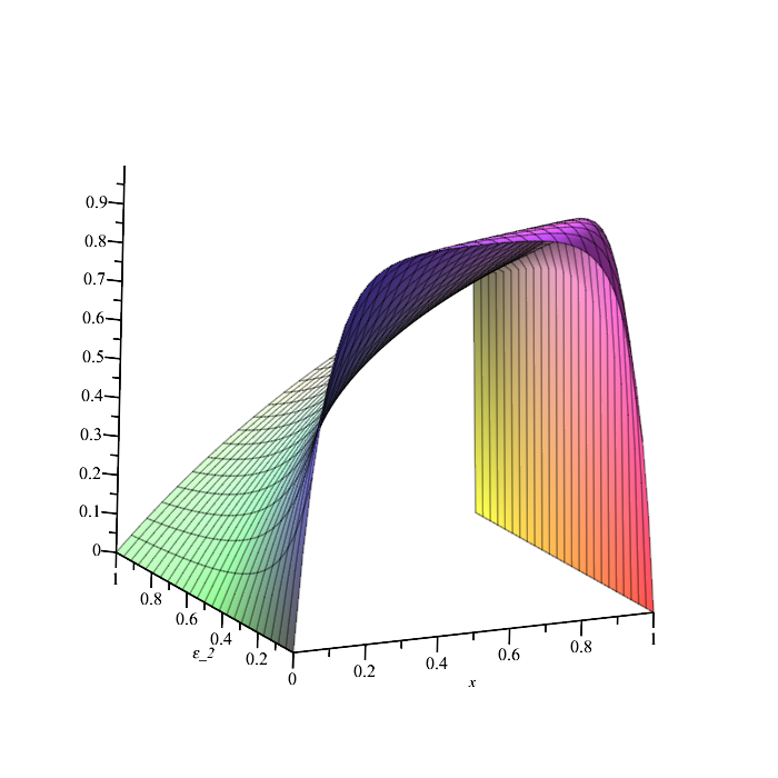
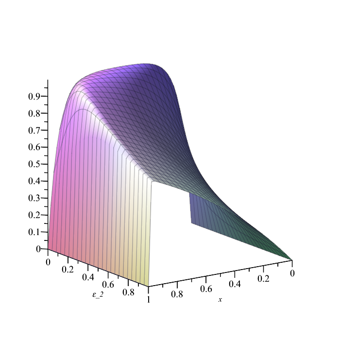
As a final question, we would like to see what happens when we fix ε1≪1\varepsilon_{1}\ll 1 and consider ε2∈(0,1]\varepsilon_{2}\in(0,1]. In Figure 1 we show the solution of the BVP

−0.005​u′′​(x)+ε2​u′​(x)+u⁡(x)\displaystyle-0.005u^{\prime\prime}(x)+\varepsilon_{2}u^{\prime}(x)+u(x) =\displaystyle= 1,x∈(0,1)\displaystyle 1,\>x\in(0,1)
u⁡(0)=u⁡(1)\displaystyle u(0)=u(1) =\displaystyle= 0,\displaystyle 0,

for ε2∈(0,1]\varepsilon_{2}\in(0,1].

Refer to caption

Refer to caption

Figure 1: The solution u⁡(x)u(x) as a function of xx and ε2\varepsilon_{2} (different viewing angles).

The figure shows that the trasition between regimes appears “seamless”, in the following sense: as ε2\varepsilon_{2} takes on values in (0,1](0,1], the solution uu “smoothly moves” from one regime to the other, based on the relationship between ε2\varepsilon_{2} and (the fixed, but small) ε1\varepsilon_{1}. In particular:

  • •

    If ε2=1\varepsilon_{2}=1, then we have a convection-diffusion problem, and we have a layer of width O⁡(ε1)O(\varepsilon_{1}) at the outflow boundary. (This is clearly visible in Figure 1, on the right.)

  • •

    If 1>ε2>ε11>\varepsilon_{2}>\sqrt{\varepsilon_{1}}, then we have a reaction-convection-diffusion problem, with layers of different width at each endpoint.

  • •

    If 0<ε2≤ε10<\varepsilon_{2}\leq\sqrt{\varepsilon_{1}}, then we have a reaction-diffusion problem, with layers of width O⁡(ε1)O(\sqrt{\varepsilon_{1}}) at each endpoint. (See Figure 1, on the left.)

The error bounds of the previous sections allow us to state the following:

Proposition 16.

Let ε1≪1\varepsilon_{1}\ll 1 be fixed, and let uu be the solution of (1)–(2) under the assumption (3). Then for any ε2∈(0,1)\varepsilon_{2}\in(0,1), there exist positive constants K1,K2,K3,δK_{1},K_{2},K_{3},\delta, independent of ε1,ε2\varepsilon_{1},\varepsilon_{2}, such that

u=uS+uB​L±+uR.u=u_{S}+u^{\pm}_{BL}+u_{R}.

The smooth part uSu_{S}, satisfies for any n∈ℕn\in\mathbb{N} , ε2∈(0,1)\varepsilon_{2}\in(0,1),

‖uS(n)‖∞,I≲K1n​n!.\left\|u_{S}^{(n)}\right\|_{\infty,I}\lesssim K_{1}^{n}n!.

The boundary layer parts uB​L±u^{\pm}_{BL}, satisfy for any n∈ℕn\in\mathbb{N} and

  • •

    ∀ε2∈(0,ε1],x∈I¯\forall\;\;\varepsilon_{2}\in(0,\sqrt{\varepsilon_{1}}],\;x\in\overline{I},

    |(uB​L±)(n)(x)|≲K2nn!ε1−n/2e−β dist (x,∂I)/ε1,\left|(u_{BL}^{\pm})^{(n)}(x)\right|\lesssim K_{2}^{n}n!\varepsilon_{1}^{-n/2}e^{-\beta\text{ dist }(x,\partial I)/\sqrt{\varepsilon_{1}}},
  • •

    ∀ε2∈(ε1,1),x∈I¯\forall\;\;\varepsilon_{2}\in(\sqrt{\varepsilon_{1}},1),\;x\in\overline{I},

    |(uB​L−)(n)(x)|≲K2nn!ε2−ne−βx/ε2,|(uB​L+)(n)|≲K2nn!(ε1ε2)−ne−β(1−x)ε2/ε1.\left|(u_{BL}^{-})^{(n)}(x)\right|\lesssim K_{2}^{n}n!\varepsilon_{2}^{-n}e^{-\beta x/\varepsilon_{2}}\;,\;\left|(u_{BL}^{+})^{(n)}\right|\lesssim K_{2}^{n}n!\left(\frac{\varepsilon_{1}}{\varepsilon_{2}}\right)^{-n}e^{-\beta(1-x)\varepsilon_{2}/\varepsilon_{1}}.

The remainder uRu_{R}, satisfies for any n∈ℕn\in\mathbb{N}, ε2∈(0,1)\varepsilon_{2}\in(0,1),

∥uR∥∞,∂I+∥uR∥0,I+min{ε2,ε1}∥uR′∥0,I≲max{e−δε2/ε1,e−δ/ε2}.\|u_{R}\|_{\infty,\partial I}+\|u_{R}\|_{0,I}+\min\{\varepsilon_{2},\sqrt{\varepsilon_{1}}\}\|u^{\prime}_{R}\|_{0,I}\lesssim\max\{e^{-\delta\varepsilon_{2}/\varepsilon_{1}},e^{-\delta/\varepsilon_{2}}\}.

4 Conclusions

We considered a two-point, singularly perturbed, reaction-convection-diffusion problem with analytic input data, and we derived regularity results for its solution. Based on the relationship between the singular perturbation parameters, the problem becomes convection-diffusion, reaction-diffusion or reaction-convection-diffusion, as shown in Table 1. We provided estimates for all three cases (regimes), which reveal the analytic nature of the solution and give derivative bounds which are explicit in the differentiation order as well as the singular perturbation parameters. Such estimates are necessary for the construction and analysis of high order numerical methods, such as h​php FEM (see, e.g. [16]).

References

  • [1] M. Brdar and H. Zarin, A singularly perturbed problem with two parameters on a Bakhvalov-type mesh, J. Comp. Appl. Math., 292 (2016) 307–319.
  • [2] J. L. Garcia, E. O’Riordan and M. L. Pickett, A parameter robust high order numerical method for a singularly perturbed two parameter problem, Appl. Num. Math., 56 (2006) 962–980.
  • [3] T. Linß, Layer-adapted meshes for reaction-convection-diffusion problems, Lecture Notes in Mathematics 1985, Springer-Verlag, 2010.
  • [4] T. Linß and H. G. Roos, Analysis of a finite difference scheme for a singularly perturbed problem with two small parameters, Comput. Meth. Appl. Math., 289 (2004) 355–366.
  • [5] J. M. Melenk, hp Finite Element Methods for Singular Perturbations, Lecture Notes in Mathematics 1796, Springer-Verlag, 2002.
  • [6] J. M. Melenk, On the robust exponential convergence of hp finite element methods for problems with boundary layers, IMA J. Num. Anal., 17 (1997) 577–601.
  • [7] J. M. Melenk and C. Schwab, An hp Finite Element Method for convection-diffusion problems in one-dimension, IMA J. Num. Anal., 19 (1999) 425–453.
  • [8] R. E. O’Malley, Singular Perturbation Methods for Ordinary Differential Equations, Springer-Verlag (1991).
  • [9] J. J. H. Miller, E. O’Riordan and G. I. Shishkin, Fitted Numerical Methods Singular Perturbation Problems, World Scientific, 1996.
  • [10] K. W. Morton, Numerical Solution of Convection-Diffusion Problems, Volume 12 of Applied Mathematics and Mathematical Computation, Chapman & Hall, 1996.
  • [11] F. W. J. Olver, Asymptotics and Special Functions, Academic Press, 1974.
  • [12] E. O’Riordan, M. L. Pickett and G. I. Shishkin, Singularly perturbed problems modelling reaction-convection-diffusion processes, Comput. Meth. Appl. Math., 3 (2003) 424–442.
  • [13] H.-G. Roos, M. Stynes, and L. Tobiska. Robust numerical methods for singularly perturbed differential equations, volume 24 of Springer Series in Computational Mathematics. Springer-Verlag, Berlin, second edition, 2008. Convection-diffusion-reaction and flow problems.
  • [14] H.-G. Roos and Z. Uzelac, The SDFEM for a Convection-Diffusion Problem with Two Small Parameters, Comput. Methods Appl. Math., 3 (2003) 443–458.
  • [15] I. Sykopetritou, An h​php finite element method for a second order singularly perturbed boundary value problem with two small parameters, Ph.D. Dissertation, Department of Mathematics & Statistics, University of Cyprus, expected (2024).
  • [16] I. Sykopetritou and C. Xenophontos, An hp finite element method for a convection-reaction-diffusion singularly perturbed problem with two small parameters, Int. J. Numer. Anal. Model., 18 (2021) 481–499.
  • [17] Lj. Teofanov and H.-G. Roos, An elliptic singularly perturbed problem with two parameters I: Solution decompostition, J. Comput. Appl. Math., 206 (2007) 1802–1097.
  • [18] Lj. Teofanov and H.-G. Roos, An elliptic singularly perturbed problem with two parameters II: Robust finite element solution, J. Comput. Appl. Math., 212 (2008) 374–389.