Cyclic Szekeres Universes

One proposal to solve the flatness and the horizon problems of our universe, that differs from the inflationary scenario guth, is the cyclic cosmological model cyc1. In the cyclic model, the universe undergoes an endless series of cycles of expansion and contraction, and the cosmic energy density and cosmic temperature remain finitely defined at any transition between expanding and contracting phases of the universe.

In the theory of general relativity cyclic universes can be constructed in the presence of a ghost field gyb. Ghost fields are exotic matter sources with negative energy density and also can have a parameter for the equation of state $w_{f}$ $=p/\rho$ for pressure $p$ and density $\rho,$ such that $w_{f}<-1$. There are various applications of ghost fields in classical and quantum cosmology s1; s2; s3; s4 and it is interesting to note that the stability of Einstein static universes changes in the presence of a ghost field. More specifically, in jts it was found that there exact solutions which describe an oscillation around an Einstein static solution for a closed Friedmann–Lemaître–Robertson–Walker universe (FLRW) when a radiation-ghost field ($w_{f}=1/3,\rho<0$) exists. More recently, the behaviour of cyclic mixmaster universes was studied in jkm; jkm2 in the presence of ghost fields.

In this work, we study the existence of ghost fields in inhomogeneous dust universes sz00 by assuming a “silent universe” silent1 with dust and a radiation-like ghost matter source. More specifically, we focus on the existence and stability of Szekeres-like cyclic universes. Szekeres universes szek0; szafron describe exact inhomogeneous solutions in general relativity which does not admit any isometry musta. These exact solutions are categorized in two large families of spacetimes, the inhomogeneous Kantowski-Sachs solutions and the inhomogeneous FLRW solutions. Various applications of the Szekeres universes can be found in sz2; sz2a; sz3; sz4; sz5; sz6; sz7. A detailed analysis of the conservation laws and the dynamics of the Szekeres system was performed recently in f1; f2. The results of f1 were applied in f3 to quantize the Szekeres system for the first time.

A generalization of the Szekeres solutions in the presence of a cosmological constant was presented in barcc; while the inclusion of a fluid source with heat flow in Szekeres universes was made in hf1. Recently, the case of the Szekeres inhomogeneous dust model with a homogeneous scalar field was studied in jdbsc. In jdbsc it was found that there exists only one family of solutions which describe inhomogeneous universes and they generalise the FLRW family. By contrast, the Szekeres family of solutions of Kantowski-Sachs type describe spatially homogeneous universes when the ghost field is added to the dust.

In the following, we consider the Szekeres system with a dust fluid and a homogeneous ghost matter source with constant parameter for the equation of state. We solve the gravitational field equations analytically and we find that the two families of solutions are those of homogeneous Kantowski-Sachs and inhomogeneous FLRW spacetimes. These results are similar to that of the Szekeres model with a homogeneous scalar field jdbsc. For the inhomogeneous FLRW-like solution we are able to write the solution in a closed form. More specifically, we find again that for a closed FLRW-like universe there exists a periodic solution around a static universe. Furthermore, from the stability analysis we find that all the solutions in which the expansion rate $\theta$ changes sign are unstable. We perform that analysis by studying the field equations in dimensionless variables different from those of the $H-$normalization silent1.

The plan of the paper is as follows. In Section II we define our cosmological model which is that of the Szekeres metric with a homogeneous and isotropic ghost field with constant parameter for the equation of state. The requirement of homogeneity for the ghost field provides a first constraint on the unknown functions in the line element for the geometry of the universe. In Section III we present the two families of spacetimes which describe the solutions of the field equations. The stability of the cyclic solutions is presented in Section IV. Finally, in Section V we discuss our results and we draw our conclusions.

In the context of general relativity we consider the action integral of the field equations to be

where $L_{m}$ is the Lagrangian density of a pressureless fluid term and $L_{G}$ describes an isotropic and homogeneous ghost ideal gas.

The Einstein field equations are

in which

where the Bianchi identity gives $\left(T^{\mu\nu\left(m\right)}+T^{\mu\nu\left(g\right)}\right)_{;\nu}=0$. Furthermore, by assuming that the two matter sources (dust and ghost field) are minimally coupled, we end up with two separate conservation equations:

For the background metric, we consider the following line element introduced by Szekeres szek0:

where functions of $A=A\left(t,r,y,z\right)$ and $B=B\left(t,r,y,z\right)$ are solutions of the Einstein’s field equations (2).

In terms of $1+3$ decomposition for the fluid sources we have

where $u^{\mu}=\delta_{t}^{\mu}$ is the comoving 4-velocity and $h_{\mu\nu}=g_{\mu\nu}+u_{\mu}u_{\nu}$ is the projective tensor, $\rho_{m}$ is the inhomogeneous dust density, and for the homogeneous ghost field we set $p_{g}\left(t\right)=\left(\gamma-1\right)\rho_{g}\left(t\right).$Both fluids share the same 4-velocity.

By substituting (6) into (4), we find

which implies jdbsc:

We proceed now with the presentation of the possible solutions for the Einstein field equations (2).

Szekeres spacetimes correspond to two families, the Kantowski-Sachs family with $\frac{\partial B}{\partial r}=0$ and the FLRW family in which $\frac{\partial B}{\partial r}\neq 0$. While in the Szekeres system the two spacetimes are inhomogeneous and do not admit any isometry, in jdbsc it was found that, if an isotropic scalar field is added to the dust source then the Kantowski-Sachs family of solutions must be spatially homogeneous, while an extra constraint on the functional form of the spacetime appears for the inhomogeneous FLRW family. In a similar way, the same two families of solutions are determined for the model considered here.

In particular, for the homogeneous Kantowski-Sachs family, the line element (5) simplifies to

with $c_{1},c_{2}$ constants, while the gravitational field equations reduce to those of the Kantowski-Sachs spacetime with two homogeneous perfect fluids ks011 whose solution gives the evolution of the scale factors¹¹ 1 Note that in the case of homogeneous perfect fluids, for the line element 10 the conservation equations (7)-(8) give $\rho_{m}(t)=\rho_{m0}a^{-1}b^{-2}$ and $\rho_{g}=\rho_{g0}a^{-\gamma}b^{-2\gamma}$, in which $\rho_{mo}$ and $\rho_{go}$ are constants of integration. $a(t)$ and $b(t)$. Moreover, the spatial curvature $K$ of the 2-dimensional line element $ds_{\left(2\right)}^{2}=\left(c_{1}\left(\left(y-y_{0}\right)^{2}+\left(z-z_{0}\right)^{2}\right)+c_{2}\right)^{-2}\left(dy^{2}+dz^{2}\right)$ is calculated to be²² 2 When $K=0$, the line element (10) describes the homogeneous Bianchi I spacetime, while, when $K>0$ , the line element (10) is that of the Bianchi III spacetime. $K=8c_{1}c_{2}$.

The nonlinearity of the field equations prevents us from finding closed-form solutions. However, for $K=0$ (or in the limit in which$~\frac{K}{b^{2}}\rightarrow 0$) under the transformation $a=u\left(\tau\right)v^{3}\left(\tau\right)$, $b=v^{3}\left(\tau\right),~dt=ab^{2}d\tau$ the gravitational field equations lead to

while $v\left(\tau\right)$ satisfies the two equations

and

where we have assumed $\gamma=\frac{4}{3}$for the ghost field. When we perform the coordinate transformation, $v\left(\tau\right)=e^{-\frac{u_{1}}{9}\tau}V\left(\tau\right)$, the second-order differential equation (13) is simplified to

which does not admit any periodic solutions. More specifically, it admits the unique critical point, for $\rho_{g0}<0$, $V_{c}=\left(\frac{2\left|\rho_{g0}\right|}{r_{0}}\right)^{\frac{1}{3}}$, which is a source point and describes an Einstein static universe. Now, in the case where $u_{1}=0$, we have $a\left(\tau\right)=v\left(\tau\right)$ so the Bianchi I spacetime reduces to the spatially flat homogeneous FLRW universe.

In Fig. 1 the qualitative time-evolution of the volume $V\left(t\right)$, the expansion rate $\theta\left(t\right),$ and the shear $\sigma\left(t\right)$ are presented following a numerical simulation of the field equations for $K=0$, and $\left|\rho_{g0}\right|>\rho_{m0}$.

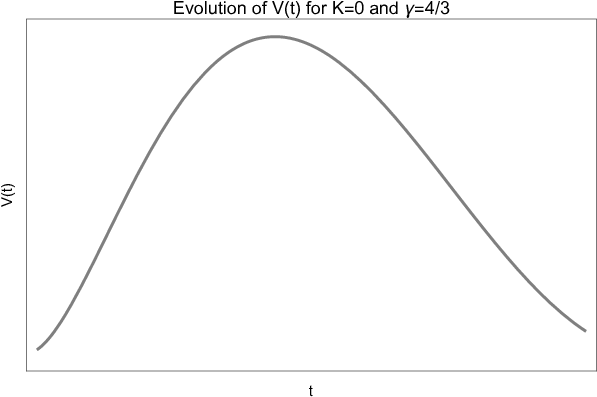
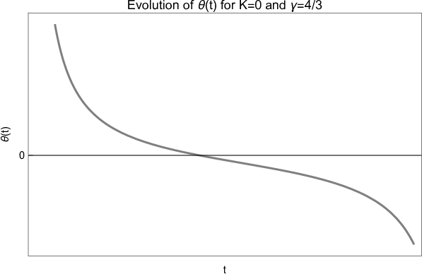
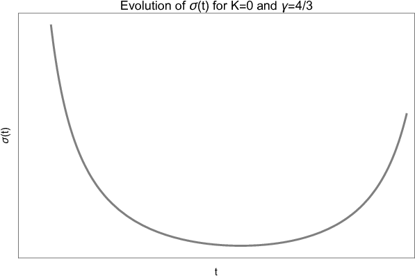
In the following section we find that solutions with volume expansion turning points, where $\theta\left(t_{0}\right)=0$ , exist for $K<0,$ but for different values of the barotropic parameter $\gamma$.

The second family of the Szekeres solutions is that of the inhomogeneous FLRW-like spacetimes, where the line element is given by the expression jdbsc

The spatial function $C\left(r,y,z\right)~$is given by the expression

where two of the four arbitrary functions, $\gamma_{1}\left(r\right)\rightarrow\gamma_{4}\left(r\right),$ are related to the spatial curvature, $K$, by

It is important to mention here that $K$ is a constant and not a function of $r$ as it is in the case of the Szekeres spacetimes. This difference arises because of the existence of the second (homogeneous ghost) fluid source. Moreover, the evolution of scale factor, $a\left(t\right),$ is described by Friedmann’s equations with two homogeneous perfect fluids; its general analytic solution is expressed in terms of elliptic integrals.

However, in the particular case for which $\rho_{g}$ describes a radiation ghost field, i.e., $\gamma=\frac{4}{3}$, the exact form of the scale factor is given by the following simple expression jts; jkm

or by

where $\tau$ is the conformal time defined by $dt=a\left(\tau\right)d\tau$. The scale factor in $K=0$ solution increases towards a power law, with a minimum as $\tau\rightarrow 0$ at $a\left(0\right)=$ $\frac{\left|\rho_{g0}\right|}{\rho_{m0}}$. For zero spatial curvature the scale factor has a minimum at $a_{\min}^{\left(k=0\right)}=\frac{\left|\rho_{g0}\right|}{\rho_{m0}}$. For positive spatial curvature, ($K=1$), the solution (18) is real when $\left(\rho_{m0}\right)^{2}>12\left|\rho_{g0}\right|$ and it is also a periodic solution with minimum and maximum of $a(\tau$) and $a(t)$ at

and the scale factor can be written as jts

so we can see that the scale factor oscillates around the static solution $a^{\left(k=1\right)}\left(0\right)=\left(a_{\max}^{\left(k=1\right)}+a_{\min}^{\left(k=1\right)}\right)$ with arbitrary amplitude. Hence these solutions show the stability of the Einstein static universe to these bounded oscillations but they only occur when a ghost field is present.

Note that the quantities $a_{\max}^{\left(k=1\right)}$ and $a_{\min}^{\left(k=1\right)}$ are not spatially varying because they depend on the constant quantities $\rho_{m0}$ and $\left|\rho_{g0}\right|$.

Finally, for $K=-1$, solution (18) is real if and only if $\rho_{m0}<12\left|\rho_{g0}\right|$ and the scale factor then simplifies to

which increases exponentially as $\tau\rightarrow\infty$.

We continue our analysis by studying the stability of these particular solutions with emphasis on the cyclic solutions.

We have seen that the addition of the ghost field to the Szekeres universes can create new cyclic solutions, or solutions in which the volume expansion rate, $\theta\left(t\right),$ can go to zero and change sign. In this section we perform a dynamical analysis of the kinematic quantities for the gravitational field equations. Here, the solutions with $\theta=0$ appear and we are able to study their stability.

In terms of the kinematic quantities $\theta,~\sigma,~\mathcal{E}$, $\rho_{m}$ and³³ 3 Here, $\sigma$ denotes the shear scalar and $\mathcal{E}$ is the scalar for the electric part of the Weyl tensor. $\rho_{g},$ the Szekeres field equations (2) are expressed as follows ellis1; ellis2

where ${}^{\left(3\right)}R$ denotes the curvature of the three-dimensional hypersurfaces.

We proceed by choosing the new dimensionless variables alg, $\omega_{m},\omega_{r}$ and $\omega_{R}$ defined via

and $\beta,\mathcal{E}$ and $h$ by

so the gravitational field equations become an autonomous system:

and there is a first integral

where the new time variable, $\zeta$, is defined as $dt=\left(\sqrt{1+\theta^{2}}\right)d\zeta.$

This normalization of the variables differs from the usual $H-$normalization ellis1; cope because now it is possible to determine critical points also in the surface where $\theta=0$, where $h=0$. Furthermore, parameters $\omega_{m}$, $\omega_{g}$ and $\omega_{R}$ are related to the familiar energy-density parameters $\Omega_{m},~\Omega_{g}$ and $\Omega_{R}$ as follows:

We are interested in the critical points for the system (31)-(35) when $\theta$ is zero. They can be easily computed:

and

These points $P_{1}~$and $P_{2}$ describe Einstein static universes.

However, in addition to those two critical points there is a family of critical points where $h^{2}=1$. These correspond to the Szekeres universes when $\omega_{g}=0$ and to the Szekeres-Szafron universes szafron when $\omega_{m}=0$. Moreover, we find that there is no critical point where $\omega_{m}\omega_{g}\neq 0$.

Now we discuss the stability and the physical parameters of the points $P_{1}$ and $P_{2}$.

a. At point $P_{1}~$the anisotropic parameter $\beta~$ is not a constraint, which means that $P_{1}$ describes a surface of critical points on the phase-space. Since $\beta$ is unconstrained, point $P_{1}$ can describe solutions in the Kantowski-Sachs family and in the FLRW-like family. From the algebraic equation (36), we can derive the parameter $\omega_{R}$, namely,

Hence, the final geometry of the solution at $P_{1}~$depends upon the equation of state parameter,$\gamma$, for the ghost field, $\rho_{g}$. If we assume that $\beta\neq 0$, then for $\gamma=\frac{4}{3}$ the solution at point $P_{1}$ describes a Bianchi I spacetime, for $\gamma>\frac{4}{3}$, the geometry is that of Bianchi III, while, when $\gamma<\frac{4}{3},$ it follows that $\omega_{R}<0$, which means that the ${}^{\left(3\right)}R<0$ and the solution at point $P_{1}$ describes a Kantowski-Sachs universe. Furthermore, at the special limit where $\beta=0$, $P_{1}$ describes the Minkowski spacetime. We study the stability of the solution at $P_{1}$ in the four-dimensional subspace $\left\{\beta,\varepsilon,\omega_{m},\omega_{g}\right\}$ when $h\rightarrow 0$. We find that there exists an eigenvalue, positive real-valued, for the matrix which defines the linearized system. Therefore, the solution at $P_{1}$ is unstable in the 4-dimensional subspace $\left\{\beta,\varepsilon,\omega_{m},\omega_{g}\right\}$ and consequently also in the 5-dimensional space in which the dynamical system evolves. Two-dimensional phase-space diagrams are presented in Figures 2-5, from which it is clear that $P_{1}$ describes an unstable Einstein static solution. Moreover, from the phase-space diagrams we observe that unstable oscillatory behaviours exist around $P_{1}.$ The figures are for $\gamma=\frac{4}{3}$, Figs. 2 and 3 are in the surface $\omega_{m}-h$, $\omega_{g}-h$, respectively, Fig. 4 is in the surface $\beta-\varepsilon$ and vectors in Fig. 5 are on the surface $\beta-h$.

b. The solution at point $P_{2}$ describes an isotropic static universe because $\beta=\varepsilon=0$, and more specifically it is the inhomogeneous FLRW space with positive spatial curvature, i.e., $\omega_{R}=-\omega_{g}$. We remark that $P_{2}$, like point $P_{1}$, is actually a surface – a family of solutions where $\omega_{m}=-2\omega_{g}$ but with $\omega_{R}=\frac{\omega_{m}}{2}$, which means that the spatial 3-curvature is positive. In order to study the stability of the solution we calculate the eigenvalues of the linearized system and they are

Hence, there exists always a positive eigenvalue and so we can infer that the solution at $P_{2}$ is unstable. However, one of the eigenvalues has nonzero imaginary part (because $\omega_{m}=-2\omega_{g}$) which means that periodic behaviour exists. In particular the imaginary eigenvalues are in the $\omega_{g}-h$ surface, and indeed periodic behaviour is observed in Fig. 6. This means that small perturbations around $P_{2}$ in the $\omega_{g}-h$ surface give a behaviour similar to that of the solution (21). In Figures 7 and 8 the phase-space diagrams in the $\omega_{m}-h$ and $\beta-h$ surfaces are presented, respectively.

We have considered the Szekeres dust universe with an additional homogeneous and isotropic ghost field. The equation of state parameter for the ghost field was assumed to be $p_{g}=\left(\gamma-1\right)\rho_{g}$ and $\rho_{g}<0$. We were able to simplify the gravitational field equations and determine the existence of two possible families of solutions. Unlike in the absence of the ghost field, the first family of solutions describes spatially homogeneous Kantowski-Sachs universes, while the second family of solutions describes inhomogeneous FLRW-like universes. The specific forms of the spacetimes are similar to those determined in the case of an homogeneous scalar field and dust in the Szekeres metricsjdbsc. However, the existence of the ghost field produces new possible behaviours for the scale factors of these universes. Specifically, it is possible to have Einstein-static solutions in the Kantowski-Sachs family while a cyclic solution was found analytically for the FLRW-like family of spacetimes.

By studying the critical points of the gravitational field equations expressed in terms of the kinematic quantities we have found two points which describe Einstein static solutions, points $P_{1}$ and $P_{2}$, which are sources. More specifically, $P_{1}$ and $P_{2}$ actually describe surfaces in the dynamical phase-space: $P_{1}$ exists for both of the families while $P_{2}$ describes an Einstein static solution in the FLRW family of solutions. While the Einstein solutions are unstable, from the numerical simulations it is easy to observe that for specific initial conditions around the critical points cyclic behaviour appears which is agreement with the cyclic solution determined analytically. These are the first studies, via exact solutions, of inhomogeneous oscillating universes. We have not introduced dissipative processes but entropy production could be introduced in order to study the evolution of cycle size and length as the universe evolves through successive maxima tol; BD; jkm; jkm2