跳到论文正文
W Papers独立论文阅读器 arXiv:1901.09109 论文正文 计算阅读时间 · 0%
引用这篇论文根据当前论文元数据生成,正式投稿前建议核对。


License: arXiv.org perpetual non-exclusive license
arXiv:1901.09109v6 [cs.LG] 28 May 2019

DADAM: A Consensus-based Distributed
Adaptive Gradient Method for Online Optimization

Parvin Nazari Thanks: Department of Mathematics & Computer Science, Amirkabir University of Technology, Email: p$_$nazari@aut.ac.ir    Davoud Ataee Tarzanagh Thanks:  Department of Mathematics & UF Informatics Institute, University of Florida, Email: tarzanagh@ufl.edu    George Michailidis Thanks:  Department of Statistics & UF Informatics Institute, University of Florida, Email: gmichail@ufl.edu

Adaptive gradient-based optimization methods such as Adagrad, Rmsprop, and Adam are widely used in solving large-scale machine learning problems including deep learning. A number of schemes have been proposed in the literature aiming at parallelizing them, based on communications of peripheral nodes with a central node, but incur high communications cost. To address this issue, we develop a novel consensus-based distributed adaptive moment estimation method (Dadam) for online optimization over a decentralized network that enables data parallelization, as well as decentralized computation. The method is particularly useful, since it can accommodate settings where access to local data is allowed. Further, as established theoretically in this work, it can outperform centralized adaptive algorithms, for certain classes of loss functions used in applications. We analyze the convergence properties of the proposed algorithm and provide a dynamic regret bound on the convergence rate of adaptive moment estimation methods in both stochastic and deterministic settings. Empirical results demonstrate that Dadam works also well in practice and compares favorably to competing online optimization methods.

Adaptive gradient method. Online learning. Distributed optimization. Regret minimization.

1 Introduction

Online optimization is a fundamental procedure for solving a wide range of machine learning problems [1, 2]. It can be formulated as a repeated game between a learner (algorithm) and an adversary. The learner receives a streaming data sequence, sequentially selects actions, and the adversary reveals the convex or nonconvex losses to the learner. A standard performance metric for an online algorithm is regret, which measures the performance of the algorithm versus a static benchmark [3, 2]. For example, the benchmark could be an optimal point of the online average of the loss (local cost) function, had the learner known all the losses in advance. In a broad sense, if the benchmark is a fixed sequence, the regret is called static. Recent work on online optimization has investigated the notion of dynamic regret [3, 4, 5]. Dynamic regret can take the form of the cumulative difference between the instantaneous loss and the minimum loss. For convex functions, previous studies have shown that the dynamic regret of online gradient-based methods can be upper bounded by O⁡(T​DT)O(\sqrt{TD_{T}}), where DTD_{T} is a measure of regularity of the comparator sequence or the function sequence [3, 4, 6]. This bound can be improved to O⁡(DT)O(D_{T}) [7, 8], when the cost function is strongly convex and smooth.

Decentralized nonlinear programming has received a lot of interest in diverse scientific and engineering fields [9, 10, 11, 12]. The key problem involves optimizing a cost function f⁡(x)=1n​∑i=1nfi​(x)f(x)=\frac{1}{n}\sum_{i=1}^{n}f_{i}(x), where x∈ℝpx\in{\mathbb{R}}^{p} and each fif_{i} is only known to the individual agent ii in a connected network of nn agents. The agents collaborate by successively sharing information with other agents located in their neighborhood with the goal of jointly converging to the network-wide optimal argument [13]. Compared to optimization procedures involving a fusion center that collects data and performs the computation, decentralized nonlinear programming enjoys the advantage of scalability to the size of the network used, robustness to the network topology, and privacy preservation in data-sensitive applications.

A popular algorithm in decentralized optimization is gradient descent which has been studied in [13, 14]. Convergence results for convex problems with bounded gradients are given in [15], while analogous convergence results even for nonconvex problems are given in [16]. Convergence can be accelerated by using corrected update rules and momentum techniques [17, 18, 19, 20]. The primal-dual [21, 22], Admm [23, 24] and zero-order [25] approaches are related to the dual decentralized gradient method [14]. We also point out recent work on a very efficient consensus-based decentralized stochastic gradient (Dsgd) method for deep learning over fixed topology networks [20] and earlier work on decentralized gradient methods for nonconvex deep learning problems [26]. Further, under some mild assumptions, [26] shows that decentralized algorithms can be faster than their centralized counterparts for certain stochastic nonconvex loss functions.

Appropriately choosing the learning rate that scales coordinates of the gradient and the way of updating them are critical issues that impact the performance of first [27, 28, 29] and second order optimization procedures [30, 31, 32]. Indeed, an adaptive learning rate is advantageous, which led to the development of a family of widely-used methods including Adagrad [27], Adadelta [33], Rmsprop [29], Adam [28] and Amsgrad [34]. Numerical results show that Adam can achieve significantly better performance compared to Adagrad, Adadelta, and Rmsprop for minimizing non-stationary objectives and problems with very noisy and/or sparse gradients. However, it has been recently demonstrated that Adam can fail to converge even in simple convex settings [35, 34]. To tackle this issue, some sufficient conditions such as decreasing the learning rate [34, 36, 37, 38, 39] or adopting a big batch size [40, 41] have been proposed to provide convergence guarantees for Adam and its variants.

In this paper, we develop and analyze a new consensus-based distributed adaptive moment estimation (Dadam) method that incorporates decentralized optimization and leverages a variant of adaptive moment estimation methods [27, 28, 42]. Existing distributed stochastic and adaptive gradient methods for deep learning are mostly designed for a central network topology [43, 44]. The main bottleneck of such a topology lies on the communication overload on the central node, since all nodes need to concurrently communicate with it. Hence, performance can be significantly degraded when network bandwidth is limited. These considerations motivate us to study an adaptive algorithm for network topologies, where all nodes can only communicate with their neighbors and none of the nodes is designated as “central”. Therefore, the proposed method is suitable for large scale machine learning problems, since it enables both data parallelization and decentralized computation.

Next, we briefly summarize the main technical contributions of the work.

  • -

    The first main result (Theorem 5) provides guarantees of Dadam for constrained convex minimization problems defined over a closed convex set 𝒳\mathcal{X}. We provide the convergence bound in terms of dynamic regret and show that when the data features are sparse and have bounded gradients, our algorithm’s regret bound can be considerably better than the ones provided by standard mirror descent and gradient descent methods [13, 4, 5]. It is worth mentioning that the regret bounds provided for adaptive gradient methods [27] are static and our results generalize them to dynamic settings.

  • -

    Theorem 8 provides a novel local regret analysis for distributed online gradient-based algorithms for constrained nonconvex minimization problems computed over a network of agents. Specifically, we prove that under certain regularity conditions, Dadam can achieve a local regret bound of order O~​(1T)\tilde{O}(\frac{1}{T}) for nonconvex distributed optimization. To the best of our knowledge, rigorous extensions of existing adaptive gradient methods to the distributed nonconvex setting considered in this work do not seem to be available.

  • -

    In this paper, we also present regret analysis for distributed optimization problems computed over a network of agents. Theorems 6 and 10 provide regret bounds of Dadam for problem (2) with stochastic gradients and indicate that the result of Theorems 5 and 8 hold true in expectation. Further, in Corollary 11 we show that Dadam can achieve a local regret bound of order O⁡(ξ2n​T+1T)O(\frac{\xi^{2}}{\sqrt{nT}}+\frac{1}{T}) for nonconvex stochastic optimization where ξ\xi is an upper bound on the variance of the stochastic gradients. Hence, Dadam outperforms centralized adaptive algorithms such as Adam for certain realistic classes of loss functions when TT is sufficiently large.

Note that the technical results established exhibit differences from those in [13, 14, 15, 16] with the notion of adaptive constrained optimization in online and dynamic settings.

The remainder of the paper is organized as follows. Section 2 gives a detailed description of Dadam, while Section 3 establishes its theoretical results. Section 4 explains a network correction technique for our proposed algorithm. Section 5 illustrates the proposed framework on a number of synthetic and real data sets. Finally, Section 6 concludes the paper.

The detailed proofs of the main results established are delegated to the Supplementary Material.

1.1 Mathematical Preliminaries and Notations.

Throughout the paper, ℝp\mathbb{R}^{p} denotes the pp-dimensional real space. For any pair of vectors x,y∈ℝp,⟨x,y⟩x,y\in\mathbb{R}^{p},\,\,\langle x,y\rangle indicates the standard Euclidean inner product. We denote the ℓ1\ell_{1} norm by ‖X‖1=∑i​j|xi​j|\|X\|_{1}=\sum_{ij}|x_{ij}|, the infinity norm by ‖X‖∞=maxi​j⁡|xi​j|\|X\|_{\infty}=\max_{ij}|x_{ij}|, and the Euclidean norm by ‖X‖=∑i​j|xi​j|2\|X\|=\sqrt{\sum_{ij}|x_{ij}|^{2}}. The above norms reduce to the vector norms if XX is a vector. The diameter of the set 𝒳\mathcal{X} is given by

γ∞=supx,y∈𝒳‖x−y‖∞.\gamma_{\infty}=\sup_{x,y\in\mathcal{X}}\|x-y\|_{\infty}. (1)

Let 𝒮+p\mathcal{S}_{+}^{p} be the set of all positive definite p×pp\times p matrices. Π𝒳,A​[x]\Pi_{\mathcal{X},A}~[x] denotes the Euclidean projection of a vector xx onto 𝒳\mathcal{X} for A∈𝒮+pA\in\mathcal{S}_{+}^{p}:

Π𝒳,A​[x]=arg​miny∈𝒳⁡‖A12​(x−y)‖.\Pi_{\mathcal{X},A}~\big[x\big]=\argmin_{y\in\mathcal{X}}\|A^{\frac{1}{2}}(x-y)\|.

The subscript tt is often used to denote the time step while yi,t,dy_{i,t,d} stands for the dd-th element of yi,ty_{i,t}. Further, yi,1:t,d∈ℝty_{i,1:t,d}\in\mathbb{R}^{t} is given by

yi,1:t,d=[yi,1,d,yi,2,d,…,yi,t,d]⊤.y_{i,1:t,d}=[y_{i,1,d},y_{i,2,d},\ldots,y_{i,t,d}]^{\top}.

We let gi,tg_{i,t} denote the gradient of ff at xi,tx_{i,t}. The ii-th largest singular value of matrix XX is denoted by σi​(X)\sigma_{i}(X). We denote the element in the ii-th row and jj-th column of matrix XX by [X]i​j[X]_{ij}. In several theorems, we consider a connected undirected graph 𝒢=(𝒱,ℰ)\mathcal{G}=(\mathcal{V},\mathcal{E}) with nodes 𝒱={1,2,…,n}\mathcal{V}=\{1,2,\ldots,n\} and edges ℰ\mathcal{E}. The matrix W∈ℝn×nW\in\mathbb{R}^{n\times n} is often used to denote the weighted adjacency matrix of graph 𝒢\mathcal{G}. The Hadamard (entrywise) and Kronecker product are denoted by ⊙\odot and ⊗\otimes, respectively. Finally, the expectation operator is denoted by 𝔼\mathbb{E}.

2 Problem Formulation and Algorithm

We develop a new online adaptive optimization method (Dadam) that employs data parallelization and decentralized computation over a network of agents. Given a connected undirected graph 𝒢=(𝒱,ℰ)\mathcal{G}=(\mathcal{V},\mathcal{E}), we let each node i∈𝒱i\in\mathcal{V} at time t∈[T]≡{1,…,T}t\in[T]\equiv\{1,\ldots,T\} holds its own measurement and training data bib_{i}, and set fi,t​(x)=1bi​∑j=1bifi,tj​(x)f_{i,t}(x)=\frac{1}{b_{i}}\sum_{j=1}^{b_{i}}f_{i,t}^{j}(x). We also let each agent ii holds a local copy of the global variable xx at time t∈[T]t\in[T], which is denoted by xi,t∈ℝpx_{i,t}\in\mathbb{R}^{p}. With this setup, we present a distributed adaptive gradient method for solving the minimization problem

minimizex∈𝒳F⁡(x)=1n​∑t=1T∑i=1nfi,t​(x),\minimize_{x\in\mathcal{X}}\quad F(x)=\frac{1}{n}\sum_{t=1}^{T}\sum_{i=1}^{n}f_{i,t}(x), (2)

where fi,t:𝒳→ℝf_{i,t}:\mathcal{X}\rightarrow\mathbb{R} is a continuously differentiable mapping on the convex set 𝒳\mathcal{X}.

Dadam uses a new distributed adaptive gradient method in which a group of nn agents aim to solve a sequential version of problem (2). Here, we assume that each component function fi,t:𝒳→ℝf_{i,t}:\mathcal{X}\rightarrow\mathbb{R} becomes only available to agent i∈𝒱i\in\mathcal{V}, after having made its decision at time t∈[T]t\in[T]. In the tt-th step, the ii-th agent chooses a point xi,tx_{i,t} corresponding to what it considers as a good selection for the network as a whole. After committing to this choice, the agent has access to a cost function fi,t:𝒳→ℝf_{i,t}:\mathcal{X}\rightarrow\mathbb{R} and the network cost is then given by ft​(x)=1n​∑i=1nfi,t​(x)f_{t}(x)=\frac{1}{n}\sum_{i=1}^{n}f_{i,t}(x). Note that this function is not known to any of the agents and is not available at any single location.

The procedure of our proposed method is outlined in Algorithm 1.

input :   x1∈𝒳x_{1}\in\mathcal{X}, step-sizes {αt}t=1T\{\alpha_{t}\}_{t=1}^{T}, decay parameters β1,β2,β3∈[0,1)\beta_{1},\beta_{2},\beta_{3}\in[0,1) and a mixing matrix WW satisfying (6);
for all i∈𝒱i\in\mathcal{V}, initialize moment vectors mi,0=υi,0=υ^i,0=0m_{i,0}=\upsilon_{i,0}=\widehat{\upsilon}_{i,0}=0 and xi,1=x1x_{i,1}=x_{1}; 1
for t←1t\leftarrow 1 to TT do 2
for i∈𝒱i\in\mathcal{V} do 3
    gi,t=∇fi,t​(xi,t)g_{i,t}=\nabla f_{i,t}(x_{i,t}); 4
      mi,t=β1​mi,t−1+(1−β1)​gi,tm_{i,t}=\beta_{1}m_{i,t-1}+(1-\beta_{1})g_{i,t}; 5
       υi,t=β2​υi,t−1+(1−β2)​gi,t⊙gi,t\upsilon_{i,t}=\beta_{2}\upsilon_{i,t-1}+(1-\beta_{2})g_{i,t}\odot g_{i,t}; 6
       υ^i,t=β3​υ^i,t−1+(1−β3)​max⁡(υ^i,t−1,υi,t)\widehat{\upsilon}_{i,t}=\beta_{3}\widehat{\upsilon}_{i,t-1}+(1-\beta_{3})\max(\widehat{\upsilon}_{i,t-1},\upsilon_{i,t}); 7
       xi,t+12=∑j=1n[W]i​j​xj,tx_{i,t+\frac{1}{2}}=\sum_{j=1}^{n}[W]_{ij}x_{j,t}; 8
       xi,t+1=Π𝒳,diag​(υ^i,t)​[xi,t+12−αt​mi,tυ^i,t]x_{i,t+1}=\Pi_{\mathcal{X},\sqrt{{\text{diag}(\widehat{\upsilon}_{i,t})}}}~\big[x_{i,t+\frac{1}{2}}-\alpha_{t}\frac{m_{i,t}}{\sqrt{\widehat{\upsilon}_{i,t}}}\big]; 9
       output : resulting parameter x¯=1n​∑i=1nxi,T+1\bar{x}=\frac{1}{n}\sum_{i=1}^{n}x_{i,T+1}
Algorithm 1 A new distributed adaptive moment estimation method (Dadam).

It is worth mentioning that Dadam includes decentralized variants of many well-known algorithms as special cases, including Adagrad, Rmsprop, Amsgrad, Sgd and Sgd with momentum. We also note that Dadam computes adaptive learning rates from estimates of both first and second moments of the gradients similar to Amsgrad. However, Dadam uses a larger learning rate in comparison to Amsgrad and yet incorporates the intuition of slowly decaying the effect of previous gradients on the learning rate. In particular, we design the update expression of the second moment estimate of the gradient to be

υ^i,t=β3​υ^i,t−1+(1−β3)​max⁡(υ^i,t−1,υi,t),\widehat{\upsilon}_{i,t}=\beta_{3}\widehat{\upsilon}_{i,t-1}+(1-\beta_{3})\max(\widehat{\upsilon}_{i,t-1},\upsilon_{i,t}), (3)

where β3∈[0,1)\beta_{3}\in[0,1). The decay parameter β3\beta_{3} is an important component of the Dadam framework, since it enables us to develop a convergent adaptive method similar to Amsgrad (β3=0\beta_{3}=0), while maintaining the efficiency of Adam (β3=1\beta_{3}=1).

Next, we introduce the measure of regret for assessing the performance of Dadam against a sequence of successive minimizers. In the framework of online convex optimization, the performance of algorithms is assessed by regret that measures how competitive the algorithm is with respect to the best fixed solution [45, 2]. However, the notion of regret fails to illustrate the performance of online algorithms in a dynamic setting. To overcome this issue, we consider a more stringent metric, the dynamic regret [4, 5, 3], in which the cumulative loss of the learner is compared against the minimizer sequence {xt∗}t=1T\{x^{*}_{t}\}_{t=1}^{T}, i.e.,

𝐑𝐞𝐠TC:=1n​∑i=1n∑t=1Tfi,t​(xi,t)−∑t=1Tft​(xt∗),{\bf Reg}^{C}_{T}:=\frac{1}{n}\sum_{i=1}^{n}\sum_{t=1}^{T}f_{i,t}(x_{i,t})-\sum_{t=1}^{T}f_{t}(x^{*}_{t}),

where xt∗=arg​minx∈𝒳⁡ft​(x)x^{*}_{t}=\argmin_{x\in\mathcal{X}}f_{t}(x).

On the other hand, in the framework of nonconvex optimization, it is common to state convergence guarantees of an algorithm towards a ζ\zeta-approximate stationary point; that is, there exists some iterate xi,tx_{i,t} for which ‖∇ft​(xi,t)‖≤ζ\|\nabla f_{t}(x_{i,t})\|\leq\zeta. Influenced by [46], we provide the definition of projected gradient and introduce local regret next, a new notion of regret which quantifies the moving average of gradients over a network.

Definition 1.

(Local Regret). Assume fi:𝒳→ℝf_{i}:\mathcal{X}\rightarrow\mathbb{R} is a differentiable function on a closed convex set 𝒳⊆ℝp\mathcal{X}\subseteq\mathbb{R}^{p}. Given a step-size α>0\alpha>0, we define G𝒳​(x,fi,α):𝒳→ℝpG_{\mathcal{X}}(x,f_{i},\alpha):\mathcal{X}\rightarrow\mathbb{R}^{p} the projected gradient of fif_{i} at xx, by

G𝒳​(x,fi,α)=υ^iα​(x−xi+),∀i∈𝒱,G_{\mathcal{X}}(x,f_{i},\alpha)=\frac{\sqrt{\widehat{\upsilon}_{i}}}{\alpha}(x-x_{i}^{+}),\qquad\forall i\in\mathcal{V}, (4)

with

xi+=argminy∈𝒳​{⟨y,miυ^i⟩+12​α​‖y−∑j=1n[W]i​j​xj‖2},x_{i}^{+}=\textnormal{argmin}_{y\in\mathcal{X}}\{\langle y,\frac{m_{i}}{\sqrt{\widehat{\upsilon}_{i}}}\rangle+\frac{1}{2\alpha}\|y-\sum_{j=1}^{n}[W]_{ij}x_{j}\|^{2}\}, (5)

where mim_{i} and υ^i\widehat{\upsilon}_{i} are defined in Algorithm 1. Then, the local regret of an online algorithm is given by

𝐑𝐞𝐠TN:=1n​∑i=1nmint∈[T]⁡‖G𝒳​(xi,t,f¯i,t,αt)‖2,{\bf Reg}^{N}_{T}:=\frac{1}{n}\sum_{i=1}^{n}\min_{t\in[T]}\|G_{\mathcal{X}}(x_{i,t},\bar{f}_{i,t},\alpha_{t})\|^{2},

where f¯i,t​(xi,t)=1t​∑s=1tfi,s​(xi,t)\bar{f}_{i,t}(x_{i,t})=\frac{1}{t}\sum_{s=1}^{t}f_{i,s}(x_{i,t}) is an aggregate loss.

We analyze the convergence of Dadam as applied to minimization problem (2) using regrets 𝐑𝐞𝐠TC{\bf Reg}^{C}_{T} and 𝐑𝐞𝐠TN{\bf Reg}^{N}_{T}. Note that Dadam is initialized at xi,1=0x_{i,1}=0 to keep the presentation of the convergence analysis clear. In general, any initialization can be selected for implementation purposes.

3 Convergence Analysis

Next, we establish convergence properties of Dadam under the following assumptions:

Assumption 2.

The weighted adjacency matrix WW of graph 𝒢=(𝒱,ℰ)\vphantom{\sum^{N}}\mathcal{G}=(\mathcal{V},\mathcal{E}) is doubly stochastic with a positive diagonal. Specifically, the information received from agent j≠ij\not=i, [W]i​j\vphantom{\sum^{N}}[W]_{ij} satisfies

∑i=1n[W]i​j=∑j=1n[W]i​j=1,[W]j​j>0.\sum_{i=1}^{n}[W]_{ij}=\sum_{j=1}^{n}[W]_{ij}=1,\qquad[W]_{jj}>0. (6)
Assumption 3.

For all i∈𝒱i\in\mathcal{V} and t∈[T]t\in[T], the function fi,t​(x)f_{i,t}(x) is differentiable over 𝒳\mathcal{X}, and has Lipschitz continuous gradient on this set, i.e., there exists ρ<∞\rho<\infty so that

‖∇fi,t​(x)−∇fi,t​(y)‖≤ρ​‖x−y‖,∀x,y∈𝒳.\|\nabla f_{i,t}(x)-\nabla f_{i,t}(y)\|\leq\rho\|x-y\|,\qquad\forall x,y\in\mathcal{X}.

Further, there exists L<∞L<\infty such that

|fi,t​(x)−fi,t​(y)|≤L​‖x−y‖,∀x,y∈𝒳.|f_{i,t}(x)-f_{i,t}(y)|\leq L\|x-y\|,\qquad\forall x,y\in\mathcal{X}. (7)
Assumption 4.

For all i∈𝒱i\in\mathcal{V} and t∈[T]t\in[T], the stochastic gradient denoted by 𝐠=∇fi,t​(xi,t){\bm{g}}={\bm{\nabla}}f_{i,t}(x_{i,t}), satisfies

   𝔼⁡[∇fi,t​(xi,t)|ℱt−1]=∇fi,t​(xi,t),\displaystyle\mathbb{E}\left[\vphantom{\left\lVert{\bm{\nabla}}f_{i,t}(x_{i,t})\right\rVert_{*}^{2}}{\bm{\nabla}}f_{i,t}(x_{i,t})\big|\mathcal{F}_{t-1}\right]=\nabla f_{i,t}(x_{i,t}),
𝔼⁡[‖∇fi,t​(xi,t)‖2|ℱt−1]≤ξ2,\displaystyle\mathbb{E}\left[\left\lVert{\bm{\nabla}}f_{i,t}(x_{i,t})\right\rVert^{2}\big|\mathcal{F}_{t-1}\right]\leq\xi^{2},

where ℱt\mathcal{F}_{t} is the ξ\xi-field containing all information prior to the onset of round t+1t+1.

3.1 Convex Case

Next, we focus on the case where for all i∈𝒱i\in\mathcal{V} and t∈{1,…,T}t\in\{1,\ldots,T\}, the agent ii at time tt has access to the exact gradient gi,t=∇fi,t​(xi,t)g_{i,t}=\nabla f_{i,t}(x_{i,t}).

Theorems 5 and 6 characterize the hardness of the problem via a complexly measure that captures the pattern of the minimizer sequence {xt∗}t=1T\{x^{*}_{t}\}_{t=1}^{T}, where xt∗=arg​minx∈𝒳⁡ft​(x)x^{*}_{t}=\argmin_{x\in\mathcal{X}}f_{t}(x). Subsequently, we would like to provide a regret bound in terms of

DT,d=∑t=1T−1|xt+1,d∗−xt,d∗|ford∈{1,…,p},D_{T,d}=\sum_{t=1}^{T-1}|x^{*}_{t+1,d}-x^{*}_{t,d}|\qquad\text{for}\qquad d\in\{1,...,p\}, (8)

which represents the variations in {xt∗}t=1T\{x^{*}_{t}\}_{t=1}^{T}.

Further, the following theorems establish a tight connection between the convergence rate of distributed adaptive methods and the spectral properties of the underlying network. The inverse dependence on the spectral gap 1−σ2​(W)1-\sigma_{2}(W) is quite natural and for many families of undirected graph, we can give order-accurate estimate on 1−σ2​(W)1-\sigma_{2}(W) [[47], Proposition 5], which translate into estimates of convergence time.

Theorem 5.

Suppose Assumption 2 holds and the parameters β1,β2∈[0,1)\beta_{1},\beta_{2}\in[0,1) satisfy η=β1β2<1\eta=\frac{\beta_{1}}{\sqrt{\beta_{2}}}<1. Let β1,t=β1​λt−1,λ∈(0,1)\beta_{1,t}=\beta_{1}\lambda^{t-1},\lambda\in(0,1) and ‖∇fi,t​(xt)‖∞≤G∞\|\nabla f_{i,t}(x_{t})\|_{\infty}\leq G_{\infty} for all i∈𝒱i\in\mathcal{V} and t∈{1,…,T}t\in\{1,\ldots,T\}. Then, using a step-size αt=αt\alpha_{t}=\frac{\alpha}{\sqrt{t}} for the sequence xi,tx_{i,t} generated by Algorithm 1, we have

𝐑𝐞𝐠TC\displaystyle{\bf Reg}^{C}_{T} ≤α​1+log⁡T2​n​(1−β2)​(1−β3)∑d=1p∥g1:T,d∥\displaystyle\leq\frac{\alpha\sqrt{1+\log T}}{2\sqrt{n}\sqrt{(1-\beta_{2})(1-\beta_{3})}}\sum_{d=1}^{p}\|g_{1:T,d}\|
+∑d=1pG∞​γ∞​(1+γ∞/(2​α))(1−β1)2​(1−λ)2+∑d=1pγ∞​(γ∞+DT,d)n​(1−β1)​αT​υ^T,d\displaystyle+\sum_{d=1}^{p}\frac{G_{\infty}\gamma_{\infty}(1+{\gamma_{\infty}}/{(2\alpha)})}{(1-\beta_{1})^{2}(1-\lambda)^{2}}+\sum_{d=1}^{p}\frac{\gamma_{\infty}(\gamma_{\infty}+D_{T,d})}{\sqrt{n}(1-\beta_{1})\alpha}\sqrt{T\widehat{\upsilon}_{T,d}}
+4α1+log⁡T∑d=1p∥g1:T,d∥(1−σ2​(W))​(1−β1)​(1−η)​(1−β2)​(1−β3).\displaystyle+\frac{4\alpha\sqrt{1+\log T}\sum_{d=1}^{p}\|g_{1:T,d}\|}{(1-\sigma_{2}(W))\sqrt{(1-\beta_{1})}\sqrt{(1-\eta)}\sqrt{(1-\beta_{2})(1-\beta_{3})}}.

Next, we analyze the stochastic convex setting and extend the result of Theorem 5 to the noisy case where agents have access to stochastic gradients of the objective function (2).

Theorem 6.

Suppose Assumptions 2 and 4 hold. Further, the parameters β1,β2∈[0,1)\beta_{1},\beta_{2}\in[0,1) satisfy η=β1β2<1\eta=\frac{\beta_{1}}{\sqrt{\beta_{2}}}<1. Let β1,t=β1​λt−1,λ∈(0,1)\beta_{1,t}=\beta_{1}\lambda^{t-1},\lambda\in(0,1). Then, using a step-size αt=αt\alpha_{t}=\frac{\alpha}{\sqrt{t}} for the sequence xi,tx_{i,t} generated by Algorithm 1, we have

𝔼⁡[𝐑𝐞𝐠TC]\displaystyle\mathbb{E}\left[{\bf Reg}^{C}_{T}\right] ≤α​1+log⁡T2​n​(1−β2)​(1−β3)∑d=1p𝔼[∥𝒈1:T,d∥]\displaystyle\leq\frac{\alpha\sqrt{1+\log T}}{2\sqrt{n}\sqrt{(1-\beta_{2})(1-\beta_{3})}}\sum_{d=1}^{p}\mathbb{E}\left[\|{\bm{g}}_{1:T,d}\|\right]
+∑d=1pξ​γ∞​(1+γ∞/(2​α))(1−β1)2​(1−λ)2+∑d=1pγ∞​(γ∞+DT,d)n​(1−β1)​αT𝔼[υ^T,d]\displaystyle+\sum_{d=1}^{p}\frac{\xi\gamma_{\infty}(1+{\gamma_{\infty}}/{(2\alpha)})}{(1-\beta_{1})^{2}(1-\lambda)^{2}}+\sum_{d=1}^{p}\frac{\gamma_{\infty}(\gamma_{\infty}+D_{T,d})}{\sqrt{n}(1-\beta_{1})\alpha}\sqrt{T}\mathbb{E}\left[\sqrt{\widehat{\upsilon}_{T,d}}\right]
+4α1+log⁡T∑d=1p𝔼[∥𝒈1:T,d∥](1−σ2​(W))​(1−β1)​(1−η)​(1−β2)​(1−β3).\displaystyle+\frac{4\alpha\sqrt{1+\log T}\sum_{d=1}^{p}\mathbb{E}\left[\|{\bm{g}}_{1:T,d}\|\right]}{(1-\sigma_{2}(W))\sqrt{(1-\beta_{1})}\sqrt{(1-\eta)}\sqrt{(1-\beta_{2})(1-\beta_{3})}}.
Remark 7.

Theorems 5 and 6 suggest that, similar to adaptive algorithms such as Adam, Adagrad and Amsgrad, the summation terms in the regret bound can be much smaller than their upper bounds when ∑d=1p∥g1:T,d∥≤pG∞T\sum_{d=1}^{p}\|g_{1:T,d}\|\leq pG_{\infty}\sqrt{T} and ∑d=1pT​υ^T,d≤p​G∞​T\sum_{d=1}^{p}\sqrt{T\widehat{\upsilon}_{T,d}}\leq pG_{\infty}\sqrt{T}. Thus, the regret bound of Dadam can be considerably better than the ones provided by standard mirror descent and gradient descent methods in both centralized [3, 4, 5] and decentralized [14, 20, 6, 26] settings.

3.2 Nonconvex Case

In this section, we provide convergence guarantees for Dadam for the nonconvex minimization problem (2) defined over a closed convex set 𝒳\mathcal{X}. To do so, we use the projection map Π𝒳\Pi_{\mathcal{X}} instead of Π𝒳,diag​(υ^i,t)\Pi_{\mathcal{X},\sqrt{\text{diag}(\widehat{\upsilon}_{i,t})}} for updating parameters xi,tx_{i,t} for all t∈{1,…,T}t\in\{1,\dots,T\} and i∈𝒱i\in\mathcal{V} (see, Algorithm 1 for details).

To analyze the convergence of Dadam in the nonconvex setting, we assume gi,1,d>0g_{i,1,d}>0 for all i∈𝒱i\in\mathcal{V} and d∈{1,…,p}d\in\{1,\dots,p\}. This assumption is usually needed for numerical stability 11 1 If gi,1,d=0g_{i,1,d}=0 for some ii and dd, division by 0 may occur at t=1t=1. and similar assumptions are also widely used to establish the convergence of adaptive methods in the nonconvex setting [37, 38, 40]. In addition, similar to the convex setting, we let ‖∇fi,t​(xt)‖∞≤G∞\|\nabla f_{i,t}(x_{t})\|_{\infty}\leq G_{\infty} for all i∈𝒱i\in\mathcal{V} and t∈{1,…,T}t\in\{1,\dots,T\}. These two assumptions together with the update rule of υ^i,t\widehat{\upsilon}_{i,t} defined in (3) imply

υ¯≤υ^i,t,d≤υ¯, i∈𝒱, t∈{1,…,T}, d∈{1,…,p},\displaystyle\underline{\upsilon}\leq\sqrt{\widehat{\upsilon}_{i,t,d}}\leq\bar{\upsilon},\qquad\text{~~$i\in\mathcal{V},$ ~~ $t\in\{1,\dots,T\}$, ~~ $d\in\{1,\dots,p\}$}, (9)

where υ¯\underline{\upsilon} and υ¯\bar{\upsilon} are positive constants.

The following theorem establishes the convergence rate of decentralized adaptive methods in the nonconvex setting.

Theorem 8.

Suppose Assumptions 2 and 3 hold. Further, the parameters β1,β2∈[0,1)\beta_{1},\beta_{2}\in[0,1) satisfy η=β1β2<1\eta=\frac{\beta_{1}}{\sqrt{\beta_{2}}}<1. Let β1,t=β1​λt−1,λ∈(0,1)\beta_{1,t}=\beta_{1}\lambda^{t-1},\lambda\in(0,1). Choose the positive sequence {αt}t=1T\{\alpha_{t}\}_{t=1}^{T} such that 0<αt≤(2−β1)​υ¯2ρ​υ¯0<\alpha_{t}\leq\frac{(2-\beta_{1})\underline{\upsilon}^{2}}{\rho\bar{\upsilon}} with αt<(2−β1)​υ¯2ρ​υ¯\alpha_{t}<\frac{(2-\beta_{1})\underline{\upsilon}^{2}}{\rho\bar{\upsilon}} for at least one tt. Then, for the sequence xi,tx_{i,t} generated by Algorithm 1, we have

𝐑𝐞𝐠TN≤1ϑt\displaystyle{\bf Reg}^{N}_{T}\leq\frac{1}{\vartheta_{t}} [(2+logT)2Lmaxt∈{2,…,T}2​n(1−η)​(1−β2)​(1−β3)∑s=0t−1αsσ2t−s−1(W)\displaystyle[(2+\log T)2L\max_{t\in\{2,\ldots,T\}}\frac{2\sqrt{n}}{(1-\eta)\sqrt{(1-\beta_{2})(1-\beta_{3})}}\sum_{s=0}^{t-1}\alpha_{s}\sigma_{2}^{t-s-1}(W)
+∑t=1Tαt​β1,t​υ¯2​(1−β1,t)​(1−η)2​(1−β2)],\displaystyle+\sum_{t=1}^{T}\frac{\alpha_{t}\beta_{1,t}\bar{\upsilon}}{2(1-\beta_{1,t})(1-\eta)^{2}(1-\beta_{2})}], (10)

where ϑt=∑t=1T[(2−β1)​αt2​υ¯−ρ​αt22​υ¯2]\vartheta_{t}=\sum_{t=1}^{T}[\frac{(2-\beta_{1})\alpha_{t}}{2\bar{\upsilon}}-\frac{\rho\alpha_{t}^{2}}{2\underline{\upsilon}^{2}}].

The following corollary shows that Dadam using a certain step-size leads to a near optimal regret bound for nonconvex functions.

Corollary 9.

Under the same conditions of Theorem 8, using the step-sizes αt=(2−β1)​υ¯22​ρ​υ¯\alpha_{t}=\frac{(2-\beta_{1})\underline{\upsilon}^{2}}{2\rho\bar{\upsilon}} and β1,t=β1​λt−1,λ∈(0,1)\beta_{1,t}=\beta_{1}\lambda^{t-1},\lambda\in(0,1) for all t∈{1,…,T}t\in\{1,\ldots,T\}, we have

𝐑𝐞𝐠TN\displaystyle{\bf Reg}^{N}_{T} ≤(2​υ¯2(2−β1)​(1−β1)​(1−η)2​(1−β2)​(1−λ))​1T\displaystyle\leq\big(\frac{2\bar{\upsilon}^{2}}{(2-\beta_{1})(1-\beta_{1})(1-\eta)^{2}(1-\beta_{2})(1-\lambda)}\big)\frac{1}{T}
+(16​n​υ¯​L(2−β1)​(1−η)​(1−β2)​(1−β3)​(1−σ2​(W)))​(2+log⁡T)T.\displaystyle+\big(\frac{16\sqrt{n}\bar{\upsilon}L}{(2-\beta_{1})(1-\eta)\sqrt{(1-\beta_{2})(1-\beta_{3})}(1-\sigma_{2}(W))}\big)\frac{(2+\log T)}{T}. (11)

To complete the analysis of our algorithm in the nonconvex setting, we provide the regret bound for Dadam, when stochastic gradients are accessible to the learner.

Theorem 10.

Suppose Assumptions 2-4 hold. Further, the parameters β1,β2∈[0,1)\beta_{1},\beta_{2}\in[0,1) satisfy η=β1β2<1\eta=\frac{\beta_{1}}{\sqrt{\beta_{2}}}<1. Let β1,t=β1​λt−1,λ∈(0,1)\beta_{1,t}=\beta_{1}\lambda^{t-1},\lambda\in(0,1). Choose the positive sequence {αt}t=1T\{\alpha_{t}\}_{t=1}^{T} such that 0<αt≤(2−β1)​υ¯2ρ​υ¯0<\alpha_{t}\leq\frac{(2-\beta_{1})\underline{\upsilon}^{2}}{\rho\bar{\upsilon}} with αt<(2−β1)​υ¯2ρ​υ¯\alpha_{t}<\frac{(2-\beta_{1})\underline{\upsilon}^{2}}{\rho\bar{\upsilon}} for at least one tt. Then, for the sequence xi,tx_{i,t} generated by Algorithm 1, we have

𝔼⁡[𝐑𝐞𝐠TN]\displaystyle\mathbb{E}\left[{\bf Reg}^{N}_{T}\right] ≤1ϑt[(2+logT)2Lmaxt∈{2,…,T}2​n(1−η)​(1−β2)​(1−β3)∑s=0t−1αsσ2t−s−1(W)\displaystyle\leq\frac{1}{\vartheta_{t}}[(2+\log T)2L\max_{t\in\{2,\ldots,T\}}\frac{2\sqrt{n}}{(1-\eta)\sqrt{(1-\beta_{2})(1-\beta_{3})}}\sum_{s=0}^{t-1}\alpha_{s}\sigma_{2}^{t-s-1}(W)
+∑t=1Tαt​β1,t​υ¯2​(1−β1,t)​(1−η)2​(1−β2)+υ¯​ξ2υ¯2​(1−β1)∑t=1Tαt],\displaystyle+\sum_{t=1}^{T}\frac{\alpha_{t}\beta_{1,t}\bar{\upsilon}}{2(1-\beta_{1,t})(1-\eta)^{2}(1-\beta_{2})}+\frac{\bar{\upsilon}\xi^{2}}{\underline{\upsilon}^{2}(1-\beta_{1})}\sum_{t=1}^{T}\alpha_{t}], (12)

where ϑt=∑t=1T[(2−β1)​αt2​υ¯−ρ​αt22​υ¯2]\vartheta_{t}=\sum_{t=1}^{T}[\frac{(2-\beta_{1})\alpha_{t}}{2\bar{\upsilon}}-\frac{\rho\alpha_{t}^{2}}{2\underline{\upsilon}^{2}}].

3.2.1 When does Dadam Outperform Adam?

We next theoretically justify the potential advantage of the proposed decentralized algorithm Dadam over centralized adaptive moment estimation methods such as Adam. More specifically, the following corollary shows that when TT is sufficiently large, the 1T\frac{1}{T} term will be dominated by the 1n​T\frac{1}{\sqrt{nT}} term which leads to a 1n​T\frac{1}{\sqrt{nT}} convergence rate.

Corollary 11.

Suppose Assumptions 2-4 hold. Moreover, the parameters β1,β2∈[0,1)\beta_{1},\beta_{2}\in[0,1) satisfy η=β1β2<1\eta=\frac{\beta_{1}}{\sqrt{\beta_{2}}}<1 and β1,t=β1​λt−1,λ∈(0,1)\beta_{1,t}=\beta_{1}\lambda^{t-1},\lambda\in(0,1). Choose the step-size sequence as αt=αn​T\alpha_{t}=\frac{\alpha}{\sqrt{nT}} with α=(2−β1)​υ¯2ρ​υ¯\alpha=\frac{(2-\beta_{1})\underline{\upsilon}^{2}}{\rho\bar{\upsilon}}. Then, for the sequence xi,tx_{i,t} generated by Algorithm 1, we have

𝔼⁡[𝐑𝐞𝐠TN]T≤(8​υ¯​αυ¯2​(1−β1))​ξ2n​T+2​(f1​(x1)−f1​(x1∗))​1T,\frac{\mathbb{E}\left[{\bf Reg}^{N}_{T}\right]}{T}\leq\big(\frac{8\bar{\upsilon}\alpha}{\underline{\upsilon}^{2}(1-\beta_{1})}\big)\frac{\xi^{2}}{\sqrt{nT}}+2\big(f_{1}(x_{1})-f_{1}(x^{*}_{1})\big)\frac{1}{T}, (13)

if the total number of time steps TT satisfies

T\displaystyle T ≥(I1+I2),\displaystyle\geq(I_{1}+I_{2}), (14a)
T\displaystyle T ≥max⁡{4​ρ2​υ¯2n​υ¯4​(2−β1)2,4​υ¯2​n(2−β1)2},\displaystyle\geq\max\{\frac{4\rho^{2}\bar{\upsilon}^{2}}{n\underline{\upsilon}^{4}(2-\beta_{1})^{2}},\frac{4\bar{\upsilon}^{2}n}{(2-\beta_{1})^{2}}\}, (14b)

where

I1=υ¯22​(1−η)2​(1−β2)​(1−λ)​ξ2,\displaystyle I_{1}=\frac{\underline{\upsilon}^{2}}{2(1-\eta)^{2}(1-\beta_{2})(1-\lambda)\xi^{2}},
I2=2​n​L​υ¯2​(1−β1)(1−η)​(1−β2)​(1−β3)​(1−σ2​(W))​υ¯​ξ2.\displaystyle I_{2}=\frac{2\sqrt{n}L\underline{\upsilon}^{2}(1-\beta_{1})}{(1-\eta)\sqrt{(1-\beta_{2})(1-\beta_{3})}(1-\sigma_{2}(W))\bar{\upsilon}\xi^{2}}.

Let ς\varsigma-approximation solution of (2) be defined by 𝔼⁡[𝐑𝐞𝐠TN]T≤ς\frac{\mathbb{E}\left[{\bf Reg}^{N}_{T}\right]}{T}\leq\varsigma. Corollary 11 indicates that the total computational complexity of Dadam to achieve an ς\varsigma-approximation solution is bounded by O⁡(1ς2)O(\frac{1}{\varsigma^{2}}).

4 An Extension of Dadam with a Corrected Update Rule

Compared to classical centralized algorithms, decentralized algorithms encounter more restrictive assumptions and typically worse convergence rates. Recently, for time-invariant graphs, [17] introduced a corrected decentralized gradient method in order to cancel the steady state error in decentralized gradient descent and provided a linear rate of convergence if the objective function is strongly convex. Analogous convergence results are given in [18] even for the case of time-variant graphs. Similar to [17, 18], we provide next a corrected update rule for adaptive methods, given by

xi,t+1C-Dadam=xi,t+1+∑s=0t−1∑j=1n[W−W^]i​j​xj,s⏟correction,\begin{array}[]{cl}x_{i,t+1}^{\textsc{C-Dadam}}=x_{i,t+1}+\underbrace{\sum\limits_{s=0}^{t-1}\sum_{j=1}^{n}[W-\widehat{W}]_{ij}x_{j,s}}_{\text{correction}},\end{array} (15)

for all i∈𝒱i\in\mathcal{V}, and t∈{1,…,T}t\in\{1,\ldots,T\}, where xi,t+1x_{i,t+1} is generated by Algorithm 1 and W^=I+W2\widehat{W}=\frac{I+W}{2}.

We note that a C-Dadam update is a Dadam update with a cumulative correction term. The summation in (15) is necessary, since each individual term ∑j=1n[W−W^]i​j​xj,s\sum_{j=1}^{n}[W-\widehat{W}]_{ij}x_{j,s} is asymptotically vanishing and the terms must work cumulatively [17].

5 Numerical Results

In this section, we evaluate the effectiveness of the proposed Dadam-type algorithms such as DAdagrad, Dadadelta, Drmsprop, and Dadam by comparing them with Sgd [48], Dsgd [13, 20, 26, 6] and corrected Dsgd (C-Dsgd) [17, 19].

The corrected variants of proposed Dadam-type algorithms are denoted by C-DAdagrad, C-Dadadelta, C-Drmsprop, and C-Dadam. We also note that if the mixing matrix WW in Algorithm 1 is chosen the n×nn\times n identity matrix, then above algorithms reduce to the centralized adaptive methods. These algorithms are implemented with their default settings22 2 https://keras.io/optimizers/.

All algorithms have been run on a Mac machine equipped with a 1.8 GHz Intel Core i5 processor and 8 GB 1600 MHz DDR3. Code to reproduce experiments is to be found at https://github.com/Tarzanagh/DADAM.

In our experiments, we use the Metropolis constant edge weight matrix WW [49] (see, Section 7.2.1 for details). The connected network is randomly generated with n=10n=10 agents and connectivity ratio r=0.5r=0.5.

Next, we mainly focus on the convergence rate of algorithms instead of the running time. This is because the implementation of Dadam-type algorithms is a minor change over the standard decentralized stochastic algorithms such as Dsgd and C-Dsgd, and thus they have almost the same running time to finish one epoch of training, and both are faster than the centralized stochastic algorithms such as Adam and Sgd. We note that with high network latency, if a decentralized algorithm (Dadam or Dsgd) converges with a similar running time as the centralized algorithm, it can be up to one order of magnitude faster [19]. However, the convergence rate depending on the “adaptiveness” is different for both algorithms.

5.1 Regularized Finite-sum Minimization Problem

Consider the following online distributed learning setting: at each time tt, bib_{i} randomly generated data points are given to every agent ii in the form of (𝒚t,i,j,𝒛t,i,j)(\bm{y}_{t,i,j},\bm{z}_{t,i,j}). Our goal is to learn the model parameter x∈ℝpx\in\mathbb{R}^{p} by solving the ℓ2\ell_{2} regularized finite-sum minimization problem (2) with

fi,t​(x)\displaystyle f_{i,t}(x) =1bi​∑j=1biL⁡(x,𝒚t,i,j,𝒛t,i,j)+ν​‖x‖22,\displaystyle=\frac{1}{b_{i}}\sum_{j=1}^{b_{i}}L(x,\bm{y}_{t,i,j},\bm{z}_{t,i,j})+\nu\|x\|_{2}^{2}, (16)

where L⁡(x,𝒚t,i,j,𝒛t,i,j)L(x,\bm{y}_{t,i,j},\bm{z}_{t,i,j}) is the loss function, and ν\nu is the regularization parameter.

For 𝒳\mathcal{X}, we consider the ℓ1\ell_{1} ball 𝒳ℓ1={x∈ℝp:‖x‖1≤r},\mathcal{X}_{\ell_{1}}=\{x\in\mathbb{R}^{p}:\|x\|_{1}\leq r\}, when a sparse classifier is preferred.

From Theorem 5, we would choose a constant step-size αt=α=1−σ2​(W)\alpha_{t}=\alpha=\sqrt{1-\sigma_{2}(W)} and diminishing step-sizes αt=1−σ2​(W)t\alpha_{t}=\sqrt{\frac{1-\sigma_{2}(W)}{t}}, for t∈{1,…,T}t\in\{1,\dots,T\} in order to evaluate the adaptive strategies. All other parameters of the algorithms and problems are set as follows: β1=β3=0.9\beta_{1}=\beta_{3}=0.9, and β2=0.999\beta_{2}=0.999; the mini-batch size is set to 10, the regularization parameter ν=0.1\nu=0.1 and the dimension of model parameter p=100p=100.

The numerical results are illustrated in Figure 1 for the synthetic datasets. It can be seen that the distributed adaptive algorithms significantly outperform Dsgd and its corrected variants.

5.2 Neural Networks

Next, we present the experimental results using the MNIST digit recognition task. The model for training a simple multilayer perceptron (MLP) on the MNIST dataset was taken from Keras.GitHub 33 3 https://github.com/keras-team/keras. In our implementation, the model function has 15 dense layers of size 64. Small ℓ2\ell_{2} regularization with regularization parameter 0.00001 is added to the weights of the network and the mini-batch size is set to 32.

We compare the accuracy of Dadam with that of the Dsgd and the Federated Averaging (FedAvg) algorithm [50] which also performs data parallelization without decentralized computation. The parameters for Dadam is selected in a way similar to the previous experiments. In our implementation, we use same number of agents and choose E=C=1E=C=1 as the parameters in the FedAvg algorithm since it is close to a connected topology scenario as considered in the Dadam and Adam. It can be easily seen from Figure 2 that Dadam can achieve high accuracy in comparison with the Dsgd and FedAvg.

6 Conclusion

A decentralized adaptive algorithm was proposed for distributed gradient-based optimization of online and stochastic objective functions. Convergence properties of the proposed algorithm were established for convex and nonconvex functions in both stochastic and deterministic settings. Numerical results on some synthetics and real datasets show the efficiency and effectiveness of the proposed method in practice.

(a)  ℓ2\ell_{2}-regularized softmax regression problem, MNIST dataset. (b) ℓ2\ell_{2}-regularized support vector machine (SVM) problem, Mushroom dataset. (c)  ℓ1−ℓ2\ell_{1}-\ell_{2}-regularized logistic regression problem, data-100d-10000 dataset.
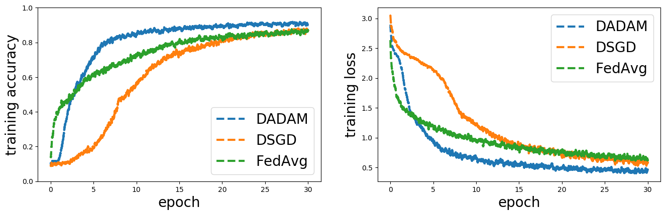
Figure 1: Convergence of different stochastic algorithms over 100 epochs on the datasets from SGDLibrary [51]. (left) fixed step-size and (right) diminishing step-size.The legend for all curves is on the top right.

Refer to caption

Figure 2: Training simple MLP on the MNIST digit recognition dataset. Training loss and accuracy of different distributed algorithms over 30 epochs.

Acknowledgements

The second author is grateful for a discussion of decentralized methods with Davood Hajinezhad.

References

  • [1] S. Shalev-Shwartz et al., “Online learning and online convex optimization,” Foundations and Trends® in Machine Learning, vol. 4, no. 2, pp. 107–194, 2012.
  • [2] E. Hazan et al., “Introduction to online convex optimization,” Foundations and Trends® in Optimization, vol. 2, no. 3-4, pp. 157–325, 2016.
  • [3] M. Zinkevich, “Online convex programming and generalized infinitesimal gradient ascent,” 2003.
  • [4] E. C. Hall and R. M. Willett, “Online convex optimization in dynamic environments,” IEEE Journal of Selected Topics in Signal Processing, vol. 9, no. 4, pp. 647–662, 2015.
  • [5] O. Besbes, Y. Gur, and A. Zeevi, “Non-stationary stochastic optimization,” Operations Research, vol. 63, no. 5, pp. 1227–1244, 2015.
  • [6] S. Shahrampour and A. Jadbabaie, “Distributed online optimization in dynamic environments using mirror descent,” IEEE Transactions on Automatic Control, vol. 63, no. 3, pp. 714–725, 2018.
  • [7] A. Mokhtari, S. Shahrampour, A. Jadbabaie, and A. Ribeiro, “Online optimization in dynamic environments: Improved regret rates for strongly convex problems,” in Decision and Control (CDC), 2016 IEEE 55th Conference on, pp. 7195–7201, IEEE, 2016.
  • [8] L. Zhang, T. Yang, J. Yi, J. Rong, and Z.-H. Zhou, “Improved dynamic regret for non-degenerate functions,” in Advances in Neural Information Processing Systems, pp. 732–741, 2017.
  • [9] J. Tsitsiklis, D. Bertsekas, and M. Athans, “Distributed asynchronous deterministic and stochastic gradient optimization algorithms,” IEEE transactions on automatic control, vol. 31, no. 9, pp. 803–812, 1986.
  • [10] D. Li, K. D. Wong, Y. H. Hu, and A. M. Sayeed, “Detection, classification, and tracking of targets,” IEEE signal processing magazine, vol. 19, no. 2, pp. 17–29, 2002.
  • [11] M. Rabbat and R. Nowak, “Distributed optimization in sensor networks,” in Proceedings of the 3rd international symposium on Information processing in sensor networks, pp. 20–27, ACM, 2004.
  • [12] V. Lesser, C. L. Ortiz Jr, and M. Tambe, Distributed sensor networks: A multiagent perspective, vol. 9. Springer Science & Business Media, 2012.
  • [13] A. Nedic and A. Ozdaglar, “Distributed subgradient methods for multi-agent optimization,” IEEE Transactions on Automatic Control, vol. 54, no. 1, pp. 48–61, 2009.
  • [14] J. C. Duchi, A. Agarwal, and M. J. Wainwright, “Dual averaging for distributed optimization: Convergence analysis and network scaling,” IEEE Transactions on Automatic control, vol. 57, no. 3, pp. 592–606, 2012.
  • [15] K. Yuan, Q. Ling, and W. Yin, “On the convergence of decentralized gradient descent,” SIAM Journal on Optimization, vol. 26, no. 3, pp. 1835–1854, 2016.
  • [16] J. Zeng and W. Yin, “On nonconvex decentralized gradient descent,” IEEE Transactions on Signal Processing, vol. 66, no. 11, pp. 2834–2848, 2018.
  • [17] W. Shi, Q. Ling, G. Wu, and W. Yin, “Extra: An exact first-order algorithm for decentralized consensus optimization,” SIAM Journal on Optimization, vol. 25, no. 2, pp. 944–966, 2015.
  • [18] A. Nedic, A. Olshevsky, and W. Shi, “Achieving geometric convergence for distributed optimization over time-varying graphs,” SIAM Journal on Optimization, vol. 27, no. 4, pp. 2597–2633, 2017.
  • [19] H. Tang, X. Lian, M. Yan, C. Zhang, and J. Liu, “D2: Decentralized training over decentralized data,” arXiv preprint arXiv:1803.07068, 2018.
  • [20] Z. Jiang, A. Balu, C. Hegde, and S. Sarkar, “Collaborative deep learning in fixed topology networks,” in Advances in Neural Information Processing Systems, pp. 5904–5914, 2017.
  • [21] T.-H. Chang, A. Nedić, and A. Scaglione, “Distributed constrained optimization by consensus-based primal-dual perturbation method,” IEEE Transactions on Automatic Control, vol. 59, no. 6, pp. 1524–1538, 2014.
  • [22] G. Lan, S. Lee, and Y. Zhou, “Communication-efficient algorithms for decentralized and stochastic optimization,” arXiv preprint arXiv:1701.03961, 2017.
  • [23] E. Wei and A. Ozdaglar, “Distributed alternating direction method of multipliers,” 2012.
  • [24] W. Shi, Q. Ling, K. Yuan, G. Wu, and W. Yin, “On the linear convergence of the admm in decentralized consensus optimization,” IEEE Transactions on Signal Processing, vol. 62, pp. 1750–1761, 2014.
  • [25] D. Hajinezhad, M. Hong, and A. Garcia, “Zeroth order nonconvex multi-agent optimization over networks,” arXiv preprint arXiv:1710.09997, 2017.
  • [26] X. Lian, C. Zhang, H. Zhang, C.-J. Hsieh, W. Zhang, and J. Liu, “Can decentralized algorithms outperform centralized algorithms? a case study for decentralized parallel stochastic gradient descent,” in Advances in Neural Information Processing Systems, pp. 5330–5340, 2017.
  • [27] J. Duchi, E. Hazan, and Y. Singer, “Adaptive subgradient methods for online learning and stochastic optimization,” Journal of Machine Learning Research, vol. 12, no. Jul, pp. 2121–2159, 2011.
  • [28] D. Kingma and J. Ba, “Adam: A method for stochastic optimization,” arXiv preprint arXiv:1412.6980, 2014.
  • [29] T. Tieleman and G. Hinton, “Divide the gradient by a running average of its recent magnitude. coursera: Neural networks for machine learning,” tech. rep., Technical Report. Available online: https://zh. coursera. org/learn/neuralnetworks/lecture/YQHki/rmsprop-divide-the-gradient-by-a-running-average-of-its-recent-magnitude (accessed on 21 April 2017).
  • [30] X. Zhang, J. Zhang, and L. Liao, “An adaptive trust region method and its convergence,” Science in China Series A: Mathematics, vol. 45, no. 5, pp. 620–631, 2002.
  • [31] D. Ataee Tarzanagh, M. R. Peyghami, and H. Mesgarani, “A new nonmonotone trust region method for unconstrained optimization equipped by an efficient adaptive radius,” Optimization Methods and Software, vol. 29, no. 4, pp. 819–836, 2014.
  • [32] D. A. Tarzanagh, M. R. Peyghami, and F. Bastin, “A new nonmonotone adaptive retrospective trust region method for unconstrained optimization problems,” Journal of Optimization Theory and Applications, vol. 167, no. 2, pp. 676–692, 2015.
  • [33] M. D. Zeiler, “Adadelta: an adaptive learning rate method,” arXiv preprint arXiv:1212.5701, 2012.
  • [34] S. J. Reddi, S. Kale, and S. Kumar, “On the convergence of adam and beyond,” in International Conference on Learning Representations, 2018.
  • [35] A. C. Wilson, R. Roelofs, M. Stern, N. Srebro, and B. Recht, “The marginal value of adaptive gradient methods in machine learning,” in Advances in Neural Information Processing Systems, pp. 4148–4158, 2017.
  • [36] D. Zhou, Y. Tang, Z. Yang, Y. Cao, and Q. Gu, “On the convergence of adaptive gradient methods for nonconvex optimization,” arXiv preprint arXiv:1808.05671, 2018.
  • [37] X. Chen, S. Liu, R. Sun, and M. Hong, “On the convergence of a class of adam-type algorithms for non-convex optimization,” arXiv preprint arXiv:1808.02941, 2018.
  • [38] R. Ward, X. Wu, and L. Bottou, “Adagrad stepsizes: Sharp convergence over nonconvex landscapes, from any initialization,” arXiv preprint arXiv:1806.01811, 2018.
  • [39] S. De, A. Mukherjee, and E. Ullah, “Convergence guarantees for rmsprop and adam in non-convex optimization and an empirical comparison to nesterov acceleration,” 2018.
  • [40] A. Basu, S. De, A. Mukherjee, and E. Ullah, “Convergence guarantees for rmsprop and adam in non-convex optimization and their comparison to nesterov acceleration on autoencoders,” arXiv preprint arXiv:1807.06766, 2018.
  • [41] M. Zaheer, S. Reddi, D. Sachan, S. Kale, and S. Kumar, “Adaptive methods for nonconvex optimization,” in Advances in Neural Information Processing Systems, pp. 9815–9825, 2018.
  • [42] H. B. McMahan and M. Streeter, “Adaptive bound optimization for online convex optimization,” arXiv preprint arXiv:1002.4908, 2010.
  • [43] J. Dean, G. Corrado, R. Monga, K. Chen, M. Devin, M. Mao, A. Senior, P. Tucker, K. Yang, Q. V. Le, et al., “Large scale distributed deep networks,” in Advances in neural information processing systems, pp. 1223–1231, 2012.
  • [44] M. Li, D. G. Andersen, J. W. Park, A. J. Smola, A. Ahmed, V. Josifovski, J. Long, E. J. Shekita, and B.-Y. Su, “Scaling distributed machine learning with the parameter server.,” in OSDI, vol. 14, pp. 583–598, 2014.
  • [45] D. Mateos-Núnez and J. Cortés, “Distributed online convex optimization over jointly connected digraphs,” IEEE Transactions on Network Science and Engineering, vol. 1, no. 1, pp. 23–37, 2014.
  • [46] E. Hazan, K. Singh, and C. Zhang, “Efficient regret minimization in non-convex games,” arXiv preprint arXiv:1708.00075, 2017.
  • [47] A. Nedić, A. Olshevsky, and M. G. Rabbat, “Network topology and communication-computation tradeoffs in decentralized optimization,” Proceedings of the IEEE, vol. 106, no. 5, pp. 953–976, 2018.
  • [48] H. Robbins and S. Monro, “A stochastic approximation method,” in Herbert Robbins Selected Papers, pp. 102–109, Springer, 1985.
  • [49] S. Boyd, P. Diaconis, and L. Xiao, “Fastest mixing markov chain on a graph,” SIAM review, vol. 46, no. 4, pp. 667–689, 2004.
  • [50] H. B. McMahan, E. Moore, D. Ramage, S. Hampson, et al., “Communication-efficient learning of deep networks from decentralized data,” arXiv preprint arXiv:1602.05629, 2016.
  • [51] H. Kasai, “Sgdlibrary: A matlab library for stochastic optimization algorithms,” Journal of Machine Learning Research, vol. 18, no. 215, pp. 1–5, 2018.
  • [52] A. Beck and M. Teboulle, “Mirror descent and nonlinear projected subgradient methods for convex optimization,” Operations Research Letters, vol. 31, no. 3, pp. 167–175, 2003.
  • [53] S. Shahrampour and A. Jadbabaie, “An online optimization approach for multi-agent tracking of dynamic parameters in the presence of adversarial noise,” in American Control Conference (ACC), 2017, pp. 3306–3311, IEEE, 2017.
  • [54] R. A. Horn, R. A. Horn, and C. R. Johnson, Matrix analysis. Cambridge university press, 1990.
  • [55] H. Attouch, J. Bolte, and B. F. Svaiter, “Convergence of descent methods for semi-algebraic and tame problems: proximal algorithms, forward–backward splitting, and regularized gauss–seidel methods,” Mathematical Programming, vol. 137, no. 1-2, pp. 91–129, 2013.

7 Supplementary Material

Next, we establish a series of lemmas used in the proof of main theorems.

7.1 Auxiliary Lemmas

Lemma 12.

[52] Let 𝒳\mathcal{X} be a nonempty closed convex set in ℝp\mathbb{R}^{p}. Then, for any d∈𝒳d\in\mathcal{X}, we have

⟨x∗−d,a⟩≤12​‖d−c‖2−12​‖d−x∗‖2−12​‖x∗−c‖2,\langle x^{*}-d,a\rangle\leq\frac{1}{2}\|d-c\|^{2}-\frac{1}{2}\|d-x^{*}\|^{2}-\frac{1}{2}\|x^{*}-c\|^{2},

where

x∗=arg​minx∈𝒳⁡{⟨a,x⟩+12​‖x−c‖2}.x^{*}=\argmin_{x\in\mathcal{X}}\{\langle a,x\rangle+\frac{1}{2}\|x-c\|^{2}\}.
Lemma 13.

[42] For any A∈𝒮+pA\in\mathcal{S}^{p}_{+} and convex feasible set C⊂ℝp,C\subset\mathbb{R}^{p}, suppose a1=ΠC,A​[b1],a2=ΠC,A​[b2]a_{1}=\Pi_{C,A}[b_{1}],a_{2}=\Pi_{C,A}[b_{2}]. Then, we have

‖A12​(a1−a2)‖≤‖A12​(b1−b2)‖.\|A^{\frac{1}{2}}(a_{1}-a_{2})\|\leq\|A^{\frac{1}{2}}(b_{1}-b_{2})\|.
Lemma 14.

Let β1,β2∈[0,1)\beta_{1},\beta_{2}\in[0,1) satisfy η=β1β2<1\eta=\frac{\beta_{1}}{\sqrt{\beta_{2}}}<1. Then, for any i∈𝒱i\in\mathcal{V}, we have

∑t=1T∑d=1pαt​mi,t,d2υ^i,t,d≤α​1+log⁡T(1−β1)​(1−η)​(1−β2)​(1−β3)∑d=1p∥gi,1:T,d∥,\sum_{t=1}^{T}\sum_{d=1}^{p}\frac{\alpha_{t}m^{2}_{i,t,d}}{\sqrt{\widehat{\upsilon}_{i,t,d}}}\leq\frac{\alpha\sqrt{1+\log T}}{(1-\beta_{1})(1-\eta)\sqrt{(1-\beta_{2})(1-\beta_{3})}}\sum_{d=1}^{p}\|g_{i,1:T,d}\|,

where αt=αt\alpha_{t}=\frac{\alpha}{\sqrt{t}} for all t∈{1,…,T}t\in\{1,\dots,T\}.

Proof.

Using the update rule of moment vectors mi,tm_{i,t} and υ^i,t\widehat{\upsilon}_{i,t} in Algorithm 1, we have

∑t=1Tα​mi,t,d2t​υ^i,t,d\displaystyle\sum_{t=1}^{T}\frac{\alpha m^{2}_{i,t,d}}{\sqrt{t\widehat{\upsilon}_{i,t,d}}} =∑t=1T−1α​mi,t,d2t​υ^i,t,d+αT​mi,T,d2(1−β3)​max⁡{υ^i,T−1,d,υi,T,d}+β3​υ^i,T−1,d\displaystyle=\sum_{t=1}^{T-1}\frac{\alpha m^{2}_{i,t,d}}{\sqrt{t\widehat{\upsilon}_{i,t,d}}}+\frac{\alpha_{T}m^{2}_{i,T,d}}{\sqrt{(1-\beta_{3})\max\{\widehat{\upsilon}_{i,T-1,d},\upsilon_{i,T,d}\}+\beta_{3}\widehat{\upsilon}_{i,T-1,d}}}
≤∑t=1T−1α​mi,t,d2t​υ^i,t,d+αT​mi,T,d2(1−β3)​υi,T,d\displaystyle\leq\sum_{t=1}^{T-1}\frac{\alpha m^{2}_{i,t,d}}{\sqrt{t\widehat{\upsilon}_{i,t,d}}}+\frac{\alpha_{T}m^{2}_{i,T,d}}{\sqrt{(1-\beta_{3})\upsilon_{i,T,d}}}
=∑t=1T−1α​mi,t,d2t​υ^i,t,d+α​(∑l=1T(1−β1)​β1T−l​gi,l,d)2(1−β3)​T​∑l=1T(1−β2)​β2T−l​gi,l,d2\displaystyle\mathrel{{\mathop{=}\limits}}\sum_{t=1}^{T-1}\frac{\alpha m^{2}_{i,t,d}}{\sqrt{t\widehat{\upsilon}_{i,t,d}}}+\frac{\alpha(\sum_{l=1}^{T}(1-\beta_{1})\beta_{1}^{T-l}g_{i,l,d})^{2}}{\sqrt{(1-\beta_{3})T\sum_{l=1}^{T}(1-\beta_{2})\beta_{2}^{T-l}g^{2}_{i,l,d}}}
≤∑t=1T−1α​mi,t,d2t​υ^i,t,d+αT⁡(1−β2)​(1−β3)​(∑l=1Tβ1T−l)​(∑l=1Tβ1T−l​gi,l,d2)∑l=1Tβ2T−l​gi,l,d2\displaystyle\mathrel{{\mathop{\leq}\limits}}\sum_{t=1}^{T-1}\frac{\alpha m^{2}_{i,t,d}}{\sqrt{t\widehat{\upsilon}_{i,t,d}}}+\frac{\alpha}{\sqrt{T(1-\beta_{2})(1-\beta_{3})}}\frac{(\sum_{l=1}^{T}\beta_{1}^{T-l})(\sum_{l=1}^{T}\beta_{1}^{T-l}g^{2}_{i,l,d})}{\sqrt{\sum_{l=1}^{T}\beta_{2}^{T-l}g^{2}_{i,l,d}}}
≤∑t=1T−1α​mi,t,d2t​υ^i,t,d+α(1−β1)​T⁡(1−β2)​(1−β3)​∑l=1Tβ1T−l​gi,l,d2β2T−l​gi,l,d2\displaystyle\mathrel{{\mathop{\leq}\limits}}\sum_{t=1}^{T-1}\frac{\alpha m^{2}_{i,t,d}}{\sqrt{t\widehat{\upsilon}_{i,t,d}}}+\frac{\alpha}{(1-\beta_{1})\sqrt{T(1-\beta_{2})(1-\beta_{3})}}\sum_{l=1}^{T}\frac{\beta_{1}^{T-l}g^{2}_{i,l,d}}{\sqrt{\beta_{2}^{T-l}g^{2}_{i,l,d}}}
≤∑t=1T−1α​mi,t,d2t​υ^i,t,d+α(1−β1)​T⁡(1−β2)​(1−β3)​∑l=1TηT−l​|gi,l,d|,\displaystyle{\leq}\sum_{t=1}^{T-1}\frac{\alpha m^{2}_{i,t,d}}{\sqrt{t\widehat{\upsilon}_{i,t,d}}}+\frac{\alpha}{(1-\beta_{1})\sqrt{T(1-\beta_{2})(1-\beta_{3})}}\sum_{l=1}^{T}\eta^{T-l}|g_{i,l,d}|,

where (i) follows from the fact that the update rules of mTm_{T} and υT\upsilon_{T} can be written as mT=(1−β1)​∑l=1Tβ1T−l​glm_{T}=(1-\beta_{1})\sum_{l=1}^{T}\beta_{1}^{T-l}g_{l} and υT=(1−β2)​∑l=1Tβ2T−l​gl2\upsilon_{T}=(1-\beta_{2})\sum_{l=1}^{T}\beta_{2}^{T-l}g_{l}^{2}, respectively. (ii) follows from Cauchy-Schwarz inequality and the fact that 0≤β1<10\leq\beta_{1}<1. Inequality (iii) follows since ∑l=1Tβ1T−l≤11−β1\sum_{l=1}^{T}\beta_{1}^{T-l}\leq\frac{1}{1-\beta_{1}}. Hence, we have

∑t=1Tα​mi,t,d2(1−β1)​t​υ^i,t,d\displaystyle\sum_{t=1}^{T}\frac{\alpha m^{2}_{i,t,d}}{(1-\beta_{1})\sqrt{t\widehat{\upsilon}_{i,t,d}}} ≤∑t=1Tα(1−β1)​t⁡(1−β2)​(1−β3)​∑l=1tηt−l​|gi,l,d|\displaystyle\leq\sum_{t=1}^{T}\frac{\alpha}{(1-\beta_{1})\sqrt{t(1-\beta_{2})(1-\beta_{3})}}\sum_{l=1}^{t}\eta^{t-l}|g_{i,l,d}|
=α(1−β1)​(1−β2)​(1−β3)​∑t=1T1t​∑l=1tηt−l​|gi,l,d|\displaystyle=\frac{\alpha}{(1-\beta_{1})\sqrt{(1-\beta_{2})(1-\beta_{3})}}\sum_{t=1}^{T}\frac{1}{\sqrt{t}}\sum_{l=1}^{t}\eta^{t-l}|g_{i,l,d}|
=α(1−β1)​(1−β2)​(1−β3)​∑t=1T|gi,t,d|​∑l=tTηl−tl\displaystyle=\frac{\alpha}{(1-\beta_{1})\sqrt{(1-\beta_{2})(1-\beta_{3})}}\sum_{t=1}^{T}|g_{i,t,d}|\sum_{l=t}^{T}\frac{\eta^{l-t}}{\sqrt{l}}
≤α(1−β1)​(1−β2)​(1−β3)​∑t=1T|gi,t,d|​∑l=tTηl−tt\displaystyle{\leq}\frac{\alpha}{(1-\beta_{1})\sqrt{(1-\beta_{2})(1-\beta_{3})}}\sum_{t=1}^{T}|g_{i,t,d}|\sum_{l=t}^{T}\frac{\eta^{l-t}}{\sqrt{t}}
≤α(1−β1)​(1−β2)​(1−β3)​∑t=1T|gi,t,d|​1(1−η)​t\displaystyle\mathrel{{\mathop{\leq}\limits}}\frac{\alpha}{(1-\beta_{1})\sqrt{(1-\beta_{2})(1-\beta_{3})}}\sum_{t=1}^{T}|g_{i,t,d}|\frac{1}{(1-\eta)\sqrt{t}}
≤α(1−β1)​(1−η)​(1−β2)​(1−β3)∥gi,1:T,d∥∑t=1T1t\displaystyle\mathrel{{\mathop{\leq}\limits}}\frac{\alpha}{(1-\beta_{1})(1-\eta)\sqrt{(1-\beta_{2})(1-\beta_{3})}}\|g_{i,1:T,d}\|\sqrt{\sum_{t=1}^{T}\frac{1}{t}}
≤α​1+log⁡T(1−β1)​(1−η)​(1−β2)​(1−β3)∥gi,1:T,d∥,\displaystyle\mathrel{{\mathop{\leq}\limits}}\frac{\alpha\sqrt{1+\log T}}{(1-\beta_{1})(1-\eta)\sqrt{(1-\beta_{2})(1-\beta_{3})}}\|g_{i,1:T,d}\|,

where inequality (i) follows since ∑l=tTηl−t≤1(1−η)\sum_{l=t}^{T}\eta^{l-t}\leq\frac{1}{(1-\eta)}. Inequality (ii) follows from Cauchy-Schwarz inequality. The inequality (iii) follows since

∑t=1T1t≤1+∫t=1T1t​𝑑t=1+log⁡t|1T=1+log⁡T.\sum_{t=1}^{T}\frac{1}{t}\leq 1+\int_{t=1}^{T}\frac{1}{t}dt=1+\log t|_{1}^{T}=1+\log T. (17)

∎

Next, we provide an upper bound on the deviation of the local estimates at each iteration from their consensual value. A similar result has been proven in [53] for online decentralized mirror descent; however, the following lemma extends that of [53] to the online adaptive setting and takes into account the sparsity of gradient vector.

Lemma 15 (Network Error with Sparse Data).

Suppose Assumption 2 holds. If β1,β2∈[0,1)\beta_{1},\beta_{2}\in[0,1) satisfy η=β1β2<1\eta=\frac{\beta_{1}}{\sqrt{\beta_{2}}}<1, then the sequence xi,tx_{i,t} generated by Algorithm 1 satisfies

∑t=1T∑i=1n1αt∥V^i,t14(x¯t−xi,t)∥2≤nnα1+log⁡T∑d=1p∥g1:T,d∥(1−σ2​(W))2​(1−β1)​(1−η)​(1−β2)​(1−β3),\sum_{t=1}^{T}\sum_{i=1}^{n}\frac{1}{\alpha_{t}}\|{\widehat{V}_{i,t}}^{\frac{1}{4}}(\bar{x}_{t}-x_{i,t})\|^{2}\leq\frac{n\sqrt{n}\alpha\sqrt{1+\log T}\sum_{d=1}^{p}\|g_{1:T,d}\|}{(1-\sigma_{2}(W))^{2}(1-\beta_{1})(1-\eta)\sqrt{(1-\beta_{2})(1-\beta_{3})}},

where V^i,t=diag​(υ^i,t)\widehat{V}_{i,t}=\text{diag}(\widehat{\upsilon}_{i,t}) and x¯t=1n​∑i=1nxi,t.\bar{x}_{t}=\frac{1}{n}\sum_{i=1}^{n}x_{i,t}.

Proof.

Let ei,t:=xi,t+1−∑j=1n[W]i​j​xj,te_{i,t}:=x_{i,t+1}-\sum_{j=1}^{n}[W]_{ij}x_{j,t}, where WW satisfies (6). Using the update rule of xi,t+1x_{i,t+1} in Algorithm 1, we have

∑t=1T1αt​‖V^i,t14​ei,t‖2\displaystyle\sum_{t=1}^{T}\frac{1}{\alpha_{t}}\|\widehat{V}_{i,t}^{\frac{1}{4}}e_{i,t}\|^{2} =∑t=1T1αt​‖V^i,t14​(xi,t+1−∑j=1n[W]i​j​xj,t)‖2\displaystyle=\sum_{t=1}^{T}\frac{1}{\alpha_{t}}\|\widehat{V}_{i,t}^{\frac{1}{4}}(x_{i,t+1}-\sum_{j=1}^{n}[W]_{ij}x_{j,t})\|^{2}
=∑t=1T1αt​‖V^i,t14​(Π𝒳,V^i,t​[∑j=1n[W]i​j​xj,t−αt​mi,tυ^i,t]−∑j=1n[W]i​j​xj,t)‖2\displaystyle=\sum_{t=1}^{T}\frac{1}{\alpha_{t}}\|\widehat{V}_{i,t}^{\frac{1}{4}}(\Pi_{\mathcal{X},\sqrt{\widehat{V}_{i,t}}}\big[\sum_{j=1}^{n}[W]_{ij}x_{j,t}-\frac{\alpha_{t}m_{i,t}}{\sqrt{\widehat{\upsilon}_{i,t}}}\big]-\sum_{j=1}^{n}[W]_{ij}x_{j,t})\|^{2}
≤∑t=1T1αt​‖V^i,t14​(∑j=1n[W]i​j​xj,t−αt​V^i,t−12​mi,t−∑j=1n[W]i​j​xj,t)‖2\displaystyle\leq\sum_{t=1}^{T}\frac{1}{\alpha_{t}}\|\widehat{V}_{i,t}^{\frac{1}{4}}(\sum_{j=1}^{n}[W]_{ij}x_{j,t}-\alpha_{t}\widehat{V}_{i,t}^{\frac{-1}{2}}m_{i,t}-\sum_{j=1}^{n}[W]_{ij}x_{j,t})\|^{2}
=∑t=1T∑d=1pαt​mi,t,d2υ^i,t,d,\displaystyle=\sum_{t=1}^{T}\sum_{d=1}^{p}\frac{\alpha_{t}m^{2}_{i,t,d}}{\sqrt{\widehat{\upsilon}_{i,t,d}}}, (18)

where the first inequality follows from Lemma 13.

Further, from the definition of ei,te_{i,t}, we have

xi,t+1=∑j=1n[W]i​j​xj,t+ei,t.x_{i,t+1}=\sum_{j=1}^{n}[W]_{ij}x_{j,t}+e_{i,t}. (19)

Now, from (6) and (19), we have

x¯t+1=1n​∑i=1nxi,t+1\displaystyle\bar{x}_{t+1}=\frac{1}{n}\sum_{i=1}^{n}x_{i,t+1} =1n​∑i=1n∑j=1n[W]i​j​xj,t+1n​∑i=1nei,t\displaystyle=\frac{1}{n}\sum_{i=1}^{n}\sum_{j=1}^{n}[W]_{ij}x_{j,t}+\frac{1}{n}\sum_{i=1}^{n}e_{i,t}
=1n​∑j=1n(∑i=1n[W]i​j)​xj,t+1n​∑i=1nei,t\displaystyle=\frac{1}{n}\sum_{j=1}^{n}(\sum_{i=1}^{n}[W]_{ij})x_{j,t}+\frac{1}{n}\sum_{i=1}^{n}e_{i,t}
=x¯t+e¯t,\displaystyle=\bar{x}_{t}+\bar{e}_{t},

where e¯t=1n​∑i=1nei,t\bar{e}_{t}=\frac{1}{n}\sum_{i=1}^{n}e_{i,t}. Hence,

x¯t+1=∑s=0te¯s.\bar{x}_{t+1}=\sum_{s=0}^{t}\bar{e}_{s}. (20)

It follows from (19) that

xi,t+1=∑s=0t∑j=1n[Wt−s]i​j​ei,s.x_{i,t+1}=\sum_{s=0}^{t}\sum_{j=1}^{n}[W^{t-s}]_{ij}e_{i,s}. (21)

Now, using (21) and (20), we have

xi,t+1−x¯t+1=∑s=0t∑j=1n([Wt−s]i​j−1n)​ei,s.x_{i,t+1}-\bar{x}_{t+1}=\sum_{s=0}^{t}\sum_{j=1}^{n}([W^{t-s}]_{ij}-\frac{1}{n})e_{i,s}. (22)

Now, taking the Euclidean norm of (22) and summing over t∈{1,…,T}t\in\{1,\ldots,T\}, one has:

∑t=1T1αt​‖V^i,t14​(xi,t+1−x¯t+1)‖2\displaystyle\sum_{t=1}^{T}\frac{1}{\alpha_{t}}\|\widehat{V}_{i,t}^{\frac{1}{4}}(x_{i,t+1}-\bar{x}_{t+1})\|^{2} ≤∑t=1Tt​∑s=0t(∑j=1n|[Wt−s]i​j−1n|)2​‖V^i,s14​ei,s‖2αs\displaystyle\mathrel{{\mathop{\leq}\limits}}\sum_{t=1}^{T}t\sum_{s=0}^{t}(\sum_{j=1}^{n}|[W^{t-s}]_{ij}-\frac{1}{n}|)^{2}\frac{\|\widehat{V}_{i,s}^{\frac{1}{4}}e_{i,s}\|^{2}}{\alpha_{s}}
≤∑s=0T‖V^i,s14​ei,s‖2αs​∑t=1Tn​t​σ22​t−2​s​(W)\displaystyle\mathrel{{\mathop{\leq}\limits}}\sum_{s=0}^{T}\frac{\|\widehat{V}_{i,s}^{\frac{1}{4}}e_{i,s}\|^{2}}{\alpha_{s}}\sum_{t=1}^{T}nt\sigma^{2t-2s}_{2}(W)
≤n(1−σ2​(W))2​∑t=0T‖V^i,t14​ei,t‖2αt\displaystyle\mathrel{{\mathop{\leq}\limits}}\frac{n}{(1-\sigma_{2}(W))^{2}}\sum_{t=0}^{T}\frac{\|\widehat{V}_{i,t}^{\frac{1}{4}}e_{i,t}\|^{2}}{\alpha_{t}}
≤n(1−σ2​(W))2​∑d=1p∑t=1Tαt​mi,t,d2υ^i,t,d\displaystyle\mathrel{{\mathop{\leq}\limits}}\frac{n}{(1-\sigma_{2}(W))^{2}}\sum_{d=1}^{p}\sum_{t=1}^{T}\frac{\alpha_{t}m^{2}_{i,t,d}}{\sqrt{\widehat{\upsilon}_{i,t,d}}}
≤nα1+log⁡T∑d=1p∥gi,1:T,d∥(1−σ2​(W))2​(1−β1)​(1−η)​(1−β2)​(1−β3),\displaystyle\mathrel{{\mathop{\leq}\limits}}\frac{n\alpha\sqrt{1+\log T}\sum_{d=1}^{p}\|g_{i,1:T,d}\|}{(1-\sigma_{2}(W))^{2}(1-\beta_{1})(1-\eta)\sqrt{(1-\beta_{2})(1-\beta_{3})}}, (23)

where step (i) follows from ‖∑i=1nai‖2≤n​∑i=1n‖ai‖2\|\sum_{i=1}^{n}a_{i}\|^{2}\leq n\sum_{i=1}^{n}\|a_{i}\|^{2}, step (ii) follows from the following property of mixing matrix WW [54],

∑j=1n|[Wt]i​j−1n|≤n​σ2t​(W),\sum_{j=1}^{n}\left|\left[W^{t}\right]_{ij}-\frac{1}{n}\right|\leq\sqrt{n}\sigma^{t}_{2}(W), (24)

step (iii) follows from ∑t=1Tt​σ2t​(W)<1(1−σ2​(W))2\sum_{t=1}^{T}t\sigma^{t}_{2}(W)<\frac{1}{(1-\sigma_{2}(W))^{2}}, step (iv) follows from (7.1) and step (v) follows from Lemma 14.

Now, summing (7.1) over i∈𝒱i\in\mathcal{V} and using

∑i=1n∥gi,1:T,d∥≤n(∑i=1n∥gi,1:T,d∥2)12=n∥g1:T,d∥,\sum_{i=1}^{n}\|g_{i,1:T,d}\|\leq\sqrt{n}(\sum_{i=1}^{n}\|g_{i,1:T,d}\|^{2})^{\frac{1}{2}}=\sqrt{n}\|g_{1:T,d}\|, (25)

we complete the proof. ∎

Lemma 16.

For the sequence xi,tx_{i,t} generated by Algorithm 1 and the parameter settings and conditions assumed in Theorem 5, we have

1n​∑i=1n∑t=1T(υ^i,tαt​(1−β1,t)​‖xt∗−∑j=1n[W]i​j​xj,t‖2−υ^i,tαt​(1−β1,t)​‖xt∗−xi,t+1‖2)\displaystyle\frac{1}{n}\sum_{i=1}^{n}\sum_{t=1}^{T}(\frac{\sqrt{\widehat{\upsilon}_{i,t}}}{\alpha_{t}(1-\beta_{1,t})}\|x^{*}_{t}-\sum_{j=1}^{n}[W]_{ij}x_{j,t}\|^{2}-\frac{\sqrt{\widehat{\upsilon}_{i,t}}}{\alpha_{t}(1-\beta_{1,t})}\|x^{*}_{t}-x_{i,t+1}\|^{2})
≤2​γ∞2n​(1−β1)​∑d=1pυ^T,dαT+2​γ∞n​∑d=1pυ^T,dαT​(1−β1)​∑t=1T−1|xt+1,d∗−xt,d∗|+γ∞2​G∞α​(1−λ)2​(1−β1)2.\displaystyle\leq\frac{2\gamma_{\infty}^{2}}{\sqrt{n}(1-\beta_{1})}\sum_{d=1}^{p}\frac{\sqrt{\widehat{\upsilon}_{T,d}}}{\alpha_{T}}+\frac{2\gamma_{\infty}}{\sqrt{n}}\sum_{d=1}^{p}\frac{\sqrt{\widehat{\upsilon}_{T,d}}}{\alpha_{T}(1-\beta_{1})}\sum_{t=1}^{T-1}|x^{*}_{t+1,d}-x^{*}_{t,d}|+\frac{\gamma_{\infty}^{2}G_{\infty}}{\alpha(1-\lambda)^{2}(1-\beta_{1})^{2}}. (26)
Proof.

From the left side of (16), we have

υ^i,tαt​(1−β1,t)​‖xt∗−∑j=1n[W]i​j​xj,t‖2−υ^i,tαt​(1−β1,t)​‖xt∗−xi,t+1‖2\displaystyle\frac{\sqrt{\widehat{\upsilon}_{i,t}}}{\alpha_{t}(1-\beta_{1,t})}\|x^{*}_{t}-\sum_{j=1}^{n}[W]_{ij}x_{j,t}\|^{2}-\frac{\sqrt{\widehat{\upsilon}_{i,t}}}{\alpha_{t}(1-\beta_{1,t})}\|x^{*}_{t}-x_{i,t+1}\|^{2}
=υ^i,tαt​(1−β1,t)​‖xt∗−∑j=1n[W]i​j​xj,t‖2−υ^i,t+1αt+1​(1−β1,t+1)​‖xt+1∗−∑j=1n[W]i​j​xj,t+1‖2\displaystyle=\frac{\sqrt{\widehat{\upsilon}_{i,t}}}{\alpha_{t}(1-\beta_{1,t})}\|x^{*}_{t}-\sum_{j=1}^{n}[W]_{ij}x_{j,t}\|^{2}-\frac{\sqrt{\widehat{\upsilon}_{i,t+1}}}{\alpha_{t+1}(1-\beta_{1,t+1})}\|x^{*}_{t+1}-\sum_{j=1}^{n}[W]_{ij}x_{j,t+1}\|^{2}
+υ^i,t+1αt+1​(1−β1,t+1)​‖xt+1∗−∑j=1n[W]i​j​xj,t+1‖2−υ^i,t+1αt+1​(1−β1,t+1)​‖xt∗−∑j=1n[W]i​j​xj,t+1‖2\displaystyle+\frac{\sqrt{\widehat{\upsilon}_{i,t+1}}}{\alpha_{t+1}(1-\beta_{1,t+1})}\|x^{*}_{t+1}-\sum_{j=1}^{n}[W]_{ij}x_{j,t+1}\|^{2}-\frac{\sqrt{\widehat{\upsilon}_{i,t+1}}}{\alpha_{t+1}(1-\beta_{1,t+1})}\|x^{*}_{t}-\sum_{j=1}^{n}[W]_{ij}x_{j,t+1}\|^{2} (27)
+υ^i,t+1αt+1​(1−β1,t+1)​‖xt∗−xi,t+1‖2−υ^i,tαt​(1−β1,t)​‖xt∗−xi,t+1‖2⏟I1.\displaystyle+\underbrace{\frac{\sqrt{\widehat{\upsilon}_{i,t+1}}}{\alpha_{t+1}(1-\beta_{1,t+1})}\|x^{*}_{t}-x_{i,t+1}\|^{2}-\frac{\sqrt{\widehat{\upsilon}_{i,t}}}{\alpha_{t}(1-\beta_{1,t})}\|x^{*}_{t}-x_{i,t+1}\|^{2}}_{I_{1}}. (28)

By construction of (27), we have

υ^i,t+1​‖xt+1∗−∑j=1n[W]i​j​xj,t+1‖2−υ^i,t+1​‖xt∗−∑j=1n[W]i​j​xj,t+1‖2\displaystyle\sqrt{\widehat{\upsilon}_{i,t+1}}\|x^{*}_{t+1}-\sum_{j=1}^{n}[W]_{ij}x_{j,t+1}\|^{2}-\sqrt{\widehat{\upsilon}_{i,t+1}}\|x^{*}_{t}-\sum_{j=1}^{n}[W]_{ij}x_{j,t+1}\|^{2}
=∑d=1pυ^i,t+1,d​⟨xt+1,d∗−xt,d∗,xt+1,d∗+xt,d∗−2​∑j=1n[W]i​j​xj,t+1,d⟩\displaystyle=\sum_{d=1}^{p}\sqrt{\widehat{\upsilon}_{i,t+1,d}}\langle x^{*}_{t+1,d}-x^{*}_{t,d},x^{*}_{t+1,d}+x^{*}_{t,d}-2\sum_{j=1}^{n}[W]_{ij}x_{j,t+1,d}\rangle
≤2​γ∞​∑d=1pυ^i,t+1,d​|xt+1,d∗−xt,d∗|,\displaystyle\leq 2\gamma_{\infty}\sum_{d=1}^{p}\sqrt{\widehat{\upsilon}_{i,t+1,d}}|x^{*}_{t+1,d}-x^{*}_{t,d}|, (29)

where the last inequality holds due to (1). Now we look at term I1I_{1}:

∑t=1T−1I1\displaystyle\sum_{t=1}^{T-1}I_{1} =∑t=1T−1[υ^i,t+1αt+1​(1−β1,t)∥xt∗−xi,t+1∥2−υ^i,t+1αt+1​(1−β1,t)∥xt∗−xi,t+1∥2\displaystyle=\sum_{t=1}^{T-1}[\frac{\sqrt{\widehat{\upsilon}_{i,t+1}}}{\alpha_{t+1}(1-\beta_{1,t})}\|x^{*}_{t}-x_{i,t+1}\|^{2}-\frac{\sqrt{\widehat{\upsilon}_{i,t+1}}}{\alpha_{t+1}(1-\beta_{1,t})}\|x^{*}_{t}-x_{i,t+1}\|^{2}
+υ^i,t+1αt+1​(1−β1,t+1)∥xt∗−xi,t+1∥2−υ^i,tαt​(1−β1,t)∥xt∗−xi,t+1∥2]\displaystyle+\frac{\sqrt{\widehat{\upsilon}_{i,t+1}}}{\alpha_{t+1}(1-\beta_{1,t+1})}\|x^{*}_{t}-x_{i,t+1}\|^{2}-\frac{\sqrt{\widehat{\upsilon}_{i,t}}}{\alpha_{t}(1-\beta_{1,t})}\|x^{*}_{t}-x_{i,t+1}\|^{2}]
≤1(1−β1)​∑t=1T−1[υ^i,t+1αt+1​‖xt∗−xi,t+1‖2−υ^i,tαt​‖xt∗−xi,t+1‖2]\displaystyle\mathrel{{\mathop{\leq}\limits}}\frac{1}{(1-\beta_{1})}\sum_{t=1}^{T-1}[\frac{\sqrt{\widehat{\upsilon}_{i,t+1}}}{\alpha_{t+1}}\|x^{*}_{t}-x_{i,t+1}\|^{2}-\frac{\sqrt{\widehat{\upsilon}_{i,t}}}{\alpha_{t}}\|x^{*}_{t}-x_{i,t+1}\|^{2}]
+∑t=1T−1[υ^i,t+1​β1,tαt+1​(1−β1)2∥xt∗−xi,t+1∥2]\displaystyle+\sum_{t=1}^{T-1}[\frac{\sqrt{\widehat{\upsilon}_{i,t+1}}\beta_{1,t}}{\alpha_{t+1}(1-\beta_{1})^{2}}\|x^{*}_{t}-x_{i,t+1}\|^{2}]
≤γ∞2(1−β1)​∑t=1T−1∑d=1p(υ^i,t+1,dαt+1−υ^i,t,dαt)+γ∞2​G∞α​(1−λ)2​(1−β1)2,\displaystyle\mathrel{{\mathop{\leq}\limits}}\frac{\gamma_{\infty}^{2}}{(1-\beta_{1})}\sum_{t=1}^{T-1}\sum_{d=1}^{p}(\frac{\sqrt{\widehat{\upsilon}_{i,t+1,d}}}{\alpha_{t+1}}-\frac{\sqrt{\widehat{\upsilon}_{i,t,d}}}{\alpha_{t}})+\frac{\gamma_{\infty}^{2}G_{\infty}}{\alpha(1-\lambda)^{2}(1-\beta_{1})^{2}}, (30)

where (i) follows from β1,t=β1​λt−1,λ∈(0,1)\beta_{1,t}=\beta_{1}\lambda^{t-1},\lambda\in(0,1), β1,t≤β1\beta_{1,t}\leq\beta_{1}, by definition of υ^i,t\widehat{\upsilon}_{i,t}, we have

υ^i,t+1,dαt+1≥υ^i,t,dαt,\frac{\sqrt{\widehat{\upsilon}_{i,t+1,d}}}{\alpha_{t+1}}\geq\frac{\sqrt{\widehat{\upsilon}_{i,t,d}}}{\alpha_{t}}, (31)

and

υ^i,t+1αt+1​(1−β1,t+1)​‖xt∗−xi,t+1‖2−υ^i,t+1αt+1​(1−β1,t)​‖xt∗−xi,t+1‖2≤υ^i,t+1​β1,tαt+1​(1−β1)2​‖xt∗−xi,t+1‖2.\frac{\sqrt{\widehat{\upsilon}_{i,t+1}}}{\alpha_{t+1}(1-\beta_{1,t+1})}\|x^{*}_{t}-x_{i,t+1}\|^{2}-\frac{\sqrt{\widehat{\upsilon}_{i,t+1}}}{\alpha_{t+1}(1-\beta_{1,t})}\|x^{*}_{t}-x_{i,t+1}\|^{2}\leq\frac{\sqrt{\widehat{\upsilon}_{i,t+1}}\beta_{1,t}}{\alpha_{t+1}(1-\beta_{1})^{2}}\|x^{*}_{t}-x_{i,t+1}\|^{2}.

Inequality (ii) follows from (1), bounded gradients, ‖∇fi,t​(xt)‖∞≤G∞\|\nabla f_{i,t}(x_{t})\|_{\infty}\leq G_{\infty}, and the fact that

∑t=1T−1β1,tαt+1​(1−β1)2\displaystyle\sum_{t=1}^{T-1}\frac{\beta_{1,t}}{\alpha_{t+1}(1-\beta_{1})^{2}} ≤∑t=1T−1β1​λt−1​tα​(1−β1)2≤1α​(1−λ)2​(1−β1)2.\displaystyle\leq\sum_{t=1}^{T-1}\frac{\beta_{1}\lambda^{t-1}t}{\alpha(1-\beta_{1})^{2}}\leq\frac{1}{\alpha(1-\lambda)^{2}(1-\beta_{1})^{2}}.

Summing (28) over t∈{1,…,T}t\in\{1,\ldots,T\}, the first term telescopes, while (27) and I1I_{1} terms are handled with (7.1) and (7.1), respectively. Hence,

∑t=1T(υ^i,tαt​(1−β1,t)​‖xt∗−∑j=1n[W]i​j​xj,t‖2−υ^i,tαt​(1−β1,t)​‖xt∗−xi,t+1‖2)\displaystyle\sum_{t=1}^{T}(\frac{\sqrt{\widehat{\upsilon}_{i,t}}}{\alpha_{t}(1-\beta_{1,t})}\|x^{*}_{t}-\sum_{j=1}^{n}[W]_{ij}x_{j,t}\|^{2}-\frac{\sqrt{\widehat{\upsilon}_{i,t}}}{\alpha_{t}(1-\beta_{1,t})}\|x^{*}_{t}-x_{i,t+1}\|^{2})
≤∑d=1pγ∞2​υ^i,1,dα1​(1−β1)+∑t=1T−1∑d=1p2​γ∞​υ^i,t+1,dαt+1​(1−β1,t+1)​|xt+1,d∗−xt,d∗|\displaystyle\leq\sum_{d=1}^{p}\frac{\gamma_{\infty}^{2}\sqrt{\widehat{\upsilon}_{i,1,d}}}{\alpha_{1}(1-\beta_{1})}+\sum_{t=1}^{T-1}\sum_{d=1}^{p}\frac{2\gamma_{\infty}\sqrt{\widehat{\upsilon}_{i,t+1,d}}}{\alpha_{t+1}(1-\beta_{1,t+1})}|x^{*}_{t+1,d}-x^{*}_{t,d}|
+γ∞2(1−β1)∑t=1T−1∑d=1p(υ^i,t+1,dαt+1−υ^i,t,dαt)+γ∞2​G∞α​(1−λ)2​(1−β1)2\displaystyle+\frac{\gamma_{\infty}^{2}}{(1-\beta_{1})}\sum_{t=1}^{T-1}\sum_{d=1}^{p}(\frac{\sqrt{\widehat{\upsilon}_{i,t+1,d}}}{\alpha_{t+1}}-\frac{\sqrt{\widehat{\upsilon}_{i,t,d}}}{\alpha_{t}})+\frac{\gamma_{\infty}^{2}G_{\infty}}{\alpha(1-\lambda)^{2}(1-\beta_{1})^{2}}
≤∑d=1p2​γ∞2​υ^i,T,dαT​(1−β1)+∑t=1T−1∑d=1p2​γ∞​υ^i,t+1,dαt+1​(1−β1,t+1)​|xt+1,d∗−xt,d∗|+γ∞2​G∞α​(1−λ)2​(1−β1)2.\displaystyle\leq\sum_{d=1}^{p}\frac{2\gamma_{\infty}^{2}\sqrt{\widehat{\upsilon}_{i,T,d}}}{\alpha_{T}(1-\beta_{1})}+\sum_{t=1}^{T-1}\sum_{d=1}^{p}\frac{2\gamma_{\infty}\sqrt{\widehat{\upsilon}_{i,t+1,d}}}{\alpha_{t+1}(1-\beta_{1,t+1})}|x^{*}_{t+1,d}-x^{*}_{t,d}|+\frac{\gamma_{\infty}^{2}G_{\infty}}{\alpha(1-\lambda)^{2}(1-\beta_{1})^{2}}. (32)

Now, summing (7.1) over i∈𝒱i\in\mathcal{V} and using the inequality ∑i=1nυ^i,t≤n​υ^t\sum_{i=1}^{n}\sqrt{\widehat{\upsilon}_{i,t}}\leq\sqrt{n}\sqrt{\widehat{\upsilon}_{t}}, the claim in (16) follows. ∎

Lemma 17.

Suppose Assumption 2 holds and the parameters β1,β2∈[0,1)\beta_{1},\beta_{2}\in[0,1) satisfy η=β1β2<1\eta=\frac{\beta_{1}}{\sqrt{\beta_{2}}}<1. Let β1,t=β1​λt−1,λ∈(0,1)\beta_{1,t}=\beta_{1}\lambda^{t-1},\lambda\in(0,1) and ‖∇fi,t​(x)‖∞≤G∞\|\nabla f_{i,t}(x)\|_{\infty}\leq G_{\infty} for all t∈{1,…,T}t\in\{1,\ldots,T\}. Then, using a step-size αt=αt\alpha_{t}=\frac{\alpha}{\sqrt{t}} for the sequence xi,tx_{i,t} generated by Algorithm 1, we have

1n​∑i=1n∑t=1T(fi,t​(xi,t)−fi,t​(xt∗))\displaystyle\frac{1}{n}\sum_{i=1}^{n}\sum_{t=1}^{T}\Big(f_{i,t}(x_{i,t})-f_{i,t}(x^{*}_{t})\Big) ≤α​1+log⁡T2​(1−β2)​(1−β3)∑d=1p∥g1:T,d∥+∑d=1pG∞​γ∞​(1+γ∞/(2​α))(1−β1)2​(1−λ)2\displaystyle\leq\frac{\alpha\sqrt{1+\log T}}{2\sqrt{(1-\beta_{2})(1-\beta_{3})}}\sum_{d=1}^{p}\|g_{1:T,d}\|+\sum_{d=1}^{p}\frac{G_{\infty}\gamma_{\infty}(1+{\gamma_{\infty}}/{(2\alpha)})}{(1-\beta_{1})^{2}(1-\lambda)^{2}}
+2α1+log⁡T∑d=1p∥g1:T,d∥(1−σ2​(W))​(1−β1)​(1−η)​(1−β2)​(1−β3)\displaystyle+\frac{2\alpha\sqrt{1+\log T}\sum_{d=1}^{p}\|g_{1:T,d}\|}{(1-\sigma_{2}(W))\sqrt{(1-\beta_{1})}\sqrt{(1-\eta)}\sqrt{(1-\beta_{2})(1-\beta_{3})}}
+γ∞2n∑d=1pT​υ^T,d(1−β1)​α+γ∞n∑d=1pT​υ^T,d(1−β1)​α∑t=1T−1|x∗t+1,d−x∗t,d|.\displaystyle+\frac{\gamma_{\infty}^{2}}{\sqrt{n}}\sum_{d=1}^{p}\frac{\sqrt{T\widehat{\upsilon}_{T,d}}}{(1-\beta_{1})\alpha}+\frac{\gamma_{\infty}}{\sqrt{n}}\sum_{d=1}^{p}\frac{\sqrt{T\widehat{\upsilon}_{T,d}}}{(1-\beta_{1})\alpha}\sum_{t=1}^{T-1}|x^{*}_{t+1,d}-x^{*}_{t,d}|.
Proof.

From convexity of fi,t​(⋅)f_{i,t}(\cdot), we have

1n​∑i=1n∑t=1Tfi,t​(xi,t)−fi,t​(xt∗)≤1n​∑i=1n∑t=1T⟨∇fi,t​(xi,t),xi,t−xt∗⟩\displaystyle\frac{1}{n}\sum_{i=1}^{n}\sum_{t=1}^{T}f_{i,t}(x_{i,t})-f_{i,t}(x^{*}_{t})\leq\frac{1}{n}\sum_{i=1}^{n}\sum_{t=1}^{T}\langle\nabla f_{i,t}(x_{i,t}),x_{i,t}-x^{*}_{t}\rangle
=1n​∑i=1n∑t=1T⟨∇fi,t​(xi,t),xi,t+1−xt∗⟩⏟I1+1n​∑i=1n∑t=1T⟨∇fi,t​(xi,t),xi,t−∑j=1n[W]i​j​xj,t⟩⏟I2\displaystyle=\frac{1}{n}\sum_{i=1}^{n}\sum_{t=1}^{T}\underbrace{\langle\nabla f_{i,t}(x_{i,t}),x_{i,t+1}-x^{*}_{t}\rangle}_{I_{1}}+\underbrace{\frac{1}{n}\sum_{i=1}^{n}\sum_{t=1}^{T}\langle\nabla f_{i,t}(x_{i,t}),x_{i,t}-\sum_{j=1}^{n}[W]_{ij}x_{j,t}\rangle}_{I_{2}}
+1n​∑i=1n∑t=1T⟨∇fi,t​(xi,t),∑j=1n[W]i​j​xj,t−xi,t+1⟩⏟I3.\displaystyle+\underbrace{\frac{1}{n}\sum_{i=1}^{n}\sum_{t=1}^{T}\langle\nabla f_{i,t}(x_{i,t}),\sum_{j=1}^{n}[W]_{ij}x_{j,t}-x_{i,t+1}\rangle}_{I_{3}}. (33)

Individual terms in (7.1) can be bounded in the following way. From the Young’s inequality for products44 4 An elementary case of Young’s inequality is a​b≤a22+b22ab\leq\frac{a^{2}}{2}+\frac{b^{2}}{2}., we have

I3\displaystyle I_{3} =1n​∑i=1n∑t=1T⟨∇fi,t​(xi,t),∑j=1n[W]i​j​xj,t−xi,t+1⟩\displaystyle=\frac{1}{n}\sum_{i=1}^{n}\sum_{t=1}^{T}\langle\nabla f_{i,t}(x_{i,t}),\sum_{j=1}^{n}[W]_{ij}x_{j,t}-x_{i,t+1}\rangle
≤1n​∑i=1n∑t=1Tυ^i,t2​αt​(1−β1,t)​‖∑j=1n[W]i​j​xj,t−xi,t+1‖2+1n​∑i=1n∑t=1T(1−β1,t)​αt2​υ^i,t​‖∇fi,t​(xi,t)‖2.\displaystyle\leq\frac{1}{n}\sum_{i=1}^{n}\sum_{t=1}^{T}\frac{\sqrt{\widehat{\upsilon}_{i,t}}}{2\alpha_{t}(1-\beta_{1,t})}\|\sum_{j=1}^{n}[W]_{ij}x_{j,t}-x_{i,t+1}\|^{2}+\frac{1}{n}\sum_{i=1}^{n}\sum_{t=1}^{T}\frac{(1-\beta_{1,t})\alpha_{t}}{2\sqrt{\widehat{\upsilon}_{i,t}}}\|\nabla f_{i,t}(x_{i,t})\|^{2}. (34)

Note also that:

∑t=1Tαt​gi,t,d2υ^i,t,d\displaystyle\sum_{t=1}^{T}\frac{\alpha_{t}g^{2}_{i,t,d}}{\sqrt{\widehat{\upsilon}_{i,t,d}}} =∑t=1T−1αt​gi,t,d2υ^i,t,d+αT​gi,T,d2(1−β3)​max⁡{υ^i,T−1,d,υi,T,d}+β3​υ^i,T−1,d\displaystyle=\sum_{t=1}^{T-1}\frac{\alpha_{t}g^{2}_{i,t,d}}{\sqrt{\widehat{\upsilon}_{i,t,d}}}+\frac{\alpha_{T}g^{2}_{i,T,d}}{\sqrt{(1-\beta_{3})\max\{\widehat{\upsilon}_{i,T-1,d},{\upsilon}_{i,T,d}\}+\beta_{3}\widehat{\upsilon}_{i,T-1,d}}}
≤∑t=1T−1αt​gi,t,d2υ^i,t,d+αT​gi,T,d2(1−β3)​υi,T,d\displaystyle\leq\sum_{t=1}^{T-1}\frac{\alpha_{t}g^{2}_{i,t,d}}{\sqrt{\widehat{\upsilon}_{i,t,d}}}+\frac{\alpha_{T}g^{2}_{i,T,d}}{\sqrt{(1-\beta_{3}){\upsilon}_{i,T,d}}}
=∑t=1T−1αt​gi,t,d2υ^i,t,d+α​gi,T,d2T⁡(1−β2)​(1−β3)​∑l=1Tβ2T−l​gi,l,d2\displaystyle=\sum_{t=1}^{T-1}\frac{\alpha_{t}g^{2}_{i,t,d}}{\sqrt{\widehat{\upsilon}_{i,t,d}}}+\frac{\alpha g^{2}_{i,T,d}}{\sqrt{T(1-\beta_{2})(1-\beta_{3})}\sqrt{\sum_{l=1}^{T}\beta_{2}^{T-l}g^{2}_{i,l,d}}}
≤∑t=1T−1αt​gi,t,d2υ^i,t,d+α​|gi,T,d|T⁡(1−β2)​(1−β3).\displaystyle\leq\sum_{t=1}^{T-1}\frac{\alpha_{t}g^{2}_{i,t,d}}{\sqrt{\widehat{\upsilon}_{i,t,d}}}+\frac{\alpha|g_{i,T,d}|}{\sqrt{T(1-\beta_{2})(1-\beta_{3})}}.

Using Cauchy-Schwarz inequality, (17) and (25), we have

∑i=1n∑t=1Tαt​gi,t,d2υ^i,t,d\displaystyle\sum_{i=1}^{n}\sum_{t=1}^{T}\frac{\alpha_{t}g^{2}_{i,t,d}}{\sqrt{\widehat{\upsilon}_{i,t,d}}} ≤α(1−β2)​(1−β3)​∑i=1n∑t=1T|gi,t,d|t\displaystyle\leq\frac{\alpha}{\sqrt{(1-\beta_{2})(1-\beta_{3})}}\sum_{i=1}^{n}\sum_{t=1}^{T}\frac{|g_{i,t,d}|}{\sqrt{t}}
≤α(1−β2)​(1−β3)∑i=1n∥gi,1:T,d∥∑t=1T1t\displaystyle\leq\frac{\alpha}{\sqrt{(1-\beta_{2})(1-\beta_{3})}}\sum_{i=1}^{n}\|g_{i,1:T,d}\|\sqrt{\sum_{t=1}^{T}\frac{1}{t}}
≤α​1+log⁡T(1−β2)​(1−β3)∑i=1n∥gi,1:T,d∥\displaystyle\leq\frac{\alpha\sqrt{1+\log T}}{\sqrt{(1-\beta_{2})(1-\beta_{3})}}\sum_{i=1}^{n}\|g_{i,1:T,d}\|
≤n​α​1+log⁡T(1−β2)​(1−β3)∥g1:T,d∥.\displaystyle\leq\frac{\sqrt{n}\alpha\sqrt{1+\log T}}{\sqrt{(1-\beta_{2})(1-\beta_{3})}}\|g_{1:T,d}\|. (35)

Using (7.1) and (7.1), we have

I3≤1n∑i=1n∑t=1Tυ^i,t2​αt​(1−β1)∥∑j=1n[W]i​jxj,t−zi,t+1∥2+(1−β1)​n​α​1+log⁡T2​(1−β2)​(1−β3)∥g1:T,d∥.I_{3}\leq\frac{1}{n}\sum_{i=1}^{n}\sum_{t=1}^{T}\frac{\sqrt{\widehat{\upsilon}_{i,t}}}{2\alpha_{t}(1-\beta_{1})}\|\sum_{j=1}^{n}[W]_{ij}x_{j,t}-z_{i,t+1}\|^{2}+\frac{(1-\beta_{1})\sqrt{n}\alpha\sqrt{1+\log T}}{2\sqrt{(1-\beta_{2})(1-\beta_{3})}}\|g_{1:T,d}\|. (36)

In addition, we have

I2\displaystyle I_{2} =1n​∑i=1n∑t=1T⟨gi,t,xi,t−∑j=1n[W]i​j​xj,t⟩\displaystyle=\frac{1}{n}\sum_{i=1}^{n}\sum_{t=1}^{T}\langle g_{i,t},x_{i,t}-\sum_{j=1}^{n}[W]_{ij}x_{j,t}\rangle
=1n​∑i=1n∑t=1T⟨gi,t,xi,t−x¯t+x¯t−∑j=1n[W]i​j​xj,t⟩\displaystyle=\frac{1}{n}\sum_{i=1}^{n}\sum_{t=1}^{T}\langle g_{i,t},x_{i,t}-\bar{x}_{t}+\bar{x}_{t}-\sum_{j=1}^{n}[W]_{ij}x_{j,t}\rangle
=1n​∑i=1n∑t=1T⟨gi,t,xi,t−x¯t⟩+1n​∑i=1n∑t=1T∑j=1n[W]i​j​⟨gi,t,x¯t−xj,t⟩\displaystyle=\frac{1}{n}\sum_{i=1}^{n}\sum_{t=1}^{T}\langle g_{i,t},x_{i,t}-\bar{x}_{t}\rangle+\frac{1}{n}\sum_{i=1}^{n}\sum_{t=1}^{T}\sum_{j=1}^{n}[W]_{ij}\langle g_{i,t},\bar{x}_{t}-x_{j,t}\rangle
=1n​∑i=1n∑t=1T⟨αt​V^i,t−14​gi,t,V^i,t14αt​(xi,t−x¯t)⟩\displaystyle=\frac{1}{n}\sum_{i=1}^{n}\sum_{t=1}^{T}\langle{\sqrt{\alpha_{t}}{\widehat{V}}^{\frac{-1}{4}}_{i,t}}g_{i,t},{\frac{{\widehat{V}}^{\frac{1}{4}}_{i,t}}{\sqrt{\alpha_{t}}}}(x_{i,t}-\bar{x}_{t})\rangle
+1n∑i=1n∑t=1T∑j=1n[W]i​j⟨αtV^i,t−14gi,t,V^i,t14αt(x¯t−xj,t)⟩\displaystyle+\frac{1}{n}\sum_{i=1}^{n}\sum_{t=1}^{T}\sum_{j=1}^{n}[W]_{ij}\langle{\sqrt{\alpha_{t}}{\widehat{V}}^{\frac{-1}{4}}_{i,t}}g_{i,t},\frac{{\widehat{V}}^{\frac{1}{4}}_{i,t}}{\sqrt{\alpha_{t}}}(\bar{x}_{t}-x_{j,t})\rangle
≤1n​∑i=1n∑t=1Tαt​V^i,t−12​gi,t2​∑t=1TV^i,t12αt​(xi,t−x¯t)2\displaystyle\leq\frac{1}{n}\sum_{i=1}^{n}\sqrt{\sum_{t=1}^{T}{\alpha_{t}{\widehat{V}_{i,t}}^{\frac{-1}{2}}g^{2}_{i,t}}}\sqrt{\sum_{t=1}^{T}\frac{{\widehat{V}_{i,t}}^{\frac{1}{2}}}{\alpha_{t}}{(x_{i,t}-\bar{x}_{t})}^{2}}
+1n∑i=1n∑j=1n[W]i​j∑t=1Tαt​V^i,t−12​gi,t2∑t=1TV^i,t12αt​(xj,t−x¯t)2,\displaystyle+\frac{1}{n}\sum_{i=1}^{n}\sum_{j=1}^{n}[W]_{ij}\sqrt{\sum_{t=1}^{T}{\alpha_{t}{\widehat{V}_{i,t}}^{\frac{-1}{2}}g^{2}_{i,t}}}\sqrt{\sum_{t=1}^{T}\frac{{\widehat{V}_{i,t}}^{\frac{1}{2}}}{\alpha_{t}}{(x_{j,t}-\bar{x}_{t})}^{2}}, (37)

where (37) follows from Cauchy-Schwarz inequality.

Now, using (37) we obtain

I2\displaystyle I_{2} ≤1n​∑i=1n∑t=1T∑d=1pαt​υ^i,t,d−12​gi,t,d2​∑i=1n∑t=1T∑d=1pυ^i,t,d12αt​(xi,t,d−x¯t,d)2\displaystyle\leq\frac{1}{n}\sqrt{\sum_{i=1}^{n}\sum_{t=1}^{T}\sum_{d=1}^{p}{\alpha_{t}{\widehat{\upsilon}_{i,t,d}}^{\frac{-1}{2}}g^{2}_{i,t,d}}}\sqrt{\sum_{i=1}^{n}\sum_{t=1}^{T}\sum_{d=1}^{p}\frac{{\widehat{\upsilon}_{i,t,d}}^{\frac{1}{2}}}{\alpha_{t}}{(x_{i,t,d}-\bar{x}_{t,d})}^{2}}
+1n∑j=1n[W]i​j∑i=1n∑t=1T∑d=1pαt​υ^i,t,d−12​gi,t,d2∑i=1n∑t=1T∑d=1pυ^i,t,d12αt​(xj,t,d−x¯t,d)2\displaystyle+\frac{1}{n}\sum_{j=1}^{n}[W]_{ij}\sqrt{\sum_{i=1}^{n}\sum_{t=1}^{T}\sum_{d=1}^{p}{\alpha_{t}{\widehat{\upsilon}_{i,t,d}}^{\frac{-1}{2}}g^{2}_{i,t,d}}}\sqrt{\sum_{i=1}^{n}\sum_{t=1}^{T}\sum_{d=1}^{p}\frac{{\widehat{\upsilon}_{i,t,d}}^{\frac{1}{2}}}{\alpha_{t}}{(x_{j,t,d}-\bar{x}_{t,d})}^{2}} (38)
≤2α1+log⁡T∑d=1p∥g1:T,d∥(1−σ2​(W))​(1−β1)​(1−η)​(1−β2)​(1−β3),\displaystyle\leq\frac{2\alpha\sqrt{1+\log T}\sum_{d=1}^{p}\|g_{1:T,d}\|}{(1-\sigma_{2}(W))\sqrt{(1-\beta_{1})}\sqrt{(1-\eta)}\sqrt{(1-\beta_{2})(1-\beta_{3})}}, (39)

where (38) utilize Cauchy-Schwarz inequality and (39) follows from (6), Lemma 15 and (7.1).

To bound I1I_{1}, using the update rule of m^i,t\widehat{m}_{i,t} in Algorithm 1, we have

⟨αtmi,tυ^i,t,xi,t+1−xt∗⟩=⟨αt(β1,tυ^i,tmi,t−1+(1−β1,t)υ^i,t∇fi,t(xi,t)),xi,t+1−xt∗⟩\displaystyle\langle\alpha_{t}\frac{m_{i,t}}{\sqrt{\widehat{\upsilon}_{i,t}}},x_{i,t+1}-x^{*}_{t}\rangle=\langle\alpha_{t}(\frac{\beta_{1,t}}{\sqrt{\widehat{\upsilon}_{i,t}}}m_{i,t-1}+\frac{(1-\beta_{1,t})}{\sqrt{\widehat{\upsilon}_{i,t}}}\nabla f_{i,t}(x_{i,t})),x_{i,t+1}-x^{*}_{t}\rangle
=⟨αt​β1,tυ^i,tmi,t−1,xi,t+1−xt∗⟩+⟨αt​(1−β1,t)υ^i,t∇fi,t(xi,t),xi,t+1−xt∗⟩.\displaystyle=\langle\frac{\alpha_{t}\beta_{1,t}}{\sqrt{\widehat{\upsilon}_{i,t}}}m_{i,t-1},x_{i,t+1}-x^{*}_{t}\rangle+\langle\frac{\alpha_{t}(1-\beta_{1,t})}{\sqrt{\widehat{\upsilon}_{i,t}}}\nabla f_{i,t}(x_{i,t}),x_{i,t+1}-x^{*}_{t}\rangle.

Now, by rearranging the above equality, we obtain:

∑d=1p⟨(1−β1,t)υ^i,t,d∇fi,t,d(xi,t,d),xi,t+1,d−xt,d∗⟩\displaystyle\sum_{d=1}^{p}\langle\frac{(1-\beta_{1,t})}{\sqrt{\widehat{\upsilon}_{i,t,d}}}\nabla f_{i,t,d}(x_{i,t,d}),x_{i,t+1,d}-x^{*}_{t,d}\rangle
=∑d=1p⟨mi,t,dυ^i,t,d,xi,t+1,d−xt,d∗⟩+∑d=1pβ1,tυ^i,t,d​⟨mi,t−1,d,xt,d∗−xi,t+1,d⟩\displaystyle=\sum_{d=1}^{p}\langle\frac{m_{i,t,d}}{\sqrt{\widehat{\upsilon}_{i,t,d}}},x_{i,t+1,d}-x^{*}_{t,d}\rangle+\sum_{d=1}^{p}\frac{\beta_{1,t}}{\sqrt{\widehat{\upsilon}_{i,t,d}}}\langle{m}_{i,t-1,d},x^{*}_{t,d}-x_{i,t+1,d}\rangle
≤⟨mi,tυ^i,t,xi,t+1−xt∗⟩+‖xt∗−xi,t+1‖∞​∑d=1pβ1,t​mi,t−1,dυ^i,t,d\displaystyle\leq\langle\frac{m_{i,t}}{\sqrt{\widehat{\upsilon}_{i,t}}},x_{i,t+1}-x^{*}_{t}\rangle+||x^{*}_{t}-x_{i,t+1}||_{\infty}\sum_{d=1}^{p}\frac{\beta_{1,t}{m}_{i,t-1,d}}{\sqrt{\widehat{\upsilon}_{i,t,d}}}
≤12​αt​‖xt∗−∑j=1n[W]i​j​xj,t‖2−12​αt​‖xt∗−xi,t+1‖2−12​αt​‖xi,t+1−∑j=1n[W]i​j​xj,t‖2⏟(I​I1)\displaystyle\leq\underbrace{\frac{1}{2\alpha_{t}}||x^{*}_{t}-\sum_{j=1}^{n}[W]_{ij}x_{j,t}||^{2}-\frac{1}{2\alpha_{t}}||x^{*}_{t}-x_{i,t+1}||^{2}-\frac{1}{2\alpha_{t}}||x_{i,t+1}-\sum_{j=1}^{n}[W]_{ij}x_{j,t}||^{2}}_{(II_{1})}
+‖xt∗−xi,t+1‖∞​G∞​∑d=1pβ1,tυ^i,t,d⏟(I​I2),\displaystyle+\underbrace{||x^{*}_{t}-x_{i,t+1}||_{\infty}G_{\infty}\sum_{d=1}^{p}\frac{\beta_{1,t}}{\sqrt{\widehat{\upsilon}_{i,t,d}}}}_{(II_{2})}, (40)

where (I​I1II_{1}) follows from Lemma 12. The term (I​I2II_{2}) is obtained by induction as follows: using the assumption, ‖gi,t‖∞≤G∞\|g_{i,t}\|_{\infty}\leq G_{\infty}; now, using the update rule of mi,tm_{i,t} in Algorithm 1, we have

‖mi,t‖∞≤(β1+(1−β1))​max⁡(‖gi,t‖∞,‖mi,t−1‖∞)=max⁡(‖gi,t‖∞,‖mi,t−1‖∞)≤G∞,\|m_{i,t}\|_{\infty}\leq(\beta_{1}+(1-\beta_{1}))\max(\|g_{i,t}\|_{\infty},\|m_{i,t-1}\|_{\infty})=\max(\|g_{i,t}\|_{\infty},\|m_{i,t-1}\|_{\infty})\leq G_{\infty}, (41)

where ‖mi,t−1‖∞≤G∞\|m_{i,t-1}\|_{\infty}\leq G_{\infty} by induction hypothesis.

Next, using (7.1) yields the inequality:

I1\displaystyle I_{1} =⟨∇fi,t​(xi,t),xi,t+1−xt∗⟩\displaystyle=\langle\nabla f_{i,t}(x_{i,t}),x_{i,t+1}-x^{*}_{t}\rangle
≤υ^i,t(1−β1,t)[12​αt||xt∗−∑j=1n[W]i​jxj,t||2−12​αt||xt∗−xi,t+1||2\displaystyle\leq\frac{\sqrt{\widehat{\upsilon}_{i,t}}}{(1-\beta_{1,t})}[\frac{1}{2\alpha_{t}}||x^{*}_{t}-\sum_{j=1}^{n}[W]_{ij}x_{j,t}||^{2}-\frac{1}{2\alpha_{t}}||x^{*}_{t}-x_{i,t+1}||^{2}
−12​αt||xi,t+1−∑j=1n[W]i​jxj,t||2]+||xt∗−xi,t+1||∞G∞∑d=1pβ1,t(1−β1,t)\displaystyle-\frac{1}{2\alpha_{t}}||x_{i,t+1}-\sum_{j=1}^{n}[W]_{ij}x_{j,t}||^{2}]+||x^{*}_{t}-x_{i,t+1}||_{\infty}G_{\infty}\sum_{d=1}^{p}\frac{\beta_{1,t}}{(1-\beta_{1,t})}
≤υ^i,t(1−β1,t)​[12​αt​‖xt∗−∑j=1n[W]i​j​xj,t‖2−12​αt​‖xt∗−xi,t+1‖2]\displaystyle\leq\frac{\sqrt{\widehat{\upsilon}_{i,t}}}{(1-\beta_{1,t})}[\frac{1}{2\alpha_{t}}\|x^{*}_{t}-\sum_{j=1}^{n}[W]_{ij}x_{j,t}\|^{2}-\frac{1}{2\alpha_{t}}\|x^{*}_{t}-x_{i,t+1}\|^{2}]
−υ^i,t(1−β1,t)​2​αt​‖xi,t+1−∑j=1n[W]i​j​xj,t‖2+γ∞​G∞​∑d=1pβ1,t(1−β1,t),\displaystyle-\frac{\sqrt{\widehat{\upsilon}_{i,t}}}{(1-\beta_{1,t})2\alpha_{t}}||x_{i,t+1}-\sum_{j=1}^{n}[W]_{ij}x_{j,t}||^{2}+\gamma_{\infty}G_{\infty}\sum_{d=1}^{p}\frac{\beta_{1,t}}{(1-\beta_{1,t})}, (42)

where the last line comes from (1).

Plugging (36), (39), and (7.1) into (7.1), we obtain

1n​∑i=1n∑t=1T(fi,t​(xi,t)−fi,t​(xt∗))\displaystyle\frac{1}{n}\sum_{i=1}^{n}\sum_{t=1}^{T}\Big(f_{i,t}(x_{i,t})-f_{i,t}(x^{*}_{t})\Big) ≤α​1+log⁡T2​n​(1−β2)​(1−β3)∑d=1p∥g1:T,d∥+γ∞G∞∑t=1T∑d=1pβ1,t(1−β1,t)\displaystyle\leq\frac{\alpha\sqrt{1+\log T}}{2\sqrt{n}\sqrt{(1-\beta_{2})(1-\beta_{3})}}\sum_{d=1}^{p}\|g_{1:T,d}\|+\gamma_{\infty}G_{\infty}\sum_{t=1}^{T}\sum_{d=1}^{p}\frac{\beta_{1,t}}{(1-\beta_{1,t})}
+2α1+log⁡T∑d=1p∥g1:T,d∥(1−σ2​(W))​(1−β1)​(1−η)​(1−β2)​(1−β3)\displaystyle+\frac{2\alpha\sqrt{1+\log T}\sum_{d=1}^{p}\|g_{1:T,d}\|}{(1-\sigma_{2}(W))\sqrt{(1-\beta_{1})}\sqrt{(1-\eta)}\sqrt{(1-\beta_{2})(1-\beta_{3})}}
+1n∑i=1n∑t=1Tυ^i,t2​(1−β1,t)[1αt||xt∗−∑j=1n[W]i​jxj,t||2−1αt||xt∗−xi,t+1||2].\displaystyle+\frac{1}{n}\sum_{i=1}^{n}\sum_{t=1}^{T}\frac{\sqrt{\widehat{\upsilon}_{i,t}}}{2(1-\beta_{1,t})}[\frac{1}{\alpha_{t}}||x^{*}_{t}-\sum_{j=1}^{n}[W]_{ij}x_{j,t}||^{2}-\frac{1}{\alpha_{t}}||x^{*}_{t}-x_{i,t+1}||^{2}].

Now, since β1,t=β1​λt−1,λ∈(0,1)\beta_{1,t}=\beta_{1}\lambda^{t-1},\lambda\in(0,1) and β1,t≤β1\beta_{1,t}\leq\beta_{1}, we have

∑t=1Tβ1,t(1−β1,t)≤∑t=1Tλt−1(1−β1)≤1(1−β1)​(1−λ).\sum_{t=1}^{T}\frac{\beta_{1,t}}{(1-\beta_{1,t})}\leq\sum_{t=1}^{T}\frac{\lambda^{t-1}}{(1-\beta_{1})}\leq\frac{1}{(1-\beta_{1})(1-\lambda)}. (43)

Finally, using Lemma 16 and (43), we obtain the desired result. ∎

7.1.1 Proof of Theorem 5

Proof.

From convexity of fi,t​(⋅)f_{i,t}(\cdot) it follows that

ft​(xi,t)−ft​(xt∗)\displaystyle f_{t}(x_{i,t})-f_{t}(x^{*}_{t}) =ft​(xi,t)−ft​(x¯t)+ft​(x¯t)−ft​(xt∗)\displaystyle=f_{t}(x_{i,t})-f_{t}(\bar{x}_{t})+f_{t}(\bar{x}_{t})-f_{t}(x^{*}_{t})
≤⟨gi,t,xi,t−x¯t⟩+ft​(x¯t)−ft​(xt∗)\displaystyle\leq\langle g_{i,t},x_{i,t}-\bar{x}_{t}\rangle+f_{t}(\bar{x}_{t})-f_{t}(x^{*}_{t})
=1n​∑i=1nfi,t​(x¯t)−1n​∑i=1nfi,t​(xt∗)+⟨gi,t,xi,t−x¯t⟩,\displaystyle=\frac{1}{n}\sum_{i=1}^{n}f_{i,t}(\bar{x}_{t})-\frac{1}{n}\sum_{i=1}^{n}f_{i,t}(x^{*}_{t})+\langle g_{i,t},x_{i,t}-\bar{x}_{t}\rangle,

and

ft​(xi,t)−ft​(xt∗)\displaystyle f_{t}(x_{i,t})-f_{t}(x^{*}_{t}) ≤1n​∑i=1nfi,t​(xi,t)−1n​∑i=1nfi,t​(xt∗)+⟨gi,t,xi,t−x¯t⟩+1n​∑i=1n⟨gi,t,xi,t−x¯t⟩.\displaystyle\leq\frac{1}{n}\sum_{i=1}^{n}f_{i,t}(x_{i,t})-\frac{1}{n}\sum_{i=1}^{n}f_{i,t}(x^{*}_{t})+\langle g_{i,t},x_{i,t}-\bar{x}_{t}\rangle+\frac{1}{n}\sum_{i=1}^{n}\langle g_{i,t},x_{i,t}-\bar{x}_{t}\rangle. (44)

Summing over t∈{1,…,T}t\in\{1,\ldots,T\} and i∈𝒱i\in\mathcal{V}, and applying Lemma 17 and (39) gives the desired result. ∎

7.1.2 Proof of Theorem 6

Proof.

We just need to rework the proof of Lemma 17 and Theorem 5 using stochastic gradients by tracking the changes. Indeed, using stochastic gradient at the beginning of Lemma 17, we have

∑t=1T(fi,t​(xi,t)−fi,t​(xt∗))≤∑t=1T⟨∇fi,t​(xi,t),xi,t−xt∗⟩\displaystyle\sum_{t=1}^{T}\Big(f_{i,t}(x_{i,t})-f_{i,t}(x^{*}_{t})\Big)\leq\sum_{t=1}^{T}\langle\nabla f_{i,t}(x_{i,t}),x_{i,t}-x^{*}_{t}\rangle
=∑t=1T⟨∇fi,t​(xi,t),xi,t−xt∗⟩+∑t=1T⟨∇fi,t​(xi,t)−∇fi,t​(xi,t),xi,t−xt∗⟩\displaystyle=\sum_{t=1}^{T}\langle{\bm{\nabla}}f_{i,t}(x_{i,t}),x_{i,t}-x^{*}_{t}\rangle+\sum_{t=1}^{T}\langle\nabla f_{i,t}(x_{i,t})-{\bm{\nabla}}f_{i,t}(x_{i,t}),x_{i,t}-x^{*}_{t}\rangle
=∑t=1T⟨∇fi,t​(xi,t),xi,t+1−xt∗⟩+∑t=1T⟨∇fi,t​(xi,t),xi,t−∑j=1n[W]i​j​xj,t⟩\displaystyle=\sum_{t=1}^{T}\langle{\bm{\nabla}}f_{i,t}(x_{i,t}),x_{i,t+1}-x^{*}_{t}\rangle+\sum_{t=1}^{T}\langle{\bm{\nabla}}f_{i,t}(x_{i,t}),x_{i,t}-\sum_{j=1}^{n}[W]_{ij}x_{j,t}\rangle
+∑t=1T⟨∇fi,t(xi,t),∑j=1n[W]i​jxj,t−xi,t+1⟩+∑t=1T⟨∇fi,t(xi,t)−∇fi,t(xi,t),xi,t−xt∗⟩.\displaystyle+\sum_{t=1}^{T}\langle{\bm{\nabla}}f_{i,t}(x_{i,t}),\sum_{j=1}^{n}[W]_{ij}x_{j,t}-x_{i,t+1}\rangle+\sum_{t=1}^{T}\langle\nabla f_{i,t}(x_{i,t})-{\bm{\nabla}}f_{i,t}(x_{i,t}),x_{i,t}-x^{*}_{t}\rangle.

Further, if we replace any bound involving G∞G_{\infty} which is an upper bound on the exact gradient with the norm of stochastic gradient, we obtain

1n​∑i=1n∑t=1T(fi,t​(xi,t)−fi,t​(xt∗))\displaystyle\frac{1}{n}\sum_{i=1}^{n}\sum_{t=1}^{T}\Big(f_{i,t}(x_{i,t})-f_{i,t}(x^{*}_{t})\Big) ≤α​1+log⁡T2​n​(1−β2)∑d=1p∥𝒈1:T,d∥+γ∞∥mi,t−1∥∞∑t=1T∑d=1pβ1,t(1−β1,t)\displaystyle\leq\frac{\alpha\sqrt{1+\log T}}{2\sqrt{n}\sqrt{(1-\beta_{2})}}\sum_{d=1}^{p}\|{\bm{g}}_{1:T,d}\|+\gamma_{\infty}\|m_{i,t-1}\|_{\infty}\sum_{t=1}^{T}\sum_{d=1}^{p}\frac{\beta_{1,t}}{(1-\beta_{1,t})}
+2α1+log⁡T∑d=1p∥𝒈1:T,d∥(1−σ2​(W))​(1−β1)​(1−η)​(1−β2)​(1−β3)\displaystyle+\frac{2\alpha\sqrt{1+\log T}\sum_{d=1}^{p}\|{\bm{g}}_{1:T,d}\|}{(1-\sigma_{2}(W))\sqrt{(1-\beta_{1})}\sqrt{(1-\eta)}\sqrt{(1-\beta_{2})(1-\beta_{3})}}
+1n∑i=1n∑t=1Tυ^i,t2​(1−β1)[1αt||xt∗−∑j=1n[W]i​jxj,t||2−1αt||xt∗−xi,t+1||2]\displaystyle+\frac{1}{n}\sum_{i=1}^{n}\sum_{t=1}^{T}\frac{\sqrt{\widehat{\upsilon}_{i,t}}}{2(1-\beta_{1})}[\frac{1}{\alpha_{t}}||x^{*}_{t}-\sum_{j=1}^{n}[W]_{ij}x_{j,t}||^{2}-\frac{1}{\alpha_{t}}||x^{*}_{t}-x_{i,t+1}||^{2}]
+1n∑i=1n⟨∇fi,t(xi,t)−∇fi,t(xi,t),xi,t−xt∗⟩.\displaystyle+\frac{1}{n}\sum_{i=1}^{n}\langle\nabla f_{i,t}(x_{i,t})-{\bm{\nabla}}f_{i,t}(x_{i,t}),x_{i,t}-x^{*}_{t}\rangle. (45)

Note that using Assumption 4, we have

𝔼⁡[⟨∇fi,t​(xi,t)−∇fi,t​(xi,t),xi,t−xt∗⟩]=0,\mathbb{E}\left[\langle\nabla f_{i,t}(x_{i,t})-{\bm{\nabla}}f_{i,t}(x_{i,t}),x_{i,t}-x^{*}_{t}\rangle\right]=0,

and

𝔼⁡[‖∇fi,t​(xi,t)‖]≤(𝔼⁡[‖∇fi,t​(xi,t)‖2])12≤ξ.\mathbb{E}\left[\|{\bm{\nabla}}f_{i,t}(x_{i,t})\|\right]\leq\Big(\mathbb{E}\left[\|{\bm{\nabla}}f_{i,t}(x_{i,t})\|^{2}\right]\Big)^{\frac{1}{2}}\leq\xi.

Hence taking expectation from (7.1.2), using the above inequality and (41), we have

1n∑i=1n∑t=1T\displaystyle\frac{1}{n}\sum_{i=1}^{n}\sum_{t=1}^{T} (𝔼[fi,t(xi,t)]−fi,t(xt∗))≤α​1+log⁡T2​n​(1−β2)∑d=1p𝔼[∥𝒈1:T,d∥]\displaystyle\Big(\mathbb{E}\left[f_{i,t}(x_{i,t})\right]-f_{i,t}(x^{*}_{t})\Big)\leq\frac{\alpha\sqrt{1+\log T}}{2\sqrt{n}\sqrt{(1-\beta_{2})}}\sum_{d=1}^{p}\mathbb{E}\left[\|{\bm{g}}_{1:T,d}\|\right]
+γ∞ξ∑t=1T∑d=1pβ1,t(1−β1,t)+2α1+log⁡T∑d=1p𝔼[∥𝒈1:T,d∥](1−σ2​(W))​(1−β1)​(1−η)​(1−β2)​(1−β3)\displaystyle+\gamma_{\infty}\xi\sum_{t=1}^{T}\sum_{d=1}^{p}\frac{\beta_{1,t}}{(1-\beta_{1,t})}+\frac{2\alpha\sqrt{1+\log T}\sum_{d=1}^{p}\mathbb{E}\left[\|{\bm{g}}_{1:T,d}\|\right]}{(1-\sigma_{2}(W))\sqrt{(1-\beta_{1})}\sqrt{(1-\eta)}\sqrt{(1-\beta_{2})(1-\beta_{3})}}
+1n∑i=1n12​(1−β1)𝔼[υ^i,tαt∥xt∗−∑j=1n[W]i​jxj,t∥2−υ^i,tαt∥xt∗−xi,t+1∥2].\displaystyle+\frac{1}{n}\sum_{i=1}^{n}\frac{1}{2(1-\beta_{1})}\mathbb{E}\left[\frac{\sqrt{\widehat{\upsilon}_{i,t}}}{\alpha_{t}}\|x^{*}_{t}-\sum_{j=1}^{n}[W]_{ij}x_{j,t}\|^{2}-\frac{\sqrt{\widehat{\upsilon}_{i,t}}}{\alpha_{t}}\|x^{*}_{t}-x_{i,t+1}\|^{2}\right].

According to the result in Lemma 16 and (43), we have

1n∑i=1n∑t=1T(𝔼[fi,t(xi,t)]−fi,t(xt∗))≤α​1+log⁡T2​n​(1−β2)∑d=1p𝔼[∥𝒈1:T,d∥]\displaystyle\frac{1}{n}\sum_{i=1}^{n}\sum_{t=1}^{T}\Big(\mathbb{E}\left[f_{i,t}(x_{i,t})\right]-f_{i,t}(x^{*}_{t})\Big)\leq\frac{\alpha\sqrt{1+\log T}}{2\sqrt{n}\sqrt{(1-\beta_{2})}}\sum_{d=1}^{p}\mathbb{E}\left[\|{\bm{g}}_{1:T,d}\|\right]
+∑d=1pξ​γ∞(1−β1)​(1−λ)+2α1+log⁡T∑d=1p𝔼[∥𝒈1:T,d∥](1−σ2​(W))​(1−β1)​(1−η)​(1−β2)​(1−β3)\displaystyle+\sum_{d=1}^{p}\frac{\xi\gamma_{\infty}}{(1-\beta_{1})(1-\lambda)}+\frac{2\alpha\sqrt{1+\log T}\sum_{d=1}^{p}\mathbb{E}\left[\|{\bm{g}}_{1:T,d}\|\right]}{(1-\sigma_{2}(W))\sqrt{(1-\beta_{1})}\sqrt{(1-\eta)}\sqrt{(1-\beta_{2})(1-\beta_{3})}}
+γ∞2n∑d=1pT​𝔼​[υ^T,d](1−β1)​α+γ∞n∑d=1pT​𝔼​[υ^T,d](1−β1)​α∑t=1T−1|x∗t+1,d−x∗t,d|+γ∞2​ξ2​α​(1−λ)2​(1−β1)2.\displaystyle+\frac{\gamma_{\infty}^{2}}{\sqrt{n}}\sum_{d=1}^{p}\frac{\sqrt{T}\mathbb{E}\left[\sqrt{\widehat{\upsilon}_{T,d}}\right]}{(1-\beta_{1})\alpha}+\frac{\gamma_{\infty}}{\sqrt{n}}\sum_{d=1}^{p}\frac{\sqrt{T}\mathbb{E}\left[\sqrt{\widehat{\upsilon}_{T,d}}\right]}{(1-\beta_{1})\alpha}\sum_{t=1}^{T-1}|x^{*}_{t+1,d}-x^{*}_{t,d}|+\frac{\gamma_{\infty}^{2}\xi}{2\alpha(1-\lambda)^{2}(1-\beta_{1})^{2}}.

Finally, using (44) we complete the proof. ∎

Next, we establish a series of lemmas used in the proof of Theorems 8 and 10.

Lemma 18.

[55] Let G𝒳G_{\mathcal{X}} be the projected gradient defied in (4). Then, G𝒳​(ϖ,fi,α)=0G_{\mathcal{X}}(\varpi,f_{i},\alpha)=0 if and only if ϖ\varpi is a critical point of (2).

Next, we show that the projection map G𝒳G_{\mathcal{X}} in Definition 1 is Lipschitz continuous.

Lemma 19.

Suppose the second moment υ^\widehat{\upsilon} satisfies (9). Let x1,i+x^{+}_{1,i} and x2,i+x^{+}_{2,i} be given in Definition 1 with miυ^i\frac{m_{i}}{\sqrt{\widehat{\upsilon}_{i}}} replaced by mi1υ^i1\frac{m_{i}^{1}}{\sqrt{\widehat{\upsilon}_{i}^{1}}} and mi2υ^i2\frac{m_{i}^{2}}{\sqrt{\widehat{\upsilon}_{i}^{2}}}, respectively. Then,

‖G𝒳1​(xi,f¯i,α)−G𝒳2​(xi,f¯i,α)‖≤υ¯υ¯​‖mi1−mi2‖,∀i∈𝒱,\|G^{1}_{\mathcal{X}}(x_{i},\bar{f}_{i},\alpha)-G^{2}_{\mathcal{X}}(x_{i},\bar{f}_{i},\alpha)\|\leq\frac{\bar{\upsilon}}{\underline{\upsilon}}\|m_{i}^{1}-m_{i}^{2}\|,\qquad\forall i\in\mathcal{V},

where G𝒳1G^{1}_{\mathcal{X}} and G𝒳2G^{2}_{\mathcal{X}} are the projection maps corresponding to x1,i+x^{+}_{1,i} and x2,i+x^{+}_{2,i}, respectively.

Proof.

Consider the optimality condition of (5), for any u∈𝒳u\in\mathcal{X}. For each i∈𝒱i\in\mathcal{V}, observe that

⟨mi1υ^i1+1α​(x1,i+−∑j=1n[W]i​j​xj),u−x1,i+⟩≥0,\langle\frac{m_{i}^{1}}{\sqrt{\widehat{\upsilon}_{i}^{1}}}+\frac{1}{\alpha}(x^{+}_{1,i}-\sum_{j=1}^{n}[W]_{ij}x_{j}),u-x^{+}_{1,i}\rangle\geq 0, (46)
⟨mi2υ^i2+1α​(x2,i+−∑j=1n[W]i​j​xj),u−x2,i+⟩≥0.\langle\frac{m_{i}^{2}}{\sqrt{\widehat{\upsilon}_{i}^{2}}}+\frac{1}{\alpha}(x^{+}_{2,i}-\sum_{j=1}^{n}[W]_{ij}x_{j}),u-x^{+}_{2,i}\rangle\geq 0. (47)

Taking u=x2,i+u=x^{+}_{2,i} in (46), we have

⟨mi1,x2,i+−x1,i+⟩≥υ^i1α​⟨∑j=1n[W]i​j​xj−x1,i+,x2,i+−x1,i+⟩.\langle m_{i}^{1},x^{+}_{2,i}-x^{+}_{1,i}\rangle\geq\frac{\sqrt{\widehat{\upsilon}_{i}^{1}}}{\alpha}\langle\sum_{j=1}^{n}[W]_{ij}x_{j}-x^{+}_{1,i},x^{+}_{2,i}-x^{+}_{1,i}\rangle. (48)

Likewise, setting u=x1,i+u=x^{+}_{1,i} in (47), we get

⟨mi2,x1,i+−x2,i+⟩≥υ^i2α​⟨∑j=1n[W]i​j​xj−x2,i+,x1,i+−x2,i+⟩.\langle m_{i}^{2},x^{+}_{1,i}-x^{+}_{2,i}\rangle\geq\frac{\sqrt{\widehat{\upsilon}_{i}^{2}}}{\alpha}\langle\sum_{j=1}^{n}[W]_{ij}x_{j}-x^{+}_{2,i},x^{+}_{1,i}-x^{+}_{2,i}\rangle. (49)

Now, using (48), (49) and (9), we obtain

‖mi1−mi2‖≥υ¯α​‖x2,i+−x1,i+‖.\|m_{i}^{1}-m_{i}^{2}\|\geq\frac{\underline{\upsilon}}{\alpha}\|x^{+}_{2,i}-x^{+}_{1,i}\|. (50)

Without loss of generality, assumes that υ^i1≤υ^i2\sqrt{\widehat{\upsilon}_{i}^{1}}\leq\sqrt{\widehat{\upsilon}_{i}^{2}}. Then, using (4), we have

‖G𝒳1​(xi,f¯i,α)−G𝒳2​(xi,f¯i,α)‖\displaystyle\|G^{1}_{\mathcal{X}}(x_{i},\bar{f}_{i},\alpha)-G^{2}_{\mathcal{X}}(x_{i},\bar{f}_{i},\alpha)\| =‖υ^i1α​(x−x1,i+)−υ^i2α​(x−x2,i+)‖\displaystyle=\|\frac{\sqrt{\widehat{\upsilon}_{i}^{1}}}{\alpha}(x-x_{1,i}^{+})-\frac{\sqrt{\widehat{\upsilon}_{i}^{2}}}{\alpha}(x-x_{2,i}^{+})\|
≤υ¯α​‖x2,i+−x1,i+‖≤υ¯υ¯​‖mi1−mi2‖,\displaystyle\mathrel{{\mathop{\leq}\limits}}\frac{\bar{\upsilon}}{\alpha}\|x_{2,i}^{+}-x_{1,i}^{+}\|\mathrel{{\mathop{\leq}\limits}}\frac{\bar{\upsilon}}{\underline{\upsilon}}\|m_{i}^{1}-m_{i}^{2}\|,

where (i) follows from (9) and (ii) follows from (50). ∎

Lemma 20.

Let β1,β2∈[0,1)\beta_{1},\beta_{2}\in[0,1) satisfy η=β1β2<1\eta=\frac{\beta_{1}}{\sqrt{\beta_{2}}}<1. Then, for the sequence xi,tx_{i,t} generated by Algorithm 1, we have

1n​∑i=1n‖xi,t−xt∗‖≤2​n(1−η)​(1−β2)​(1−β3)​∑s=0t−1αs​σ2t−s−1​(W):=Bt.\frac{1}{n}\sum_{i=1}^{n}\|x_{i,t}-x^{*}_{t}\|\leq\frac{2\sqrt{n}}{(1-\eta)\sqrt{(1-\beta_{2})(1-\beta_{3})}}\sum_{s=0}^{t-1}\alpha_{s}\sigma_{2}^{t-s-1}(W):=B_{t}.
Proof.

In the proof of Lemma 15 we showed that

xi,t+1−x¯t+1=∑s=0t∑j=1n([Wt−s]i​j−1n)​ei,s.x_{i,t+1}-\bar{x}_{t+1}=\sum_{s=0}^{t}\sum_{j=1}^{n}([W^{t-s}]_{ij}-\frac{1}{n})e_{i,s}.

Now, using the above equality, we have

‖xi,t+1−x¯t+1‖=∑s=0t∑j=1n|[Wt−s]i​j−1n|​‖ei,s‖.\|x_{i,t+1}-\bar{x}_{t+1}\|=\sum_{s=0}^{t}\sum_{j=1}^{n}|[W^{t-s}]_{ij}-\frac{1}{n}|\|e_{i,s}\|. (51)

Also, using Lemma 14, we get

mi,tυ^i,t≤1(1−η)​(1−β2)​(1−β3).\frac{m_{i,t}}{\sqrt{\widehat{\upsilon}_{i,t}}}\leq\frac{1}{(1-\eta)\sqrt{(1-\beta_{2})(1-\beta_{3})}}. (52)

The above inequality together with the update rule of xi,t+1x_{i,t+1}, imply that

‖ei,t‖=‖xi,t+1−∑j=1n[W]i​j​xj,t‖\displaystyle\|e_{i,t}\|=\|x_{i,t+1}-\sum_{j=1}^{n}[W]_{ij}x_{j,t}\| =‖Π𝒳​[∑j=1n[W]i​j​xj,t−αt​mi,tυ^i,t]−∑j=1n[W]i​j​xj,t‖\displaystyle=\|\Pi_{\mathcal{X}}[\sum_{j=1}^{n}[W]_{ij}x_{j,t}-\alpha_{t}\frac{m_{i,t}}{\sqrt{\widehat{\upsilon}_{i,t}}}]-\sum_{j=1}^{n}[W]_{ij}x_{j,t}\|
≤‖∑j=1n[W]i​j​xj,t−αt​mi,tυ^i,t−∑j=1n[W]i​j​xj,t‖\displaystyle\leq\|\sum_{j=1}^{n}[W]_{ij}x_{j,t}-\alpha_{t}\frac{m_{i,t}}{\sqrt{\widehat{\upsilon}_{i,t}}}-\sum_{j=1}^{n}[W]_{ij}x_{j,t}\|
=αt​‖mi,tυ^i,t‖\displaystyle=\alpha_{t}\|\frac{m_{i,t}}{\sqrt{\widehat{\upsilon}_{i,t}}}\|
≤αt(1−η)​(1−β2)​(1−β3),\displaystyle\leq\frac{\alpha_{t}}{(1-\eta)\sqrt{(1-\beta_{2})(1-\beta_{3})}}, (53)

where the first inequality follows from the nonexpansiveness property of the Euclidean projection55 5 ‖Π𝒳​[x1]−Π𝒳​[x2]‖≤‖x1−x2‖,∀x1,x2∈ℝp.\|\Pi_{\mathcal{X}}[x_{1}]-\Pi_{\mathcal{X}}[x_{2}]\|\leq\|x_{1}-x_{2}\|,\,\,\,\forall x_{1},x_{2}\in\mathbb{R}^{p}..

Substituting (24) and (7.1.2) into (51), we get

‖xi,t−x¯t‖≤n(1−η)​(1−β2)​(1−β3)​∑s=0t−1αs​σ2t−s−1​(W).\|x_{i,t}-\bar{x}_{t}\|\leq\frac{\sqrt{n}}{(1-\eta)\sqrt{(1-\beta_{2})(1-\beta_{3})}}\sum_{s=0}^{t-1}\alpha_{s}\sigma_{2}^{t-s-1}(W).

Summing the above inequality over i∈𝒱i\in\mathcal{V}, we conclude that

∑i=1n‖xi,t−xt∗‖≤∑i=1n‖xi,t−x¯t‖+∑i=1n‖x¯t−xt∗‖≤2​n​n(1−η)​(1−β2)​(1−β3)​∑s=0t−1αs​σ2t−s−1​(W).\sum_{i=1}^{n}\|x_{i,t}-x^{*}_{t}\|\leq\sum_{i=1}^{n}\|x_{i,t}-\bar{x}_{t}\|+\sum_{i=1}^{n}\|\bar{x}_{t}-x^{*}_{t}\|\leq\frac{2n\sqrt{n}}{(1-\eta)\sqrt{(1-\beta_{2})(1-\beta_{3})}}\sum_{s=0}^{t-1}\alpha_{s}\sigma_{2}^{t-s-1}(W).

∎

Lemma 21.

For the sequence xi,tx_{i,t} generated by Algorithm 1, we have

⟨∇f¯i,t,G𝒳​(xi,t,f¯i,t,αt)⟩≥(2−β1,t)2​(1−β1,t)​‖G𝒳​(xi,t,f¯i,t,αt)‖2−β1,t​υ^i,t2​(1−β1,t)​(1−η)2​(1−β2).\langle\nabla\bar{f}_{i,t},G_{\mathcal{X}}(x_{i,t},\bar{f}_{i,t},\alpha_{t})\rangle\geq\frac{(2-\beta_{1,t})}{2(1-\beta_{1,t})}\|G_{\mathcal{X}}(x_{i,t},\bar{f}_{i,t},\alpha_{t})\|^{2}-\frac{\beta_{1,t}\widehat{\upsilon}_{i,t}}{2(1-\beta_{1,t})(1-\eta)^{2}(1-\beta_{2})}.
Proof.

A quick look at optimality condition of (5) verifies that

⟨mi,tυ^i,t+1αt​(xi,t+1−∑j=1n[W]i​j​xj,t),z−xi,t+1⟩≥0,∀z∈𝒳.\langle\frac{m_{i,t}}{\sqrt{\widehat{\upsilon}_{i,t}}}+\frac{1}{\alpha_{t}}(x_{i,t+1}-\sum_{j=1}^{n}[W]_{ij}x_{j,t}),z-x_{i,t+1}\rangle\geq 0,\qquad\forall z\in\mathcal{X}.

Substituting z=xi,tz=x_{i,t} into the above inequality, we get

⟨mi,tυ^i,t,xi,t−xi,t+1⟩≥1αt​⟨xi,t+1−∑j=1n[W]i​j​xj,t,xi,t+1−xi,t⟩.\langle\frac{m_{i,t}}{\sqrt{\widehat{\upsilon}_{i,t}}},x_{i,t}-x_{i,t+1}\rangle\geq\frac{1}{\alpha_{t}}\langle x_{i,t+1}-\sum_{j=1}^{n}[W]_{ij}x_{j,t},x_{i,t+1}-x_{i,t}\rangle.

Now using (6), we have

υ^i,tαt∥xi,t−xi,t+1∥2≤⟨mi,t,xi,t−xi,t+1⟩=⟨β1,tmi,t−1+(1−β1,t)∇f¯i,t,xi,t−xi,t+1⟩\displaystyle\frac{\sqrt{\widehat{\upsilon}_{i,t}}}{\alpha_{t}}\|x_{i,t}-x_{i,t+1}\|^{2}\leq\langle m_{i,t},x_{i,t}-x_{i,t+1}\rangle=\langle\beta_{1,t}m_{i,t-1}+(1-\beta_{1,t})\nabla\bar{f}_{i,t},x_{i,t}-x_{i,t+1}\rangle
=β1,t​υ^i,t−1αt​⟨αt​mi,t−1υ^i,t−1,xi,t−xi,t+1⟩+(1−β1,t)​⟨∇f¯i,t,xi,t−xi,t+1⟩\displaystyle=\frac{\beta_{1,t}\sqrt{\widehat{\upsilon}_{i,t-1}}}{\alpha_{t}}\langle\frac{\alpha_{t}{m}_{i,t-1}}{\sqrt{\widehat{\upsilon}_{i,t-1}}},x_{i,t}-x_{i,t+1}\rangle+(1-\beta_{1,t})\langle\nabla\bar{f}_{i,t},x_{i,t}-x_{i,t+1}\rangle
≤β1,t​υ^i,t2​αt​(αt2(1−η)2​(1−β2)+‖xi,t−xi,t+1‖2)+(1−β1,t)​⟨∇f¯i,t,xi,t−xi,t+1⟩,\displaystyle\leq\frac{\beta_{1,t}\sqrt{\widehat{\upsilon}_{i,t}}}{2\alpha_{t}}(\frac{\alpha_{t}^{2}}{(1-\eta)^{2}(1-\beta_{2})}+\|x_{i,t}-x_{i,t+1}\|^{2})+(1-\beta_{1,t})\langle\nabla\bar{f}_{i,t},x_{i,t}-x_{i,t+1}\rangle,

where the first equality follows from the update rule of mi,tm_{i,t}. The last inequality is valid since Cauchy-Schwarz inequality and inequality υ^i,t−1​β1,t≤υ^i,t​β1\sqrt{\widehat{\upsilon}_{i,t-1}}\beta_{1,t}\leq\sqrt{\widehat{\upsilon}_{i,t}}\beta_{1}. The claim then follows after using Definition 1. ∎

7.1.3 Proof of Theorem 8

Proof.

Let f¯i,t​(xi,t)=1t​∑s=1tfi,s​(xi,t)\bar{f}_{i,t}(x_{i,t})=\frac{1}{t}\sum_{s=1}^{t}f_{i,s}(x_{i,t}). Using Assumption 3, Taylor’s expansion and Definition 1, we have

f¯i,t​(xi,t+1)\displaystyle\bar{f}_{i,t}(x_{i,t+1}) ≤f¯i,t​(xi,t)+⟨∇f¯i,t​(xi,t),xi,t+1−xi,t⟩+ρ2​‖xi,t+1−xi,t‖2\displaystyle\leq\bar{f}_{i,t}(x_{i,t})+\langle\nabla\bar{f}_{i,t}(x_{i,t}),x_{i,t+1}-x_{i,t}\rangle+\frac{\rho}{2}\|x_{i,t+1}-x_{i,t}\|^{2}
≤f¯i,t​(xi,t)−αtυ^i,t​⟨∇f¯i,t​(xi,t),G𝒳​(xi,t,f¯i,t,αt)⟩+ρ​αt22​υ^i,t​‖G𝒳​(xi,t,f¯i,t,αt)‖2.\displaystyle\leq\bar{f}_{i,t}(x_{i,t})-\frac{\alpha_{t}}{\sqrt{\widehat{\upsilon}_{i,t}}}\langle\nabla\bar{f}_{i,t}(x_{i,t}),G_{\mathcal{X}}(x_{i,t},\bar{f}_{i,t},\alpha_{t})\rangle+\frac{\rho\alpha_{t}^{2}}{2\widehat{\upsilon}_{i,t}}\|G_{\mathcal{X}}(x_{i,t},\bar{f}_{i,t},\alpha_{t})\|^{2}.

The above inequality together with Lemma 21, (9) and β1,t≤β1\beta_{1,t}\leq\beta_{1}, imply that

f¯i,t​(xi,t+1)\displaystyle\bar{f}_{i,t}(x_{i,t+1}) ≤f¯i,t​(xi,t)−αt​(2−β1)2​υ¯​‖G𝒳​(xi,t,f¯i,t,αt)‖2\displaystyle\leq\bar{f}_{i,t}(x_{i,t})-\frac{\alpha_{t}(2-\beta_{1})}{2\bar{\upsilon}}\|G_{\mathcal{X}}(x_{i,t},\bar{f}_{i,t},\alpha_{t})\|^{2}
+αt​β1,t​υ¯2​(1−β1,t)​(1−η)2​(1−β2)+ρ​αt22​υ¯2​‖G𝒳​(xi,t,f¯i,t,αt)‖2.\displaystyle+\frac{\alpha_{t}\beta_{1,t}\bar{\upsilon}}{2(1-\beta_{1,t})(1-\eta)^{2}(1-\beta_{2})}+\frac{\rho\alpha_{t}^{2}}{2\underline{\upsilon}^{2}}\|G_{\mathcal{X}}(x_{i,t},\bar{f}_{i,t},\alpha_{t})\|^{2}. (54)

Let Δi,t=f¯i,t​(xi,t)−f¯i,t​(xt∗)\Delta_{i,t}=\bar{f}_{i,t}(x_{i,t})-\bar{f}_{i,t}(x_{t}^{*}) denotes the instantaneous loss at round tt. We have

Δi,t+1=tt+1​(f¯i,t​(xi,t+1)−f¯i,t​(xt+1∗))⏟(I)+1t+1​(fi,t+1​(xi,t+1)−fi,t+1​(xt+1∗)).\Delta_{i,t+1}=\frac{t}{t+1}\underbrace{(\bar{f}_{i,t}(x_{i,t+1})-\bar{f}_{i,t}(x^{*}_{t+1}))}_{(I)}+\frac{1}{t+1}(f_{i,t+1}(x_{i,t+1})-f_{i,t+1}(x^{*}_{t+1})). (55)

Note that (II) can be bounded as follows:

f¯i,t​(xi,t+1)−f¯i,t​(xt+1∗)≤f¯i,t​(xi,t+1)−f¯i,t​(xt∗)\displaystyle\bar{f}_{i,t}(x_{i,t+1})-\bar{f}_{i,t}(x^{*}_{t+1})\leq\bar{f}_{i,t}(x_{i,t+1})-\bar{f}_{i,t}(x^{*}_{t}) ≤Δi,t−[(2−β1)​αt2​υ¯−ρ​αt22​υ¯2]​‖G𝒳​(xi,t,f¯i,t,αt)‖2\displaystyle\leq\Delta_{i,t}-[\frac{(2-\beta_{1})\alpha_{t}}{2\bar{\upsilon}}-\frac{\rho\alpha_{t}^{2}}{2\underline{\upsilon}^{2}}]\|G_{\mathcal{X}}(x_{i,t},\bar{f}_{i,t},\alpha_{t})\|^{2}
+αt​β1,t​υ¯2​(1−β1,t)​(1−η)2​(1−β2),\displaystyle+\frac{\alpha_{t}\beta_{1,t}\bar{\upsilon}}{2(1-\beta_{1,t})(1-\eta)^{2}(1-\beta_{2})}, (56)

where the first inequality is due to the optimality of xt∗x_{t}^{*} and the second inequality follows from (7.1.3).

Now, combining (7.1.3) and (55) gives

Δi,t+1\displaystyle\Delta_{i,t+1} ≤tt+1​(Δi,t−[(2−β1)​αt2​υ¯−ρ​αt22​υ¯2]​‖G𝒳​(xi,t,f¯i,t,αt)‖2CLOSE\displaystyle\leq\frac{t}{t+1}(\Delta_{i,t}-[\frac{(2-\beta_{1})\alpha_{t}}{2\bar{\upsilon}}-\frac{\rho\alpha_{t}^{2}}{2\underline{\upsilon}^{2}}]\|G_{\mathcal{X}}(x_{i,t},\bar{f}_{i,t},\alpha_{t})\|^{2}
OPEN+αt​β1,t​υ¯2​(1−β1,t)​(1−η)2​(1−β2))+1t+1​(fi,t+1​(xi,t+1)−fi,t+1​(xt+1∗)).\displaystyle+\frac{\alpha_{t}\beta_{1,t}\bar{\upsilon}}{2(1-\beta_{1,t})(1-\eta)^{2}(1-\beta_{2})})+\frac{1}{t+1}(f_{i,t+1}(x_{i,t+1})-f_{i,t+1}(x^{*}_{t+1})).

By rearranging the above inequality, we have

tt+1​[(2−β1)​αt2​υ¯−ρ​αt22​υ¯2]​‖G𝒳​(xi,t,f¯i,t,αt)‖2\displaystyle\frac{t}{t+1}[\frac{(2-\beta_{1})\alpha_{t}}{2\bar{\upsilon}}-\frac{\rho\alpha_{t}^{2}}{2\underline{\upsilon}^{2}}]\|G_{\mathcal{X}}(x_{i,t},\bar{f}_{i,t},\alpha_{t})\|^{2} ≤tt+1​(Δi,t+αt​β1,t​υ¯2​(1−β1,t)​(1−η)2​(1−β2))\displaystyle\leq\frac{t}{t+1}(\Delta_{i,t}+\frac{\alpha_{t}\beta_{1,t}\bar{\upsilon}}{2(1-\beta_{1,t})(1-\eta)^{2}(1-\beta_{2})})
+1t+1​(fi,t+1​(xi,t+1)−fi,t+1​(xt+1∗))−Δi,t+1.\displaystyle+\frac{1}{t+1}(f_{i,t+1}(x_{i,t+1})-f_{i,t+1}(x^{*}_{t+1}))-\Delta_{i,t+1}. (57)

Using the definition of Δi,t+1\Delta_{i,t+1}, we get 1t+1​(fi,t+1​(xi,t+1)−fi,t+1​(xt+1∗))−Δi,t+1=−(tt+1)​(f¯i,t​(xi,t+1)−f¯i,t​(xt+1∗))\frac{1}{t+1}(f_{i,t+1}(x_{i,t+1})-f_{i,t+1}(x^{*}_{t+1}))-\Delta_{i,t+1}=-(\frac{t}{t+1})(\bar{f}_{i,t}(x_{i,t+1})-\bar{f}_{i,t}(x^{*}_{t+1})). Hence, using (7.1.3) and simplifying terms, we obtain

[(2−β1)​αt2​υ¯−ρ​αt22​υ¯2]∥\displaystyle[\frac{(2-\beta_{1})\alpha_{t}}{2\bar{\upsilon}}-\frac{\rho\alpha_{t}^{2}}{2\underline{\upsilon}^{2}}]\| G𝒳(xi,t,f¯i,t,αt)∥2\displaystyle G_{\mathcal{X}}(x_{i,t},\bar{f}_{i,t},\alpha_{t})\|^{2}
≤Δi,t−(f¯i,t​(xi,t+1)−f¯i,t​(xt+1∗))+αt​β1,t​υ¯2​(1−β1,t)​(1−η)2​(1−β2).\displaystyle\leq\Delta_{i,t}-(\bar{f}_{i,t}(x_{i,t+1})-\bar{f}_{i,t}(x^{*}_{t+1}))+\frac{\alpha_{t}\beta_{1,t}\bar{\upsilon}}{2(1-\beta_{1,t})(1-\eta)^{2}(1-\beta_{2})}. (58)

Note that:

1n​∑i=1n∑t=1T(Δi,t−(f¯i,t​(xi,t+1)−f¯i,t​(xt+1∗)))\displaystyle\frac{1}{n}\sum_{i=1}^{n}\sum_{t=1}^{T}\Big(\Delta_{i,t}-(\bar{f}_{i,t}(x_{i,t+1})-\bar{f}_{i,t}(x^{*}_{t+1}))\Big)
=1n​∑i=1n∑t=1T((f¯i,t​(xi,t)−f¯i,t​(xi,t+1))−(f¯i,t​(xt∗)−f¯i,t​(xt+1∗)))\displaystyle=\frac{1}{n}\sum_{i=1}^{n}\sum_{t=1}^{T}\Big((\bar{f}_{i,t}(x_{i,t})-\bar{f}_{i,t}(x_{i,t+1}))-(\bar{f}_{i,t}(x^{*}_{t})-\bar{f}_{i,t}(x^{*}_{t+1}))\Big)
=1n​∑i=1n[−f¯i,T​(xi,T+1)+f¯i,1​(xi,1)−f¯i,1​(x1∗)+f¯i,T​(xT+1∗)]\displaystyle=\frac{1}{n}\sum_{i=1}^{n}[-\bar{f}_{i,T}(x_{i,T+1})+\bar{f}_{i,1}(x_{i,1})-\bar{f}_{i,1}(x^{*}_{1})+\bar{f}_{i,T}(x^{*}_{T+1})]
+1n∑i=1n∑t=2Tt−1(fi,t(xi,t)−f¯i,t−1(xi,t)−(fi,t(xt∗)−f¯i,t−1(xt∗)))\displaystyle+\frac{1}{n}\sum_{i=1}^{n}\sum_{t=2}^{T}t^{-1}\Big(f_{i,t}(x_{i,t})-\bar{f}_{i,t-1}(x_{i,t})-(f_{i,t}(x^{*}_{t})-\bar{f}_{i,t-1}(x^{*}_{t}))\Big) (59)
≤1n​∑i=1nL⁡(‖xi,T+1−xT+1∗‖+‖xi,1−x1∗‖+∑t=2T2​t−1​‖xi,t−xt∗‖)\displaystyle\leq\frac{1}{n}\sum_{i=1}^{n}L\Big(\|x_{i,T+1}-x_{T+1}^{*}\|+\|x_{i,1}-x^{*}_{1}\|+\sum_{t=2}^{T}2t^{-1}\|x_{i,t}-x^{*}_{t}\|\Big) (60)
≤2​L​maxt∈{2,…,T}​Bt​(1+∑t=2Tt−1)≤2​L​maxt∈{2,…,T}​Bt​(2+log⁡T),\displaystyle\leq 2L\max_{t\in\{2,\ldots,T\}}B_{t}(1+\sum_{t=2}^{T}t^{-1})\leq 2L\max_{t\in\{2,\ldots,T\}}B_{t}(2+\log T), (61)

where the first equality uses

f¯i,t​(xi,t)−f¯i,t−1​(xi,t)=t−1​(fi,t​(xi,t)−f¯i,t−1​(xi,t)).\bar{f}_{i,t}(x_{i,t})-\bar{f}_{i,t-1}(x_{i,t})=t^{-1}(f_{i,t}(x_{i,t})-\bar{f}_{i,t-1}(x_{i,t})).

The first inequality follows from Assumption 3. The second inequality follows from Lemma 20 and (17).

Summing (7.1.3) over i∈𝒱i\in\mathcal{V}, t∈{1,…,T}t\in\{1,\ldots,T\} and using (61), we have

1n​∑i=1nmint∈{1,…,T}⁡‖G𝒳​(xi,t,f¯i,t,αt)‖2​∑t=1T[(2−β1)​αt2​υ¯−ρ​αt22​υ¯2]\displaystyle\frac{1}{n}\sum_{i=1}^{n}\min_{t\in\{1,\ldots,T\}}\|G_{\mathcal{X}}(x_{i,t},\bar{f}_{i,t},\alpha_{t})\|^{2}\sum_{t=1}^{T}[\frac{(2-\beta_{1})\alpha_{t}}{2\bar{\upsilon}}-\frac{\rho\alpha_{t}^{2}}{2\underline{\upsilon}^{2}}]
≤1n​∑i=1n∑t=1T[(2−β1)​αt2​υ¯−ρ​αt22​υ¯2]​‖G𝒳​(xi,t,f¯i,t,αt)‖2\displaystyle\leq\frac{1}{n}\sum_{i=1}^{n}\sum_{t=1}^{T}[\frac{(2-\beta_{1})\alpha_{t}}{2\bar{\upsilon}}-\frac{\rho\alpha_{t}^{2}}{2\underline{\upsilon}^{2}}]\|G_{\mathcal{X}}(x_{i,t},\bar{f}_{i,t},\alpha_{t})\|^{2}
≤(2+log⁡T)​2​L​maxt∈{2,…,T}​2​n(1−η)​(1−β2)​(1−β3)​∑s=0t−1αs​σ2t−s−1​(W)\displaystyle\leq(2+\log T)2L\max_{t\in\{2,\ldots,T\}}\frac{2\sqrt{n}}{(1-\eta)\sqrt{(1-\beta_{2})(1-\beta_{3})}}\sum_{s=0}^{t-1}\alpha_{s}\sigma_{2}^{t-s-1}(W)
+∑t=1Tαt​β1,t​υ¯2​(1−β1,t)​(1−η)2​(1−β2).\displaystyle+\sum_{t=1}^{T}\frac{\alpha_{t}\beta_{1,t}\bar{\upsilon}}{2(1-\beta_{1,t})(1-\eta)^{2}(1-\beta_{2})}. (62)

Note that ∑t=1T[(2−β1)​αt2​υ¯−ρ​αt22​υ¯2]>0\sum_{t=1}^{T}[\frac{(2-\beta_{1})\alpha_{t}}{2\bar{\upsilon}}-\frac{\rho\alpha_{t}^{2}}{2\underline{\upsilon}^{2}}]>0. Therefore, dividing both sides of the (7.1.3) by ∑t=1T[(2−β1)​αt2​υ¯−ρ​αt22​υ¯2]\sum_{t=1}^{T}[\frac{(2-\beta_{1})\alpha_{t}}{2\bar{\upsilon}}-\frac{\rho\alpha_{t}^{2}}{2\underline{\upsilon}^{2}}], we obtain (8). ∎

7.1.4 Proof of Corollary 9

Proof.

With the constant step-sizes αt=(2−β1)​υ¯22​ρ​υ¯\alpha_{t}=\frac{(2-\beta_{1})\underline{\upsilon}^{2}}{2\rho\bar{\upsilon}} for all t∈{1,…,T}t\in\{1,\ldots,T\}, we have

ϑt=∑t=1T[(2−β1)​αt2​υ¯−ρ​αt22​υ¯2]=T​(2−β1)2​υ¯28​ρ​υ¯2.\vartheta_{t}=\sum_{t=1}^{T}[\frac{(2-\beta_{1})\alpha_{t}}{2\bar{\upsilon}}-\frac{\rho\alpha_{t}^{2}}{2\underline{\upsilon}^{2}}]=\frac{T(2-\beta_{1})^{2}\underline{\upsilon}^{2}}{8\rho\bar{\upsilon}^{2}}.

Therefore, using the above equality and (8) together with αt=(2−β1)​υ¯22​ρ​υ¯\alpha_{t}=\frac{(2-\beta_{1})\underline{\upsilon}^{2}}{2\rho\bar{\upsilon}} for all t∈{1,…,T}t\in\{1,\ldots,T\}, we obtain

1ϑt​∑t=1Tαt​β1,t​υ¯2​(1−β1,t)​(1−η)2​(1−β2)\displaystyle\frac{1}{\vartheta_{t}}\sum_{t=1}^{T}\frac{\alpha_{t}\beta_{1,t}\bar{\upsilon}}{2(1-\beta_{1,t})(1-\eta)^{2}(1-\beta_{2})} =4​υ¯T⁡(2−β1)​∑t=1Tβ1,t​υ¯2​(1−β1,t)​(1−η)2​(1−β2)\displaystyle=\frac{4\bar{\upsilon}}{T(2-\beta_{1})}\sum_{t=1}^{T}\frac{\beta_{1,t}\bar{\upsilon}}{2(1-\beta_{1,t})(1-\eta)^{2}(1-\beta_{2})}
≤4​υ¯T⁡(2−β1)​∑t=1Tλt−1​υ¯2​(1−β1)​(1−η)2​(1−β2)\displaystyle\leq\frac{4\bar{\upsilon}}{T(2-\beta_{1})}\sum_{t=1}^{T}\frac{\lambda^{t-1}\bar{\upsilon}}{2(1-\beta_{1})(1-\eta)^{2}(1-\beta_{2})}
≤2​υ¯2T⁡(2−β1)​(1−β1)​(1−η)2​(1−β2)​(1−λ),\displaystyle\leq\frac{2\bar{\upsilon}^{2}}{T(2-\beta_{1})(1-\beta_{1})(1-\eta)^{2}(1-\beta_{2})(1-\lambda)}, (63)

and

1ϑt​(2+log⁡T)​2​L​maxt∈{2,…,T}​2​n(1−η)​(1−β2)​(1−β3)​∑s=0t−1αs​σ2t−s−1​(W)\displaystyle\frac{1}{\vartheta_{t}}(2+\log T)2L\max_{t\in\{2,\ldots,T\}}\frac{2\sqrt{n}}{(1-\eta)\sqrt{(1-\beta_{2})(1-\beta_{3})}}\sum_{s=0}^{t-1}\alpha_{s}\sigma_{2}^{t-s-1}(W)
≤16​υ¯​(2+log⁡T)​L​nT⁡(2−β1)​(1−η)​(1−β2)​(1−β3)​max⁡∑s=0t−1t∈{2,…,T}⁡σ2t−s−1​(W)\displaystyle\leq\frac{16\bar{\upsilon}(2+\log T)L\sqrt{n}}{T(2-\beta_{1})(1-\eta)\sqrt{(1-\beta_{2})(1-\beta_{3})}}\max_{t\in\{2,\ldots,T\}}\sum_{s=0}^{t-1}\sigma_{2}^{t-s-1}(W)
≤16​υ¯​(2+log⁡T)​L​nT⁡(2−β1)​(1−η)​(1−β2)​(1−β3)​(1−σ2​(W)).\displaystyle\leq\frac{16\bar{\upsilon}(2+\log T)L\sqrt{n}}{T(2-\beta_{1})(1-\eta)\sqrt{(1-\beta_{2})(1-\beta_{3})}(1-\sigma_{2}(W))}. (64)

Combining (7.1.4) and (7.1.4) now proves the desired result. ∎

7.1.5 Proof of Theorem 10

Proof.

Let

δi,t=∇f¯i,t​(xi,t)−∇f¯i,t​(xi,t),∀t≥1,\delta_{i,t}={\bm{\nabla}}\bar{f}_{i,t}(x_{i,t})-\nabla\bar{f}_{i,t}(x_{i,t}),\qquad\forall t\geq 1,

where ∇f¯i,t​(xi,t)=1t​∑s=1t∇fi,s​(xi,t){\bm{\nabla}}\bar{f}_{i,t}(x_{i,t})=\frac{1}{t}\sum_{s=1}^{t}{\bm{\nabla}}f_{i,s}(x_{i,t}) denotes the mini-batch stochastic gradient on node ii.

Since fi,tf_{i,t} is ρ\rho-smooth, it follows that f¯i,t\bar{f}_{i,t} is also ρ\rho-smooth. Hence for every i∈𝒱i\in\mathcal{V} and t∈{1,…,T}t\in\{1,\ldots,T\}, we have

f¯i,t​(xi,t+1)\displaystyle\bar{f}_{i,t}(x_{i,t+1}) ≤f¯i,t​(xi,t)+⟨∇f¯i,t​(xi,t),xi,t+1−xi,t⟩+ρ2​‖xi,t+1−xi,t‖2\displaystyle\leq\bar{f}_{i,t}(x_{i,t})+\langle\nabla\bar{f}_{i,t}(x_{i,t}),x_{i,t+1}-x_{i,t}\rangle+\frac{\rho}{2}\|x_{i,t+1}-x_{i,t}\|^{2}
≤f¯i,t​(xi,t)−αtυ^i,t​⟨∇f¯i,t​(xi,t),𝐆𝒳​(xi,t,f¯i,t,αt)⟩+ρ​αt22​υ^i,t​‖𝐆𝒳​(xi,t,f¯i,t,αt)‖2\displaystyle\leq\bar{f}_{i,t}(x_{i,t})-\frac{\alpha_{t}}{\sqrt{\widehat{\upsilon}_{i,t}}}\langle\nabla\bar{f}_{i,t}(x_{i,t}),\mathbf{G}_{\mathcal{X}}(x_{i,t},\bar{f}_{i,t},\alpha_{t})\rangle+\frac{\rho\alpha_{t}^{2}}{2\widehat{\upsilon}_{i,t}}\|\mathbf{G}_{\mathcal{X}}(x_{i,t},\bar{f}_{i,t},\alpha_{t})\|^{2}
=f¯i,t​(xi,t)−αtυ^i,t​⟨∇f¯i,t​(xi,t),𝐆𝒳​(xi,t,f¯i,t,αt)⟩+ρ​αt22​υ^i,t​‖𝐆𝒳​(xi,t,f¯i,t,αt)‖2\displaystyle=\bar{f}_{i,t}(x_{i,t})-\frac{\alpha_{t}}{\sqrt{\widehat{\upsilon}_{i,t}}}\langle\bm{\nabla}\bar{f}_{i,t}(x_{i,t}),\mathbf{G}_{\mathcal{X}}(x_{i,t},\bar{f}_{i,t},\alpha_{t})\rangle+\frac{\rho\alpha_{t}^{2}}{2\widehat{\upsilon}_{i,t}}\|\mathbf{G}_{\mathcal{X}}(x_{i,t},\bar{f}_{i,t},\alpha_{t})\|^{2}
+αtυ^i,t​⟨δi,t,𝐆𝒳​(xi,t,f¯i,t,αt)⟩,\displaystyle+\frac{\alpha_{t}}{\sqrt{\widehat{\upsilon}_{i,t}}}\langle\delta_{i,t},\mathbf{G}_{\mathcal{X}}(x_{i,t},\bar{f}_{i,t},\alpha_{t})\rangle,

where 𝐆𝒳​(xi,t,f¯i,t,αt)\mathbf{G}_{\mathcal{X}}(x_{i,t},\bar{f}_{i,t},\alpha_{t}) denotes the projected stochastic gradient on node ii.

The above inequality together with Lemma 21, (9) and β1,t≤β1\beta_{1,t}\leq\beta_{1}, imply that

f¯i,t​(xi,t+1)\displaystyle\bar{f}_{i,t}(x_{i,t+1}) ≤f¯i,t​(xi,t)−αt​(2−β1)2​υ¯​‖𝐆𝒳​(xi,t,f¯i,t,αt)‖2+αt​β1,t​υ¯2​(1−β1,t)​(1−η)2​(1−β2)\displaystyle\leq\bar{f}_{i,t}(x_{i,t})-\frac{\alpha_{t}(2-\beta_{1})}{2\bar{\upsilon}}\|\mathbf{G}_{\mathcal{X}}(x_{i,t},\bar{f}_{i,t},\alpha_{t})\|^{2}+\frac{\alpha_{t}\beta_{1,t}\bar{\upsilon}}{2(1-\beta_{1,t})(1-\eta)^{2}(1-\beta_{2})}
+ρ​αt22​υ¯2​‖𝐆𝒳​(xi,t,f¯i,t,αt)‖2+αtυ^i,t​⟨δi,t,G𝒳​(xi,t,f¯i,t,αt)⟩\displaystyle+\frac{\rho\alpha_{t}^{2}}{2\underline{\upsilon}^{2}}\|\mathbf{G}_{\mathcal{X}}(x_{i,t},\bar{f}_{i,t},\alpha_{t})\|^{2}+\frac{\alpha_{t}}{\sqrt{\widehat{\upsilon}_{i,t}}}\langle\delta_{i,t},G_{\mathcal{X}}(x_{i,t},\bar{f}_{i,t},\alpha_{t})\rangle
+αtυ^i,t​⟨δi,t,𝐆𝒳​(xi,t,f¯i,t,αt)−G𝒳​(xi,t,f¯i,t,αt)⟩\displaystyle+\frac{\alpha_{t}}{\sqrt{\widehat{\upsilon}_{i,t}}}\langle\delta_{i,t},\mathbf{G}_{\mathcal{X}}(x_{i,t},\bar{f}_{i,t},\alpha_{t})-G_{\mathcal{X}}(x_{i,t},\bar{f}_{i,t},\alpha_{t})\rangle
≤f¯i,t​(xi,t)−αt​(2−β1)2​υ¯​‖𝐆𝒳​(xi,t,f¯i,t,αt)‖2+αt​β1,t​υ¯2​(1−β1,t)​(1−η)2​(1−β2)\displaystyle\leq\bar{f}_{i,t}(x_{i,t})-\frac{\alpha_{t}(2-\beta_{1})}{2\bar{\upsilon}}\|\mathbf{G}_{\mathcal{X}}(x_{i,t},\bar{f}_{i,t},\alpha_{t})\|^{2}+\frac{\alpha_{t}\beta_{1,t}\bar{\upsilon}}{2(1-\beta_{1,t})(1-\eta)^{2}(1-\beta_{2})}
+ρ​αt22​υ¯2​‖𝐆𝒳​(xi,t,f¯i,t,αt)‖2+αtυ^i,t​⟨δi,t,G𝒳​(xi,t,f¯i,t,αt)⟩\displaystyle+\frac{\rho\alpha_{t}^{2}}{2\underline{\upsilon}^{2}}\|\mathbf{G}_{\mathcal{X}}(x_{i,t},\bar{f}_{i,t},\alpha_{t})\|^{2}+\frac{\alpha_{t}}{\sqrt{\widehat{\upsilon}_{i,t}}}\langle\delta_{i,t},G_{\mathcal{X}}(x_{i,t},\bar{f}_{i,t},\alpha_{t})\rangle
+αtυ^i,t​‖δi,t‖​‖𝐆𝒳​(xi,t,f¯i,t,αt)−G𝒳​(xi,t,f¯i,t,αt)‖\displaystyle+\frac{\alpha_{t}}{\sqrt{\widehat{\upsilon}_{i,t}}}\|\delta_{i,t}\|\|\mathbf{G}_{\mathcal{X}}(x_{i,t},\bar{f}_{i,t},\alpha_{t})-G_{\mathcal{X}}(x_{i,t},\bar{f}_{i,t},\alpha_{t})\|
≤f¯i,t​(xi,t)−αt​(2−β1)2​υ¯​‖𝐆𝒳​(xi,t,f¯i,t,αt)‖2+αt​β1,t​υ¯2​(1−β1,t)​(1−η)2​(1−β2)\displaystyle\leq\bar{f}_{i,t}(x_{i,t})-\frac{\alpha_{t}(2-\beta_{1})}{2\bar{\upsilon}}\|\mathbf{G}_{\mathcal{X}}(x_{i,t},\bar{f}_{i,t},\alpha_{t})\|^{2}+\frac{\alpha_{t}\beta_{1,t}\bar{\upsilon}}{2(1-\beta_{1,t})(1-\eta)^{2}(1-\beta_{2})}
+ρ​αt22​υ¯2​‖𝐆𝒳​(xi,t,f¯i,t,αt)‖2+αtυ^i,t​⟨δi,t,G𝒳​(xi,t,f¯i,t,αt)⟩\displaystyle+\frac{\rho\alpha_{t}^{2}}{2\underline{\upsilon}^{2}}\|\mathbf{G}_{\mathcal{X}}(x_{i,t},\bar{f}_{i,t},\alpha_{t})\|^{2}+\frac{\alpha_{t}}{\sqrt{\widehat{\upsilon}_{i,t}}}\langle\delta_{i,t},G_{\mathcal{X}}(x_{i,t},\bar{f}_{i,t},\alpha_{t})\rangle
+αtυ^i,t|δi,t|υ¯υ¯​∑r=1t(1−β1,r)​β1t−r​‖δi,r‖,\displaystyle+\frac{\alpha_{t}}{\sqrt{\widehat{\upsilon}_{i,t}}}\|\delta_{i,t}\|\frac{\bar{\upsilon}}{\underline{\upsilon}}\sum_{r=1}^{t}(1-\beta_{1,r})\beta_{1}^{t-r}\|\delta_{i,r}\|, (65)

where the second inequality follows from the Cauchy-Schwartz inequality. The last inequality follows from the fact that β1,t=β1​λt−1,λ∈(0,1)\beta_{1,t}=\beta_{1}\lambda^{t-1},\lambda\in(0,1) and Lemma 19 if we set G𝒳1​(xi,f¯i,α)=𝐆𝒳​(xi,t,f¯i,t,αt)G^{1}_{\mathcal{X}}(x_{i},\bar{f}_{i},\alpha)=\mathbf{G}_{\mathcal{X}}(x_{i,t},\bar{f}_{i,t},\alpha_{t}), and G𝒳2​(xi,f¯i,α)=G𝒳​(xi,t,f¯i,t,αt)G^{2}_{\mathcal{X}}(x_{i},\bar{f}_{i},\alpha)=G_{\mathcal{X}}(x_{i,t},\bar{f}_{i,t},\alpha_{t}).

Let Δi,t=f¯i,t​(xi,t)−f¯i,t​(xt∗)\Delta_{i,t}=\bar{f}_{i,t}(x_{i,t})-\bar{f}_{i,t}(x_{t}^{*}) denotes the instantaneous stochastic loss at time tt. We have

Δi,t+1=tt+1​(f¯i,t​(xi,t+1)−f¯i,t​(xt+1∗))⏟(I)+1t+1​(fi,t+1​(xi,t+1)−fi,t+1​(xt+1∗)).\Delta_{i,t+1}=\frac{t}{t+1}\underbrace{(\bar{f}_{i,t}(x_{i,t+1})-\bar{f}_{i,t}(x^{*}_{t+1}))}_{(I)}+\frac{1}{t+1}(f_{i,t+1}(x_{i,t+1})-f_{i,t+1}(x^{*}_{t+1})). (66)

Observe that (II) can be bounded as follows:

f¯i,t​(xi,t+1)−f¯i,t​(xt+1∗)≤f¯i,t​(xi,t+1)−f¯i,t​(xt∗)\displaystyle\bar{f}_{i,t}(x_{i,t+1})-\bar{f}_{i,t}(x^{*}_{t+1})\leq\bar{f}_{i,t}(x_{i,t+1})-\bar{f}_{i,t}(x^{*}_{t})
≤Δi,t−[(2−β1)​αt2​υ¯−ρ​αt22​υ¯2]​‖G𝒳​(xi,t,f¯i,t,αt)‖2+αt​β1,t​υ¯2​(1−β1,t)​(1−η)2​(1−β2)\displaystyle\leq\Delta_{i,t}-[\frac{(2-\beta_{1})\alpha_{t}}{2\bar{\upsilon}}-\frac{\rho\alpha_{t}^{2}}{2\underline{\upsilon}^{2}}]\|G_{\mathcal{X}}(x_{i,t},\bar{f}_{i,t},\alpha_{t})\|^{2}+\frac{\alpha_{t}\beta_{1,t}\bar{\upsilon}}{2(1-\beta_{1,t})(1-\eta)^{2}(1-\beta_{2})}
+αtυ^i,t​⟨δi,t,G𝒳​(xi,t,f¯i,t,αt)⟩+υ¯​αtυ¯2​∑r=1tβ1t−r​‖δi,r‖​‖δi,t‖,\displaystyle+\frac{\alpha_{t}}{\sqrt{\widehat{\upsilon}_{i,t}}}\langle\delta_{i,t},G_{\mathcal{X}}(x_{i,t},\bar{f}_{i,t},\alpha_{t})\rangle+\frac{\bar{\upsilon}\alpha_{t}}{\underline{\upsilon}^{2}}\sum_{r=1}^{t}\beta_{1}^{t-r}\|\delta_{i,r}\|\|\delta_{i,t}\|, (67)

where the first inequality is due to xt+1∗∈𝒳x_{t+1}^{*}\in\mathcal{X} and the optimality of xt∗x_{t}^{*} and the second inequality is due to (7.1.5) and the fact that 0≤β1,r<10\leq\beta_{1,r}<1. Thus, using (66) and (7.1.5), we get

Δi,t+1≤tt+1​(Δi,t−[(2−β1)​αt2​υ¯−ρ​αt22​υ¯2]​‖G𝒳​(xi,t,f¯i,t,αt)‖2+αt​β1,t​υ¯2​(1−β1,t)​(1−η)2​(1−β2)CLOSE\displaystyle\Delta_{i,t+1}\leq\frac{t}{t+1}\Big(\Delta_{i,t}-[\frac{(2-\beta_{1})\alpha_{t}}{2\bar{\upsilon}}-\frac{\rho\alpha_{t}^{2}}{2\underline{\upsilon}^{2}}]\|G_{\mathcal{X}}(x_{i,t},\bar{f}_{i,t},\alpha_{t})\|^{2}+\frac{\alpha_{t}\beta_{1,t}\bar{\upsilon}}{2(1-\beta_{1,t})(1-\eta)^{2}(1-\beta_{2})}
OPEN+αtυ^i,t​⟨δi,t,G𝒳​(xi,t,f¯i,t,αt)⟩+υ¯​αtυ¯2​∑r=1tβ1t−r​‖δi,r‖​‖δi,t‖)+1t+1​(fi,t+1​(xi,t+1)−fi,t+1​(xt+1∗)).\displaystyle+\frac{\alpha_{t}}{\sqrt{\widehat{\upsilon}_{i,t}}}\langle\delta_{i,t},G_{\mathcal{X}}(x_{i,t},\bar{f}_{i,t},\alpha_{t})\rangle+\frac{\bar{\upsilon}\alpha_{t}}{\underline{\upsilon}^{2}}\sum_{r=1}^{t}\beta_{1}^{t-r}\|\delta_{i,r}\|\|\delta_{i,t}\|\Big)+\frac{1}{t+1}(f_{i,t+1}(x_{i,t+1})-f_{i,t+1}(x^{*}_{t+1})).

By rearranging the above inequality, we have

tt+1​[(2−β1)​αt2​υ¯−ρ​αt22​υ¯2]|G𝒳​(xi,tCLOSE,\displaystyle\frac{t}{t+1}[\frac{(2-\beta_{1})\alpha_{t}}{2\bar{\upsilon}}-\frac{\rho\alpha_{t}^{2}}{2\underline{\upsilon}^{2}}]\|G_{\mathcal{X}}(x_{i,t}, f¯i,t,αt)∥2≤tt+1(Δi,t+αt​β1,t​υ¯2​(1−β1,t)​(1−η)2​(1−β2)\displaystyle\bar{f}_{i,t},\alpha_{t})\|^{2}\leq\frac{t}{t+1}\Big(\Delta_{i,t}+\frac{\alpha_{t}\beta_{1,t}\bar{\upsilon}}{2(1-\beta_{1,t})(1-\eta)^{2}(1-\beta_{2})}
OPEN+αtυ^i,t​⟨δi,t,G𝒳​(xi,t,f¯i,t,αt)⟩+υ¯​αtυ¯2​∑r=1tβ1t−r​‖δi,r‖​‖δi,t‖)\displaystyle+\frac{\alpha_{t}}{\sqrt{\widehat{\upsilon}_{i,t}}}\langle\delta_{i,t},G_{\mathcal{X}}(x_{i,t},\bar{f}_{i,t},\alpha_{t})\rangle+\frac{\bar{\upsilon}\alpha_{t}}{\underline{\upsilon}^{2}}\sum_{r=1}^{t}\beta_{1}^{t-r}\|\delta_{i,r}\|\|\delta_{i,t}\|\Big)
+1t+1​(fi,t+1​(xi,t+1)−fi,t+1​(xt+1∗))−Δi,t+1.\displaystyle+\frac{1}{t+1}(f_{i,t+1}(x_{i,t+1})-f_{i,t+1}(x^{*}_{t+1}))-\Delta_{i,t+1}. (68)

Now, using definition of Δi,t+1\Delta_{i,t+1}, 1t+1​(fi,t+1​(xi,t+1)−fi,t+1​(xt+1∗))−Δi,t+1=−(tt+1)​(f¯i,t​(xi,t+1)−f¯i,t​(xt+1∗))\frac{1}{t+1}(f_{i,t+1}(x_{i,t+1})-f_{i,t+1}(x^{*}_{t+1}))-\Delta_{i,t+1}=-(\frac{t}{t+1})(\bar{f}_{i,t}(x_{i,t+1})-\bar{f}_{i,t}(x^{*}_{t+1})), together with (7.1.5), we obtain

[(2−β1)​αt2​υ¯−ρ​αt22​υ¯2]​‖G𝒳​(xi,t,f¯i,t,αt)‖2≤Δi,t−(f¯i,t​(xi,t+1)−f¯i,t​(xt+1∗))\displaystyle[\frac{(2-\beta_{1})\alpha_{t}}{2\bar{\upsilon}}-\frac{\rho\alpha_{t}^{2}}{2\underline{\upsilon}^{2}}]\|G_{\mathcal{X}}(x_{i,t},\bar{f}_{i,t},\alpha_{t})\|^{2}\leq\Delta_{i,t}-(\bar{f}_{i,t}(x_{i,t+1})-\bar{f}_{i,t}(x^{*}_{t+1}))
+αt​β1,t​υ¯2​(1−β1,t)​(1−η)2​(1−β2)+αtυ^i,t​⟨δi,t,G𝒳​(xi,t,f¯i,t,αt)⟩+υ¯​αtυ¯2​∑r=1tβ1t−r​‖δi,r‖​‖δi,t‖.\displaystyle+\frac{\alpha_{t}\beta_{1,t}\bar{\upsilon}}{2(1-\beta_{1,t})(1-\eta)^{2}(1-\beta_{2})}+\frac{\alpha_{t}}{\sqrt{\widehat{\upsilon}_{i,t}}}\langle\delta_{i,t},G_{\mathcal{X}}(x_{i,t},\bar{f}_{i,t},\alpha_{t})\rangle+\frac{\bar{\upsilon}\alpha_{t}}{\underline{\upsilon}^{2}}\sum_{r=1}^{t}\beta_{1}^{t-r}\|\delta_{i,r}\|\|\delta_{i,t}\|. (69)

Note that from Assumption 4, we have 𝔼⁡[⟨δi,t,G𝒳​(xi,t,f¯i,t,αt)⟩]=0\mathbb{E}\left[\langle\delta_{i,t},G_{\mathcal{X}}(x_{i,t},\bar{f}_{i,t},\alpha_{t})\rangle\right]=0 and

𝔼⁡[‖∇fi,t​(xi,t)−∇fi,t​(xi,t)‖2]=𝔼⁡[‖∇fi,t​(xi,t)‖2]−‖𝔼⁡[∇fi,t​(xi,t)]‖2≤𝔼⁡[‖∇fi,t​(xi,t)‖2]≤ξ2,\mathbb{E}\left[\|{\bm{\nabla}}f_{i,t}(x_{i,t})-{\nabla}f_{i,t}(x_{i,t})\|^{2}\right]=\mathbb{E}\left[\|{\bm{\nabla}}f_{i,t}(x_{i,t})\|^{2}\right]-\|\mathbb{E}\left[{\bm{\nabla}}f_{i,t}(x_{i,t})\right]\|^{2}\leq\mathbb{E}\left[\|{\bm{\nabla}}f_{i,t}(x_{i,t})\|^{2}\right]\leq\xi^{2},

which implies that

𝔼⁡[‖δi,t‖2]\displaystyle\mathbb{E}\left[\|\delta_{i,t}\|^{2}\right] =𝔼⁡[‖∇f¯i,t​(xi,t)−∇f¯i,t​(xi,t)‖2]\displaystyle=\mathbb{E}\left[\|{\bm{\nabla}}\bar{f}_{i,t}(x_{i,t})-\nabla\bar{f}_{i,t}(x_{i,t})\|^{2}\right]
=𝔼⁡[‖1t​∑s=1t(∇fi,s​(xi,t)−∇fi,s​(xi,t))‖2]\displaystyle=\mathbb{E}\left[\|\frac{1}{t}\sum_{s=1}^{t}({\bm{\nabla}}f_{i,s}(x_{i,t})-{\nabla}f_{i,s}(x_{i,t}))\|^{2}\right]
≤1t​∑s=1t𝔼⁡[‖∇fi,s​(xi,t)−∇fi,s​(xi,t)‖2]≤ξ2.\displaystyle\leq\frac{1}{t}\sum_{s=1}^{t}\mathbb{E}\left[\|{\bm{\nabla}}f_{i,s}(x_{i,t})-{\nabla}f_{i,s}(x_{i,t})\|^{2}\right]\leq\xi^{2}.

The above inequality together with Cauchy-Schwarz for expectations, imply that

𝔼⁡[‖δi,t‖​‖δi,r‖]≤𝔼⁡[‖δi,r‖2]​𝔼⁡[‖δi,t‖2]≤ξ2.\mathbb{E}\left[\|\delta_{i,t}\|\|\delta_{i,r}\|\right]\leq\sqrt{\mathbb{E}\left[\|\delta_{i,r}\|^{2}\right]}\sqrt{\mathbb{E}\left[\|\delta_{i,t}\|^{2}\right]}\leq\xi^{2}. (70)

Now, using (70) and (61), summing (7.1.5) over i∈𝒱i\in\mathcal{V} and t∈{1,…,T}t\in\{1,\ldots,T\}, and taking expectation, we obtain

1n​∑i=1nmint∈{1,…,T}⁡𝔼⁡[‖𝐆𝒳​(xi,t,f¯i,t,αt)‖2]​∑t=1T[(2−β1)​αt2​υ¯−ρ​αt22​υ¯2]\displaystyle\frac{1}{n}\sum_{i=1}^{n}\min_{t\in\{1,\ldots,T\}}\mathbb{E}\left[\|\mathbf{G}_{\mathcal{X}}(x_{i,t},\bar{f}_{i,t},\alpha_{t})\|^{2}\right]\sum_{t=1}^{T}[\frac{(2-\beta_{1})\alpha_{t}}{2\bar{\upsilon}}-\frac{\rho\alpha_{t}^{2}}{2\underline{\upsilon}^{2}}]
≤∑t=1T[(2−β1)​αt2​υ¯−ρ​αt22​υ¯2]​1n​∑i=1n𝔼⁡[‖𝐆𝒳​(xi,t,f¯i,t,αt)‖2]\displaystyle\leq\sum_{t=1}^{T}[\frac{(2-\beta_{1})\alpha_{t}}{2\bar{\upsilon}}-\frac{\rho\alpha_{t}^{2}}{2\underline{\upsilon}^{2}}]\frac{1}{n}\sum_{i=1}^{n}\mathbb{E}\left[\|\mathbf{G}_{\mathcal{X}}(x_{i,t},\bar{f}_{i,t},\alpha_{t})\|^{2}\right]
≤(2+log⁡T)​2​L​maxt∈{2,…,T}​2​n(1−η)​(1−β2)​∑s=0t−1αs​σ2t−s−1​(W)\displaystyle\leq(2+\log T)2L\max_{t\in\{2,\ldots,T\}}\frac{2\sqrt{n}}{(1-\eta)\sqrt{(1-\beta_{2})}}\sum_{s=0}^{t-1}\alpha_{s}\sigma_{2}^{t-s-1}(W)
+∑t=1Tαt​β1,t​υ¯2​(1−β1,t)​(1−η)2​(1−β2)+υ¯​ξ2υ¯2∑t=1Tαt∑r=1tβ1t−r.\displaystyle+\sum_{t=1}^{T}\frac{\alpha_{t}\beta_{1,t}\bar{\upsilon}}{2(1-\beta_{1,t})(1-\eta)^{2}(1-\beta_{2})}+\frac{\bar{\upsilon}\xi^{2}}{\underline{\upsilon}^{2}}\sum_{t=1}^{T}\alpha_{t}\sum_{r=1}^{t}\beta_{1}^{t-r}. (71)

Note that ∑t=1T[(2−3​β1)​αt2​υ¯−ρ​αt22​υ¯2]>0,\sum_{t=1}^{T}[\frac{(2-3\beta_{1})\alpha_{t}}{2\bar{\upsilon}}-\frac{\rho\alpha_{t}^{2}}{2\underline{\upsilon}^{2}}]>0, and

∑t=1Tαt​∑r=1tβ1t−r=∑t=1Tαt​∑r=tTβ1r−t≤∑t=1Tαt(1−β1).\sum_{t=1}^{T}\alpha_{t}\sum_{r=1}^{t}\beta_{1}^{t-r}=\sum_{t=1}^{T}\alpha_{t}\sum_{r=t}^{T}\beta_{1}^{r-t}\leq\sum_{t=1}^{T}\frac{\alpha_{t}}{(1-\beta_{1})}. (72)

Therefore, dividing both sides of (7.1.5) by ∑t=1T[(2−3​β1)​αt2​υ¯−ρ​αt22​υ¯2]\sum_{t=1}^{T}[\frac{(2-3\beta_{1})\alpha_{t}}{2\bar{\upsilon}}-\frac{\rho\alpha_{t}^{2}}{2\underline{\upsilon}^{2}}], using (72), we complete the proof. ∎

7.1.6 Proof of Corollary 11

Proof.

Let ϑt=∑t=1T[(2−β1)​αt2​υ¯−ρ​αt22​υ¯2]\vartheta_{t}=\sum_{t=1}^{T}[\frac{(2-\beta_{1})\alpha_{t}}{2\bar{\upsilon}}-\frac{\rho\alpha_{t}^{2}}{2\underline{\upsilon}^{2}}]. We claim that if

T≥max⁡{4​ρ2​υ¯2n​υ¯4​(2−β1)2,4​υ¯2​n(2−β1)2},T\geq\max\{\frac{4\rho^{2}\bar{\upsilon}^{2}}{n\underline{\upsilon}^{4}(2-\beta_{1})^{2}},\frac{4\bar{\upsilon}^{2}n}{(2-\beta_{1})^{2}}\}, (73)

then ϑt≥1/2\vartheta_{t}\geq 1/2. One can easily seen that TT must satisfy (2−β1)​αt2​υ¯−ρ​αt22​υ¯2≥12​T\frac{(2-\beta_{1})\alpha_{t}}{2\bar{\upsilon}}-\frac{\rho\alpha_{t}^{2}}{2\underline{\upsilon}^{2}}\geq\frac{1}{2T} which results in

−T​ρ​αt2​υ¯+T​υ¯2​(2−β1)​αt−υ¯​υ¯2≥0.-T\rho\alpha_{t}^{2}\bar{\upsilon}+T\underline{\upsilon}^{2}(2-\beta_{1})\alpha_{t}-\bar{\upsilon}\underline{\upsilon}^{2}\geq 0.

By rearranging the above inequality, we obtain

1≥ρ​αt​υ¯υ¯2​(2−β1)+υ¯T⁡(2−β1)​αt:=A1+A2.1\geq\frac{\rho\alpha_{t}\bar{\upsilon}}{\underline{\upsilon}^{2}(2-\beta_{1})}+\frac{\bar{\upsilon}}{T(2-\beta_{1})\alpha_{t}}:=A_{1}+A_{2}.

Now, if A1,A2≤12A_{1},A_{2}\leq\frac{1}{2}, then αt≤υ¯2​(2−β1)2​ρ​υ¯\alpha_{t}\leq\frac{\underline{\upsilon}^{2}(2-\beta_{1})}{2\rho\bar{\upsilon}}, and αt≥2​υ¯T⁡(2−β1)\alpha_{t}\geq\frac{2\bar{\upsilon}}{T(2-\beta_{1})}, respectively. These bounds together with our assumption on αt\alpha_{t} give (73).

Now, let (73) holds. Using (7.1.5), and since ϑt≥1/2\vartheta_{t}\geq 1/2, we have

1T​n​∑i=1nmint∈{1,…,T}⁡𝔼⁡[‖𝐆𝒳​(xi,t,f¯i,t,αt)‖2]\displaystyle\frac{1}{Tn}\sum_{i=1}^{n}\min_{t\in\{1,\ldots,T\}}\mathbb{E}\left[\|\mathbf{G}_{\mathcal{X}}(x_{i,t},\bar{f}_{i,t},\alpha_{t})\|^{2}\right]
≤2T​n​∑i=1nmint∈{1,…,T}⁡𝔼⁡[‖𝐆𝒳​(xi,t,f¯i,t,αt)‖2]​∑t=1T[(2−β1)​αt2​υ¯−ρ​αt22​υ¯2]\displaystyle\leq\frac{2}{Tn}\sum_{i=1}^{n}\min_{t\in\{1,\ldots,T\}}\mathbb{E}\left[\|\mathbf{G}_{\mathcal{X}}(x_{i,t},\bar{f}_{i,t},\alpha_{t})\|^{2}\right]\sum_{t=1}^{T}[\frac{(2-\beta_{1})\alpha_{t}}{2\bar{\upsilon}}-\frac{\rho\alpha_{t}^{2}}{2\underline{\upsilon}^{2}}]
≤2T​∑t=1T[(2−β1)​αt2​υ¯−ρ​αt22​υ¯2]​1n​∑i=1n𝔼⁡[‖𝐆𝒳​(xi,t,f¯i,t,αt)‖2]\displaystyle\leq\frac{2}{T}\sum_{t=1}^{T}[\frac{(2-\beta_{1})\alpha_{t}}{2\bar{\upsilon}}-\frac{\rho\alpha_{t}^{2}}{2\underline{\upsilon}^{2}}]\frac{1}{n}\sum_{i=1}^{n}\mathbb{E}\left[\|\mathbf{G}_{\mathcal{X}}(x_{i,t},\bar{f}_{i,t},\alpha_{t})\|^{2}\right]
≤2T​n​∑i=1n(fi,1​(xi,1)−fi,1​(x1∗))+L⁡(‖xi,T+1−xT+1∗‖+∑t=2T2​t−1​‖xi,t−xt∗‖)\displaystyle\leq\frac{2}{Tn}\sum_{i=1}^{n}\big(f_{i,1}(x_{i,1})-f_{i,1}(x^{*}_{1})\big)+L\big(\|x_{i,T+1}-x_{T+1}^{*}\|+\sum_{t=2}^{T}2t^{-1}\|x_{i,t}-x^{*}_{t}\|\big)
+2T∑t=1Tαt​β1,t​υ¯2​(1−β1,t)​(1−η)2​(1−β2)+2​υ¯​ξ2υ¯2​(1−β1)​T∑t=1Tαt,\displaystyle+\frac{2}{T}\sum_{t=1}^{T}\frac{\alpha_{t}\beta_{1,t}\bar{\upsilon}}{2(1-\beta_{1,t})(1-\eta)^{2}(1-\beta_{2})}+\frac{2\bar{\upsilon}\xi^{2}}{\underline{\upsilon}^{2}(1-\beta_{1})T}\sum_{t=1}^{T}\alpha_{t}, (74)

where the last inequality follows from (59), (60) and (70).

We proceed to bound RHS of (7.1.6). By substituting αt=αn​T\alpha_{t}=\frac{\alpha}{\sqrt{nT}} and β1,t=β1​λt−1,λ∈(0,1)\beta_{1,t}=\beta_{1}\lambda^{t-1},\lambda\in(0,1) into the last two terms of (7.1.6), we have

2​υ¯​ξ2υ¯2​(1−β1)​T​∑t=1Tαt=2​α​υ¯​ξ2υ¯2​(1−β1)​n​T,\frac{2\bar{\upsilon}\xi^{2}}{\underline{\upsilon}^{2}(1-\beta_{1})T}\sum_{t=1}^{T}\alpha_{t}=\frac{2\alpha\bar{\upsilon}\xi^{2}}{\underline{\upsilon}^{2}(1-\beta_{1})\sqrt{nT}}, (75)

and

1T​∑t=1Tαt​β1,t​υ¯(1−β1,t)​(1−η)2​(1−β2)\displaystyle\frac{1}{T}\sum_{t=1}^{T}\frac{\alpha_{t}\beta_{1,t}\bar{\upsilon}}{(1-\beta_{1,t})(1-\eta)^{2}(1-\beta_{2})} =α​υ¯T​n​T​(1−η)2​(1−β2)​∑t=1Tβ1,t(1−β1,t)\displaystyle=\frac{\alpha\bar{\upsilon}}{T\sqrt{nT}(1-\eta)^{2}(1-\beta_{2})}\sum_{t=1}^{T}\frac{\beta_{1,t}}{(1-\beta_{1,t})}
=α​υ¯T​n​T​(1−η)2​(1−β2)​(1−β1)​(1−λ).\displaystyle=\frac{\alpha\bar{\upsilon}}{T\sqrt{nT}(1-\eta)^{2}(1-\beta_{2})(1-\beta_{1})(1-\lambda)}. (76)

Further, using (7.1.6) and Lemma 20, we get

LT​n​∑i=1n‖xi,T+1−xT+1∗‖\displaystyle\frac{L}{Tn}\sum_{i=1}^{n}\|x_{i,T+1}-x_{T+1}^{*}\| ≤2​n​α​LT⁡(1−η)​(1−β2)​(1−β3)​n​T​∑s=0Tσ2T−s​(W)\displaystyle\leq\frac{2\sqrt{n}\alpha L}{T(1-\eta)\sqrt{(1-\beta_{2})(1-\beta_{3})}\sqrt{nT}}\sum_{s=0}^{T}\sigma_{2}^{T-s}(W)
≤2​n​α​LT⁡(1−η)​(1−β2)​(1−β3)​n​T​(1−σ2​(W)).\displaystyle\leq\frac{2\sqrt{n}\alpha L}{T(1-\eta)\sqrt{(1-\beta_{2})(1-\beta_{3})}\sqrt{nT}(1-\sigma_{2}(W))}. (77)

Similarly, using (7.1.6) and Lemma 20, we have

LT​n​∑i=1n∑t=2Tt−1​‖xi,t−xt∗‖\displaystyle\frac{L}{Tn}\sum_{i=1}^{n}\sum_{t=2}^{T}t^{-1}\|x_{i,t}-x^{*}_{t}\| ≤2​n​α​Ln​T​(1−η)​(1−β2)​(1−β3)​T​∑t=2Tt−1​∑s=0t−1σ2t−s−1​(W)\displaystyle\leq\frac{2\sqrt{n}\alpha L}{\sqrt{nT}(1-\eta)\sqrt{(1-\beta_{2})(1-\beta_{3})}T}\sum_{t=2}^{T}t^{-1}\sum_{s=0}^{t-1}\sigma_{2}^{t-s-1}(W)
≤2​n​α​Ln​T​(1−η)​(1−β2)​(1−β3)​T​∑t=2Tt−2​∑t=2T(∑s=0t−1σ2t−s−1​(W))2\displaystyle\leq\frac{2\sqrt{n}\alpha L}{\sqrt{nT}(1-\eta)\sqrt{(1-\beta_{2})(1-\beta_{3})}T}\sqrt{\sum_{t=2}^{T}t^{-2}}\sqrt{\sum_{t=2}^{T}(\sum_{s=0}^{t-1}\sigma_{2}^{t-s-1}(W))^{2}}
≤2​n​α​Ln​T​(1−η)​(1−β2)​(1−β3)​T​(1−σ2​(W)),\displaystyle\leq\frac{2\sqrt{n}\alpha L}{\sqrt{nT}(1-\eta)\sqrt{(1-\beta_{2})(1-\beta_{3})}T(1-\sigma_{2}(W))}, (78)

where the second inequality is due to Cauchy-Schwarz inequality and the last inequality follows because ∑t=2T1t2≤1\sum_{t=2}^{T}\frac{1}{t^{2}}\leq 1.

Using (14a), (7.1.6), (7.1.6) and (7.1.6) are bounded by (75). This completes the proof. ∎

7.2 Sensitivity of DADAM to its parameters

Next, we examine the sensitivity of Dadam on the parameters related to the network connection and update of the moment estimate.

7.2.1 Choice of the Mixing Matrix

In Dadam, the mixing matrices WW diffuse information throughout the network. Next, we investigate the sensitivity of Dadam to the parameter of Metropolis constant edge weight matrix WW defined as follows [49],

wi​j={1max⁡{deg⁡(i),deg⁡(j)}+ι,if ​(i,j)∈ℰ,0,if ​(i,j)∉ℰ​ and ​i≠j,1−∑k∈𝒱wi​k,if ​i=j,w_{ij}=\left\{\begin{array}[]{cl}\frac{1}{\max\{{\mathrm{deg}}(i),{\mathrm{deg}}(j)\}+\iota},&\text{if }(i,j)\in\mathcal{E},\\ 0,&\text{if }(i,j)\notin\mathcal{E}\text{ and }i\neq j,\\ 1-\sum\limits_{k\in\mathcal{V}}w_{ik},&\text{if }i=j,\\ \end{array}\right.

where deg​(i)\text{deg}(i) denote the degree of agent ii, for some small positive ι>0\iota>0.

As it is clear from Figure 3 the convergence of training accuracy value happens faster for sparser networks (higher σ2​(W)\sigma_{2}(W)). This is similar to the trend observed for FedAvg algorithm while reducing parameter CC which makes the agent interaction matrix sparser. This is also expected as discussed in Theorems 5 and 6. Note that with the availability of a central parameter server (as in FedAvg algorithm), sparser topology may be useful for a faster convergence, however, topology density of graph is important for a distributed learning scheme with decentralized computation on a network.

Refer to caption

Figure 3: Performance of the Dadam algorithm with varying network topology: training loss and accuracy over 30 epochs based on the MNIST digit recognition library.

7.2.2 Choice of the Exponential Decay Rates

We also empirically evaluate the effect of the β3\beta_{3} in Algorithm 1. We consider a range of hyper-parameter choices, i.e. β3∈{0,0.9,0.99}\beta_{3}\in\{0,0.9,0.99\}.

Refer to caption

Figure 4: Performance of the Dadam algorithm with varying decay rate β3\beta_{3}. Dadam1 (β3=0\beta_{3}=0), Dadam2 (β3=0.9\beta_{3}=0.9), and Dadam3 (β3=0.99\beta_{3}=0.99) for training loss and accuracy over 30 epochs based on the MNIST digit recognition library.

From Figure 4 it can be easily seen that Dadam performs equal or better than Amsgrad (β3=0\beta_{3}=0), regardless of the hyper-parameter setting for β1\beta_{1} and β2\beta_{2}.