A systematic metallicity study of DustPedia galaxies reveals evolution in the dust-to-metal ratiosThanks: DustPedia is a project funded by the EU under the heading ‘Exploitation of space science and exploration data’. It has the primary goal of exploiting existing data in the Herschel Space Observatory and Planck Telescope databases.
Affiliation: 1 Institut d’Astrophysique Spatiale, CNRS, Université Paris-Sud, Université Paris-Saclay, Bât. 121, 91405, Orsay Cedex, France
2 School of Physics & Astronomy, Cardiff University, Queen’s Buildings, The Parade, Cardiff CF24 3AA, United Kingdom
3 Sterrenkundig Observatorium, Universiteit Gent, Krijgslaan 281, B-9000 Gent, Belgium
4 INAF, Osservatorio Astrofisico di Arcetri, Largo E. Fermi 5, 50125, Firenze, Italy
5 INAF - Istituto di Radioastronomia, Via P. Gobetti 101, 4019, Bologna, Italy
6 Space Telescope Science Institute, 3700 San Martin Drive, Baltimore, Maryland, 21218, USA
7 National Observatory of Athens, Institute for Astronomy, Astrophysics, Space Applications and Remote Sensing,
Ioannou Metaxa and Vasileos Pavlou, 15236 Athens, Greece
8 Department of Physics and Astronomy, University College London, Gower Street, London WC1E 6BT, UK
9 AIM, CEA, CNRS, Université Paris-Saclay, Université Paris Diderot, Sorbonne Paris Cité, F-91191 Gif-sur-Yvette, France
10 Department of Physics & Astronomy, University of Canterbury, Private Bag 4800, Christchurch, New Zealand
11 St. Petersburg State University, Universitetskij Pr. 28, 198504 St. Petersburg, Stary Peterhof, Russia
12 Central Astronomical Observatory of RAS, Pulkovskoye Chaussee 65/1, 196140 St. Petersburg, Russia
13 Department of Astrophysics, Astronomy & Mechanics, Faculty of Physics, University of Athens, Panepistimiopolis, 15784 Zografos, Athens, Greece
Abstract
Observations of evolution in the dust-to-metal ratio allow us to constrain the dominant dust processing mechanisms. In this work, we present a study of the dust-to-metal and dust-to-gas ratios in a sub-sample of DustPedia galaxies. Using literature and MUSE emission line fluxes, we derived gas-phase metallicities (oxygen abundances) for over 10000 individual regions and determine characteristic metallicities for each galaxy. We study how the relative dust, gas, and metal contents of galaxies evolve by using metallicity and gas fraction as proxies for evolutionary state. The global oxygen abundance and nitrogen-to-oxygen ratio are found to increase monotonically as galaxies evolve. Additionally, unevolved galaxies (gas fraction , metallicity ) have dust-to-metal ratios that are about a factor of 2.1 lower (a factor of six lower for galaxies with gas fraction ) than the typical dust-to-metal ratio () for more evolved sources. However, for high gas fractions, the scatter is larger due to larger observational uncertainties as well as a potential dependence of the dust grain growth timescale and supernova dust yield on local conditions and star formation histories. We find chemical evolution models with a strong contribution from dust grain growth describe these observations reasonably well. The dust-to-metal ratio is also found to be lower for low stellar masses and high specific star formation rates (with the exception of some sources undergoing a starburst). Finally, the metallicity gradient correlates weakly with the Hi-to-stellar mass ratio, the effective radius and the dust-to-stellar mass ratio, but not with stellar mass.
Key Words.
ISM: dust, extinction - ISM: abundances - ISM: evolution - galaxies: ISM - galaxies: abundances - galaxies: evolution1 Introduction
Dust is a key component in the interstellar medium (ISM) of galaxies as it acts as a catalyst for the formation of molecules (Gould & Salpeter 1963; Draine 2003; Galliano et al. 2018) and strongly affects the observed emission of galaxies. Dust absorbs and scatters stellar radiation and re-emits the absorbed radiation in the far-infrared (FIR; Fixsen et al. 1996 Fixsen et al. 1996; Hauser & Dwek 2001 Hauser & Dwek 2001; Driver et al. 2016 Driver et al. 2016). Interstellar dust forms in a range of environments, such as the winds of evolved low-to-intermediate mass stars (Ferrarotti & Gail 2006; Sargent et al. 2010, LIMS,), core-collapse supernovae ejecta (SNe) (Dunne et al. 2003; Rho et al. 2008; Matsuura et al. 2011; Gomez et al. 2012; Indebetouw et al. 2014; De Looze et al. 2017; Bevan et al. 2017, e.g.) and grain growth and accretion in the ISM (Dwek et al. 2007; Mattsson & Andersen 2012; Asano et al. 2013; Zhukovska 2014; Rowlands et al. 2014).
Dust depletes metals from the gas-phase ISM (Calzetti et al. 1994; Calzetti et al. 2000; Spoon et al. 2007; Melbourne et al. 2012). If dust and metals are created from stars at constant rates and there are only stellar sources of dust (i.e. no metals are converted into dust through grain growth), then one would expect the dust-to-metal ratio to remain constant as galaxies evolve (Franco & Cox 1986, e.g.). A constant dust-to-metal ratio is also assumed in early chemical evolution models (Silva et al. 1998; Edmunds & Eales 1998), to determine the dust mass absorption coefficient (James et al. 2002; Clark et al. 2016) and in studies combining radiative transfer models with hydrodynamical simulations (Yajima et al. 2015; Camps et al. 2016) or some semi-analytic models of galaxy formation (Lacey et al. 2008; Somerville et al. 2012). On the other hand, dust grain growth would increase the dust-to-metal ratio as galaxies evolve, and dust destruction mechanisms (e.g. shocks or thermal sputtering; see Jones 2004 Jones 2004 for a review) would decrease the dust-to-metal ratio (Mattsson & Andersen 2012 Mattsson & Andersen 2012). Observations of the dust-to-metal ratio over a wide range of evolutionary stages thus allow us to constrain the dominant dust processing mechanisms, which will significantly alter the ISM composition as galaxies evolve.
Early work on the dust-to-gas vs. metallicity relation have revealed an increase in the dust-to-gas ratio with metallicity (Viallefond et al. 1982; Issa et al. 1990; Lisenfeld & Ferrara 1998). Linear relationships were found, corresponding to a surprisingly constant dust-to-metal ratio () obtained for a wide range of galaxies, which was explained using models without grain growth (Hirashita 1999; Edmunds 2001, e.g.). However, more recently it has become clear that local unevolved low-mass galaxies have significantly lower dust-to-gas ratio than would be expected for a constant dust-to-metal ratio of (Draine et al. 2007; Galliano et al. 2008; Galametz et al. 2011; Fisher et al. 2014; Rémy-Ruyer et al. 2014; De Vis et al. 2017b). Chiang et al. 2018 performed a resolved study and found that the dust-to-metal ratio is not constant in M101, but decreases as a function of radius, which is equivalent to lower dust-to-metal ratios for low metallicity regions. Jenkins 2009 also found variations in the depletion of metals onto dust in the diffuse ISM of the Milky Way. Roman-Duval et al. 2017 show variations in the dust-to-gas ratios in the Magellanic clouds scale non-linearly with gas surface density, and are consistent with depletion measurements and simple modelling of grain growth. Recent results based on gamma-ray burst (GRB) afterglows, damped Ly- absorbers in the foregrounds of QSOs (De Cia et al. 2013; Zafar & Watson 2013; Wiseman et al. 2017) and distant lens galaxies (Dai & Kochanek 2009, e.g.) find mixed results on whether there is evidence for lower dust-to-metal ratios in high-redshift galaxies. A compilation by De Cia et al. 2016 shows a decreasing dust-to-metal ratio towards low metallicities for damped Ly- absorbers, yet the variation is much smaller than observed dust-to-metal variation in the local universe (Galliano et al. 2018). Mattsson et al. 2014 suggest that selection effects or uncertainties could explain the differing observed trends, and propose that an equilibrium mechanism between dust grain growth and destruction might exist that keeps the dust-to-metals ratio close to constant if certain conditions are fulfilled.
From a theoretical viewpoint, chemical evolution models tracking the dust, gas and metal content of galaxies and including prescriptions for dust formation, dust grain growth, dust destruction and inflows and outflows are able to model the observed trend of increasing dust-to-metal ratio as galaxies evolve, but different works result in different contributions of dust grain growth (Zhukovska 2014; Feldmann 2015; McKinnon et al. 2016; De Vis et al. 2017b). These differences in dust grain growth contributions are in part due to a lack of strong observational constraints at the low-metallicity end. Grain growth is also essential to understanding the dust budget of the Milky Way (de Bennassuti et al. 2014), high redshift normal star forming galaxies (Michałowski 2015; Mancini et al. 2015; Mancini et al. 2016; Knudsen et al. 2017) and the rapid dust enrichment of z ¿ 6 quasar host galaxies (Valiante et al. 2011; Valiante et al. 2014; Calura et al. 2014). Additionally, Calura et al. 2017 and Popping et al. 2017 have shown that grain growth is needed to create models consistent with observations at both low and high redshifts.
In this work, we compile metallicities for the DustPedia sample (Davies et al. 2017) to increase the sample size for which the dust-to-metal ratio can be studied. DustPedia is a collaborative focused research project working towards a definitive understanding of dust in the local Universe, by capitalising on the legacy of Herschel. The full DustPedia sample consists of 875 nearby (v km/s), extended () galaxies that have been observed by Herschel and have a near-infrared (NIR) detected stellar component. These galaxies have excellent multi-wavelength photometry available (typically 25 bands; Clark et al. 2018 Clark et al. 2018) and various derived galaxy properties (such as dust mass, stellar mass, star formation rate; see Section 4.1). DustPedia uses the physically motivated (based on laboratory data) THEMIS dust model (Jones et al. 2016; Ysard et al. 2016; Jones et al. 2017) as reference dust model.
In this paper, we obtain a database of metallicity measurements and combine these with the rich DustPedia dataset. We studied the global dust and metal scaling relations and improve the observational constraints (466 galaxies) on the evolution of the dust-to-metal ratio. These measurements will be key for constraining chemical and dust evolution models, and the role of dust grain growth in particular. Section 2 is dedicated to our literature compilation of emission line fluxes and extraction of spectrophotometry of archival data from the Multi Unit Spectroscopic Explorer (MUSE; Bacon et al. 2010 Bacon et al. 2010) instrument at the ESO VLT telescope. In Section 3, we describe how we used these line fluxes to derive metallicities and combine measurements for individual regions into a global metallicity. In Section 4 we explain how the other galaxy properties were derived and briefly discuss the comparative samples used in this work. Our results are presented in Section 5 and discussed in Section 6. In Section 7, we describe the data we make available to the community. Finally, Section 8 lists our conclusions.
2 Spectrophotometry
2.1 Compilation of spectrophotometry from literature
To determine gas-phase metallicities for the DustPedia galaxies, we used multiple strong-line calibrations (see Section 3.2). The emission lines used in this work are given in Table 1. We note that [OII] and [OII] are blended because of the spectral resolution. We have performed a literature search to compile the emission line fluxes for as many of the DustPedia galaxies as possible. We do not claim that this compilation is exhaustive, yet it does include results from many sources (a total of 6818 regions are compiled). A list of the compiled references and an example of the emission lines for a few sources are given in Appendix C.
| Line | (Å) | |
|---|---|---|
| [OII] | 3727,3729 | 5.252 |
| 4861 | 3.886 | |
| [OIII] | 4959 | 3.797 |
| [OIII] | 5007 | 3.755 |
| [NII]1 | 6548 | 2.728 |
| 6563 | 2.720 | |
| [NII] | 6584 | 2.710 |
| [SII] | 6717 | 2.644 |
| [SII] | 6731 | 2.637 |
1 [NII] is not actually fitted but its flux is set to 1/3 of the [NII] flux (theoretically expected ratio; e.g. Alam et al. 2015 Alam et al. 2015).
The compiled emission lines can be split into four categories: integrated, grating, fibre, and integral field unit (IFU) spectroscopy. Integrated spectroscopy provides spectra for the galaxy as a whole and can be obtained either by using a spectrograph where the beam comprises the entire galaxy, or by using techniques such as drift scan spectroscopy (see e.g. Boselli et al. 2013 Boselli et al. 2013). Grating spectroscopy collects light along a slit placed over the galaxy. This light is then diffracted along an additional dimension, which allows the spectra for Hii regions along the observed slit to be measured. Fibre spectroscopy is a technique where multiple optical fibres can be pointed at different lines of sights and their spectra collected simultaneously. These are often good resolution pointings targeting a small region within the galaxy. There are often multiple fibre pointings within the same DustPedia galaxy, for which the metallicities will be combined into a global metallicity in Section 3.4. IFUs are closely packed bundles of fibres that allow to perform a resolved study of the gas-phase metallicities in galaxies and is the preferred method when available. To extend our sample of sources with resolved metallicities, we supplemented the literature IFU data with MUSE data from the ESO archive, as described in Section 2.2.
The emission lines of galaxies are attenuated both by internal and external dust. To account for this, the emission line intensities are corrected, first for Galactic extinction11 1 We use the IRSA Galactic Dust Reddening and Extinction Service (https://irsa.ipac.caltech.edu/applications/DUST/) and the prescription of (Schlafly & Finkbeiner 2011). and then using the Balmer decrement given by
| (1) |
where is the reddening curve for the diffuse ISM version of the THEMIS (Köhler et al. 2014; Jones et al. 2017) dust model, ; is the observed ratio between and , and the theoretically expected ratio which depends on the electron density and the gas temperature. We assumed case B recombinations with a density of 100 and a temperature of K, which gives the predicted ratio (unaffected by reddening or absorption) of (Osterbrock 1989).
The corrected emission line fluxes are then given by
| (2) |
where for the THEMIS dust model is given in Table 1. When available, we used the uncorrected fluxes from the literature. When only reddening-corrected fluxes are given, we determined the uncorrected fluxes using the listed and attenuation curve of each work, and then correct them using the THEMIS attenuation law for consistency. For only a few references (Bresolin et al. 1999; Pilyugin et al. 2014, e.g.), did we not have the necessary information to implement this correction. In these cases we simply used their listed corrected fluxes. We tested different reddening laws (Cardelli et al. 1989; Calzetti et al. 2000) and found only small ( dex) variations in the resulting metallicities for each region. None of the qualitative conclusions in our work are affected by these variations.
2.2 MUSE spectrophotometry
With its 0.2 arcsec pixel scale, spectral range of 4750 - 9350 Å, spectral sampling of 1.25 Å (R = 1770 - 3590), and field of view of 1 arcmin 1 arcmin, MUSE provides the most high-resolution IFU observations to date. This enables resolved studies of the dust-to-gas and dust-to-metal ratio (at a resolution set by the dust maps; e.g. this work), as well as resolved attenuation studies through Balmer decrements and in the continuum (Viaene et al. 2017, e.g.), and studies of the gas and stellar kinematics (Guérou et al. 2017, e.g.). This wealth of data will undoubtedly be of use in future DustPedia papers and we have thus supplemented our literature fluxes by MUSE spectroscopy. By querying the ESO archive22 2 http://archive.eso.org/, we found 79 of the DustPedia galaxies have public MUSE data available, often with multiple data cubes for the same galaxy. After downloading the data cubes we inspected the astrometry, which revealed in some cases it was offset by up to 12 arcsec. We fixed the astrometry using GAIA33 3 Starlink/GAIA (The Starlink Project was a UK Project supporting astronomical data processing, now maintained by the East Asian Observatory. GAIA is an extension of the RTD (real time display tool) which has been written at ESO as part of the VLT project.) and the NOMAD (Zacharias et al. 2004) and 2MASS (Skrutskie et al. 2006) point source catalogues.
Once the astrometry was corrected, we masked the stars in the images using an adapted version of PTS44 4 http://www.skirt.ugent.be/pts/ (Verstocken et al. in prep.). The NOMAD and 2MASS point source catalogues were again used to identify the stars and the radii of the masked regions were determined using a curve-of-growth technique. This method also erroneously masks bright Hii regions, which are often included in the point source catalogues, and we thus use an additional criterion to only mask the stars. If the emission is clearly detected () and its peak flux is more than twice as bright as the stellar continuum, we identify this region as an Hii region and the pixels are not masked. These masking limits are somewhat arbitrary, but perform well upon visual inspection. Additionally, a small amount of stellar contamination will barely affect the final fluxes, and our method is thus robust to moderate changes to the masking limits.
Given our focus on the dust-metal interplay for which our sub-sample of DustPedia galaxies with MUSE (and Herschel) data is uniquely suited, it is of little use to have metallicities to much better resolution than the dust maps. Consequently, we bin all the MUSE pixels to have the same pixel size and positions as the Herschel SPIRE 250 maps. The SPIRE 250 pixel size is 6 arcsec. We will thus bin 900 MUSE pixels for each Herschel pixel and determine the mean flux and standard deviation in each binned pixel. Binning 900 pixels increases the signal-to-noise ratio of the MUSE spectra by a factor 30. We note that we have not smoothed our maps to be consistent with the 18 arcsec beamsize of the SPIRE 250 maps. The choice of the 250 pixel size as our resolution is somewhat arbitrary. This pixel size is large enough to drastically reduce the number of MUSE spectra, yet small enough to still reliably convolve our data to any of the SPIRE beams. We have not performed any convolution as this is not important for our determination of the characteristic metallicity (Section 3.4), though interested users can still convolve this data if their analysis requires it.
Once the spectra of each binned pixel are extracted and inspected, we find that a few galaxies are significantly contaminated by residual sky emission lines (Figure 1). These emission lines can easily be identified by looking at the standard deviation in the binned pixel. This standard deviation increases if either the mean flux increases (bright emission line) or if a channel is very noisy. In both cases we masked these emission lines, with the exception of the emission lines given in Table 1 as for these lines the emission originates in the galaxy rather than our atmosphere. To identify the channels to mask, we first fitted an eighth-order polynomial55 5 This high order polynomial was taken to ensure small-scale variation in the baseline did not result in masked channels. Since we do use this polynomial no further, there is no harm in using such a high-order polynomial. to the standard deviation in each channel (Figure 1; top). We then masked the channels in each spectrum where the standard deviation is higher than the polynomial. We then again fitted an eighth-order polynomial, ignoring the masked channels, and repeat the process iteratively until convergence is reached. Finally we unmasked the channels within 300 km/s (6.6 Å) of the central velocity of each known emission line.
2.3 GANDALF line fitting
Emission lines were measured by running each spectrum through a modified (as detailed below) version of the Gas AND Absorption Line Fitting algorithm (GANDALF66 6 http://star-www.herts.ac.uk/sarzi/gandalf_releases/; Sarzi et al. 2006 Sarzi et al. 2006). GANDALF simultaneously fits the emission and absorption lines and is designed to separate the relative contribution of the stellar continuum and of the nebular emission in the spectra of nearby galaxies, while measuring the gas emission and kinematics. GANDALF uses a combination of stellar templates based on the MILES stellar library (Sánchez-Blázquez et al. 2006) to describe the stellar continuum and the pPXF code of Cappellari & Emsellem 2004 to derive the stellar kinematics. For each MUSE data-cube, GANDALF is first run on the full spectrum (i.e. averaging all the binned pixels in the cube). The stellar templates that had a weight of 2% or higher are then stored and only these templates are used when fitting the spectra of each binned pixel. This significantly speeds up the fitting, as well as ensuring that nearby regions in the galaxy have somewhat similar stellar populations. Using only these templates still results in excellent fits to the data for both pPXF and GANDALF (Figure 1; bottom).
The present version of GANDALF (v1.5) includes an uncertainty determination on the fluxes as well as reddening by interstellar dust using a Calzetti et al. 2000 dust model (using as in Section 2.1). However, in order to allow consistent comparison with the dust emission and other dust properties within the DustPedia framework, we instead use the reddening curve from the THEMIS dust model. In the MUSE wavelength range, the THEMIS reddening curve is well described by:
| (3) |
where is the wavelength in Å. We note that the values in Table 1 are consistent with this curve, and the reddening correction for MUSE is thus consistent with that for the compiled literature data. We use reddening by two dust components (Charlot & Fall 2000; Kreckel et al. 2013; Battisti et al. 2016, e.g.), where one component is for reddening the stellar continuum (attenuation by diffuse dust) and the other is for reddening the emission lines using the Balmer decrement (attenuation by dust in star-forming regions). Both these components are free parameters in our fit. The stellar continuum thus has a different E(B-V) from the Hii regions, for which both reddening components are added.
We have tested the effects of using a better resolution than binning to the Herschel pixels. When 2-arcsec pixels are used instead of our 6-arcsec pixels, we find good agreement for the vast majority of pixels. There are a few fainter pixels towards the outskirts of some galaxies where the 6 arcsec pixels have somewhat higher metallicities. This is likely due to remaining diffuse ionised gas (see also Section 3.1) enhancing the [S II]/ and [N II]/ ratios (Zhang et al. 2017) in these larger pixels. However, this happens for few enough pixels that the global metallicities derived in Section 3.4 are barely affected.
Finally, we rejected some binned pixels where the GANDALF fit does not describe the measured spectra well. To this end, we measured the standard deviation between the best fit GANDALF spectrum and the measured spectrum (excluding masked channels) over three wavelength ranges: over the whole spectrum (), around () and around [NII] (). Pixels are rejected if is larger than the mean of the spectrum divided by 3, is larger than the peak flux of the line divided by 5, or is larger than the peak flux of the [NII] line divided by 2. This effectively removes all poorly fitted spectra. We have tested that changing the rejection criteria only has very minor effects on the conclusions of this work. Finally we obtain a sample of 8272 MUSE regions with reliable spectrophotometry.
3 Gas-phase oxygen abundances
3.1 Spectral classification
Various methods can be used to determine gas-phase metallicities from the emission line fluxes of galaxies. However, one complication is that active galactic nuclei (AGN) also affect the emission line fluxes and thus bias the metallicity estimates. Therefore, we need to discard the sources which are affected by AGN. AGN have a very energetic radiation field, which causes high intensities of collisionally excited lines (e.g. [OIII], [NII]) relative to recombination lines (such as and ). In normal star-forming galaxies, the emission lines are powered by massive stars, and there is an upper limit on the intensity ratios of collisionally excited lines relative to recombination lines. Diffuse ionised gas can also affect the line ratios of the strong emission lines at fixed metallicity (Zhang et al. 2017, e.g.), which could result in a bias in our measurements. The ionisation of this diffuse ionised gas is a subject of active research. It is thought the radiation from hot evolved stars may have an important contribution to the ionisation (Oey & Kennicutt 1997; Hoopes & Walterbos 2003; Zhang et al. 2017). Since our metallicity calibrations are based on Hii regions, it is important to exclude these low ionisation emission line regions (LIERs).
For our sample, we selected star-forming (Hii) regions using the criteria in Kauffmann et al. 2003 by placing sources on the Baldwin, Phillips & Terlevich (BPT; Baldwin et al. 1981 Baldwin et al. 1981) diagram. Similarly, we separated AGN and composite spectra using the curve from Kewley et al. 2001. We discarded all AGN and composite regions. For galaxies with AGN or composite regions as well as star-forming regions, we still included the galaxy in our sample, yet only used the available starforming regions. A density plot of all the literature regions and MUSE binned pixels on the BPT diagram is given in Figure 2. It has also been shown that LIERs have low equivalent widths of (Cid Fernandes et al. 2010; Sánchez et al. 2015, ). Therefore, we discarded all binned MUSE pixels where (2% of the sample). Of the 15090 regions with , 886 (5.9%) are classified as AGN, 3216 (21.3%) are composite regions and 10988 (72.8%) are star-forming regions. Out of the 683 DustPedia galaxies for which we have spectroscopy, there are 412 galaxies that contain a region that can be classified with confidence (the three sigma errorbars on the BPT diagram do not cross the Kauffmann et al. 2003 or Kewley et al. 2001 curves). There are 124 DustPedia galaxies that have at least one confidently classified AGN region.
3.2 Strong line calibrations
To derive metallicities from the emission line spectra, we compared the results from different empirical and theoretical methods to understand any systematic differences that may result from our methods. Direct metallicity estimates require detections of the faint [OIII] line, which is often lacking in our observations. However, numerous empirical calibrations have been determined in the literature that use some of the strong lines (i.e. much brighter than [OIII]) listed in Table 1. Empirical calibrations are only valid for the same range of excitation and metallicity as the Hii regions that were used to build the calibration. Since they are determined assuming an electron temperature, these methods may systematically underestimate the true metallicity if there are temperature inhomogeneities in a galaxy. This is thought to be more severe in metal-rich Hii regions because the higher efficiency of metal-line cooling leads to stronger temperature gradients (Garnett 1992; Stasińska 2005; Moustakas et al. 2010). On the other hand, theoretical calibrations require inputs including stellar population synthesis and photoionisation models; often the theoretical metallicities are higher than those found with the empirical calibrations.
We therefore chose to compare four common empirical methods:
- •
O3N2 from Pettini & Pagel 2004, which uses the [OIII], [NII], and lines. Their derived relation is only valid for metallicities and therefore limited for describing some of the low-metallicity sources in our sample.
- •
N2 from Pettini & Pagel 2004, using the third order polynomial to determine the metallicity from the ratio of [NII] and fluxes. The N2 method also runs into difficulties at the lowest metallicities due to the large scatter observed in ratios (Morales-Luis et al. 2014) and instead provides upper limits to the true metallicity for galaxies when .
- •
calibration from Pilyugin & Grebel 2016, which uses all lines in Table 1 except for the [SII] lines. This calibration performs well, but many of the regions in our sample do not have the necessary [OII] measurements.
- •
calibration from Pilyugin & Grebel 2016, which uses all lines in Table 1 except for [OII]. De Vis et al. 2017b found PG16S is the most reliable calibration for the low-metallicity sources (and performs significantly better than the Pilyugin & Thuan 2005 calibration which is often used for low-metallicity sources).
And three theoretical calibrations:
- •
Kobulnicky & Kewley 2004. This calibration uses the diagnostic ( ([OII] + [OIII] + [OIII]) / ). This diagnostic is sensitive to temperature and ionisation, and as a result the diagnostic can be degenerate with both a high and low-metallicity solution. The [OII], [NII] and lines are used to break this degeneracy.
- •
Tremonti et al. 2004. As we do not have access to their code we used the scaling relation between O3N2-T04 from Kewley & Ellison 2008, calibrated against 27,730 star-forming galaxies from the Sloan Digital Sky Survey (SDSS). We note that this conversion is only valid for .
- •
The Bayesian-based IZI tool (Blanc et al. 2015), which provides a theoretical calibration based on photo-ionisation models and uses all the available lines.
Throughout this work we use PG16S as the reference calibration, yet for completion we also include the other calibrations. In addition, we have also derived using the calibration from Pilyugin & Grebel 2016. For each of the calibrations, we only computed a metallicity if for each of the used lines the measured flux is larger than its uncertainty. All our calibrations used at least [NII] and .

3.3 Uncertainties
Errors on the line measurements were provided by GANDALF or obtained directly from the literature. We then bootstrapped the measurements by generating 1000 new emission line fluxes assuming a normal distribution with the extinction-corrected emission line fluxes as mean and the measured error as the standard deviation of the distribution. For each set of emission lines we then determined the oxygen abundances for each metallicity calibration. The measurement uncertainties on the metallicity are then given as the 16th and 84th percentiles of the distribution. For sources for which the measured errors on the fluxes were not provided in the literature, we assigned a large artificial uncertainty of 0.2 dex.
Apart from these measurement uncertainties, there are also uncertainties associated with the extraction method of the spectra. To quantify these, we carried out some consistency checks when we had multiple measurements available for the same region or galaxy. For a number of sources (especially when there are multiple MUSE cubes over the same galaxy) there are multiple metallicity measurements over the same region. We first compared about 700 overlapping MUSE measurements (which have all been consistently measured with GANDALF). We find that the measurements compare very well, with no significant outliers for any of the calibrations. However, the remaining scatter is larger than the typical uncertainties (). Therefore, we added an additional uncertainty so that the average is equal to one. For this additional uncertainty, we find values of 0.036, 0.025, 0.033 and 0.018 for the N2, O3N2, T04 and PG16S respectively (due to the lack of the OII line in the MUSE spectra, PG16R and KK04 cannot be measured). The IZI metallicity did not need any further uncertainty77 7 IZI has an average . The average IZI uncertainties could thus be somewhat overestimated..
There are also fibre spectra from the literature that overlap with the MUSE coverage. There is again good agreement between the measurements and we again add uncertainty so that the average for the 114 overlapping pointings. We found that we needed an additional uncertainty of 0.062, 0.060, 0.089 and 0.024 for the N2, O3N2, T04 and PG16S respectively and again no need for additional uncertainty for the IZI metallicities. These sources of uncertainty ( or , not both) were added to the bootstrapped measurement uncertainties for each of the appropriate regions before fitting the radial profiles and determining the global metallicities. This additional uncertainty barely affects the final uncertainty of the global metallicity, yet it does change the weighting of the individual regions.
For completeness, we note that there is a calibration uncertainty between the different calibration methods, with discrepancies between the different calibration methods as high as 0.6 dex (see the dashed lines in Figure 6 in Section 5.2). In addition, the empirical calibrations used in this work are derived using the electron temperature method. The uncertainty in the absolute metallicity determination by this method is dex (Kewley & Ellison 2008). The above calibration errors88 8 We note that this is regarding the uncertainty between different calibration methods (e.g. O3N2 or PG16S). The calibration errors on the optical spectra have been included in our error estimates. were not included in the error-budget in this work, as they should not affect relative differences between galaxies or regions. They should, however, be kept in mind when comparing our measurements with models.
3.4 Global oxygen abundances


Many of the galaxies in our sample have multiple spectra or even IFU data available (e.g. Figure 3; left), yet do not have integrated emission lines. It is thus not trivial to determine the best global oxygen abundance. Given the importance of the global metallicity in scaling relations and chemical evolution modelling, we aim to derive the most reliable integrated oxygen abundance possible. One very useful relationship that has been identified in the literature (Kobulnicky et al. 1999; Pilyugin et al. 2004; Moustakas & Kennicutt 2006; Moustakas et al. 2010) is that the luminosity-weighted integrated metallicity is statistically consistent with the characteristic abundance, which is defined as the oxygen abundance at a radius of , where is the radius at which the B-band surface brightness reaches 25 mag/arcsec2. When integrated emission lines are not available, we use the oxygen abundance at as the global metallicities. The best estimate of the oxygen abundance at is given by performing a linear fit to the radial oxygen abundance () profile. In this work, we define the metallicity gradient as
| (4) |
As many of the galaxies in this work do not have enough metallicity measurements to derive a reliable gradient, we use a Bayesian approach (see also Clark et al. in prep. for more details) to determine the most likely gradient for each galaxy.
Within our Bayesian framework we used a Gaussian prior for the radial gradient, intercept and intrinsic scatter. These priors will be different for each galaxy, and we used slightly different approaches for poorly sampled and well sampled galaxies. We refer the reader to Appendix A for further detail. In short, we use individual priors based on the available data for well sampled galaxies, yet for poorly sampled galaxies we use a prior based on the average gradients for the well sampled galaxies (Table 3 in Section 5.1). In order to determine the best gradient and characteristic metallicity for each galaxy, we generate 30000 samplings from the combined priors. Each of these samplings corresponds to a radial metallicity profile (Figure 3; middle) and are compared to the observed metallicities by computing . We then built probability density functions (PDF) by assigning a probability to each sampling as
| (5) | ||||
where the sum is over all the regions in the galaxy, is the gradient, is the intercept, is the oxygen abundance for each region, is the corresponding uncertainty (see Section 3.3), and is the intrinsic scatter in metallicity between the different regions. For the gradients, we then make a histogram from -0.8 to 0.55 with steps 0.01 and assign the probability to the appropriate bin. In this way, we obtained a PDF (Figure 3; right). At the same time a PDF for the characteristic metallicity is made between with steps of 0.001.
The best gradient and characteristic metallicity for each galaxy are then taken as the 50th percentile (i.e. the median, where the cumulative probability reaches 50%) of their respective PDFs and the uncertainties as the 16th and 84th percentiles. We note that this method even works for sources with only very low signal-to-noise ratio (S/N) regions and even for sources with only one pointing. This is important as 176 of our galaxies have only a central pointing, which is on average overestimated compared to the global metallicity. By using the prior on the gradients, sources with one pointing just end up using the most likely gradient for the overall sample, and the uncertainty on the gradient is propagated to an uncertainty on the characteristic abundance.
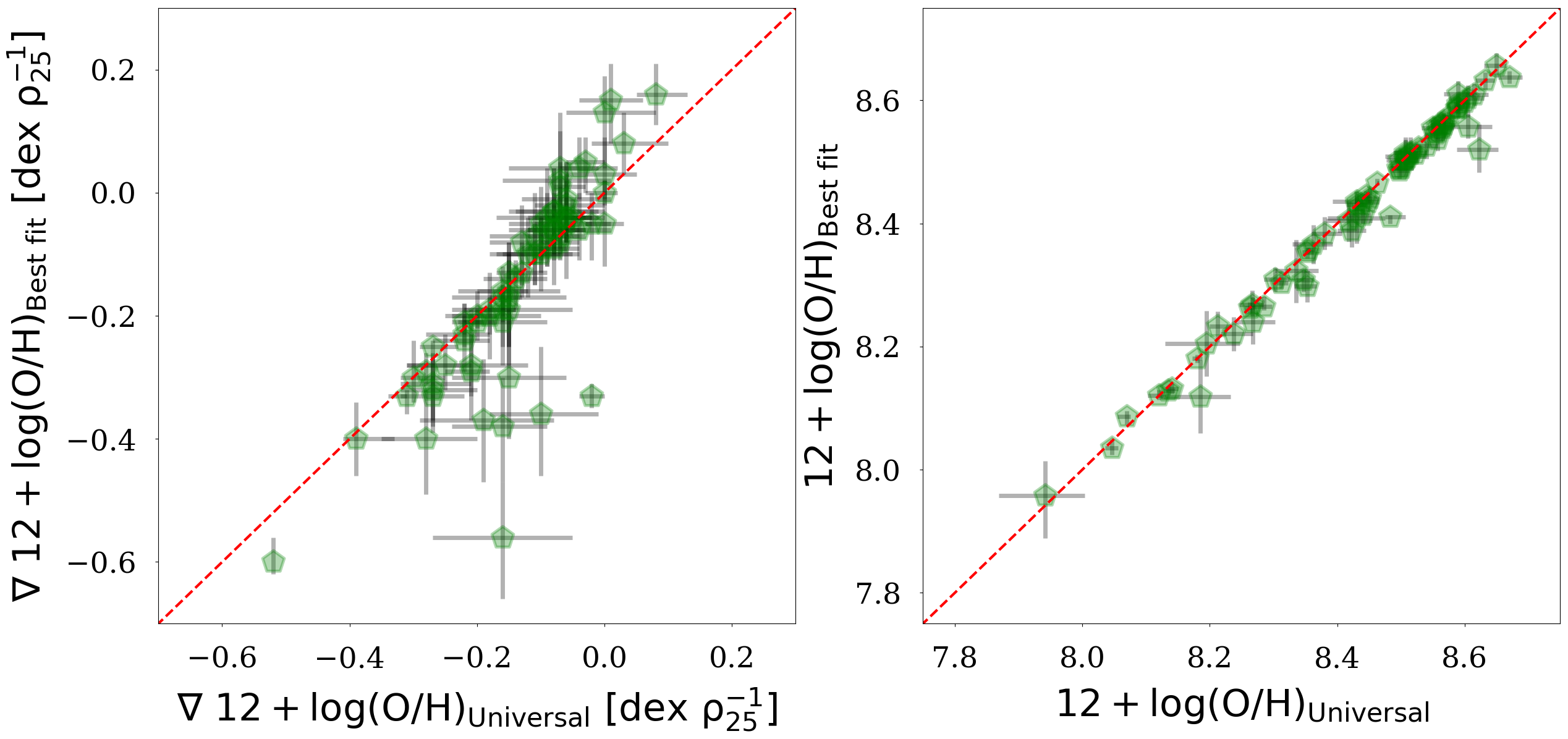
We compare our global metallicities estimated from IFU and fibre metallicities to measured global metallicities for the 110 sources which have both estimates available. The resulting comparison is shown in Figure 4. There is a good match between the two estimates, indicating that our method performs well. Finally, we also tested using the ‘universal prior’ for the gradients for all galaxies, rather than just for the unconstrained sub-sample. When the results are compared, we find the effect on the global metallicities is negligible, though there are some significant offsets on the resulting gradients, where the ‘universal prior’ results are biased towards the mean of the sample99 9 When the ‘universal prior’ is used, the comparison with other samples is less good (Section 6.1).. Therefore, we consider our global metallicities to be reliable, even for the unconstrained sub-sample. However, the measured gradients for the unconstrained sub-sample are likely to be unreliable and we used them no further.
4 Other galaxy properties
4.1 DustPedia
Dust masses, stellar masses and star formation rates (SFR) for the DustPedia galaxies will be presented in Nersesian et al. (in prep.). These results are derived from the aperture-matched DustPedia Photometry presented in Clark et al. 2018 using the SED fitting package CIGALE (Noll et al. 2009). CIGALE creates a library of SED templates for which the energy balance between the energy absorbed by dust in the UV-optical and the energy re-emitted in the infrared is maintained. This library is build assuming a delayed and truncated SF history (Ciesla et al. 2016) along with stellar emission from the stellar population models of Bruzual & Charlot 2003 and a Salpeter initial mass function. For the dust emission, the THEMIS (Jones et al. 2017) dust grain model is used, which is the reference DustPedia dust model. Using Bayesian statistics the best values and uncertainties for the , and SFR are determined.
To obtain Hi masses for the DustPedia sample we have performed a literature compilation (see also Casasola et al. in prep.). Integrated Hi fluxes were found for 764 out of the 875 DustPedia galaxies. The various references used for this compilation are listed in Table 2. 569 sources were found with Hi-detections and listed uncertainties, 96 galaxies have Hi-detections but no listing for the uncertainty and 99 galaxies have upper limits available only. When multiple references were available, preference was given to the measurements with the smallest uncertainty. There are 67 ALFALFA sources for which the DustPedia aperture from Clark et al. 2018 is larger than and there might thus be some Hi flux outside the ALFALFA aperture. The Hi flux for these sources was therefore corrected to account for Hi outside of the ALFALFA aperture using the Hi-profile from Wang et al. 2014, who found the Hi discs of galaxies exhibit a homogeneous radial distribution in their outer regions, and provide scaling relations between the scale length and .
This method of correcting the ALFALFA Hi flux seemed to give more reliable results than using alternative observations or methods available in the literature (which often differed by a factor of 1.5 or more). We note that the upper limits are not calculated consistently between all the different references. The most realistic upper limit should be given by , where and are the rms (in Jy) and width (in km/s) for a given channel, and is the estimated width of the Hi-line. Some of the references in our compilation do not take into account the channel width. We have not used upper limits in this work, but include them (as published) in our compilation for completion. Hi fluxes were converted to using:
| (6) |
where is the compiled Hi flux in Jy km s-1 and is the best distance measure from Clark et al. 2018 in Mpc. To obtain gas masses, we first added to the Hi. We refer the reader to Casasola et al. (in prep.) for a study of the content of DustPedia galaxies. Unfortunately, we do not have global masses available for all our galaxies, so instead we use a scaling relation between the -to-Hi ratio and the Hi-to-stellar mass ratio to estimate global masses. Casasola et al. (in prep.) find the following relation.
| (7) |
The gas mass is then determined as
| (8) |
where is taken from Casasola et al. (in prep.) when detections are available and estimated using Eq. 7 if not. is a correction factor to account for the fraction of the gas that is made up of elements heavier than hydrogen. We follow Clark et al. 2016 and define as
| (9) |
where is the primordial Helium mass fraction of 0.2485 (Aver et al. 2011), is the fraction of metals by mass and (Balser 2006) is the evolution of the helium mass fraction with metallicity. The correction factor varies from for zero metallicity to for solar metallicity. The measurement uncertainties on and the uncertainties on the estimated (about 0.5 dex) are propagated into the uncertainty on . This uncertainty on often dominates the total uncertainty.
In this work, we followed 60 in using gas fraction () as a rough proxy for evolutionary stage. Due to inflows and outflows of gas, there is not necessarily a monotonic relation between the gas fraction and the evolutionary stage of a galaxy. Even so, gas fraction remains a good tracer of the evolutionary stage as it is a measure of how much future star formation can currently be sustained, relative to the past star formation.
4.2 Comparative samples
| Name | SFH | Reduced SN dust | Destruction | Grain growth | Inflow | Outflow |
|---|---|---|---|---|---|---|
| Model I | Milky Way | N | N | N | N | N |
| Model V | Delayed | SFR | SFR | |||
| Model VI | Delayed/3 | SFR | SFR |
Due to its 5 detection in the WISE W1 band and diameter () selection criteria, DustPedia is somewhat biased against dwarf galaxies. Yet it is exactly these dwarf galaxies that have the lowest metallicities, which makes them a key stage to observe the evolution in the dust-to-metal ratios. Therefore, we increase our statistics at the low-metallicity end by adding the Dwarf Galaxy Survey (DGS; Madden et al. 2013 Madden et al. 2013), the dust-selected HAPLESS (Clark et al. 2015) and Hi-selected HiGH (De Vis et al. 2017a) sample to our study. Only sources that are not in the DustPedia sample are added. Galaxy properties for each of these samples were compiled in 60. We used their metallicities, SFR, stellar masses, and Hi masses as published, though their dust masses were derived with MAGPHYS (da Cunha et al. 2008) rather than CIGALE, and thus do not use the THEMIS dust model. MAGPHYS uses a dust mass absorption coefficient of , and the THEMIS dust mass absorption coefficient is well described by for in (Galliano et al. 2018). We therefore scaled the 60 dust masses down by a factor of 1.075. Total gas masses for these samples were calculated using the 60 Hi masses and Equation 8.
In addition, we compared our observations to some of the chemical evolution models presented in 60. In summary, these models track the global gas, stellar, metal, and dust content of a galaxy as gas is converted into stars (using a Chabrier IMF) as a result of a given star formation history. Dust and metals are expelled into the ISM when stars reach the end of their life at an age appropriate for their mass. The models separately track the oxygen (used for ) and total metal content (total mass of metals). The models also include prescriptions for inflows and outflows (proportional to the SFR), dust destruction and dust grain growth. The dust mass evolution is described by
| (10) |
The first term accounts for dust formed in stars and supernovae. The second term describes the removal of dust due to astration (destruction of dust mixed with the gas that is consumed during star formation) and the dust destruction and grain growth are given in terms three and four. The fifth and sixth term are simple parameterisations of dust contributed or removed via inflows and outflows. In more detail, the stellar term integrates over all stellar masses using a Chabrier IMF, the lifetimes of the stars at each mass, and LIMS and SN dust yields for each mass. The dust destruction term is due to SN-driven shocks and is described by
| (11) |
Here gives the fraction of the dust that is in the dense phase, which we have set to 50%. The timescale for dust destruction (, following Dwek et al. 2007) is described as a function of the rate of SN ():
| (12) |
where is the mass of ISM that is swept up by each individual SN event. The following prescription is used for the dust grain growth:
| (13) |
The dust grain growth timescale uses the prescription of Mattsson & Andersen 2012 and is given by
| (14) |
where Z is the fraction of heavy elements, is the mass of metals, and is a dimensionless free parameter which is varied to set the appropriate rate of dust grain growth. The inflows and outflows of gas are simple parametrisations proportional to the SFR. The inflows in this work are pristine gas and the inflow term in Equation 10 thus becomes zero. The outflows drive out dust at a rate which is the product of the current dust-to-gas ratio and the gas outflow rate. In this work we compare the DustPedia observations to three models from 60. The parameters used for these three models are given in Table 2. The aim here is not to find the best model or to constrain the dust evolution parameters, but rather to put our DustPedia observations into context and to provide a basic interpretation for the observed trends. The DustPedia data will be used in future work to constrain a next generation of chemical evolution models.
Model I is the simplest model, with only stellar source of dust and no inflows or outflows. It uses a Milky Way-type exponentially declining SFH. The dust yield per SN is mass and metallicity dependent and is taken from Todini & Ferrara 2001. This is not the most realistic model, but is included here to illustrate the failures of such a simple model. Models V and VI are more realistic and include prescriptions for dust grain growth, dust destruction, delayed SFH and inflows and outflows. Both Model V and VI have outflows with constant mass loading factors (outflow SFR) and inflows at the same rate as the outflows. Model V has stronger dust destruction (; Dwek et al. 2007), consistent with dust destruction in the diffuse ISM. For Model VI , indicative of SN shocks ploughing into typical interstellar densities of (Gall et al. 2011; Dwek & Cherchneff 2011). Additionally, Model VI has faster grain growth (higher ) than Model V. Finally, the Todini & Ferrara 2001 dust yield per SN is also reduced in both models. This reduction in dust yield is likely necessary to account for the reverse shock in the remnants of SN (Bocchio et al. 2016, e.g.). For Model V the dust yield is reduced less than for Model VI. We note that there is a degeneracy between the dust destruction (Eqn. 12 and reduced dust yield) and dust grain growth, and as a result both Model V and VI provide reasonably well fitted models (though further work on improving the models is underway).
5 Results
5.1 Radial gradients


| Calibration | ||
|---|---|---|
| PG16S | -0.15 | 0.16 |
| PG16R | -0.20 | 0.21 |
| N2 | -0.09 | 0.21 |
| O3N2 | -0.16 | 0.25 |
| IZI | -0.17 | 0.26 |
| KK04 | -0.24 | 0.25 |
| T04 | -0.18 | 0.29 |
| -0.38 | 0.34 |
Before studying the global DustPedia metallicities, we investigated in this section whether the gradients within our well-sampled galaxies correlate with any other galaxy properties. The average gradients and standard deviations for each calibration are given in Table 3. There are significant differences between the different calibrations (see Section 6.1). In Figure 5 (left), we have plotted how the gradients depend on stellar mass for all the sources in the well constrained sub-sample (at least five data points covering a range of radii at least wide). No significant correlation is found (Spearman’s rank correlation coefficient ). This is consistent with the findings of Sánchez et al. 2012a; Sánchez et al. 2014; Ho et al. 2015; Sánchez-Menguiano et al. 2016. However, we refer the reader to Section 6.1 where we show that this result depends on the calibration used.
When the parameter-space is further explored, we find a number of galaxy properties which yield a stronger (though still relatively weak) correlation with the metallicity gradient than stellar mass. When the gradient is plotted against , Spearman’s rank correlation coefficient increases to . With respect to the dust properties, the strongest correlation with the metallicity gradient is found with (Spearman ). We also plot the gradient against the effective radius (Spearman ) from Sérsic (Sérsic 1963; Sérsic 1968) fits1010 10 These Sérsic fits are based on WISE 3.4 m imagery (i.e. they trace the old stellar population). from Mosenkov et al. 2018, we find that galaxies with the largest physical extent, have the strongest gradients1111 11 Using the effective radius instead of in the calculation of the gradients (i.e. using instead of ) yields a correlation that is not very different.. Tortora et al. 2010 have found a similar correlation between the optical colour gradients and in a sample of 50000 nearby SDSS galaxies. The metallicity gradients and colour gradients are likely an effect of the same mechanism. Hydrodynamical simulations suggest galaxies with a larger extent have larger rotational velocities relative to the velocity dispersion. This could result in less mixing of the gas and dust at different radii and thus steeper gradients.
5.2 DustPedia oxygen abundances
To highlight the differences between the various calibrations used in this work, we plot the M-Z relation for each calibration in Figure 6. We plot the global DustPedia metallicities using PG16S (our reference calibration; see section 3.2), and add the HiGH, HAPLESS and DGS samples to obtain better statistics at the low-metallicity end. We also have global metallicities available for each of the different calibrations (not plotted as this would overcrowd the plot), and have fitted a third order polynomial to the metallicities for each of the different calibrations (plotted in dashed lines). The best-fitting third order polynomials are similar in shape, though have a different y-axis intercept. This discrepancy towards higher metallicities for theoretical calibrations (based on photo-ionisation models) is well known in the literature (Kewley & Ellison 2008; Moustakas et al. 2010, e.g. ). We provide metallicity calibration conversions between PG16S and the other calibrations in this work in Appendix B.

Next we show how the metallicity increases as galaxies evolve1212 12 Gas fraction is used as a proxy for evolution as it is a good measure of how much star formation can be sustained from the current gas reservoir, compared to the star formation that has already happened. Though inflows and outflows of gas and mergers will also affect the gas fraction. in Figure 7. The metallicity is found to increase monotonically with decreasing gas fraction. When the data are compared to chemical evolution models, we find that significant inflows and outflows are necessary to avoid significantly overestimating the model metallicity at low gas fractions (Models V and VI; 60). Using our larger DustPedia sample, it now becomes clear that Models V and VI still overestimate the metallicity for the earlier stages of evolution (gas fraction ). This is likely because for these models, the strength of the inflows and outflows shows the same proportionality with SFR for all galaxies, whereas in reality low mass galaxies (which have higher gas fractions) will be affected by outflows more strongly than high mass galaxies because they have a weaker gravitational potential to counteract the outflows. The remaining mismatches between models and observations might be alleviated by including models with higher mass loading factors for low mass galaxies, which would decrease the model metallicity at early evolutionary stages. We are working on a new set of chemical evolution models which will include this dependency (De Vis et al. in prep.).

In Figure 8, we show how the nitrogen to oxygen ratio (N/O) evolves with gas fraction. There is a significant correlation (Spearman’s rank correlation coefficient ). Here only DustPedia galaxies are shown as 60 did not compile N/O ratios. The N/O is found to be more or less steady around until a gas fraction of 0.5 and then increases towards lower gas fractions. We attribute this to the fact that for high gas fractions, only primary N and O are available, yet for higher metallicities secondary (i.e. the yield depends on the previous amount of carbon and oxygen in the stars) N and O become available (Pérez-Montero et al. 2013). The increasing N/O can be explained by the faster production rate of secondary N than for O (Henry et al. 2000; Thuan et al. 2010). We note that many galaxies in this plot have no uncertainties available. Many of these estimates come from references which present integrated spectroscopy without uncertainties. The lack of resolved data is due to the lack of [OII] emission line measurements (e.g. MUSE only provides spectra down to ) necessary for our N/O determination.

5.3 Evolution in the dust-to-metal ratio
In this section, the dust and metal content are compared to better understand the processes driving the dust evolution. We start by plotting the dust-to-gas ratio against (which by definition is a measure of the metal-to-gas ratio) for the 466 DustPedia galaxies which have all three of these measures available. In Figure 9, we find an increasing dust-to-gas ratio with increasing metallicity. The dust-to-gas ratio increases more steeply than Model I of the chemical evolution models. Model I only includes stellar sources of dust, and thus has a constant dust-to-metal ratio. The only way to obtain a steep enough increase of the dust-to-gas ratio, is to include dust grain growth in the models (Model V and VI). When Rémy-Ruyer et al. 2014 studied this relationship, they found a broken power law provides a good empirical fit to the data. We find this relation results in slightly higher dust-to-gas ratios than the average for our sample. Some of this offset might be due to the use of a different metallicity calibration1313 13 The Pilyugin & Thuan 2005 metallicity calibration used in this work cannot be reliably scaled into the different calibration methods used in this work (Kewley & Ellison 2008).. The Rémy-Ruyer et al. 2014 trend traces the DGS data at low metallicity, yet the observed DustPedia dust-to-gas ratios are lower in general. Our more complete sample of DustPedia galaxies is thus key to properly constrain models of the dust and chemical evolution of galaxies.
We have fitted a power law and broken power law to the DustPedia1414 14 We have not included the DGS, HIGH and HAPLESS samples in our fit to avoid any potential bias from the different selection criteria or methods used. LTGs for each of the metallicity calibrations using orthogonal distance regression (taking into account uncertainties on both the dust-to-gas ratios and metallicities). ETGs have not been included as dust destruction by hot gas sputtering might lower their dust-to-gas ratio (see also Figure 14 in Section 6.2). The results for single power laws are listed in Table 4. Contrary to Rémy-Ruyer et al. 2014, we find broken power laws do not provide a better description to the data as a single power law. When we followed Rémy-Ruyer et al. 2014 in fixing the slope for high metallicities to one (James et al. 2002; Galliano et al. 2008, see also e.g.), the fits to the data are formally worse than the single power law for all calibrations except N2 and K04. If this slope is left free, the fits are only marginally better than the single power law (in spite of two additional free parameters), and the slope for high metallicities is consistent within the errors with the single power laws listed in Table 4. The single power laws thus provide the best description of the dust build up with increasing metallicity. For each of the calibrations, the relation is super-linear, indicating that stellar dust sources alone (which would result in a slope of one) cannot explain these relations.
| calib. | ||||
|---|---|---|---|---|
| PG16S | 1.94 | 0.11 | -19.04 | 0.91 |
| PG16R | 1.83 | 0.15 | -18.13 | 1.22 |
| N2 | 1.62 | 0.10 | -16.71 | 0.85 |
| O3N2 | 1.77 | 0.10 | -17.96 | 0.86 |
| IZI | 1.45 | 0.10 | -15.30 | 0.82 |
| KK04 | 1.22 | 0.14 | -13.50 | 1.26 |
| T04 | 1.50 | 0.10 | -16.01 | 0.84 |
60 found a steep initial increase of the dust-to-gas ratio, followed by a more gradual increase (with constant dust-to-metal ratio). Using our larger DustPedia sample, there is no such clear break between these two regimes. The steep increase in these previous works could be explained by galaxies reaching the critical metallicity at which dust grain growth becomes effective. This steep increase is also seen in Models V and VI (at slightly different critical metallicities). However, in reality, the metallicity in a galaxy is not uniform (as is assumed in these models). The critical metallicity will be reached at different points in time for different regions in the galaxy (inside-out evolution, which also results in the observed metallicity gradients), and as a result the increase in the dust-to-gas ratio will be more gradual. Further resolved chemical evolution modelling (Aoyama et al. 2016; McKinnon et al. 2016; McKinnon et al. 2018, such as) is necessary to study this behaviour in detail.

In what follows, we have studied the evolution of the dust-to-metal ratio with other galaxy properties. The mass of metals is calculated as where is the fraction of metals by mass calculated using . The factor of 27.36 is found from assuming and a Solar metal mass fraction following Asplund et al. 2009. Throughout this work we track the total mass of metals in the ISM (i.e. including metals locked up in dust).
In reality, the fraction of oxygen to the total mass of metals will not be constant throughout the evolution (see e.g. varying N/O in previous section). From studying the 60 chemical evolution models where the mass of oxygen and total mass of metals are tracked separately, we find that these differences are of the order of (0.1 dex). It should be kept in mind that in what follows, we are essentially tracking changes in the dust-to-oxygen mass ratio (re-scaled to dust-to-metal ratio using a fixed oxygen-to-metal ratio) rather than in the intrinsic dust-to-metal mass ratio.
Plotting the dust-to-metal ratio against metallicity and gas fraction (both tracers of the evolutionary stage) in Figure 10, a significantly lower is found for the earliest stages of evolution. This behaviour is also followed by Models V and VI (see Section 6 for further discussion), where for some galaxies Model V provides the best fit, yet for others Model VI is better. The overall correlations are quite weak (Spearman and for metallicity and gas fraction respectively). We find that DustPedia galaxies with gas fractions below (or above ) have a more or less constant dust-to-metal ratio of . For the other calibrations in this work the dust-to-metal ratio is also constant over the same range of gas fraction (or metallicity), though due to the discrepancy towards higher metallicities, the dust-to-metal ratio is lower for the other calibrations. Table 5 shows the average for evolved galaxies for each calibration.
| calib. | ) | ||
|---|---|---|---|
| PG16S | 0.214 | -0.67 | 0.21 |
| PG16R | 0.206 | -0.69 | 0.21 |
| N2 | 0.162 | -0.79 | 0.23 |
| O3N2 | 0.151 | -0.82 | 0.23 |
| IZI | 0.141 | -0.85 | 0.26 |
| KK04 | 0.116 | -0.93 | 0.30 |
| T04 | 0.092 | -1.04 | 0.25 |
For gas fractions greater than and metallicities below , the average dust-to-metal ratio starts to differ significantly. DustPedia galaxies with gas fractions greater than have an average , and galaxies with gas fractions greater than have an average . However, even at these early evolutionary stages, some galaxies still have high , and the scatter in is thus quite high (standard deviation of dex). Part of this scatter can be attributed to the increased uncertainties as a result of these galaxies being fainter. We do indeed see larger error bars for the unevolved galaxies in Figure 10. Yet even for the well constrained sources, the scatter remains large. The remaining differences in at these evolutionary stages can be explained by differences in the local conditions and SFH (see also Section 6.2). In particular, Schneider et al. 2016 have shown differences in the density of the cold ISM can result in large differences in the dust mass. Galaxies with high in spite of high gas fractions, probably have an unusually dense ISM and a corresponding fast dust grain growth timescale.


In Figure 11 we explore how the dust-to-metal ratio scales with other galaxy properties such as stellar mass and the specific SFR (sSFR). For low stellar masses, we find a very weak correlation (Spearman rank correlation coefficient ) and again find a lower dust-to-metal ratio and large scatter, as was expected since low stellar mass sources typically have high gas fractions. Sources with stellar masses larger than have a fairly constant dust-to-metal ratio of with a standard deviation of dex. This is slightly lower, yet consistent with the average value for low gas fraction () sources. When the dust-to-metal ratio is plotted against sSFR, we find a weak but significant correlation (Spearman ) over the whole range of sSFR, though with significant outliers. There are a number of DGS sources which have very high sSFR, in spite of having already gone through some evolution in the past (they have moderate gas fractions, metallicities and stellar masses). These galaxies are currently undergoing a starburst (60), which results in an increased sSFR that is not matched by an equivalent decrease in .


6 Discussion
6.1 Radial gradients
There are numerous studies that have looked at metallicity gradients. Some of the galaxies in these studies are also in our sample. For these common galaxies, we can thus compare our gradient estimates to validate our method. Figure 12 shows the common galaxies between our sample and the sample from Moustakas et al. 2010. We used the KK04 calibration for both sets of results. We find relatively consistent results, with only one strong outlier (NGC3621). The average , which drops to if the outlier is discarded. Our gradient for NGC3621 is likely different since we have data out to larger radii (though there is no evidence for a change in the gradient between the central and outer regions). Our gradient for NGC3621 is also more similar to the gradient for other calibrations (Moustakas et al. 2010 find a big difference between their KK04 and PT05 calibration for NGC3621).

There are significant differences between different metallicity calibrations and the resulting radial gradients (Section 5). Using KK04, Moustakas et al. 2010 find an average gradient of . This is significantly steeper than our average KK04 gradient in Table 3. However, if we only consider our sources in common with Moustakas et al. 2010, we find an average KK04 gradient of , which is consistent with Moustakas et al. 2010 within the uncertainties. The average O3N2 gradient from CALIFA is (Sánchez et al. 2014), consistent with our O3N2 results. The average O3N2 gradient of Ho et al. 2015 is , slightly steeper than our average, which is likely due to Ho et al. 2015 only selecting star-forming field galaxies.
In addition to different calibrations, some works in the literature (Belfiore et al. 2017; Poetrodjojo et al. 2018, e.g.) normalise the radii by instead of . Therefore, caution is necessary when comparing our results to the results in the literature. In contrast with our results in Section 5.1 for PG16S, Belfiore et al. 2017 and Poetrodjojo et al. 2018 find a weak but significant trend between the metallicity gradient and stellar mass. To compare consistently, in Figure 13 we plot the relation between metallicity gradient and stellar mass using the O3N2 and KK04 calibrations instead of PG16S. In addition, we normalise our radii by instead of for consistency. We find very weak correlations (Spearman and for O3N2 and KK04 respectively), though now our results are more similar to the results from Belfiore et al. 2017 and Poetrodjojo et al. 2018. The binned results from Belfiore et al. 2017 do indeed look sensible when compared to our data and the difference could simply be due to the limited size of our sample with well constrained gradients. These differences show that the choice of calibration and normalisation of the radii can cause important differences in the results.


Hydrodynamical simulations suggest that the underlying process that is responsible for the average negative metallicity profiles is the inside-out formation of discs with specific angular momentum conservation (Tissera et al. 2016). However, dynamical processes such as mergers perturb the metallicity distributions, and typically result in flatter or even positive gradients. However, if this merger is followed by a central starburst, the newly produced heavy elements steepen the gradients again, yet they often remain above the values (i.e. flatter) that would otherwise be expected (Tissera et al. 2016; Perez et al. 2011). In addition, outflows of enriched material from the central regions could be re-accreted at larger radii, and thus contribute to flattening the metallicity profiles (Perez et al. 2011). The common slope for PG16S can be explained if all disk galaxies went through very similar chemical evolution when building up their disks.
Even though our metallicity determinations have been performed consistently across our whole compilation, the sampling of regions in different galaxies is quite heterogeneous. Some galaxies have very well sampled IFU data, whereas others have a few or even only one fibre spectrum. Therefore, we assessed whether our gradient determination is biased towards a particular parameter-space. We studied the dependency of the gradients on any of the following parameters:
- •
The number of data points we have available for a specific galaxy.
- •
The radial distance to the most distant available data point.
- •
The total radial distance covered by our data points.
- •
The selection bias of IFU data towards high metallicity galaxies.
- •
The number density of the local environment (from Davies et al. in prep.).
We find no dependence of the average gradient, nor the scatter, on any of these parameters. We note that we are only considering the well constrained sub-sample and galaxies with very few data points have thus been discarded (these would be biased towards the mean gradient and show less scatter). There is a small interdependency between the number of data points (selection bias of IFU data) and other galaxy properties such as stellar mass and SFR (massive actively star-forming galaxies often have more metallicity data points available on average), though this does not carry through to any bias in the metallicity gradients.
6.2 Dust-to-metal ratio
Our sample is the largest sample of galaxies for which the dust and metal content are measured consistently over all galaxies. When we combine DustPedia with the 73 galaxies in our comparison samples, we arrive at a sample of 539 sources (compared to 382 for the combined sample in 60). In addition to the better statistics and better consistency across samples, our sample has made use of the resolved information in these galaxies to arrive at a better estimate of the global estimate. Our data has revealed a more gradually and continuously evolving dust-to-metal ratio, rather than two separate regimes for high and low metallicity galaxies (as in Rémy-Ruyer et al. 2014, and DV17). The more gradual increase is attributed to different regions in the galaxy reaching the critical metallicity at different times.
In the literature, the dust-to-metal ratio of galaxies is often assumed to have a constant value of around (e.g. James et al. 2002 James et al. 2002; Clark et al. 2016 Clark et al. 2016; Camps et al. 2016 Camps et al. 2016). This is slightly higher than what we find for evolved DustPedia galaxies (), though for unevolved galaxies significantly lower values are found. We note that our estimate of the dust-to-metal ratio should not be used at face value for high redshift galaxies. At high redshifts, high stellar mass galaxies are still in early evolutionary stages (and have high gas fraction and low metallicity), and thus likely have low dust-to-metal ratios.
A consistent picture emerges from our results in the previous sections: Galaxies start out with low dust-to-metal ratios, which then increase as galaxies evolve, and finally remain constant in the later evolutionary stages. Dust grain growth provides the most likely explanation for this behaviour. For unevolved galaxies the metallicities are very low and conversely their dust grain growth timescales are very long (Eq. 14). As the metal content increases, the efficiency of the grain growth increases as there are more and more metals available to accrete onto the dust grains. For DustPedia galaxies the critical metallicity is around , consistent with other work (Galliano et al. 2018). The increase in the dust-to-metal ratios levels off towards high metallicities or low gas fractions as most of the available metals are depleted onto the dust grains. At the same time global dust destruction (Eq. 12; i.e. not the reverse shock in SN) processes reduce the dust-to-metal ratio. The observed increase shows these destruction processes are not dominant, yet they do contribute to some extent. At the start of the evolution, the dust-to-metal ratio is set by a balance between dust destruction and dust production by stars, yet later it is set by a balance between dust destruction and dust grain growth (Mattsson et al. 2014).
Our chemical evolution model without dust grain growth (Model I) clearly fails to explain the observations. Variations of Model I (e.g. including inflows and outflows, different SFH.) also cannot obtain a good match to the observations unless dust grain growth is included and the SN dust yield is reduced. Models V & VI do include dust grain growth and reduced SN dust and consequently provide a good match to our data. We note that the scatter in our observations at high gas fractions is large, and as a result the observations cannot be described by a single model. In De Vis et al. (in prep.) we will explore a grid of models where each of the free parameters will be varied. In particular we expect the following parameters to cause significant variations between the different galaxies at a fixed gas fraction.
The first important parameter is the SFH. Galaxies typically go through one or more burst of star formation throughout their evolution. The start time and duration of these burst can (temporarily) affect the dust-to-metal ratio (Zhukovska 2014, e.g.). During the burst, a lot of metals are expelled, which have not yet had time to accrete onto the grains, and decreases. After the burst, dust grain growth continues until all the newly available metals are accreted. Variations in the grain growth timescale will also strongly affect the dust-to-metal ratio. Local conditions (such as ISM density; Schneider et al. 2016 Schneider et al. 2016) could significantly influence the dust grain growth timescales. Very fast ( Myr) timescales conform with Feldmann 2015 result in high , even for unevolved galaxies. Additionally, variations in the strength of the reverse shocks could result in scatter in the SNe dust yields and thus scatter in .
Each of these three parameters could easily be affected by the individual conditions within a galaxy. A galaxy merger could, for example, result in a burst of star formation, as well as change the density of the ISM, which could in turn result in different grain growth timescales, and a different strength of the reverse SN shock. Additionally, uncertainty remains over the dust and metal yield of SN and AGB stars. AGB dust yields could be metallicity dependent (Ferrarotti & Gail 2006, e.g.), and more recent SN dust yield prescriptions (Bianchi & Schneider 2007; Marassi et al. 2018) could be used. However, Ginolfi et al. 2018 show that, independent of the adopted (metallicity-dependent) AGB and SN dust yields, models without grain growth cannot explain the observed trends.
Instead of dust grain growth as the driver of the evolution, varying the SN dust yields could provide an alternative explanation. If the SN condensation efficiency (dust yield per metal yield) increases as galaxies evolve, there is no need for dust grain growth. However, the SN condensation efficiency is not expected to vary by more than a factor of three (Dwek 1998; Todini & Ferrara 2001) and cannot explain the observed variation of an order of magnitude. However, these yields do not take into account the reverse shock. One option is that dust destruction by the reverse shock is much stronger in unevolved galaxies than at later evolutionary stages. Dust destruction by the reverse shock is expected to be stronger if the local ISM density around the SN is significantly higher in unevolved galaxies (Bianchi & Schneider 2007; Bocchio et al. 2016). There is little information in the literature about how the strength of the reverse shock and the local ISM density change in various environments, so we cannot discount this possibility. However, we note that without any dust grain growth, SN would have to produce more than five solar masses of dust to explain the galaxies with the highest . This is inconsistent with the dust content of SN remnants (which have not yet been processed by the reverse shock).
Another important point to discuss is how the selection of our sample affects the relations found. In particular, by including only sources with detected metallicities, we have excluded a part of the parameter-space. In Figure 14, we show the dust-to-gas ratio against gas fraction for the metal-detected sources used in this work, together with all DustPedia sources for which we have a detected Hi mass (i.e. including the ones without metallicities). For the Hi-detected sources, there is a population of low gas fraction ETGs with dust-to-gas ratios that are significantly lower (by more than an order of magnitude) than the rest of the sample. Presumably, sputtering by hot gas has destroyed a lot of the dust in these galaxies. When we focussed on the metal-detected sources, however, we find that this population of sources has entirely been missed. Upon inspection we find that these galaxies only have AGN-classified optical spectra available. If we assign these sources a metallicity that is typical for their gas fraction, they have significantly lower dust-to-metal ratios than the rest of the sample.

Finally, we would like to note two potential caveats to our method. The first is that we assumed, as in almost all studies concerning dust, that the dust mass absorption coefficient is constant. However, our changes in dust-to-metal ratio could also be interpreted as changes in the dust mass absorption coefficient at a constant dust-to-metal ratio. This alternative interpretation has actually been used to constrain for evolved galaxies (James et al. 2002; Clark et al. 2016). Our second caveat is that we used the total gas mass from single dish observations, whereas some of the Hi might actually be extended beyond our aperture from Clark et al. 2018. This Hi gas might be extra-planar gas that is not actually associated with the galaxy (Vargas et al. 2017, e.g.), and thus not affecting the dust properties. An overestimation of the galaxy gas mass would also lead to an overestimation of the metal mass and thus to lower dust-to-metal ratios. Dwarf galaxies (which typically have higher gas fractions) could be more strongly affected by this issue, thereby introducing a bias in our results. Roychowdhury et al. (in prep.) are investigating DustPedia dwarf galaxies using resolved Hi data to study this issue in more detail.
7 Data products
This work presents a large, homogeneous set of resolved and global metallicity measurements of 516 nearby galaxies (10143 individual regions). In combination with the available multi-wavelength imagery and photometry (Clark et al. 2018), as well as galaxy properties from SED fitting (Nersesian et al. in prep.) and the Hi measurements, this forms an unprecedented database which will be invaluable for future investigations of galaxy (chemical) evolution processes. The data in this work is available as four separate tables, which can be accessed on the DustPedia archive1515 15 http://dustpedia.astro.noa.gr/AncillaryData, and from the VizieR catalogue service1616 16 Will be uploaded after publication of the of the paper. The references used for our compilation and examples of each of the four tables are given in Appendix C. The first table list the Hi fluxes, uncertainties, and masses (Section 4.1). The next table lists the reddening-corrected emission line fluxes for the compiled emission lines from the literature, combined with the extracted MUSE spectrophotometry (see Section 2), for all the regions that are classified as star-forming. The third table lists the oxygen abundances and corresponding bootstrapped uncertainties using multiple calibration methods for each of these star-forming regions. The reddening coefficients are listed in both the emission line and metallicity table for each individual region (for MUSE both reddening components have been added). Our final table presents the available global metallicities for each of the galaxies in our sample, together with their uncertainties as detailed in Section 3.4.
8 Conclusions
We have studied the relative dust, gas, and metal content of DustPedia galaxies. By performing a literature search, combined with archival MUSE data, we were able to compile metallicities for 10143 individual regions within DustPedia galaxies. Radial profiles were fitted to these regions and global metallicities determined for 516 DustPedia galaxies by taking the metallicity at a radius of . All the metallicity measurements are made available to the community. A total of 466 DustPedia galaxies have all the necessary observations to constrain dust, gas and metal content. 76 of these have metallicities below (22 sources below ), providing key constraints on the evolution of the dust-to-metal ratios in early evolutionary stages. The DustPedia observations were also compared to additional samples, as well as simple chemical evolution models from De Vis et al. 2017b. Our main conclusions are:
- •
The gradient from a linear fit to the radial metallicity profile shows no significant dependence on stellar mass. Yet, the gradient was found to correlate weakly with the Hi-to-stellar ratio, the extent of the galaxy and with the dust-to-stellar mass ratio. The metallicity gradients depend on which calibration is used and whether the radii are normalised by or .
- •
The oxygen abundance is found to increase monotonically as galaxies evolve from high to low gas fractions. Chemical evolution models including inflows and outflows are necessary to explain the results. The nitrogen-to-oxygen ratio () is also found to increase monotonically with decreasing gas fraction, though it shows more scatter.
- •
The relation between the dust-to-gas ratio and metallicity is best described by a single powerlaw (), rather than a broken power law.
- •
For more evolved galaxies, we find a more or less constant dust-to-metal ratio. For galaxies with gas fraction below , metallicities above or stellar masses above , the dust-to-metal ratio is about .
- •
At early evolutionary stages (gas fraction above , metallicities below ), the average DustPedia galaxy has 2.1 times lower dust-to-gas and dust-to-metal ratios (6 times lower for galaxies with gas fraction ). However, at these early evolutionary stages there is quite a lot of scatter. Some galaxies have dust-to-metal ratios as high as evolved galaxies (), yet other galaxies have dust-to-metal ratio as low as . This increased scatter is likely to be due to variations in the local conditions and SFH resulting in different dust grain growth timescales and SN dust yields, combined with increased uncertainties due to these galaxies being fainter.
- •
We also find a decrease in the dust-to-metal ratio for low stellar masses and high sSFR. Though the larger scatter indicates these are likely indirect correlations. Bursty sources such as some of the DGS galaxies, have high sSFR yet have a high dust-to-metal ratio that is consistent with their gas content rather than with their star formation activity.
- •
By including only sources with detected metallicities (spectra classified as star-forming), we have missed a population of low gas fraction, low dust-to-gas ratio ETGs. These sources presumably have lower dust-to-metal ratios than the rest of the sample. Most likely, sputtering by hot gas has destroyed a lot of dust in these galaxies.
- •
We have compared these results to simple chemical evolution models. We find models with a dominant contribution to the dust budget from grain growth do a decent job at describing the observations. Resolved chemical evolution models would result in a less steep increase in the dust-to-metal ratio (thereby providing a better match to the observations), as well as allowing the study of metallicity and dust-to-metal gradients, which is the logical next step.
Acknowledgements.
DustPedia is a collaborative focused research project supported by the European Union under the Seventh Framework Programme (2007-2013) call (proposal no. 606847). The participating institutions are: Cardiff University, UK; National Observatory of Athens, Greece; Ghent University, Belgium; Université Paris Sud, France; National Institute for Astrophysics, Italy and CEA, France. We thank the referee, Raffaella Schneider, for helpful comments. We gratefully acknowledge Sebastian Sanchez and Laura Sanchez-Menguiano for their help with the CALIFA data. We also thank Leonid Pilyugin for sharing the data from Pilyugin et al. 2014 and useful comments. This work is based on publicly available MUSE data obtained from the ESO Science Archive Facility under request number pdevis291121. This research made use of the NASA/IPAC Extragalactic Database (NED), which is operated by the Jet Propulsion Laboratory, California Institute of Technology, under contract with the National Aeronautics and Space Administration. We acknowledge the usage of the HyperLeda database (Makarov et al. 2014 Makarov et al. 2014; http://leda.univlyon1.fr). This research made use of the VizieR catalogue access tool (Ochsenbein et al. 2000), CDS, Strasbourg, France.References
- Alam et al. (2015) Alam, S., Albareti, F. D., Allende Prieto, C., et al. 2015, ApJS, 219, 12
- Annibali et al. (2010) Annibali, F., Bressan, A., Rampazzo, R., et al. 2010, A&A, 519, A40
- Aoyama et al. (2016) Aoyama, S., Hou, K.-C., Shimizu, I., et al. 2016, ArXiv e-prints [arXiv:1609.07547]
- Asano et al. (2013) Asano, R. S., Takeuchi, T. T., Hirashita, H., & Inoue, A. K. 2013, Earth, Planets, and Space, 65, 213
- Asplund et al. (2009) Asplund, M., Grevesse, N., Sauval, A. J., & Scott, P. 2009, ARA&A, 47, 481
- Aver et al. (2011) Aver, E., Olive, K. A., & Skillman, E. D. 2011, J. Cosmology Astropart. Phys., 3, 043
- Bacon et al. (2010) Bacon, R., Accardo, M., Adjali, L., et al. 2010, in Proc. SPIE, Vol. 7735, Ground-based and Airborne Instrumentation for Astronomy III, 773508
- Baldwin et al. (1981) Baldwin, J. A., Phillips, M. M., & Terlevich, R. 1981, PASP, 93, 5
- Balser (2006) Balser, D. S. 2006, AJ, 132, 2326
- Battisti et al. (2016) Battisti, A. J., Calzetti, D., & Chary, R.-R. 2016, ApJ, 818, 13
- Belfiore et al. (2017) Belfiore, F., Maiolino, R., Tremonti, C., et al. 2017, MNRAS, 469, 151
- Berg et al. (2015) Berg, D. A., Skillman, E. D., Croxall, K. V., et al. 2015, ApJ, 806, 16
- Bettoni et al. (2003) Bettoni, D., Galletta, G., & García-Burillo, S. 2003, A&A, 405, 5
- Bevan et al. (2017) Bevan, A., Barlow, M. J., & Milisavljevic, D. 2017, MNRAS, 465, 4044
- Bianchi & Schneider (2007) Bianchi, S. & Schneider, R. 2007, MNRAS, 378, 973
- Blanc et al. (2015) Blanc, G. A., Kewley, L., Vogt, F. P. A., & Dopita, M. A. 2015, ApJ, 798, 99
- Bocchio et al. (2016) Bocchio, M., Marassi, S., Schneider, R., et al. 2016, A&A, 587, A157
- Boselli et al. (2014) Boselli, A., Cortese, L., & Boquien, M. 2014, A&A, 564, A65
- Boselli et al. (2013) Boselli, A., Hughes, T. M., Cortese, L., Gavazzi, G., & Buat, V. 2013, A&A, 550, A114
- Bottinelli et al. (1980) Bottinelli, L., Gouguenheim, L., & Paturel, G. 1980, A&AS, 40, 355
- Bottinelli et al. (1982) Bottinelli, L., Gouguenheim, L., & Paturel, G. 1982, A&AS, 47, 171
- Bouchard et al. (2003) Bouchard, A., Carignan, C., & Mashchenko, S. 2003, AJ, 126, 1295
- Bresolin et al. (2012) Bresolin, F., Kennicutt, R. C., & Ryan-Weber, E. 2012, ApJ, 750, 122
- Bresolin & Kennicutt (2002) Bresolin, F. & Kennicutt, Jr., R. C. 2002, ApJ, 572, 838
- Bresolin et al. (1999) Bresolin, F., Kennicutt, Jr., R. C., & Garnett, D. R. 1999, ApJ, 510, 104
- Bresolin et al. (2009) Bresolin, F., Ryan-Weber, E., Kennicutt, R. C., & Goddard, Q. 2009, ApJ, 695, 580
- Bresolin et al. (2005) Bresolin, F., Schaerer, D., González Delgado, R. M., & Stasińska, G. 2005, A&A, 441, 981
- Bruzual & Charlot (2003) Bruzual, G. & Charlot, S. 2003, MNRAS, 344, 1000
- Bureau et al. (1996) Bureau, M., Mould, J. R., & Staveley-Smith, L. 1996, ApJ, 463, 60
- Calura et al. (2014) Calura, F., Gilli, R., Vignali, C., et al. 2014, MNRAS, 438, 2765
- Calura et al. (2017) Calura, F., Pozzi, F., Cresci, G., et al. 2017, MNRAS, 465, 54
- Calzetti et al. (2000) Calzetti, D., Armus, L., Bohlin, R. C., et al. 2000, ApJ, 533, 682
- Calzetti et al. (1994) Calzetti, D., Kinney, A. L., & Storchi-Bergmann, T. 1994, ApJ, 429, 582
- Camps et al. (2016) Camps, P., Trayford, J. W., Baes, M., et al. 2016, MNRAS, 462, 1057
- Cappellari & Emsellem (2004) Cappellari, M. & Emsellem, E. 2004, PASP, 116, 138
- Cardelli et al. (1989) Cardelli, J. A., Clayton, G. C., & Mathis, J. S. 1989, ApJ, 345, 245
- Casasola et al. (2004) Casasola, V., Bettoni, D., & Galletta, G. 2004, A&A, 422, 941
- Chamaraux et al. (1999) Chamaraux, P., Masnou, J.-L., Kazés, I., et al. 1999, MNRAS, 307, 236
- Charlot & Fall (2000) Charlot, S. & Fall, S. M. 2000, ApJ, 539, 718
- Chiang et al. (2018) Chiang, I.-D., Sandstrom, K. M., Chastenet, J., et al. 2018, ApJ, 865, 117
- Cid Fernandes et al. (2010) Cid Fernandes, R., Stasińska, G., Schlickmann, M. S., et al. 2010, MNRAS, 403, 1036
- Ciesla et al. (2016) Ciesla, L., Boselli, A., Elbaz, D., et al. 2016, A&A, 585, A43
- Clark et al. (2015) Clark, C. J. R., Dunne, L., Gomez, H. L., et al. 2015, MNRAS, 452, 397
- Clark et al. (2016) Clark, C. J. R., Schofield, S. P., Gomez, H. L., & Davies, J. I. 2016, MNRAS[arXiv:1603.04860]
- Clark et al. (2018) Clark, C. J. R., Verstocken, S., Bianchi, S., et al. 2018, A&A, 609, A37
- Colless et al. (2001) Colless, M., Dalton, G., Maddox, S., et al. 2001, MNRAS, 328, 1039
- Courtois et al. (2009) Courtois, H. M., Tully, R. B., Fisher, J. R., et al. 2009, AJ, 138, 1938
- Croxall et al. (2015) Croxall, K. V., Pogge, R. W., Berg, D. A., Skillman, E. D., & Moustakas, J. 2015, ApJ, 808, 42
- Croxall et al. (2016) Croxall, K. V., Pogge, R. W., Berg, D. A., Skillman, E. D., & Moustakas, J. 2016, ApJ, 830, 4
- Croxall et al. (2009) Croxall, K. V., van Zee, L., Lee, H., et al. 2009, ApJ, 705, 723
- da Cunha et al. (2008) da Cunha, E., Charlot, S., & Elbaz, D. 2008, MNRAS, 388, 1595
- Dai & Kochanek (2009) Dai, X. & Kochanek, C. S. 2009, ApJ, 692, 677
- Davies et al. (2017) Davies, J. I., Baes, M., Bianchi, S., et al. 2017, PASP, 129, 044102
- Davoust & Contini (2004) Davoust, E. & Contini, T. 2004, A&A, 416, 515
- de Bennassuti et al. (2014) de Bennassuti, M., Schneider, R., Valiante, R., & Salvadori, S. 2014, MNRAS, 445, 3039
- De Cia et al. (2016) De Cia, A., Ledoux, C., Mattsson, L., et al. 2016, A&A, 596, A97
- De Cia et al. (2013) De Cia, A., Ledoux, C., Savaglio, S., Schady, P., & Vreeswijk, P. M. 2013, A&A, 560, A88
- De Looze et al. (2017) De Looze, I., Barlow, M. J., Swinyard, B. M., et al. 2017, MNRAS, 465, 3309
- De Vis et al. (2017a) De Vis, P., Dunne, L., Maddox, S., et al. 2017a, MNRAS, 464, 4680
- De Vis et al. (2017b) De Vis, P., Gomez, H. L., Schofield, S. P., et al. 2017b, MNRAS, 471, 1743
- Disney & Pottasch (1977) Disney, M. J. & Pottasch, S. R. 1977, A&A, 60, 43
- Draine (2003) Draine, B. T. 2003, ApJ, 598, 1017
- Draine et al. (2007) Draine, B. T., Dale, D. A., Bendo, G., et al. 2007, ApJ, 663, 866
- Driver et al. (2016) Driver, S. P., Wright, A. H., Andrews, S. K., et al. 2016, MNRAS, 455, 3911
- Dunne et al. (2003) Dunne, L., Eales, S., Ivison, R., Morgan, H., & Edmunds, M. 2003, Nature, 424, 285
- Dwek (1998) Dwek, E. 1998, in Astronomical Society of the Pacific Conference Series, Vol. 133, Science With The NGST, ed. E. P. Smith & A. Koratkar, 249
- Dwek & Cherchneff (2011) Dwek, E. & Cherchneff, I. 2011, ApJ, 727, 63
- Dwek et al. (2007) Dwek, E., Galliano, F., & Jones, A. P. 2007, ApJ, 662, 927
- Edmunds (2001) Edmunds, M. G. 2001, MNRAS, 328, 223
- Edmunds & Eales (1998) Edmunds, M. G. & Eales, S. A. 1998, MNRAS, 299, L29
- Falco et al. (1999) Falco, E. E., Kurtz, M. J., Geller, M. J., et al. 1999, PASP, 111, 438
- Feldmann (2015) Feldmann, R. 2015, MNRAS, 449, 3274
- Ferrarotti & Gail (2006) Ferrarotti, A. S. & Gail, H.-P. 2006, A&A, 447, 553
- Fisher et al. (2014) Fisher, D. B., Bolatto, A. D., Herrera-Camus, R., et al. 2014, Nature, 505, 186
- Fixsen et al. (1996) Fixsen, D. J., Cheng, E. S., Gales, J. M., et al. 1996, ApJ, 473, 576
- Franco & Cox (1986) Franco, J. & Cox, D. P. 1986, PASP, 98, 1076
- Galametz et al. (2011) Galametz, M., Madden, S. C., Galliano, F., et al. 2011, A&A, 532, A56
- Gall et al. (2011) Gall, C., Andersen, A. C., & Hjorth, J. 2011, A&A, 528, A14
- Galliano et al. (2008) Galliano, F., Dwek, E., & Chanial, P. 2008, ApJ, 672, 214
- Galliano et al. (2018) Galliano, F., Galametz, M., & Jones, A. P. 2018, ARA&A, 56, 673
- Garcia et al. (1992) Garcia, A. M., Bottinelli, L., Garnier, R., Gouguenheim, L., & Paturel, G. 1992, A&AS, 96, 435
- Garnett (1992) Garnett, D. R. 1992, AJ, 103, 1330
- Gavazzi et al. (2013) Gavazzi, G., Consolandi, G., Dotti, M., et al. 2013, A&A, 558, A68
- Gavazzi et al. (2004) Gavazzi, G., Zaccardo, A., Sanvito, G., Boselli, A., & Bonfanti, C. 2004, A&A, 417, 499
- Ginolfi et al. (2018) Ginolfi, M., Graziani, L., Schneider, R., et al. 2018, MNRAS, 473, 4538
- Gomez et al. (2012) Gomez, H. L., Clark, C. J. R., Nozawa, T., et al. 2012, MNRAS, 420, 3557
- Gonzalez-Delgado et al. (1995) Gonzalez-Delgado, R. M., Perez, E., Diaz, A. I., et al. 1995, ApJ, 439, 604
- Gould & Salpeter (1963) Gould, R. J. & Salpeter, E. E. 1963, ApJ, 138, 393
- Green et al. (2018) Green, A. W., Croom, S. M., Scott, N., et al. 2018, MNRAS, 475, 716
- Guérou et al. (2017) Guérou, A., Krajnović, D., Epinat, B., et al. 2017, A&A, 608, A5
- Guseva et al. (2011) Guseva, N. G., Izotov, Y. I., Stasińska, G., et al. 2011, A&A, 529, A149
- Hauser & Dwek (2001) Hauser, M. G. & Dwek, E. 2001, ARA&A, 39, 249
- Haynes et al. (2018) Haynes, M. P., Giovanelli, R., Kent, B. R., et al. 2018, ApJ, 861, 49
- Henry et al. (2000) Henry, R. B. C., Edmunds, M. G., & Köppen, J. 2000, ApJ, 541, 660
- Hirashita (1999) Hirashita, H. 1999, ApJ, 522, 220
- Ho et al. (2015) Ho, I.-T., Kudritzki, R.-P., Kewley, L. J., et al. 2015, MNRAS, 448, 2030
- Ho et al. (1995) Ho, L. C., Filippenko, A. V., & Sargent, W. L. 1995, ApJS, 98, 477
- Hoopes & Walterbos (2003) Hoopes, C. G. & Walterbos, R. A. M. 2003, ApJ, 586, 902
- Huchtmeier et al. (2005) Huchtmeier, W. K., Gopal-Krishna, & Petrosian, A. 2005, A&A, 434, 887
- Huchtmeier et al. (2003) Huchtmeier, W. K., Karachentsev, I. D., & Karachentseva, V. E. 2003, A&A, 401, 483
- Huchtmeier et al. (2000) Huchtmeier, W. K., Karachentsev, I. D., Karachentseva, V. E., & Ehle, M. 2000, A&AS, 141, 469
- Huchtmeier & Richter (1989) Huchtmeier, W. K. & Richter, O.-G. 1989, A General Catalog of HI Observations of Galaxies. The Reference Catalog., 350
- Huchtmeier et al. (1995) Huchtmeier, W. K., Sage, L. J., & Henkel, C. 1995, A&A, 300, 675
- Indebetouw et al. (2014) Indebetouw, R., Matsuura, M., Dwek, E., et al. 2014, ApJ, 782, L2
- Issa et al. (1990) Issa, M. R., MacLaren, I., & Wolfendale, A. W. 1990, A&A, 236, 237
- James et al. (2002) James, A., Dunne, L., Eales, S., & Edmunds, M. G. 2002, MNRAS, 335, 753
- Jansen et al. (2000) Jansen, R. A., Fabricant, D., Franx, M., & Caldwell, N. 2000, ApJS, 126, 331
- Jenkins (2009) Jenkins, E. B. 2009, ApJ, 700, 1299
- Jones (2004) Jones, A. P. 2004, in Astronomical Society of the Pacific Conference Series, Vol. 309, Astrophysics of Dust, ed. A. N. Witt, G. C. Clayton, & B. T. Draine, 347
- Jones et al. (2017) Jones, A. P., Köhler, M., Ysard, N., Bocchio, M., & Verstraete, L. 2017, A&A, 602, A46
- Jones et al. (2016) Jones, A. P., Köhler, M., Ysard, N., et al. 2016, A&A, 588, A43
- Jones et al. (2009) Jones, D. H., Read, M. A., Saunders, W., et al. 2009, MNRAS, 399, 683
- Kauffmann et al. (2003) Kauffmann, G., Heckman, T. M., Tremonti, C., et al. 2003, MNRAS, 346, 1055
- Kewley et al. (2001) Kewley, L. J., Dopita, M. A., Sutherland, R. S., Heisler, C. A., & Trevena, J. 2001, ApJ, 556, 121
- Kewley & Ellison (2008) Kewley, L. J. & Ellison, S. L. 2008, ApJ, 681, 1183
- Kilborn et al. (2002) Kilborn, V. A., Webster, R. L., Staveley-Smith, L., et al. 2002, AJ, 124, 690
- Kim et al. (1995) Kim, D.-C., Sanders, D. B., Veilleux, S., Mazzarella, J. M., & Soifer, B. T. 1995, ApJS, 98, 129
- Kniazev et al. (2004) Kniazev, A. Y., Pustilnik, S. A., Grebel, E. K., Lee, H., & Pramskij, A. G. 2004, ApJS, 153, 429
- Knudsen et al. (2017) Knudsen, K. K., Watson, D., Frayer, D., et al. 2017, MNRAS, 466, 138
- Kobulnicky et al. (1999) Kobulnicky, H. A., Kennicutt, Jr., R. C., & Pizagno, J. L. 1999, ApJ, 514, 544
- Kobulnicky & Kewley (2004) Kobulnicky, H. A. & Kewley, L. J. 2004, ApJ, 617, 240
- Köhler et al. (2014) Köhler, M., Jones, A., & Ysard, N. 2014, A&A, 565, L9
- Koribalski et al. (2004) Koribalski, B. S., Staveley-Smith, L., Kilborn, V. A., et al. 2004, AJ, 128, 16
- Kreckel et al. (2013) Kreckel, K., Groves, B., Schinnerer, E., et al. 2013, ApJ, 771, 62
- Lacey et al. (2008) Lacey, C. G., Baugh, C. M., Frenk, C. S., et al. 2008, MNRAS, 385, 1155
- Lang et al. (2003) Lang, R. H., Boyce, P. J., Kilborn, V. A., et al. 2003, MNRAS, 342, 738
- Lee et al. (2003) Lee, H., Grebel, E. K., & Hodge, P. W. 2003, A&A, 401, 141
- Lira et al. (2007) Lira, P., Johnson, R. A., Lawrence, A., & Cid Fernandes, R. 2007, MNRAS, 382, 1552
- Lisenfeld & Ferrara (1998) Lisenfeld, U. & Ferrara, A. 1998, ApJ, 496, 145
- Liske et al. (2015) Liske, J., Baldry, I. K., Driver, S. P., et al. 2015, MNRAS, 452, 2087
- Madden et al. (2013) Madden, S. C., Rémy-Ruyer, A., Galametz, M., et al. 2013, PASP, 125, 600
- Makarov et al. (2014) Makarov, D., Prugniel, P., Terekhova, N., Courtois, H., & Vauglin, I. 2014, A&A, 570, A13
- Mancini et al. (2016) Mancini, M., Schneider, R., Graziani, L., et al. 2016, MNRAS, 462, 3130
- Mancini et al. (2015) Mancini, M., Schneider, R., Graziani, L., et al. 2015, MNRAS, 451, L70
- Marassi et al. (2018) Marassi, S., Schneider, R., Limongi, M., et al. 2018, MNRAS, 3162
- Martin et al. (1991) Martin, J. M., Bottinelli, L., Dennefeld, M., & Gouguenheim, L. 1991, A&A, 245, 393
- Masters et al. (2014) Masters, K. L., Crook, A., Hong, T., et al. 2014, MNRAS, 443, 1044
- Mathewson et al. (1992) Mathewson, D. S., Ford, V. L., & Buchhorn, M. 1992, ApJS, 81, 413
- Matsuura et al. (2011) Matsuura, M., Dwek, E., Meixner, M., et al. 2011, Science, 333, 1258
- Mattsson & Andersen (2012) Mattsson, L. & Andersen, A. C. 2012, MNRAS, 423, 38
- Mattsson et al. (2014) Mattsson, L., Gomez, H. L., Andersen, A. C., et al. 2014, MNRAS, 444, 797
- McKinnon et al. (2016) McKinnon, R., Torrey, P., & Vogelsberger, M. 2016, MNRAS, 457, 3775
- McKinnon et al. (2018) McKinnon, R., Vogelsberger, M., Torrey, P., Marinacci, F., & Kannan, R. 2018, MNRAS[arXiv:1805.04521]
- Melbourne et al. (2012) Melbourne, J., Williams, B. F., Dalcanton, J. J., et al. 2012, ApJ, 748, 47
- Meyer et al. (2004) Meyer, M. J., Zwaan, M. A., Webster, R. L., et al. 2004, MNRAS, 350, 1195
- Michałowski (2015) Michałowski, M. J. 2015, A&A, 577, A80
- Morales-Luis et al. (2014) Morales-Luis, A. B., Pérez-Montero, E., Sánchez Almeida, J., & Muñoz-Tuñón, C. 2014, ApJ, 797, 81
- Mosenkov et al. (2018) Mosenkov, A. V., Baes, M., Bianchi, S., et al. 2018, arXiv e-prints [arXiv:1811.08923]
- Moustakas & Kennicutt (2006) Moustakas, J. & Kennicutt, Jr., R. C. 2006, ApJS, 164, 81
- Moustakas et al. (2010) Moustakas, J., Kennicutt, Jr., R. C., Tremonti, C. A., et al. 2010, ApJS, 190, 233
- Noll et al. (2009) Noll, S., Burgarella, D., Giovannoli, E., et al. 2009, A&A, 507, 1793
- Nordgren et al. (1998) Nordgren, T. E., Chengalur, J. N., Salpeter, E. E., & Terzian, Y. 1998, ApJS, 115, 43
- Ochsenbein et al. (2000) Ochsenbein, F., Bauer, P., & Marcout, J. 2000, A&AS, 143, 23
- Oey & Kennicutt (1997) Oey, M. S. & Kennicutt, Jr., R. C. 1997, MNRAS, 291, 827
- Osterbrock (1989) Osterbrock, D. E. 1989, Astrophysics of gaseous nebulae and active galactic nuclei
- Ott et al. (2012) Ott, J., Stilp, A. M., Warren, S. R., et al. 2012, AJ, 144, 123
- Paturel et al. (2003) Paturel, G., Theureau, G., Bottinelli, L., et al. 2003, A&A, 412, 57
- Perez et al. (2011) Perez, J., Michel-Dansac, L., & Tissera, P. B. 2011, MNRAS, 417, 580
- Pérez-Montero et al. (2013) Pérez-Montero, E., Contini, T., Lamareille, F., et al. 2013, A&A, 549, A25
- Pettini & Pagel (2004) Pettini, M. & Pagel, B. E. J. 2004, MNRAS, 348, L59
- Pilyugin et al. (2004) Pilyugin, L. S., Contini, T., & Vílchez, J. M. 2004, A&A, 423, 427
- Pilyugin & Grebel (2016) Pilyugin, L. S. & Grebel, E. K. 2016, MNRAS, 457, 3678
- Pilyugin et al. (2014) Pilyugin, L. S., Grebel, E. K., & Kniazev, A. Y. 2014, AJ, 147, 131
- Pilyugin & Thuan (2005) Pilyugin, L. S. & Thuan, T. X. 2005, ApJ, 631, 231
- Poetrodjojo et al. (2018) Poetrodjojo, H. M., Groves, B., Kewley, L. J., et al. 2018, MNRAS[arXiv:1807.01522]
- Popping et al. (2017) Popping, G., Somerville, R. S., & Galametz, M. 2017, MNRAS, 471, 3152
- Rémy-Ruyer et al. (2014) Rémy-Ruyer, A., Madden, S. C., Galliano, F., et al. 2014, A&A, 563, A31
- Rho et al. (2008) Rho, J., Kozasa, T., Reach, W. T., et al. 2008, ApJ, 673, 271
- Rodríguez-Baras et al. (2014) Rodríguez-Baras, M., Rosales-Ortega, F. F., Díaz, A. I., Sánchez, S. F., & Pasquali, A. 2014, MNRAS, 442, 495
- Roman-Duval et al. (2017) Roman-Duval, J., Bot, C., Chastenet, J., & Gordon, K. 2017, ApJ, 841, 72
- Rosales-Ortega et al. (2011) Rosales-Ortega, F. F., Díaz, A. I., Kennicutt, R. C., & Sánchez, S. F. 2011, MNRAS, 415, 2439
- Rowlands et al. (2014) Rowlands, K., Gomez, H. L., Dunne, L., et al. 2014, MNRAS, 441, 1040
- Sánchez et al. (2016) Sánchez, S. F., García-Benito, R., Zibetti, S., et al. 2016, A&A, 594, A36
- Sánchez et al. (2012a) Sánchez, S. F., Kennicutt, R. C., Gil de Paz, A., et al. 2012a, A&A, 538, A8
- Sánchez et al. (2015) Sánchez, S. F., Pérez, E., Rosales-Ortega, F. F., et al. 2015, A&A, 574, A47
- Sánchez et al. (2014) Sánchez, S. F., Rosales-Ortega, F. F., Iglesias-Páramo, J., et al. 2014, A&A, 563, A49
- Sánchez et al. (2012b) Sánchez, S. F., Rosales-Ortega, F. F., Marino, R. A., et al. 2012b, A&A, 546, A2
- Sánchez-Blázquez et al. (2006) Sánchez-Blázquez, P., Peletier, R. F., Jiménez-Vicente, J., et al. 2006, MNRAS, 371, 703
- Sánchez-Menguiano et al. (2016) Sánchez-Menguiano, L., Sánchez, S. F., Pérez, I., et al. 2016, A&A, 587, A70
- Sargent et al. (2010) Sargent, B. A., Srinivasan, S., Meixner, M., et al. 2010, ApJ, 716, 878
- Sarzi et al. (2006) Sarzi, M., Falcón-Barroso, J., Davies, R. L., et al. 2006, MNRAS, 366, 1151
- Schlafly & Finkbeiner (2011) Schlafly, E. F. & Finkbeiner, D. P. 2011, ApJ, 737, 103
- Schneider et al. (2016) Schneider, R., Hunt, L., & Valiante, R. 2016, MNRAS, 457, 1842
- Schneider et al. (1992) Schneider, S. E., Thuan, T. X., Mangum, J. G., & Miller, J. 1992, ApJS, 81, 5
- Sérsic (1963) Sérsic, J. L. 1963, Boletin de la Asociacion Argentina de Astronomia La Plata Argentina, 6, 41
- Sérsic (1968) Sérsic, J. L. 1968, Atlas de Galaxias Australes
- Silva et al. (1998) Silva, L., Granato, G. L., Bressan, A., & Danese, L. 1998, ApJ, 509, 103
- Skrutskie et al. (2006) Skrutskie, M. F., Cutri, R. M., Stiening, R., et al. 2006, AJ, 131, 1163
- Smoker et al. (2000) Smoker, J. V., Davies, R. D., Axon, D. J., & Hummel, E. 2000, A&A, 361, 19
- Somerville et al. (2012) Somerville, R. S., Gilmore, R. C., Primack, J. R., & Domínguez, A. 2012, MNRAS, 423, 1992
- Spoon et al. (2007) Spoon, H. W. W., Marshall, J. A., Houck, J. R., et al. 2007, ApJ, 654, L49
- Springob et al. (2005) Springob, C. M., Haynes, M. P., Giovanelli, R., & Kent, B. R. 2005, ApJS, 160, 149
- Stasińska (2005) Stasińska, G. 2005, A&A, 434, 507
- Staveley-Smith et al. (2016) Staveley-Smith, L., Kraan-Korteweg, R. C., Schröder, A. C., et al. 2016, AJ, 151, 52
- Theureau et al. (1998) Theureau, G., Bottinelli, L., Coudreau-Durand, N., et al. 1998, A&AS, 130, 333
- Theureau et al. (2005) Theureau, G., Coudreau, N., Hallet, N., et al. 2005, A&A, 430, 373
- Theureau et al. (2007) Theureau, G., Hanski, M. O., Coudreau, N., Hallet, N., & Martin, J.-M. 2007, A&A, 465, 71
- Thuan et al. (2010) Thuan, T. X., Pilyugin, L. S., & Zinchenko, I. A. 2010, ApJ, 712, 1029
- Tifft & Cocke (1988) Tifft, W. G. & Cocke, W. J. 1988, ApJS, 67, 1
- Tissera et al. (2016) Tissera, P. B., Machado, R. E. G., Sanchez-Blazquez, P., et al. 2016, A&A, 592, A93
- Todini & Ferrara (2001) Todini, P. & Ferrara, A. 2001, MNRAS, 325, 726
- Tortora et al. (2010) Tortora, C., Napolitano, N. R., Cardone, V. F., et al. 2010, MNRAS, 407, 144
- Tremonti et al. (2004) Tremonti, C. A., Heckman, T. M., Kauffmann, G., et al. 2004, ApJ, 613, 898
- Valiante et al. (2011) Valiante, R., Schneider, R., Salvadori, S., & Bianchi, S. 2011, MNRAS, 416, 1916
- Valiante et al. (2014) Valiante, R., Schneider, R., Salvadori, S., & Gallerani, S. 2014, MNRAS, 444, 2442
- van Driel et al. (2016) van Driel, W., Butcher, Z., Schneider, S., et al. 2016, A&A, 595, A118
- van Zee & Haynes (2006) van Zee, L. & Haynes, M. P. 2006, ApJ, 636, 214
- van Zee et al. (1997) van Zee, L., Haynes, M. P., & Salzer, J. J. 1997, AJ, 114, 2479
- van Zee et al. (1998) van Zee, L., Salzer, J. J., Haynes, M. P., O’Donoghue, A. A., & Balonek, T. J. 1998, AJ, 116, 2805
- Vargas et al. (2017) Vargas, C. J., Heald, G., Walterbos, R. A. M., et al. 2017, ApJ, 839, 118
- Viaene et al. (2017) Viaene, S., Sarzi, M., Baes, M., Fritz, J., & Puerari, I. 2017, MNRAS, 472, 1286
- Viallefond et al. (1982) Viallefond, F., Goss, W. M., & Allen, R. J. 1982, A&A, 115, 373
- Walter et al. (2008) Walter, F., Brinks, E., de Blok, W. J. G., et al. 2008, AJ, 136, 2563
- Wang et al. (2014) Wang, J., Fu, J., Aumer, M., et al. 2014, MNRAS, 441, 2159
- Wiseman et al. (2017) Wiseman, P., Schady, P., Bolmer, J., et al. 2017, A&A, 599, A24
- Wong et al. (2006) Wong, O. I., Ryan-Weber, E. V., Garcia-Appadoo, D. A., et al. 2006, MNRAS, 371, 1855
- Yajima et al. (2015) Yajima, H., Shlosman, I., Romano-Díaz, E., & Nagamine, K. 2015, MNRAS, 451, 418
- Ysard et al. (2016) Ysard, N., Köhler, M., Jones, A., et al. 2016, A&A, 588, A44
- Zacharias et al. (2004) Zacharias, N., Monet, D. G., Levine, S. E., et al. 2004, in Bulletin of the American Astronomical Society, Vol. 36, American Astronomical Society Meeting Abstracts, 1418
- Zafar & Watson (2013) Zafar, T. & Watson, D. 2013, A&A, 560, A26
- Zhang et al. (2017) Zhang, K., Yan, R., Bundy, K., et al. 2017, MNRAS, 466, 3217
- Zhukovska (2014) Zhukovska, S. 2014, A&A, 562, A76
Appendix A Fitting radial profiles to heterogeneously sampled data
In Section 3.4, we describe our use of a Bayesian approach to fit radial profiles to the available metallicity data. The literature compilation of emission lines we have performed results in some galaxies having many metallicity regions, yet other have only a few detected regions available. There are also a few literature sources that did not publish the positions of their regions, and we can thus not determine the radii of these regions. In this appendix we will address how we have dealt with these issues.
In order to deal with the difference in how well certain galaxies are sampled, we determined the prior for our Bayesian approach differently for well-sampled and poorly sampled galaxies. Ideally, we wanted to use a Gaussian prior with our best estimate (for the gradient, intercept, or intrinsic scatter) as the mean and its uncertainty as the standard deviation. However, since our sample is quite heterogeneous in terms of radial coverage, we cannot make a reliable guess for the gradient for many of the galaxies in our sample. Therefore, we divide our sample in two sub-samples. One sub-sample consists of all galaxies with at least five data points covering a range of radii at least wide. The other sub-sample consists of all other galaxies. For the well-sampled galaxies, we simply used the best fitting gradients (using a weighted least squares fit) as the mean of the Gaussian for the radial gradients. For the unconstrained sub-sample, we used a ‘universal prior’, that is, each galaxy has the same value for the mean of the prior on the metallicity gradient. This value is given by the average gradient for the galaxies in the good quality sub-sample. The average gradients and standard deviations for the well constrained sub-sample for each calibration are found in Table 3 in Section 5.1.
For the intercept, the mean of the Gaussian is set to the value that results in the best fit to the observed data for each individual galaxy, and the standard deviation is given by the quadratic sum of the standard deviation of the regions and the mean uncertainty on this data. For the intrinsic scatter we used a mean of 0.0 and standard deviation of 0.094 (determined iteratively from the results of the bootstrapping). However, for the intrinsic scatter all values below zero or above the scatter in the residuals (data values after subtracting the best fitting line) are rejected. Using these priors, the best values and uncertainties on the gradient and global metallicity are then determined as detailed in Section 3.4
A few literature sources did not publish the positions of their regions, and we can thus not determine the radii of these regions. In total there are 65 regions (0.6% of the total sample) for which we have no positions. Therefore, we gave these sources an additional source of uncertainty and perform a weighted average with the weights being for each region with uncertain position and for the best fitting metallicity from the gradient. The additional source of uncertainty is determined from generating 10000 random gradients from the Gaussian prior, and storing the metallicity at a random radius uniformly between 0 and (the intercept is determined from keeping the metallicity at constant). The extra source of uncertainty is then the standard deviation of the newly generated metallicities. This uncertainty is typically much larger than the uncertainty on the best fitting metallicity from the gradient. These data will thus barely affect the final metallicity, unless there are no high S/N sources with positions available to determine the best fitting metallicity from the gradient.
Appendix B Metallicity calibration conversions
| Calibration | Relation | x-range | Inverse relation | y-range | |
|---|---|---|---|---|---|
| PG16R | 7.8-8.7 | 7.8-8.7 | 2511 | ||
| N2 | 7.7-8.7 | 8.1-8.9 | 8862 | ||
| O3N2 | 7.9-8.7 | 8.1-8.9 | 8862 | ||
| IZI | 8.1-8.6 | 7.9-8.6 | 8051 | ||
| KK04 | 8.1-8.6 | 7.9-8.6 | 2641 |
| Name | Ref. | Flag | ||||||
|---|---|---|---|---|---|---|---|---|
| Mpc | ||||||||
| ESO097-013 | 4.20 | 434 | 654.0 | 103.0 | 2.73 | 0.43 | Huchtmeier1989 | 0 |
| NGC0628 | 10.14 | 657 | 843.5 | 0.4 | 20.46 | 0.01 | Haynes2018 | 3 |
| NGC3381 | 28.74 | 1626 | 14.9 | 0.1 | 2.91 | 0.02 | Haynes2018 | 0 |
| NGC4038 | 24.54 | 1630 | 37.1 | … | 5.27 | … | Casasola2004 | 0 |
| NGC4651 | 23.23 | 799 | 62.9 | 0.2 | 8.00 | 0.02 | Haynes2018 | 3 |
| NGC5236 | 4.90 | 507 | 361.0 | 18.1 | 2.04 | 0.10 | Wong2006 | 0 |
| NGC5457 | 7.11 | 237 | 1100.0 | 55.1 | 13.13 | 0.66 | Wong2006 | 0 |
| NGC5480 | 28.63 | 1904 | 9.1 | 1.0 | 1.76 | 0.19 | Springob2005 | 0 |
| NGC7320 | 14.43 | 776 | 7.9 | 0.1 | 0.387 | 0.004 | Haynes2018 | 0 |
| UGC09299 | 29.24 | 1548 | 45.5 | 0.1 | 9.18 | 0.02 | Haynes2018 | 0 |
Here we provide metallicity calibration conversions between PG16S and the other calibrations in this work (excluding T04, which is already a conversion from O3N2) following Kewley & Ellison 2008. A third-order polynomial is fitted to all individual regions within the DustPedia galaxies with measured metallicities from both calibrations. A least-squared minimization is used including uncertainties for both metallicity calibrations. The resulting fits are given in Table 1 and Figure 15.


Appendix C Example tables and list of references
The data in this work is published in four separate data tables on the DustPedia archive1717 17 http://dustpedia.astro.noa.gr/AncillaryData, and from the VizieR catalogue service1818 18 To be uploaded after acceptance of the paper. Here we present examples of each of these tables and the references used in our compilation. Table 1 gives the Hi fluxes, uncertainties, and masses for ten random sources. The references used to compile the Hi data are listed in Table 2. Table 3 lists the references used in the emission line flux compilation. Table 4 list ten randomly selected entries in our emission line fluxes table. We also give examples of the resolved and global metallicity files in Table 5 and Table 6 respectively. We selected ten random entries from the emission line fluxes table and used the same galaxies in our other example tables.
a These references provide integrated spectroscopy.
b These references provide nuclear spectroscopy.
c These references provide IFU spectroscopy.
d We were not able to make the reddening correction consistent with THEMIS since these references did not provide .
e These spectra were not properly flux calibrated. Only calibrations using lines that are very close in wavelength (i.e. N2 and O3N2) can be used reliably.
| name | catID | RA | DEC | |||||||||
|---|---|---|---|---|---|---|---|---|---|---|---|---|
| ESO097-013 | ESO097-013-247 | 213.292890 | -65.343592 | 0.43 | … | … | 1.0 | 0.11 | 0.12 | 0.067 | 0.36 | 0.066 |
| NGC0628 | 266 | 24.192 | 15.7499 | 0.19 | 4.9 | 6.5 | 1.0 | 0.35 | 0.11 | 0.15 | 0.34 | 0.47 |
| NGC3381 | 14 | 162.115452 | 34.71817 | 0.22 | 2.41 | 0.18 | 1.0 | 0.041 | 0.124 | 0.026 | 0.371 | 0.032 |
| NGC4038 | NGC4038-3-62 | 180.470093 | -18.870465 | 0.21 | … | … | 1.0 | 0.02 | 0.154 | 0.004 | 0.429 | 0.009 |
| NGC4651 | NGC4651-89 | 190.935774 | 16.386419 | 0.46 | … | … | 1.0 | 0.25 | 0.51 | 0.16 | 1.43 | 0.35 |
| NGC5236 | NGC5236-19 | 204.212819 | -29.865541 | 0.32 | … | … | 1.0 | 0.06 | 0.108 | 0.009 | 0.30 | 0.02 |
| NGC5457 | 1323-52797-0052 | 210.61172 | 54.28891 | 0.26 | … | … | 1.0 | 0.09 | 0.67 | 0.03 | 2.03 | 0.10 |
| NGC5480 | 50 | 211.589609 | 50.724952 | 0.29 | 1.87 | 0.36 | 1.0 | 0.03 | 0.08 | 0.038 | 0.24 | 0.04 |
| NGC7320 | 10 | 339.019805 | 33.953993 | 0.062 | 5.5 | 1.1 | 1.0 | 0.2 | 0.44 | 0.08 | 1.4 | 0.2 |
| UGC09299 | 1886 | 217.392430 | -0.016763 | 1.97 | … | … | 1.0 | … | 0.26 | … | 0.79 | … |
| name | catID | sample | ||||||||
|---|---|---|---|---|---|---|---|---|---|---|
| ESO097-013 | ESO097-013-247 | 2.86 | 0.20 | 1.39 | 0.11 | 0.45 | 0.035 | 0.338 | 0.028 | MUSE |
| NGC0628 | 266 | 2.86 | 1.24 | 0.86 | 0.53 | 0.50 | 0.33 | 0.43 | 0.31 | Sanchez12 |
| NGC3381 | 14 | 2.86 | 0.05 | 0.98 | 0.03 | 0.67 | 0.03 | 0.54 | 0.03 | CALIFA |
| NGC4038 | NGC4038-3-62 | 2.86 | 0.04 | 1.21 | 0.02 | 0.646 | 0.008 | 0.456 | 0.006 | MUSE |
| NGC4651 | NGC4651-89 | 2.86 | 0.53 | 0.73 | 0.14 | 0.29 | 0.05 | 0.22 | 0.04 | MUSE |
| NGC5236 | NGC5236-19 | 2.86 | 0.12 | 1.21 | 0.05 | 0.43 | 0.02 | 0.30 | 0.01 | MUSE |
| NGC5457 | 1323-52797-0052 | 2.86 | 0.07 | 0.65 | 0.05 | 0.63 | 0.04 | 0.48 | 0.04 | SDSS |
| NGC5480 | 50 | 2.86 | 0.04 | 1.01 | 0.02 | 0.69 | 0.03 | 0.47 | 0.02 | CALIFA |
| NGC7320 | 10 | 2.86 | 0.34 | 0.41 | 0.06 | 0.53 | 0.06 | 0.35 | 0.05 | Rodr14 |
| UGC09299 | 1886 | 2.86 | … | 0.46 | … | 0.78 | … | 0.52 | … | SAMI |
| name | catID | ||||||||||||||
|---|---|---|---|---|---|---|---|---|---|---|---|---|---|---|---|
| ESO097-013 | ESO097-013-247 | 0.43 | 8.64 | 0.04 | 0.03 | … | … | … | 8.85 | 0.06 | 0.06 | 8.77 | 0.03 | 0.03 | |
| NGC0628a | 266 | 0.2 | … | … | … | … | … | … | 8.61 | 0.28 | 0.42 | … | … | … | |
| NGC3381 | 14 | 0.22 | 8.47 | 0.01 | 0.02 | 8.55 | 0.01 | 0.02 | 8.67 | 0.02 | 0.02 | 8.72 | 0.02 | 0.02 | |
| NGC4038 | NGC4038-3-62 | 0.21 | 8.559 | 0.006 | 0.006 | … | … | … | 8.77 | 0.01 | 0.01 | 8.728 | 0.005 | 0.005 | |
| NGC4651 | NGC4651-89 | 0.46 | 8.5 | 0.06 | 0.07 | … | … | … | 8.55 | 0.1 | 0.11 | 8.49 | 0.07 | 0.06 | |
| NGC5236 | NGC5236-19 | 0.32 | 8.61 | 0.02 | 0.02 | … | … | … | 8.77 | 0.03 | 0.03 | 8.77 | 0.01 | 0.01 | |
| NGC5457 | 1323-52797-0052 | 0.26 | 8.37 | 0.03 | 0.03 | … | … | … | 8.5 | 0.03 | 0.03 | 8.43 | 0.02 | 0.02 | |
| NGC5480 | 50 | 0.3 | 8.48 | 0.01 | 0.01 | 8.57 | 0.02 | 0.02 | 8.68 | 0.01 | 0.01 | 8.79 | 0.02 | 0.02 | |
| NGC7320 | 10 | 0.06 | 8.26 | 0.05 | 0.06 | 8.21 | 0.08 | 0.09 | 8.37 | 0.05 | 0.05 | 8.41 | 0.05 | 0.04 | |
| UGC09299 | 1886 | 1.97 | 8.21 | … | … | … | … | … | 8.39 | … | … | 8.51 | … | … |
| name | sample | |||||||||||||||
|---|---|---|---|---|---|---|---|---|---|---|---|---|---|---|---|---|
| ESO097-013 | 8.83 | 0.18 | 0.06 | 0.23 | … | … | … | 9.05 | 0.03 | 0.03 | … | … | … | 0.07 | 0.04 | MUSE |
| NGC0628 | 8.8 | 0.74 | 0.16 | 0.02 | … | … | … | … | … | … | … | … | … | 0.46 | 0.23 | Sanchez12 |
| NGC3381 | 8.64 | 0.21 | 0.15 | 0.03 | 9.03 | 0.02 | 0.02 | 8.99 | 0.02 | 0.02 | -0.88 | 0.03 | 0.03 | 0.73 | 0.35 | CALIFA |
| NGC4038 | 8.69 | 0.18 | 0.1 | 0.16 | … | … | … | 9.002 | 0.005 | 0.005 | … | … | … | 0.06 | 0.04 | MUSE |
| NGC4651 | 8.59 | 0.23 | 0.15 | 0.13 | … | … | … | 8.73 | 0.07 | 0.06 | … | … | … | 0.49 | 0.19 | MUSE |
| NGC5236 | 8.86 | 0.15 | 0.05 | 0.12 | … | … | … | 9.06 | 0.01 | 0.01 | … | … | … | 0.32 | 0.18 | MUSE |
| NGC5457 | 8.44 | 0.06 | 0.06 | 2.72 | … | … | … | 8.65 | 0.02 | 0.02 | … | … | … | 0.63 | 0.43 | SDSS |
| NGC5480 | 8.78 | 0.31 | 0.1 | 0.04 | 9.09 | 0.03 | 0.02 | 9.07 | 0.02 | 0.02 | -0.79 | 0.05 | 0.07 | 0.56 | 0.18 | CALIFA |
| NGC7320 | 8.38 | 0.11 | 0.18 | 0.49 | 8.57 | 0.29 | 0.2 | 8.64 | 0.05 | 0.04 | -1.36 | 0.08 | 0.08 | 0.58 | 0.71 | Rodr14 |
| UGC09299 | … | … | … | … | … | … | … | 8.75 | … | … | … | … | … | 0.25 | 0.06 | SAMI |
| name | SF | AGN | Comp | ||||||||||||
|---|---|---|---|---|---|---|---|---|---|---|---|---|---|---|---|
| ESO097-013 | 20 | 60 | 49 | 8.3 | 0.05 | 0.04 | … | … | … | 8.96 | 0.06 | 0.06 | 8.61 | 0.06 | 0.06 |
| NGC0628 | 746 | 0 | 36 | 8.49 | 0.01 | 0.01 | 8.5 | 0.01 | 0.01 | 8.6 | 0.01 | 0.01 | 8.69 | 0.01 | 0.01 |
| NGC3381 | 117 | 2 | 1 | 8.43 | 0.01 | 0.01 | 8.54 | 0.02 | 0.02 | 8.62 | 0.02 | 0.02 | 8.69 | 0.02 | 0.01 |
| NGC4038 | 218 | 1 | 196 | 8.51 | 0.01 | 0.01 | 8.61 | … | … | 8.7 | 0.01 | 0.01 | 8.7 | 0.01 | 0.01 |
| NGC4651 | 220 | 1 | 62 | 8.51 | 0.01 | 0.01 | 8.51 | 0.07 | 0.07 | 8.68 | 0.01 | 0.01 | 8.67 | 0.01 | 0.01 |
| NGC5236 | 824 | 25 | 633 | 8.56 | 0.01 | 0.01 | 8.58 | 0.03 | 0.04 | 8.73 | 0.01 | 0.01 | 8.84 | 0.01 | 0.01 |
| NGC5457 | 300 | 7 | 3 | 8.41 | 0.01 | 0.02 | 8.4 | 0.01 | 0.01 | 8.45 | 0.02 | 0.01 | 8.53 | 0.01 | 0.01 |
| NGC5480 | 88 | 7 | 13 | 8.49 | 0.01 | 0.01 | 8.59 | 0.02 | 0.02 | 8.65 | 0.02 | 0.02 | 8.75 | 0.02 | 0.02 |
| NGC7320 | 14 | 0 | 0 | 8.25 | 0.02 | 0.02 | 8.23 | 0.03 | 0.03 | 8.38 | 0.02 | 0.02 | 8.44 | 0.02 | 0.02 |
| UGC09299 | 771 | 0 | 3 | 8.19 | 0.02 | 0.02 | 8.25 | 0.05 | 0.05 | 8.41 | 0.02 | 0.02 | 8.5 | 0.02 | 0.02 |
| name | ||||||||||||
|---|---|---|---|---|---|---|---|---|---|---|---|---|
| ESO097-013 | 8.96 | 0.07 | 0.07 | … | … | … | 8.87 | 0.07 | 0.07 | … | … | … |
| NGC0628 | 8.82 | 0.01 | 0.01 | 8.99 | 0.01 | 0.01 | 8.97 | 0.01 | 0.01 | -0.88 | 0.02 | 0.01 |
| NGC3381 | 8.69 | 0.06 | 0.04 | 9.06 | 0.03 | 0.02 | 8.96 | 0.02 | 0.02 | -0.81 | 0.03 | 0.03 |
| NGC4038 | 8.7 | 0.02 | 0.01 | 8.65 | … | … | 8.97 | 0.01 | 0.01 | -0.85 | … | … |
| NGC4651 | 8.69 | 0.01 | 0.01 | 8.97 | 0.08 | 0.08 | 8.94 | 0.01 | 0.01 | -0.91 | 0.08 | 0.08 |
| NGC5236 | 8.9 | 0.01 | 0.01 | 9.13 | 0.02 | 0.02 | 9.13 | 0.01 | 0.01 | -0.63 | 0.04 | 0.03 |
| NGC5457 | 8.62 | 0.04 | 0.04 | 8.87 | 0.01 | 0.01 | 8.77 | 0.01 | 0.01 | -1.01 | 0.01 | 0.01 |
| NGC5480 | 8.91 | 0.04 | 0.04 | 9.1 | 0.03 | 0.02 | 9.03 | 0.02 | 0.02 | -0.7 | 0.04 | 0.04 |
| NGC7320 | 8.38 | 0.04 | 0.04 | 8.72 | 0.06 | 0.05 | 8.67 | 0.03 | 0.03 | -1.31 | 0.03 | 0.03 |
| UGC09299 | 8.35 | 0.09 | 0.09 | 8.83 | 0.05 | 0.05 | 8.75 | 0.02 | 0.02 | -1.24 | 0.05 | 0.05 |