Multiple Hypothesis Tracking Algorithm for Multi-Target Multi-Camera Tracking with Disjoint Views
Multiple Hypothesis Tracking Algorithm for Multi-Target Multi-Camera Tracking with Disjoint Views
Abstract
In this study, a multiple hypothesis tracking (MHT) algorithm for multi-target multi-camera tracking (MCT) with disjoint views is proposed. The authors’ method forms track-hypothesis trees, and each branch of them represents a multi-camera track of a target that may move within a camera as well as move across cameras. Furthermore, multi-target tracking within a camera is performed simultaneously with the tree formation by manipulating a status of each track hypothesis. Each status represents three different stages of a multi-camera track: tracking, searching, and end-of-track. The tracking status means targets are tracked by a single camera tracker. In the searching status, the disappeared targets are examined if they reappear in other cameras. The end-of-track status does the target exited the camera network due to its lengthy invisibility. These three status assists MHT to form the track-hypothesis trees for multi-camera tracking. Furthermore, they present a gating technique for eliminating of unlikely observation-to-track association. In the experiments, they evaluate the proposed method using two datasets, DukeMTMC and NLPR_MCT, which demonstrates that the proposed method outperforms the state-of-the-art method in terms of improvement of the accuracy. In addition, they show that the proposed method can operate in real-time and online.
1 Introduction
A large number of cameras recently have been deployed to cover wide area. Besides, tracking multiple targets in a camera network becomes an important and challenging problem in visual surveillance systems since in-person monitoring wide area is costly and needs a lot of effort. Hence, it is desirable to develop multi-target multi-camera tracking (MTMCT) algorithm.
In this paper, our goal is to develop an algorithm that can track multiple targets (especially for pedestrians in this work) in a camera network. The targets may move within a camera or move to another camera and the coverage of each camera does not overlap. To achieve this goal, we need to solve both single camera tracking (SCT) and multi-camera tracking (MCT). There has been great amount of effort made to SCT whereas relatively smaller amount of effort has been done for MCT with disjoint views. Moreover, most MCT approacheschen2014object; javed2003tracking; wang2014distributed only focus on tracking targets across cameras by assuming solved SCT in advance; thus, jointly tracking multiple targets in both within and across cameras still remains to be explored much furthertesfaye2017multi.
The proposed MHT algorithm tracks targets across cameras by maintaining the identities of observations which are obtained by solving SCT that tracks targets in within-camera. Thus, our method jointly tracks targets in both within and across cameras. In this work, we adopt the real-time and online methodristani2014tracking to produce observations by tracking multiple targets in within-camera. These observations obtained from each camera are fed into the proposed MHT algorithm which solves MCT problem. The proposed MHT algorithm forms track-hypothesis trees with obtained observations either by adding a child node to hypothesis tree, which describes the association between an observation and an existing track hypothesis, or by creating a new tree with one root node indicating an observation, which describes the initiation of a new multi-camera track. Each branch in track-hypothesis trees represents different across camera data association result (i.e., a multi-camera track). To work in concert with SCT, every node in track-hypothesis trees designates certain observation and all leaf nodes have a status. There are three statuses for the proposed MHT and each of which represents a different stage of a multi-camera track, tracking, searching, and end-of-track. With the status, the MHT can form the track-hypothesis trees while simultaneously solving SCT to produce observations. Then it selects the best set of track hypotheses as the multi-camera tracks from the track-hypothesis trees. Furthermore, we propose gating mechanism to eliminate unlikely observation-to-track pairing; this also prevents track-hypothesis trees from unnecessary growth. We propose two gating mechanisms, speed gating and temporal gating in order to deal different tracking scenarios (tracking targets on the ground plane or image plane).
For the appearance feature of an observation, we used simple averaged color histogram as an appearance model after Convolutional Pose Machinewei2016cpm is applied to an image patch of a person in order to capture the pose variation. The experimental results shows that our method achieves state-of-the-art performance on DukeMTMC dataset and performs comparable to the state-of-the-art method on NLPR_MCT dataset. Furthermore, we demonstrate that proposed method is able to operate in real-time with real-time SCT in Section 4.5.
The remainder of this paper organized as follows. In Section 2, we review relevant previous works. The detailed explanation of proposed method is given in Section 3. Section 3.1 describes how the proposed MHT forms track-hypothesis trees while it simultaneously works with SCT. The proposed gating mechanism is explained in Section 3.2. In Section 4, we report experiment results with conducted on DukeMTMC and NLPR_MCT datasets. Finally, we conclude the paper in Section 5.
2 Related Works
Single camera tracking (SCT), which tracks multiple targets in a single scene, is also called multi-object tracking (MOT). Many approaches have been proposed to improve the MOT. Track-by-detection, which optimizes a global objective function over many frames have emerged as a powerful MOT algorithm in recent yearswang2016tracking. Network flow-based methods are successful approaches in track-by-detection techniquesberclaz2011multiple; zhang2008global; pirsiavash2011globally. These methods efficiently optimize their objective function using the push-relabel methodzhang2008global and successive shortest path algorithmsberclaz2011multiple; pirsiavash2011globally. However, the pairwise terms in network flow formulation are restrictive in representing higher-order motion models, e.g., linear motion model and constant velocity modelcollins2012multitarget. In contrast, formalizing multi-object tracking with multidimensional assignment (MDA) problem produces more general representations of computed trajectories since MDA can exploit the higher-order informationcollins2012multitarget; mht-rv. Solutions for MDA are MHTmht-old; mht-rv; papageorgiou2009maximum and Markov Chain Monte Carlo (MCMC) data associationoh2009markov. While MCMC data association exploits the stochastic method, MHT searches the solution space deterministic way.
Multiple Hypothesis Tracking(MHT) was first presented in reid1979algorithm and is regarded as one of the earliest successful algorithm for visual tracking. MHT maintains all track hypotheses by building track-hypothesis trees whose branch represent a possible data association result(a track hypothesis). The probability of a track hypothesis is computed by evaluating the quality of data association result the branch had. An ambiguity of data association which occurs due to either short occlusion or missed detection does not usually matter for MHT since the best hypothesis is computed with higher-order data association information and entire track hypotheses. In this paper, we applied MHT to solve the multi-camera tracking problem.
Multi-camera tracking aims to establish target correspondences among observations obtained from multiple cameras so as to achieve consistent target labelling across all cameras in the camera network tesfaye2017multi. Earlier research works in MCT only try to address tracking targets across cameras, assuming solved SCT. However, researchers have argued recently that assumptions of availability of intra-camera tracks are unrealistic wang2014distributed. Therefore, solving MCT problem by simultaneously treating problem of SCT seems to address more realistic problem. Y.T Tesfaye et al.tesfaye2017multi proposed a constrained dominant set clustering (CDSC) based framework that utilizes a three layers hierarchical approach, where SCT problem is solved using first two layers, and later in the third layer MCT problem is solved by merging tracks of the same person across different cameras. In this paper, we also solve the problem of across camera data association(MCT) by the proposed MHT while SCT is simultaneously treated by real-time multi-object tracker such as ristani2014tracking; song2016online.
Multi-camera tracking with disjoint views is a challenging problem, since illumination and pose of a camera changes across cameras as well as a track discontinues owing to the blind area of camera network or miss detections. Some MCT methods try to relax the variation in illumination using appearance cue. O. Javed et al.javed2008modeling suggested the brightness transfer function to deal with illumination change as a target moves across cameras. B.J. Prosser et al.prosser2008multi used Cumulative Brightness Transfer Function that can learn from very sparse training set and A. Gilbert et al.gilbert2006tracking proposed incremental learning method to model the color variations. S. Srivastaba et al.srivastava2011color suggested color correction method for MCT in order to achieve color consistency for each target across cameras. Recent methods have used not only the appearance cue but also the space-time cue to improve the performance of MCT. C. Kuo et al.kuo2010inter first learned an appearance model for each target and combined it with space-time information. They show that their proposed combined model improved the performance of across-camera tracking. S. Zhang et al.zhang2015tracking tracked multiple interacting targets by formulating the problem into network flow problem. They identified the group merge and split events using space-time relationship among targets. In chen2014object, they learn across-camera transfer model using both space-time and appearance cues. They designed space-time transfer model as normal distribution and learned the parameters using cross-correlation function. For appearance transfer model, they used color transfer method to capture color variations across the cameras. Ergys et al.solved SCTristani2014tracking by transforming the problem into graph partitioning problem and extending their approach to multi-camera tracking with disjoint views. There are some approaches to solve MCT problem using person re-identification rev-pp1; rev-pp2. L. Chen et al.rev-pp1 proposed a deep neural network architecture composed of convolutional neural network (CNN) and recurrent neural network (RNN) that can jointly exploit the spatial and temporal information for the video-based person re-identification. C.W. Wu et al.rev-pp2 designed a track-based multi-camera tracking (T-MCT) framework with person re-identification algorithms. Their method found multi-camera tracks using re-identification algorithms as both the feature extractor of an object and the distance metric between two object. They also proposed new evaluation metrics for MCT to report the performance of T-MCT with various re-identification algorithms.
3 Method
For a multi-camera multi-target tracking system with disjoint views, the set is the set of all cameras in the camera network, where is the number of cameras. Let denote the most recent time. Single camera tracker of each camera generates observations so that they form a set of observations where is the total number of observations observed until the most recent time . An observation contains all the information about the target while it was being tracked by a single camera tracker. Specifically, the -th observation consists of the appearance feature , the track and the camera in which it appears . The track is a collection of all track histories of observation observed in , i.e. where represents the length of track of recorded until time and refers the -th track history of containing time stamp , position and size in image plane of camera , and is a position on ground plane. Note that depending on the scenario, might not contain . With this observation set, the MCT system outputs a set of multi-camera tracks, , where is the size of set and refers to the -th multi-camera track which consists of observations, i.e. a number of observations(or single observation) which have the same identity composes a multi-camera track. The is an index set whose elements indicate elements of set ; hence, is a subset of . Here, we introduce a notation enumerating the set and (the -th element of ) indicates an observation that is also the -th observation of . Thus, we can write , which means that the -th observation of the multi-camera track is the in the set . Therefore, is not only the number of elements in but also the number of observations that the had. Finally, for all observations and all multi-camera tracks there is the constraint that one observation must belong to a unique multi-camera track such that:
| (1) |
i.e. all tracks in the set do not conflict each other.
3.1 Multiple Hypothesis Tracking for MCT


In this section, we introduce how a track-hypothesis tree is formed for a multi-camera tracking system. The tree of our method maintains multi-camera tracks by initiating, terminating, updating with new observations. A node of the tree represents an observation that is generated by SCT. All branches of the tree represent all possible hypotheses that originate from a single observation or root node. A key strategy of MHT is to delay data association decisions by keeping multiple hypotheses active until data association ambiguities are resolvedmht-rv. As new observations are received, MHTblackman-book forms new trees to initiate tracks for each new observation. Then existing tracks are updated with new observations that were within the gate. Moreover, all existing tracks are updated with dummy observations in order to describe the hypothesis that they are not updated with any current observation(missing detection). Consequently, the number of track hypotheses continues to expand and many of the tracks are inconsistent since the same observations are used for more than one track.
In the tracking literature, a scan is the time interval and sensor FoV (field of view) where observations are collectedblackman-book. With previous MHT algorithms for vision based target tracking systemsmht-rv; mht-old, images were scanned frame-by-frame to gather observations using a feature detector such as person detectorfelzenszwalb2010object and corner detectorlucas1981iterative. Hence, the depth of their track-hypothesis trees grow with every frame. However, unlike their approach, we gather observations by scanning the entire camera network within a fixed amount of time; consequently, our tree is extended after a scan. Setting an appropriate time interval for one scan is important, because a scan should not contain multi-camera tracks. For example, if the interval is long enough to have observations that could form a multi-camera tracks; then the system loses the chance to associate them correctly(Figure 2a). On the other hand, too-short time interval for a scan leads to increased computational overhead as well as deepened track-hypothesis tree due to the frequent update of trees. The amount of time for a scan generally depends on the datasets. Furthermore, to prevent the trees from growing meaninglessly by appending only dummy node to all branches, trees are extended with dummy only when a scan contains new observations (Figure 2b). This enhances the efficiency of tree formation if pedestrians enter into the camera network sparsely.
Now we introduce the three statuses . Every leaf node of our track-hypothesis trees should have a status in order that a branch, or a track hypothesis, has a status. Note that intermediate nodes have no effect on the status. The first status, , is tracking status, meaning that the target is being tracked by a single camera tracker. Therefore, all tracks are initiated with status and the track hypothesis in this status is not updated with new observations. If the target disappears from a camera, the status of leaves which refer to the target changes to searching, . A leaf node with status is updated with new observations that satisfy the gating condition. The last status, , is end-of-track, which means that the target exits the camera network due to its invisibility for a long period of time. A branch with this status will not be updated with new observations except with dummy observations. A leaf with status changes to status by checking the elapsed time from when the leaf began status to most recent time (refer to Section 3.2). Note that only leaf nodes in status can be updated with new observations by appending a node referring to a new observation as its children. Otherwise, a leaf node in either status or only appends a dummy observation indicating the same observation as its parent after the scan that receives any new observations. Thus, once the status of a track hypothesis has changed to , it can not revert to either or . From here, we explain how we form the tree using the example in Figure 1a. In Figure 1b, after the first scan, a tree(tree 1) with a node indicating observation is formed to make a track hypothesis that initiates a new multi-camera track. After the second scan, the status of the leaf node of tree 1 changes to because is no longer seen by Camera 1. In the third scan, two new observations, and , are received; hence, two trees, tree 2 and tree 3, are newly formed for and , respectively. Then, the existing track hypothesis in status (the root node of tree 1) is associated with new observations by appending nodes referring to and , respectively. A dummy node is also added in order to describe the hypothesis that both and were not (Figure 1c). Note that we only consider the temporal gating scheme in this example for simplicity and the gating time of covers initiation time of both observations, and . After the third scan, because the gating time of is expired, the status of leaf node referring to is changed to (rightmost leaf of tree 1 in Figure 1c). Next, two targets exit from the Camera 2 in the fourth scan. The status of the leaf nodes related to the exited targets is changed. For , the status of two leaves are changed to because occurred twice in the track-hypothesis trees(leftmost leaf node of tree 1 and root node of tree 2 in Figure 1d). This works again for . Because no new observation is received in this scan, trees are not extended with dummy nodes. Finally, Figure 1e shows the result of track-hypothesis tree formation after the sixth scan. With these track trees, all possible data association hypotheses can be made. The first branch of tree 1 shows a multi-camera track with a hypothesis that describes that the observations and have the same identity, while the last branch of tree 1 shows that the multi-camera track consists of only one observation, (Figure 1e).
To compute the set that satisfy the constraint (1), each track hypothesis should manage the incompatible track lists. For example, in Figure 1e, the incompatible tracks of the first branch of tree 1 are the track hypotheses that have observation , and , i.e. all the other branches in same the tree (because they at least share ), all track hypotheses in tree 2(because of and ), the first branch of tree 3(because of ), and the root node of tree 4(because of ). Then the set of best track hypotheses is computed by solving a maximum weighted independent set problemmht-rv which will be described in the Section 3.5.


3.2 Gating
Gating is a technique for eliminating unlikely observation-to-track pairings. In mht-rv; mht-old, the spatial distance between the predicted location of an existing track and a newly received observation was used to determine whether to update an existing track with a new observation. They used the velocity of existing tracks to compute the predicted locations. If the distance between the predicted location and observation exceeds a pre-determined threshold, the track is not updated with that observation. However, for multi-camera tracking with disjoint views, predicting the location of re-appearance is very difficult because targets move through blinded areas for a long time. To resolve this problem, distance between observations is used instead of predicting the location. Note that, in this case, the world coordinates of any given track are known. Let be the last observation of an existing track and be the newly received observation. Then the following inequality checks the speed gating,
|
|
(2) |
where is the world coordinate of the -th track of on ground plane, is the minimum speed of a target, and is the maximum speed of a target. These can either be set by the system designer or learned from training samples. This assumed that a target can not move faster (slower) than the threshold. is the control parameter of the distance metric between Euclidean and Manhattan distance, , which is also set by the system designer. This parameter is beneficial since we do not know what will transpire in blind areas. If an observation-to-track pair does not satisfy the inequality, then that pair will not be associated. A leaf node in status that refers to observation changes status to if specified time, , has elapsed after when the leaf node began the status . That is, if , then the leaf node change status to , where is the most recent time. is computed by where is the area of the ground plane of the camera network and is the estimated speed of .
In some situations, it is impossible to locate targets that are in tracking status() due to the absence of calibration information and map information. In this case, we use temporal gating instead of speed gating. First, we estimate entry/exit points for each camera either by learning from training samples or by getting information from the system designer. Let be the set of entry/exit points, and is the -th entry/exit point, where represents the total number of entry/exit points in the camera network. Then of has two elements, and , which represent the entry and exit point of the observation, respectively, i.e. , and . After that, we learned the transition matrix between each pairs of entry/exit points as well as the mean and standard deviation of transition time using training samples. Let be the transition matrix, a square matrix with size . An element , -th row and -th column, is set to one if a transition from to exists. Otherwise, it is set to zero. For all , we learned the mean and standard deviation matrix of transition time with training samples. Then the temporal gating for the existing track whose leaf node designates and newly received observation checks the followings:
| (3) |
where and are the minimum and maximum threshold for temporal gating, and which can be learned from the training samples. Note that middle-term of the inequality is always positive for MCT with disjoint view, otherwise its absolute value is needed. If the mean transition time between and is and its standard deviation is , and could be set to and , respectively, where , are set by the system designer. If an observation-to-track pair does not satisfy the check, then that pair will not be associated. A leaf node in status referring to observation changes the status to if the time gap between last observed time and recent time is beyond the predetermined gating time, i.e. it will change the state to if is larger than . In this case, is used for all observations.
3.3 Pruning
Since there is potential for a combinatory explosion in the number of track hypotheses that our MHT system could generate, pruning the track-hypothesis tree is an essential task for MHT. We adopted the standard -scan pruning techniqueblackman-book; mht-rv. The standard -scan pruning algorithm assumes that any ambiguity at is resolved by time , i.e. it defines the number of frames to look ahead in order to resolve an ambiguitymht-old. Note that in our case, refers not to the number of frames but to the number of scans since our trees grow after the scan where any new observation is received. An example of -scan pruning is described in Figure 1f, where . First, finding the best track hypothesis set is needed before pruning the trees. Computing the best track hypothesis set using the track score is described in Section 3.4 and 3.5. After we identify the best hypothesis set, we ascend to the parent node times from each selected leaf node to find the decision node. At that node, we prune the subtree that diverged from the best track. Consequently, we have a tree of depth below the decision node, while the tree is degenerated into simple list of assignments above the decision node.
3.4 Scoring a track
The evaluation of a track hypothesis should deal all aspects of data association quality that a multi-camera track possess. According to the original formulationblackman-book, we define a likelihood ratio() of a track to be
| (4) |
where hypotheses and are the true target and false alarm hypotheses of given combination of data, i.e. is probability density function evaluated with given data under the assumption that is correct. The is a prior probability of . The conditional probabilities in Equation (4) can be partitioned into a product of two terms, and , assuming that the appearance and kinematic information of a target are independent each other. Therefore,
|
|
(5) |
where , the second term and third term in rightmost side are and , respectively. The Equation (5) can be further factorized by chain-rules:
| (6) |
where assuming that received observations are conditionally independent under the false alarm hypothesis. and are the appearance and kinematic likelihood ratio when the -th observation is associated with the existing track .
For likelihood of the kinematic term, , we define two different measures in order to differentiate the tracking scenarios. The first one is for the scenario that tracking targets on the image plane of each camera is only available. In this case, we assumed that transition time across cameras is normally distributed, i.e.
|
|
(7) |
where the mean and variance would be estimated using training samples which moved from to . Note that we dropped sub-script for and for simplicity. They should be learned for all pairs of possible transitions (i.e., for all where ). The is the time stamp of the initiation time of whereas is the time stamp of the last observed time of .
The other kinematic likelihood function is for the scenario where we can locate a target on the ground plane of the camera network; hence, measuring distance between tracks is feasible. Let be the moving speed of an observation and it is estimated by averaging:
| (8) |
Then the likelihood function is also assumed to be Gaussian:
| (9) |
where is the estimated travel distance of , and (which comes from the Equation (2)) is distance between and . Note that although both and are function of and we dropped them for the simplicity of notation. The is the precision for the Gaussian distribution. For the false alarm hypothesis of kinematic term, , we set to constant probability, .
To compute the appearance likelihood, we first built an color histogram for the appearance feature of observation while it has tracked. The learned appearance model, , is constructed for the track , after each association between the existing track and a new observation is made, i.e.
| (10) |
where is learned appearance feature for the track . Thus, is the averaged feature over associated observations. This averaging model is used because if the track hypothesis consistently associated the observations which had the same identity then the averaged feature would have the ability to classify correctly than that of inconsistently associated track due to its stable distribution of colors. Then the appearance likelihood is computed by comparing two histogram:
|
|
(11) |
where is similarity measure between two histograms and it can be any metric such as, Bhattacharyya, histogram intersection, earth mover distance and so on. However, some metrics should be modified in order to use it as the probability (i.e., ). The false alarm hypothesis of appearance term, , is the constant probability .
Next, we define the log likelihood ratio, or score, for a multi-camera track, consists of observations, which is the sum of kinematics and appearance related terms plus the initiation score. That is:
| (12) |
where is track initiation score and we set it to a constant . Then the score of a track can be computed recursivelyblackman-book:
| (13) |
where is the score of track and is the increment that occurs upon update with a new observation, . Finally, we introduce the weights, and , that control contribution of appearance and kinematics to the score, respectively:
| (14) |
where . The score is continuously updated as long as the track hypothesis is updated with a new observation.

3.5 Computing the Best Hypothesis Set
In this section, we describe how the best hypothesis set is computed among all track-hypothesis trees that maintain all the possible multi-camera tracks using all observations. The best hypothesis set is computed every scan if the scan received any new observation, and then tree pruning is performed to avoid exponential growth of trees.
To compute the best hypothesis set, we adopt the approach of mht-rv. They change the task to the Maximum Weighted Independent Set (MWIS) problem. MWISpapageorgiou2009maximum is equivalent to the Multi-Dimensional Assignment (MDA) problem in the context of MHTmht-rv. MDA is used to compute the most probable set of tracksblackman-book; poore1993data and its MDA formulation for MHT was introduced in blackman-book; poore1993data.
Let be the undirected graph for MWIS, which corresponds to a set of track-hypothesis trees generated by MHT. Then the solution of MWIS can be determined by solving the discrete optimization problem:
| (15) |
Each vertex is assigned to a track hypothesis as well as a vertex has weight that corresponds to its track score, . There is an undirected edge, , linking two vertices and if the two tracks are incompatible due to shared observations, i.e. if they are violating constraint (1). Therefore, the constraint in Equation (15) is a discretized form of constraint (1). In the graph , an independence set is a set of vertices no two of which are adjacent, i.e. all tracks in the independence set are compatible. The maximum weighted independence set in is an independence set with maximum total weight, i.e. a set of compatible tracks of which the total track score is maxima. An example of the MWIS graph is shown in Figure 3. It corresponds to the set of track-hypothesis trees in Figure 1e. Each vertex represents a track hypothesis(each branch of a tree) and the observations used for that track are shown at the vertex with three-digits, where zero denotes a dummy observation. Note that since three scans(first, third and fifth scans) have received observations (among the six scans in Figure 1a) a track can contain at most three observations(Refer to Section 3.1 for more details). The red vertices are selected for the best hypothesis set in the example(Figure 3). We used the Gurobi optimizer to solve the above MWIS problem.
4 Experiments
We evaluated our method using two datasets: DukeMTMC ristani2016MTMC and NLPR_MCT mct2014. These datasets were designed for a multi-camera tracking system. The DukeMTMC dataset consists of eight synchronized cameras, which was recorded at 1080p resolution and 60 fps. The dataset contains more than 7,000 single camera trajectories and over 2,000 unique identities over minutes for each camera, a total of more than 10 h. We used ID-Measure ristani2016MTMC with the DukeMTMC dataset to evaluate our multi-camera tracking performance. The NLPR_MCT dataset provides four different videos that are, at most, minutes long, and they all have a resolution of . To measure the performance for this dataset, we used the MCTA metricmct2014. Table 1 shows the parameter setting for each dataset in this section. Note that is in meters per second and is in seconds.
| dataset | -pruning | scan time | ||||||
| DukeMTMC | 10 | 0.8 | 0.001 | 0.3 | 0.75 | 1 sec | 0.7, 0.5, 2.0 | N/A |
| NLPR_MCT | 10 | 0.815 | 0.005 | 0.1 | 0.75 | 1 sec | N/A | , |
To solve the SCT problem as well as to generate observations that is inputted to the proposed MHT, we used online and real-time MOTristani2014tracking for each camera. Utilizing the online and real-time single camera tracker would not affect the online and real-time capability of unified framework. In Section 4.5, we show that our unified framework works in real-time provided that the SCT problem is solved in real-time.
4.1 Appearance Modeling


In this subsection, the appearance model for an observation is described. The appearance feature is the averaged histogram of observation that is learned while under tracking status() of . To be more specific, let be the extracted feature from corresponding image location , which is the -th track histroy of observation . Then the appearance feature that is computed from start to the -th track history is:
| (16) |
where . Note that to keep the online nature of the proposed method, is used to compute Equation (11) instead of .
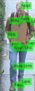
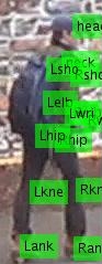
For appearance feature, we use an HSV (hue, saturation, value) color histogram for upper and lower body parts where the bin size is 16, 4 and 4 for Hue, Saturation and Value channels respectively. Furthermore, to capture the pose variations of a person, we use the Convolutional Pose Machinewei2016cpm to estimate the pose of a given image patch of a person. The estimated pose of a person is depicted in Figure 4a. To extract the upper body part, four joints(right shoulder, right hip, left shoulder, left hip) are used(Figure 4b). Six joints(right hip, right knee, right ankle, left hip, left knee, left ankle) are used for the bottom part of the body (Figure 4c). Once those body parts are extracted from an image patch, an HSV histogram, , is computed.
Even though we have used color histogram as the appearance feature and simple averaging model in this work, other online appearnce model can be applied to proposed MHT method since it is known that MHT can be extended by including online learned discriminative models without difficulty mht-rv.
4.2 DukeMTMC dataset
| Cam | method | ID-Measure | CLEAR MOT | |||||||||
| IDF1 | IDP | IDR | MOTA | MOTP | FAF | MT | ML | FP | FN | IDs | ||
| 1 | ristani2016MTMC | 57.3 | 91.2 | 41.8 | 43.0 | 79.0 | 0.03 | 24 | 46 | 2,713 | 107,178 | 39 |
| tesfaye2017multi | 76.9 | 89.1 | 67.7 | 69.9 | 76.3 | 0.06 | 137 | 22 | 5,809 | 52,152 | 156 | |
| Ours | 84.3 | 89.7 | 79.6 | 84.9 | 79.5 | 0.04 | 191 | 12 | 3,679 | 25,318 | 55 | |
| 2 | ristani2016MTMC | 68.0 | 69.3 | 67.1 | 44.8 | 78.2 | 0.51 | 133 | 8 | 47,919 | 5,374 | 60 |
| tesfaye2017multi | 81.2 | 90.9 | 73.4 | 71.5 | 74.6 | 0.09 | 134 | 21 | 8,487 | 43,912 | 75 | |
| Ours | 81.9 | 88.9 | 75.9 | 78.4 | 77.1 | 0.07 | 151 | 8 | 6,390 | 33,377 | 81 | |
| 3 | ristani2016MTMC | 60.3 | 78.9 | 48.8 | 57.8 | 77.5 | 0.02 | 52 | 22 | 1,438 | 28,692 | 16 |
| tesfaye2017multi | 64.6 | 76.3 | 56.0 | 67.4 | 75.6 | 0.02 | 44 | 9 | 2,148 | 21,125 | 38 | |
| Ours | 69.3 | 76.2 | 63.5 | 65.7 | 77.0 | 0.06 | 58 | 7 | 5,908 | 18,589 | 22 | |
| 4 | ristani2016MTMC | 73.5 | 88.7 | 62.8 | 63.2 | 80.2 | 0.02 | 36 | 18 | 2,209 | 19,323 | 7 |
| tesfaye2017multi | 84.7 | 91.2 | 79.0 | 76.8 | 76.6 | 0.03 | 45 | 4 | 2,860 | 10,686 | 18 | |
| Ours | 80.7 | 84.1 | 77.6 | 79.8 | 80.1 | 0.04 | 47 | 3 | 3,633 | 8,173 | 17 | |
| 5 | ristani2016MTMC | 73.2 | 83.0 | 65.4 | 72.8 | 80.4 | 0.05 | 107 | 17 | 4,464 | 35,861 | 54 |
| tesfaye2017multi | 68.3 | 76.1 | 61.9 | 68.9 | 77.4 | 0.10 | 88 | 11 | 9,117 | 36,933 | 139 | |
| Ours | 73.7 | 81.4 | 67.3 | 76.6 | 80.0 | 0.05 | 110 | 8 | 4,410 | 30,195 | 83 | |
| 6 | ristani2016MTMC | 77.2 | 84.5 | 69.1 | 73.4 | 80.2 | 0.06 | 142 | 27 | 5,279 | 45,170 | 55 |
| tesfaye2017multi | 82.7 | 91.6 | 75.3 | 77.0 | 77.2 | 0.05 | 136 | 11 | 4,868 | 38,611 | 142 | |
| Ours | 83.5 | 88.9 | 78.8 | 82.8 | 80.2 | 0.06 | 163 | 6 | 5,478 | 27,194 | 69 | |
| 7 | ristani2016MTMC | 80.5 | 93.6 | 70.6 | 71.4 | 74.7 | 0.02 | 69 | 13 | 1,395 | 18,904 | 23 |
| tesfaye2017multi | 81.6 | 94.0 | 72.5 | 73.8 | 74.0 | 0.01 | 64 | 4 | 1,182 | 17,411 | 36 | |
| Ours | 81.5 | 91.4 | 73.5 | 77.0 | 75.5 | 0.01 | 69 | 7 | 1,232 | 15,119 | 33 | |
| 8 | ristani2016MTMC | 72.4 | 92.2 | 59.6 | 60.7 | 76.7 | 0.03 | 102 | 53 | 2,730 | 52,806 | 46 |
| tesfaye2017multi | 73.0 | 89.1 | 61.0 | 63.4 | 73.6 | 0.04 | 92 | 28 | 4,184 | 47,565 | 91 | |
| Ours | 79.9 | 90.8 | 71.3 | 71.6 | 75.3 | 0.05 | 125 | 21 | 4,850 | 35,288 | 46 | |
| Single Cam Average | ristani2016MTMC | 70.1 | 83.6 | 60.4 | 59.4 | 78.7 | 0.09 | 665 | 234 | 68,147 | 361,672 | 91 |
| tesfaye2017multi | 77.0 | 87.6 | 68.6 | 70.9 | 75.8 | 0.05 | 740 | 110 | 38,655 | 268,398 | 693 | |
| Ours | 80.3 | 87.3 | 74.4 | 78.3 | 78.4 | 0.05 | 914 | 72 | 35,580 | 193,253 | 406 | |
| Multi-Cam | ristani2016MTMC | 56.2 | 67.0 | 48.4 | ||||||||
| tesfaye2017multi | 60.0 | 68.3 | 53.5 | |||||||||
| Ours | 65.4 | 71.1 | 60.6 | |||||||||
The DukeMTMC is a large, fully-annotated, calibrated dataset that captures the campus of Duke University, and was recorded using eight fixed cameras. The dataset has an RoI (region of interest) area for each camera where an evaluation is made. The topology of the fixed cameras is shown in Figure 5 where there is no field overlap between any pair of cameras(Figure 5b). The cameras used to acquire the dataset were synchronized and recorded at 1080p resolution and 60fps. The dataset contains more than 7,000 single camera trajectories and over 2,000 unique identities captures during minutes of recording for each camera, thus, a total of more than 10 h. The video was split into one training/validation set and two test sets, test-easy and test-hard set. The difficulty of the test-easy set is similar to the training/validation set, and it is 25 minutes long. The test-hard set is 10 minute-long videos and contains a group of dozens of people traversing multiple cameras.
The evaluation criteria for the DukeMTMC dataset is ID-Measure ristani2016MTMC, which measures how well a tracker determine who is where at all times. This criteria has three measures: IDP (Identification precision), IDR (Identification Recall), and IDF1 (Identification F-Score). The IDP (IDR) is the fraction of computed (ground truth) detections that are correctly identified. IDF1 is the ratio of correctly identified detections over the average number of ground-truth and computed detections. This process is different from CLEAR MOTBernardin2008, which reports the amount of incorrect decisions made by a tracker. Moreover unlike CLEAR MOT, it can measure not only the single camera tracking results but also the multi-camera tracking results. We reported the single camera tracking performance with both ID-Measure and CLEAR MOT in order to make it clear how much proposed method improved the final tracking performance given these single camera tracks.


We compared the quantitative performance of our method with other multi-target multi-camera tracking methodsristani2016MTMC; tesfaye2017multi using the DukeMTMC dataset. The results are shown in Table 2 and Table 3. The evaluation on the Test-easy is shown in Table 2, while the performance on the Test-hard is shown in Table 3. In both tables, the last row is for comparison of multi-camera tracking performance and the rest are for comparison of single camera tracking performance. We used public detection responses as the input to our method. The results of single camera tracking between ours and ristani2016MTMC were different, even though we used the public single camera tracker that is published by E. Ristani et al.ristani2014tracking, because we modified the original one to fit our multi-camera tracking method.11
1
The modified version of ristani2014tracking is currently on the web.
https://github.com/yoon28/SCT4DukeMTMC/
The last row of Table 2 shows that the performance of our multi-camera tracking method outperformed the state-of-the-art methodtesfaye2017multi on the Test-easy sequence by in IDF1, in IDP and in IDR metrics. In the Test-hard sequence, the proposed method ranked second with difference of in IDF1 and in IDP metrics, while it was first in IDR metrics (improvement of , Table 3). Finally, the proposed MHT algorithm for the multi-camera tracking method outperformed the method of ristani2016MTMC even in the complicated video sequence(Test-hard). Even if the ristani2016MTMC’s average IDF1 over single cameras was higher than ours by , the IDF1 of their multi-camera tracking performance was even lower than ours by (Table 3).
| Cam | method | ID-Measure | CLEAR MOT | |||||||||
| IDF1 | IDP | IDR | MOTA | MOTP | FAF | MT | ML | FP | FN | IDs | ||
| 1 | ristani2016MTMC | 52.7 | 92.5 | 36.8 | 37.8 | 78.1 | 0.03 | 6 | 34 | 1,257 | 78,977 | 55 |
| tesfaye2017multi | 67.1 | 83.0 | 56.4 | 63.2 | 75.7 | 0.08 | 65 | 17 | 2,886 | 44,253 | 408 | |
| Ours | 64.6 | 72.2 | 58.4 | 61.1 | 76.7 | 0.35 | 78 | 11 | 12,570 | 37,287 | 394 | |
| 2 | ristani2016MTMC | 60.6 | 65.7 | 56.1 | 47.3 | 76.5 | 0.74 | 68 | 12 | 26,526 | 46,898 | 194 |
| tesfaye2017multi | 63.4 | 78.8 | 53.1 | 54.8 | 73.9 | 0.24 | 62 | 16 | 8,653 | 54,252 | 323 | |
| Ours | 56.6 | 61.2 | 52.6 | 50.4 | 74.4 | 0.68 | 66 | 10 | 24,591 | 44,401 | 392 | |
| 3 | ristani2016MTMC | 62.7 | 96.1 | 46.5 | 46.7 | 77.9 | 0.01 | 24 | 4 | 288 | 18,182 | 6 |
| tesfaye2017multi | 81.5 | 91.1 | 73.7 | 68.8 | 75.1 | 0.06 | 18 | 2 | 2,093 | 8,701 | 11 | |
| Ours | 80.0 | 86.9 | 74.1 | 70.3 | 76.8 | 0.07 | 22 | 2 | 2,543 | 7,737 | 10 | |
| 4 | ristani2016MTMC | 84.3 | 86.0 | 82.7 | 85.3 | 81.5 | 0.04 | 21 | 0 | 1,215 | 2,073 | 1 |
| tesfaye2017multi | 82.3 | 87.1 | 78.1 | 75.6 | 77.7 | 0.05 | 17 | 0 | 1,571 | 3,888 | 61 | |
| Ours | 83.3 | 84.4 | 82.2 | 81.2 | 81.6 | 0.05 | 20 | 1 | 1,821 | 2,404 | 1 | |
| 5 | ristani2016MTMC | 81.9 | 90.1 | 75.1 | 78.3 | 80.7 | 0.04 | 57 | 2 | 1,480 | 11,568 | 13 |
| tesfaye2017multi | 82.8 | 91.5 | 75.7 | 78.6 | 76.7 | 0.03 | 47 | 2 | 1,219 | 11,644 | 50 | |
| Ours | 85.7 | 93.3 | 79.2 | 81.9 | 80.1 | 0.02 | 52 | 2 | 875 | 10,017 | 24 | |
| 6 | ristani2016MTMC | 64.1 | 81.7 | 52.7 | 59.4 | 76.7 | 0.14 | 85 | 23 | 5,156 | 77,031 | 225 |
| tesfaye2017multi | 53.1 | 71.2 | 42.3 | 53.3 | 76.5 | 0.17 | 68 | 36 | 5,989 | 88,164 | 547 | |
| Ours | 54.7 | 70.0 | 44.9 | 56.1 | 77.8 | 0.22 | 82 | 24 | 7,902 | 80,716 | 423 | |
| 7 | ristani2016MTMC | 59.6 | 81.2 | 47.1 | 50.8 | 73.3 | 0.08 | 43 | 23 | 2,971 | 38,912 | 148 |
| tesfaye2017multi | 60.6 | 84.7 | 47.1 | 50.8 | 74.0 | 0.05 | 34 | 20 | 1,935 | 39,865 | 266 | |
| Ours | 55.7 | 74.7 | 44.4 | 49.8 | 73.8 | 0.11 | 42 | 25 | 4,405 | 38,687 | 214 | |
| 8 | ristani2016MTMC | 82.4 | 94.9 | 72.8 | 73.0 | 75.9 | 0.02 | 34 | 5 | 706 | 9,735 | 10 |
| tesfaye2017multi | 81.3 | 90.3 | 73.9 | 70.0 | 72.6 | 0.06 | 37 | 6 | 2,297 | 9,306 | 26 | |
| Ours | 80.4 | 93.5 | 70.5 | 71.5 | 74.0 | 0.02 | 38 | 5 | 731 | 10,278 | 10 | |
| Single Cam Average | ristani2016MTMC | 64.5 | 81.2 | 53.5 | 54.6 | 77.1 | 0.14 | 338 | 103 | 39,599 | 283,376 | 652 |
| tesfaye2017multi | 65.4 | 81.4 | 54.7 | 59.6 | 75.4 | 0.09 | 348 | 99 | 26,643 | 260,073 | 1637 | |
| Ours | 63.5 | 73.9 | 55.6 | 59.6 | 76.7 | 0.19 | 400 | 80 | 55,038 | 231,527 | 1468 | |
| Multi-Cam | ristani2016MTMC | 47.3 | 59.6 | 39.2 | ||||||||
| tesfaye2017multi | 50.9 | 63.2 | 42.6 | |||||||||
| Ours | 50.1 | 58.3 | 43.9 | |||||||||
4.3 NLPR_MCT dataset

The NLPR_MCT dataset consists of four sub-datasets. A sub-dataset is depicted in Figure 622 2 This figure is captured from http://mct.idealtest.org/. Each sub-dataset includes 3-5 cameras with non-overlapping scenes and recordes different situations according to the number of people (ranging from 14 to 255) and the level of illumination changes and occlusionsmct2014. The videos contain both real scenes and simulated environments. Each video was nearly 20 minutes long (except Dataset 3), with a rate of 25 fps.
In this dataset, the topological connection information for every pair of entry/exit points for each sub-dataset is provided. We split the of an observation into and , that represent the entry point and exit point of observation , respectively. Because the dataset did not provide separate training and test datasets, we learned the parameters for our method as well as the transition matrix, the mean and standard deviation of transition time for each possible transition pair of entry/exit points using first 70 percent of each dataset.
The evaluation criteria used for the NLPR_MCT dataset was MCTA mct2014, multi-camera object tracking accuracy. It was modified based on CLEAR MOT Bernardin2008 and can be applied to MCT. The metric contains three terms (detection ability, single camera tracking ability and MCT ability), which are multiplied to produce one measure. In this experiment, we used annotated single camera trajectories by assuming that SCT problem is solved in advance33 3 This setting is identical to Experiment of MCT challenge. . We compared the performance of our method with the state-of-the-art methods in Table 4. The last column, Avg. Rank, is the averaged ranking over four sub-datasets, where the rank was decided by the MCTA score. This criterion is also used in MCT challenge to compare the results with others. The first place for each sub-dataset was shown in boldface. As a result, both cai2014exploring and our method tied for second place by the Avg. Rank of . However, it is worth noticing that our method has more stable performance than that of cai2014exploring because the rank standard deviation of our method over all sub-datasets is while the standard deviation of cai2014exploring is . Again, the MCTA standard deviation of our method over all sub-datasets is while that of cai2014exploring is .
| Method | NLPR 1 | NLPR 2 | NLPR 3 | NLPR 4 | Avg. Rank |
| USC_Visioncai2014exploring | 0.9152 | 0.9132 | 0.5162 | 0.7051 | 3.5 |
| UW_IPLlee2017online | 0.9610 | 0.9265 | 0.7889 | 0.7578 | 1.25 |
| CRF_UCRchen2016integrating | 0.8383 | 0.8015 | 0.6645 | 0.7266 | 3.75 |
| EGTrackermct2014 | 0.8353 | 0.7034 | 0.7417 | 0.3845 | 4.75 |
| DukeMTMCristani2016MTMC | 0.7967 | 0.7336 | 0.6543 | 0.7616 | 4.25 |
| Ours | 0.9129 | 0.8944 | 0.6699 | 0.6812 | 3.5 |
used for evaluation.
4.4 N-scan Pruning
In this section, we report how our MHT algorithm is sensitive to the parameter of -scan pruning. The -scan pruning algorithm assumes that any ambiguity at is resolved by time . The -scan pruning was utilized in the multi-scan assignment approach to MHT because it solves the data association problems with recent scans of the data thanks to -scan pruningblackman-book; poore1993data. We evaluated the ID-Measure for various , , on the Trainval-Mini of the DukeMTMC dataset. The Trainval-Mini is a small part of the training/validation set of the DukeMTMC dataset and is about 18 minutes long sequence. The parameter settings were the same as before except the . The intersection-over-union is fixed to for this experiment. The experimental result is shown in Figure 7. The result demonstrates that our MHT algorithm is negatively affected by in IDP while it is slightly positively affected in IDR when is increasing. Therefore, the proposed method has a small sensitivity to in terms of IDF1 because the IDP and the IDR are negatively correlated with respect to the . The difference between the minimum(58.02%) and maximum(58.87%) values in IDF1 was 0.85%. The minimum and maximum value of IDP was 64.97% and 66.57%, respectively, while that of IDR was 51.98% and 53.08%, respectively.
4.5 Real-time implementation
In this section, a real-time implementation of the proposed method is described. Full implementation of the proposed method was programmed by Matlab with a desktop PC(Intel i7-4790K 4.0 Ghz 4-core CPU, 16GB RAM, Nvidia GTX 770 GPU and Ubuntu 16.04 OS). For the computation efficiency, we have discarded the Convolutional Pose Machine in the appearance modeling and switched the SCT algorithm from ristani2014tracking to GM-PHD(Gaussian Mixture Probability Hypothesis Density) filtersong2016online for real-time implementation. There was no other reasons for switching the SCT algorithm except that we had already implemented the GMPHD in C++. Real-time implementation was developed using Visual C++ with the multi-thread programming and OpenCV in Windows 10 OS. The test hardware environment included a PC with Intel i7-7700K 4.5 Ghz 4-core CPU, 32GB RAM. To test the processing speed, we have generated a new dataset consisting of six videos with resolution and about 7 minutes long(Figure 8). This dataset, which includes appearance of up to 25 targets, was recorded in the campus of Gwangju Institute of Science and Technology. To detect a person in the dataset, we applied the pedestrian detectorkudet, which processes every frame of each camera to detect pedestrians. The average processing time (includes the processing time of detection, SCT and MCT) was about 15 frames per second for all videos. Note that each video(camera) was processed in parallel by multi-thread programming. Therefore, this result demonstrates the real-time performance of our method. We used the Gurobi optimizer to solve MWIS problems in this implementations.
5 Conclusion
In this paper, we applied a multiple hypothesis tracking algorithm to handle the multi-target multi-camera tracking problem with disjoint views. Our method forms track-hypothesis trees whose branch represents a multi-camera track which describes the trajectory of a target that may move within a camera as well as move across cameras. Furthermore, tracking targets within a camera is performed simultaneously with the tree formation by manipulating a status of each track hypothesis. Besides, two gating schemes have been proposed to differentiate the tracking scenarios. The experimental results shows that our method achieves state-of-the-art performance on DukeMTMC dataset and performs comparable to the state-of-the-art method on NLPR_MCT dataset. We also show that the proposed method can solve the problem under online and real-time conditions, provided that the single camera tracker solves in such conditions as well.
MHT can be extended by including online learned discriminative appearance models for each track hypothesismht-rv. Therefore, as for the future work, we will investigate online learning techniques that could learn a model for each hypothesis since we used a simple averaging model for appearance modeling in this work.
6 Acknowledgement
This work was supported by Institute for Information and communications Technology Promotion(IITP) grant funded by the Korea government(MSIP) (No. B0101-15-0525, Development of global multi-target tracking and event prediction techniques based on real-time large-scale video analysis). In addition, this work also supported by Korea Creative Content Agency (KOCCA) and Ministry of Culture, Sports and Tourism (MCST) (No. R2017050052, Developed intelligent UI/UX technology for AR glasses-based docent operation).


References
- [1] X. Chen, K. Huang, and T. Tan, “Object tracking across non-overlapping views by learning inter-camera transfer models,” Pattern Recognition, vol. 47, no. 3, pp. 1126–1137, 2014.
- [2] O. Javed, Z. Rasheed, K. Shafique, and M. Shah, “Tracking across multiple cameras with disjoint views,” in Proceedings of the Ninth IEEE International Conference on Computer Vision-Volume 2, p. 952, IEEE Computer Society, 2003.
- [3] Y. Wang, S. Velipasalar, and M. C. Gursoy, “Distributed wide-area multi-object tracking with non-overlapping camera views,” Multimedia tools and applications, vol. 73, no. 1, pp. 7–39, 2014.
- [4] Y. T. Tesfaye, E. Zemene, A. Prati, M. Pelillo, and M. Shah, “Multi-target tracking in multiple non-overlapping cameras using constrained dominant sets,” arXiv preprint arXiv:1706.06196, 2017.
- [5] E. Ristani and C. Tomasi, “Tracking multiple people online and in real time,” in Asian Conference on Computer Vision, pp. 444–459, Springer, 2014.
- [6] S.-E. Wei, V. Ramakrishna, T. Kanade, and Y. Sheikh, “Convolutional pose machines,” in Proceedings of the IEEE Conference on Computer Vision and Pattern Recognition, pp. 4724–4732, 2016.
- [7] X. Wang, E. Türetken, F. Fleuret, and P. Fua, “Tracking interacting objects using intertwined flows,” IEEE transactions on pattern analysis and machine intelligence, vol. 38, no. 11, pp. 2312–2326, 2016.
- [8] J. Berclaz, F. Fleuret, E. Turetken, and P. Fua, “Multiple object tracking using k-shortest paths optimization,” IEEE transactions on pattern analysis and machine intelligence, vol. 33, no. 9, pp. 1806–1819, 2011.
- [9] L. Zhang, Y. Li, and R. Nevatia, “Global data association for multi-object tracking using network flows,” in Computer Vision and Pattern Recognition, 2008. CVPR 2008. IEEE Conference on, pp. 1–8, IEEE, 2008.
- [10] H. Pirsiavash, D. Ramanan, and C. C. Fowlkes, “Globally-optimal greedy algorithms for tracking a variable number of objects,” in Computer Vision and Pattern Recognition (CVPR), 2011 IEEE Conference on, pp. 1201–1208, IEEE, 2011.
- [11] R. T. Collins, “Multitarget data association with higher-order motion models,” in Computer Vision and Pattern Recognition (CVPR), 2012 IEEE Conference on, pp. 1744–1751, IEEE, 2012.
- [12] C. Kim, F. Li, A. Ciptadi, and J. M. Rehg, “Multiple hypothesis tracking revisited,” in Proceedings of the IEEE International Conference on Computer Vision, pp. 4696–4704, 2015.
- [13] I. J. Cox and S. L. Hingorani, “An efficient implementation of reid’s multiple hypothesis tracking algorithm and its evaluation for the purpose of visual tracking,” IEEE Transactions on pattern analysis and machine intelligence, vol. 18, no. 2, pp. 138–150, 1996.
- [14] D. Papageorgiou and M. Salpukas, “The maximum weight independent set problem for data association in multiple hypothesis tracking,” Optimization and Cooperative Control Strategies, pp. 235–255, 2009.
- [15] S. Oh, S. Russell, and S. Sastry, “Markov chain monte carlo data association for multi-target tracking,” IEEE Transactions on Automatic Control, vol. 54, no. 3, pp. 481–497, 2009.
- [16] D. Reid, “An algorithm for tracking multiple targets,” IEEE transactions on Automatic Control, vol. 24, no. 6, pp. 843–854, 1979.
- [17] Y.-m. Song and M. Jeon, “Online multiple object tracking with the hierarchically adopted gm-phd filter using motion and appearance,” in Consumer Electronics-Asia (ICCE-Asia), IEEE International Conference on, pp. 1–4, IEEE, 2016.
- [18] O. Javed, K. Shafique, Z. Rasheed, and M. Shah, “Modeling inter-camera space–time and appearance relationships for tracking across non-overlapping views,” Computer Vision and Image Understanding, vol. 109, no. 2, pp. 146–162, 2008.
- [19] B. J. Prosser, S. Gong, and T. Xiang, “Multi-camera matching using bi-directional cumulative brightness transfer functions.,” in BMVC, p. 74, 2008.
- [20] A. Gilbert and R. Bowden, “Tracking objects across cameras by incrementally learning inter-camera colour calibration and patterns of activity,” Computer Vision–ECCV 2006, pp. 125–136, 2006.
- [21] S. Srivastava, K. K. Ng, and E. J. Delp, “Color correction for object tracking across multiple cameras,” in Acoustics, Speech and Signal Processing (ICASSP), 2011 IEEE International Conference on, pp. 1821–1824, IEEE, 2011.
- [22] C.-H. Kuo, C. Huang, and R. Nevatia, “Inter-camera association of multi-target tracks by on-line learned appearance affinity models,” in European Conference on Computer Vision, pp. 383–396, Springer, 2010.
- [23] S. Zhang, Y. Zhu, and A. Roy-Chowdhury, “Tracking multiple interacting targets in a camera network,” Computer Vision and Image Understanding, vol. 134, pp. 64–73, 2015.
- [24] L. Chen, H. Yang, J. Zhu, Q. Zhou, S. Wu, and Z. Gao, “Deep spatial-temporal fusion network for video-based person re-identification,” in Computer Vision and Pattern Recognition Workshops (CVPRW), 2017 IEEE Conference on, pp. 63–70, IEEE, 2017.
- [25] C.-W. Wu, M.-T. Zhong, Y. Tsao, S.-W. Yang, Y.-K. Chen, and S.-Y. Chien, “Track-clustering error evaluation for track-based multi-camera tracking system employing human re-identification,” in Computer Vision and Pattern Recognition Workshops (CVPRW), 2017 IEEE Conference on, pp. 1416–1424, IEEE, 2017.
- [26] S. Blackman and R. Popoli, “Design and analysis of modern tracking systems(book),” Norwood, MA: Artech House, 1999., 1999.
- [27] P. F. Felzenszwalb, R. B. Girshick, D. McAllester, and D. Ramanan, “Object detection with discriminatively trained part-based models,” IEEE transactions on pattern analysis and machine intelligence, vol. 32, no. 9, pp. 1627–1645, 2010.
- [28] B. D. Lucas and T. Kanade, “An iterative image registration technique with an application to stereo vision,” in Seventh Int’l Joint Conf. on Artificial Intelligence, pp. 674–679, Vancouver, BC, Canada, 1981.
- [29] A. Poore, N. Rijavec, M. Liggins, and V. Vannicola, “Data association problems posed as multidimensional assignment problems: problem formulation,” in Optical Engineering and Photonics in Aerospace Sensing, pp. 552–563, International Society for Optics and Photonics, 1993.
- [30] E. Ristani, F. Solera, R. Zou, R. Cucchiara, and C. Tomasi, “Performance measures and a data set for multi-target, multi-camera tracking,” in European Conference on Computer Vision, pp. 17–35, Springer, 2016.
- [31] W. Chen, L. Cao, X. Chen, and K. Huang, “An equalised global graphical model-based approach for multi-camera object tracking,” IEEE Transactions on Circuits and Systems for Video Technology (TCSVT), 2016.
- [32] K. Bernardin and R. Stiefelhagen, “Evaluating multiple object tracking performance: The clear mot metrics,” EURASIP Journal on Image and Video Processing, vol. 2008, p. 246309, May 2008.
- [33] Y. Cai and G. Medioni, “Exploring context information for inter-camera multiple target tracking,” in Applications of Computer Vision (WACV), 2014 IEEE Winter Conference on, pp. 761–768, IEEE, 2014.
- [34] Y.-G. Lee, Z. Tang, and J.-N. Hwang, “Online-learning-based human tracking across non-overlapping cameras,” IEEE Transactions on Circuits and Systems for Video Technology, 2017.
- [35] X. Chen and B. Bhanu, “Integrating social grouping for multi-target tracking across cameras in a crf model,” IEEE Transactions on Circuits and Systems for Video Technology, 2016.
- [36] H. K. W. P. J.Y. Kim, S.W. Kim and S. Ko, “Improved pedestrian detection using joint aggregated channel features,” in ICEIC, pp. 92–93, January 2016.