Evaluation Function Approximation for Scrabble

Scrabble[1] is a board game, where two players alternate on forming words on a 15x15 board by placing tiles bearing a single letter onto a board. The tiles must form words which, in crossword fashion, read left to right in rows or downwards in columns, and be defined in a standard dictionary or lexicon. Also, at least one of the tiles must be placed next to an existing tile on the board. The board is also marked with “premium” squares, which multiply the number of points awarded for a given word.

The game begins with a total of 100 tiles, placed in a bag in which the letters are invisible. The set of tiles that a player holds is called the rack and each player starts off with drawing seven tiles each from the bag. The set of tiles left after a player has moved is called the rack leave and for every letter placed on the board a replacement is drawn from the bag. The game ends when one player is out of tiles and no tiles are left to draw, or both players pass. The interested reader can find more details about the rules of Scrabble here.

Scrabble is a game of imperfect information, i.e. the current player is unaware about the rack of the opponent player, making it very hard to guess the opponent’s next move until the end of the game. Also, there is inherent randomness present in Scrabble as random letters are drawn from the bag to the current player’s rack at each round. The state space in Scrabble is also quite complex due to the tiles being marked with specific letters as opposed to being black and white. All these factors contribute to the difficulty of creating a perfect AI agent for Scrabble.

As a prerequisite to begin our exposition, we provide an overview of current state-of-the-art Scrabble agents with an high level description of the techniques employed in these agents in Chapter 2. Chapter 3 provides a detailed discussion of our approach towards the improving the evaluation function using black-box optimization methods. In Chapter 4, we shed light on our current framework involving supervised learning for approaching the problem. We conclude with a brief page of summary and directions for future work in Chapter 5.

Maven’s[2] game play is sub-divided into 3 phases:

1. 1.

   Mid-game: This phase lasts from the beginning of the game up until there are 9 or fewer tiles left in the bag. In this phase, all possible moves from the given rack are generated followed by sorting using some simple heuristics. The most promising moves among these moves are evaluated using 2-ply Monte-Carlo simulation where both players are assumed to draw tiles from the bag in each turn, and are assumed to play the best move based on the aforementioned heuristics. The move which is evaluated to be best after the simulations is played during the game.

2. 2.

   Pre-endgame: This phase is almost similar to the mid-game phase and is designed to attempt to yield a good end-game situation.

3. 3.

   Endgame: During this phase, there are no tiles left in the bag and thus, Scrabble becomes a game of perfect information. Maven uses the $B^{\star}$ search algorithm to analyze the game tree during the endgame phase.

Quackle[3] uses a similar approach as used by Maven. Quackle’s heuristic function¹¹ 1 Henceforth, shall be referred to as the static evaluation function used in the mid-game phase is a sum of the move score and the value of the rack leave. This leave value is computed using a precomputed database: it favors both the chance of playing a Bingo on the next turn as well as leaves that garnered high scores when they appeared on a player’s rack in a large sample of Quackle versus Quackle games. The win-percentage of each move is estimated and the move with the best win-percentage is played. Figure 2.1 presents a high level flow chart of the algorithm used in Quackle.

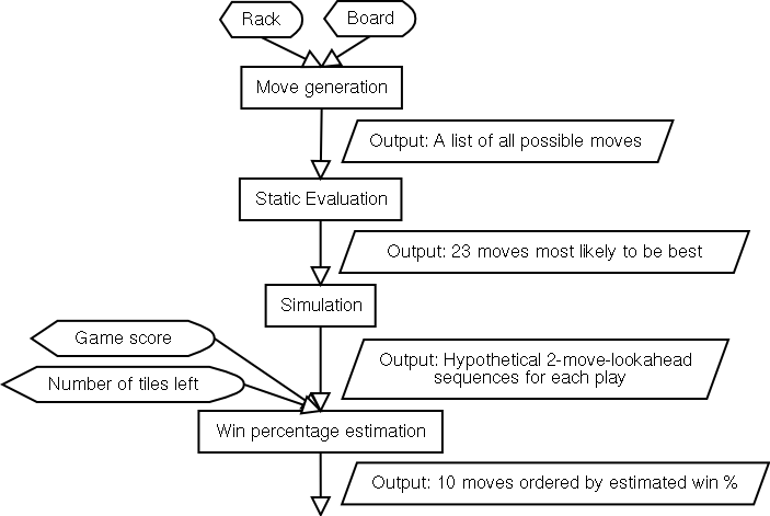
These are mainly two types of players present in the Quackle open source code which was used for our experiments:

1. 1.

   Speedy Player: The player only uses only static evaluations throughout the game and no Monte-Carlo simulations. The move predicted to be the best by the static evaluation function is played at a given board configuration.

2. 2.

   Championship Player: This player uses simulations in addition to static evaluations along with a perfect endgame player. This player can be provided with a particular amount of think-time²² 2 The win-rate of second player when the first player is a “Twenty Second Championship Player” i.e. it has a think-time of 20 seconds/move and the second player is a “Speedy Player” is $\approx\textbf{41.3\%}$ calculated using 50000 games. to run the truncated Monte-Carlo simulations for a single turn. For example, “Five Minute Championship Player” can take as long as five minutes to decide upon the move to play in a single turn.

Please note that the win-rate of second player when both players are Speedy Players is $\approx\textbf{43.8\%}$, calculated using 50000 self-play games.

We used an evolutionary algorithm[8], called CMA-ES (Covariance Matrix Adaptation Evolution Strategy)[9], to find the optimal weights for a feature-based evaluation function. An evolutionary algorithm is broadly based on the principle of biological evolution: In each generation, $\lambda$ new individuals are generated by stochastic variation of the current parental individuals. Then, the top $\mu$ individuals out of $\lambda$ are selected to become the parents in the next generation based on their fitness function value $f$. In this manner, over the generation sequence, individuals with better and better $f$-values are generated. Figure 3.1 presents a high level overview of the CMA-ES algorithm.

For our experiments, we ran 4-6 generations of CMA-ES with $\lambda=25$ and $\mu=13$ agents using the fitness function $f_{true}$ calculated through $N=50000$ self-play games between two “Speedy Players” as described in section 3.1.

Bayesian optimization[4] is a method of optimization of expensive cost functions without calculating derivatives. This kind of optimization employs the Bayesian technique of setting a prior over the objective function and combining it with evidence to get a posterior function. This allows an utility-based selection of the next observation using an acquisition function[11] that determines what the next query point should be. The acquisition function takes into account both sampling from areas of high uncertainty as well as areas likely to offer improvement over the current best observation.

Since our fitness functions are noisy (as only finite number of games are used to compute them), the idea of applying Bayesian optimization to find the optimal static evaluation function looked promising. However, this experiment also didn’t result in a significant improvement over the current win-rate of $43.8\%$ obtained by $e_{quackle}$.

Instead of using the same evaluation function for all stages⁴⁴ 4 Refer to section 2.1 for detailed information about the different phases. of the game, it seemed plausible to us that a combination of evaluation functions could work better for different game stages in Scrabble. This idea has been previously employed successfully in the game of Robot Soccer[12] and already been proposed in the context of Scrabble[13] as well. Keeping the evaluation function weights fixed for the early-game⁵⁵ 5 Early-game was defined as the phase of the game when the number of tiles in the bag were $\geq$ 80. and endgame phases, we only evolved the weights pertaining to the mid-game where the mid-game was defined to be the phase of game when the number of tiles in the bag were between 20 to 80. This experiment also proved to be futile and didn’t result in any improvement over the function $e_{quackle}$.

We initially experimented with a neural network approximator $G$ as the static evaluation function with input as a move represented by the various state-action features (including state-only features as well) described in section 3.2.2. We trained this neural network using a fixed dataset $D$ of state-action pairs with $\approx$ 70000 board configurations. For each board configuration $b$, the Quackle “Five Minute Championship Player” provides a sorted list $L_{b}$ of size min{10, $M_{b}$}, where $M_{b}$ is the list of all possible moves at configuration $b$. The dataset D is further split into training and validation datasets $D_{train}$ and $D_{val}$ with a ratio of 97:3.

Figure 4.1 presents the Rank-net[17] architecture for $G_{pair}$ which invokes the network $G$. For each board configuration $b$ in dataset $D$, the network $G_{pair}$ is provided with pair of moves ($L_{b}[1]$, $L_{b}[k]$) where $k\in\{2,3,..,|L_{b}|\}$ where L[i] denotes the $i^{th}$ element of the list $L$. The output label, $y_{output}=1$ for all such pairs. The binary cross-entropy loss function used for training is given by

However, results from this experiment were not very encouraging. The function approximator $G$ was only able to achieve a slightly better win-rate than $e_{quackle}$. Further, the validation accuracy achieved using the ranking loss was close to the baseline accuracy($\approx 73\%$) produced by $e_{quackle}$. We believe that the limited representation ability of the features used for this experiment was the limiting factor in this experiment.

The problem of designing good features for the game of Scrabble is quite important. The goodness of a board configuration depends both on spatial arrangement and on the presence or absence of sets of letters and ultimately needs consultation with the Scrabble dictionary as well. However, we think that combining these dimensions into a small number of discriminative signals is not an easy task. In order to tackle this problem, we decided to use the raw board representation of the Scrabble board as input to our evaluation function instead of using only a fixed number of hand-coded features.

AlphaGo Zero[18] used the raw board representation as input to neural networks trained using self-play and mastered the game of Go without using any human knowledge. Unlike Go, which only has white and black stones, Scrabble has 27 letters, each with a different value, and with combinations of letters having different a value from the sum of the constituents. This makes the Scrabble board a much harder proposition for a convolutional neural net(CNN[19])¹¹ 1 Henceforth, convolutional neural net is abbreviated as CNN to model well. However, given the enormous success of AlphaGo Zero, we decided to further investigate the idea of using raw board representations for Scrabble.

A $15\times 15$ Scrabble board $b$ is encoded into a $15\times 15\times 28$ feature vector $v(b)$ where the third dimension pertain to the different type of features used in our encoding of the Scrabble board. For a particular feature, each board position is a given a value. We used the following features for our encoding:

1. 1.

   Whether a position is blank or not

2. 2.

   Whether a position contains a particular alphabet, leading to a total of 26 features for the letters A-Z

3. 3.

   The score of the tile placed on a position. All positions not containing any tiles are given a score of zero except the premium scores which are given a score of -1.

The move at a given board configuration $b$ is provided as input using the concatenation of the feature vectors $v(b)$ and $v(b^{\prime})$ (let’s call it input1) where $b^{\prime}$ is the configuration obtained after playing the given move on $b$. In addition to input1, the two features used in $e_{quackle}$ (denoted by input2) also provided as input to our evaluation function. The neural network $G$ consists of many residual blocks[20] of convolutional layers with batch normalization[21] and ReLU activations and is trained in a similar manner as described by figure 4.1.

Specifically, $G$ consists of a single convolutional block followed by 2 residual blocks and a final block. The convolutional block applies the following modules sequentially to input1:

1. 1.

   A convolution of 16 filters of kernel size $3\times 3$ with stride 1

2. 2.

   Batch normalization

3. 3.

   A rectifier nonlinearity

Each residual block applies the following modules sequentially to its input:

1. 1.

   A convolution of 16 filters of kernel size $3\times 3$ with stride 1

2. 2.

   Batch normalization

3. 3.

   A rectifier nonlinearity

4. 4.

   A convolution of 16 filters of kernel size $3\times 3$ with stride 1

5. 5.

   Batch normalization

6. 6.

   A skip connection that adds the input to the block

7. 7.

   A rectifier nonlinearity

The final block applies the following modules sequentially to its input:

1. 1.

   A convolution of 1 filter of kernel size $1\times 1$ with stride 1

2. 2.

   Batch normalization

3. 3.

   A rectifier nonlinearity

4. 4.

   A fully connected linear layer to a hidden layer of size 32

5. 5.

   A rectifier nonlinearity

6. 6.

   A fully connected linear layer to a hidden layer of size 4

7. 7.

   A rectifier nonlinearity

8. 8.

   A concatenation layer which combines the previous layer input and input2

9. 9.

   A fully connected linear layer to a scalar

The number of weight parameters in $G$ were approximately 1/20 times the number of training example pairs used to train $G$.

Figure 4.2 shows the learning curves for the network $G$. This approach led to an validation accuracy of $\approx 85.4\%$ on $D_{val}$ which was not used for training. Given these initial results, this approach looks very promising and future work may involve exploring it further.

References

- [1] Wikipedia. Scrabble — wikipedia, the free encyclopedia, 2017. [Online; accessed 24-November-2017].
- [2] Brian Sheppard. World-championship-caliber scrabble. Artificial Intelligence, 134(1-2):241–275, 2002.
- [3] Jason Katz-Brown and John O’Laughlin. How quackle plays scrabble, 2005.
- [4] Eric Brochu, Vlad M Cora, and Nando De Freitas. A tutorial on bayesian optimization of expensive cost functions, with application to active user modeling and hierarchical reinforcement learning. arXiv preprint arXiv:1012.2599, 2010.
- [5] Wikipedia. Fitness function — wikipedia, the free encyclopedia, 2016. [Online; accessed 24-November-2017].
- [6] Wikipedia. Hoeffding’s inequality — wikipedia, the free encyclopedia, 2017. [Online; accessed 24-November-2017].
- [7] Emilie Kaufmann and Shivaram Kalyanakrishnan. Information complexity in bandit subset selection. In Conference on Learning Theory, pages 228–251, 2013.
- [8] William M Spears, Kenneth A De Jong, Thomas Bäck, David B Fogel, and Hugo De Garis. An overview of evolutionary computation. In European Conference on Machine Learning, pages 442–459. Springer, 1993.
- [9] Nikolaus Hansen. The cma evolution strategy: A tutorial. arXiv preprint arXiv:1604.00772, 2016.
- [10] Vinod Nair and Geoffrey E Hinton. Rectified linear units improve restricted boltzmann machines. In Proceedings of the 27th international conference on machine learning (ICML-10), pages 807–814, 2010.
- [11] Jasper Snoek, Hugo Larochelle, and Ryan P Adams. Practical bayesian optimization of machine learning algorithms. In Advances in neural information processing systems, pages 2951–2959, 2012.
- [12] Patrick MacAlpine, Daniel Urieli, Samuel Barrett, Shivaram Kalyanakrishnan, Francisco Barrera, Adrian Lopez-Mobilia, Nicolae Ştiurcă, Victor Vu, and Peter Stone. Ut austin villa 2011: A champion agent in the robocup 3d soccer simulation competition. In Proceedings of the 11th International Conference on Autonomous Agents and Multiagent Systems-Volume 1, pages 129–136. International Foundation for Autonomous Agents and Multiagent Systems, 2012.
- [13] Alejandro Romero, Rene Alquezar, Arturo Ramírez, Francisco González Acuña, and Ian García Olmedo. Human-like heuristics in scrabble. 202:381–390, 01 2009.
- [14] Ahmed Hussein, Mohamed Medhat Gaber, Eyad Elyan, and Chrisina Jayne. Imitation learning: A survey of learning methods. ACM Computing Surveys (CSUR), 50(2):21, 2017.
- [15] Brenna D Argall, Sonia Chernova, Manuela Veloso, and Brett Browning. A survey of robot learning from demonstration. Robotics and autonomous systems, 57(5):469–483, 2009.
- [16] David Silver, Aja Huang, Chris J Maddison, Arthur Guez, Laurent Sifre, George Van Den Driessche, Julian Schrittwieser, Ioannis Antonoglou, Veda Panneershelvam, Marc Lanctot, et al. Mastering the game of go with deep neural networks and tree search. Nature, 529(7587):484–489, 2016.
- [17] Chris Burges, Tal Shaked, Erin Renshaw, Ari Lazier, Matt Deeds, Nicole Hamilton, and Greg Hullender. Learning to rank using gradient descent. In Proceedings of the 22nd international conference on Machine learning, pages 89–96. ACM, 2005.
- [18] David Silver, Julian Schrittwieser, Karen Simonyan, Ioannis Antonoglou, Aja Huang, Arthur Guez, Thomas Hubert, Lucas Baker, Matthew Lai, Adrian Bolton, et al. Mastering the game of go without human knowledge. Nature, 550(7676):354–359, 2017.
- [19] Yann LeCun, Yoshua Bengio, and Geoffrey Hinton. Deep learning. Nature, 521(7553):436–444, 2015.
- [20] Kaiming He, Xiangyu Zhang, Shaoqing Ren, and Jian Sun. Deep residual learning for image recognition. In Proceedings of the IEEE conference on computer vision and pattern recognition, pages 770–778, 2016.
- [21] Sergey Ioffe and Christian Szegedy. Batch normalization: Accelerating deep network training by reducing internal covariate shift. In International Conference on Machine Learning, pages 448–456, 2015.
- [22] Christopher J Burges, Robert Ragno, and Quoc V Le. Learning to rank with nonsmooth cost functions. In Advances in neural information processing systems, pages 193–200, 2007.
- [23] Stéphane Ross, Geoffrey J Gordon, and Drew Bagnell. A reduction of imitation learning and structured prediction to no-regret online learning. In International Conference on Artificial Intelligence and Statistics, pages 627–635, 2011.