marginparsep has been altered.
topmargin has been altered.
marginparwidth has been altered.
marginparpush has been altered.
The page layout violates the ICML style.
Please do not change the page layout, or include packages like geometry, savetrees, or fullpage, which change it for you.
We’re not able to reliably undo arbitrary changes to the style. Please remove the offending package(s), or layout-changing commands and try again.
Fair -Center Clustering for Data Summarization
Matthäus Kleindessner 1 Pranjal Awasthi 1 Jamie Morgenstern 2
Abstract
In data summarization we want to choose prototypes in order to summarize a data set. We study a setting where the data set comprises several demographic groups and we are restricted to choose prototypes belonging to group . A common approach to the problem without the fairness constraint is to optimize a centroid-based clustering objective such as -center. A natural extension then is to incorporate the fairness constraint into the clustering problem. Existing algorithms for doing so run in time super-quadratic in the size of the data set, which is in contrast to the standard -center problem being approximable in linear time. In this paper, we resolve this gap by providing a simple approximation algorithm for the -center problem under the fairness constraint with running time linear in the size of the data set and . If the number of demographic groups is small, the approximation guarantee of our algorithm only incurs a constant-factor overhead.
1 Introduction
Machine learning (ML) algorithms have been rapidly adopted in numerous human-centric domains, from personalized advertising to lending to health care. Fast on the heels of this ubiquity have come a whole host of concerning behaviors from these algorithms: facial recognition has higher accuracy on white, male faces (Buolamwini & Gebru 2017); online advertisements suggesting arrest are shown more frequently to search queries that comprise a name primarily associated with minority groups (Sweeney 2013); and criminal recidivism tools are likely to mislabel black low-risk defendants as high-risk while mislabeling white high-risk defendants as low-risk (Angwin et al. 2016). There are also several examples of unsavory ML behavior pertaining to unsupervised learning tasks, such as gender stereotypes in word2vec embeddings (Bolukbasi et al. 2016). Most of the academic work on fairness in ML, however, has investigated how to solve classification tasks subject to various constraints on the behavior of a classifier on different demographic groups (Hardt et al. 2016; Zafar et al. 2017, e.g., ).
This paper adds to the literature on fair methods for unsupervised learning tasks (see Section 4 for related work). We consider the problem of data summarization (Hesabi et al. 2015) through the lens of algorithmic fairness. The goal of data summarization is to output a small but representative subset of a data set. Think of an image database and a user entering a query that is matched by many images. Rather than presenting the user with all matching images, we only want to show a summary. In such an example, a data summary can be quite unfair on a demographic group. Indeed, Google Images has been found to answer the query “CEO” with a much higher fraction of images of men compared to the real-world fraction of male CEOs (Kay et al. 2015).
One approach to the problem of data summarization is provided by centroid-based clustering, such as -center (formally defined in Section 2) or -medoid (Hastie et al. 2009, Section 14.3.10; sometimes referred to as -median). For a centroid-based clustering objective, an optimal clustering of a data set can be defined by points , called centroids, such that the clusters are formed by assigning every to its closest centroid. Since the centroids are good representatives of their clusters, the set of centroids can be used as a summary of . This approach of data summarization via centroid-based clustering is used in numerous domains, for example in text summarization (Moens et al. 1999) or robotics (Girdhar & Dudek 2012).
If the data set comprises several demographic groups , we may consider to be a fair summary only if the groups are represented fairly: if in the real world 70% of CEOs are male and we want to output ten images for the query “CEO”, then three of the ten images should show women. Formally, this can be encoded with one parameter for every group . Our goal is then to minimize the clustering objective under the constraint that many centroids belong to . A constraint of this form can also enforce balanced summaries: even if in the real world there are more male CEOs than female ones, we might want to output an equal number of male and female images to reflect that gender is not definitional to the role of CEO.
Centroid-based clustering under such a constraint has been studied in the theoretical computer science literature (see Sections 2 and 4). However, existing approximation algorithms for this problem run in time , while the unconstrained -center clustering problem can be approximated in time linear in . Since data summarization is particularly useful for massive data sets, such a slowdown may be practically prohibitive. The contribution of this paper is to present a simple approximation algorithm for -center clustering under our fairness constraint with running time only linear in and . The improved running time comes at the price of a worse guarantee on the approximation factor if the number of demographic groups is large. However, note that in practical situations concerning fairness, the number of groups is often quite small (e.g., when the groups encode gender or race). Furthermore, in our extensive numerical simulations we never observed a large approximation factor, even when the number of groups was large (cf. Section 5), indicating the practical usefulness of our algorithm.
Outline of the paper In Section 2, we formally state the -center and the fair -center problem. In Section 3, we present our algorithm and provide a sketch of its analysis. The full proofs can be found in Appendix A. We discuss related work in Section 4 and present a number of experiments in Section 5. Further experiments can be found in Appendix B. We conclude with a discussion in Section 6.
Notation For , we sometimes use .
2 Definition of -Center and Fair -Center
Let be a finite data set and be a metric on . In particular, we assume to satisfy the triangle inequality. The standard -center clustering problem is the minimization problem
| (1) |
where is a given parameter and . Here, are called centers. Any set of centers defines a clustering of by assigning every to its closest center. The -center problem is NP-hard and is also NP-hard to approximate to a factor better than (Gonzalez 1985; Vazirani 2001, Chapter 5). The famous greedy strategy of Gonzalez 1985 is a -approximation algorithm with running time if we assume that can be evaluated in constant time (this is the case, e.g., if a problem instance is given via the distance matrix ). This greedy strategy chooses an arbitrary element of the data set as first center and then iteratively selects the data point with maximum distance to the current set of centers as the next center to be added.
We consider a fair variant of the -center problem as described in Section 1. Our variant also allows for the user to specify a subset that has to be included in the set of centers (think of the example of the image database and the case that we always want to show five prespecified images as part of the summary). Assuming that , where are the demographic groups, the fair -center problem can be stated as the minimization problem
| (2) |
where with and are given. By means of a partition matroid, the fair -center problem can be phrased as a matroid center problem, for which Chen et al. 2016 provide a 3-approximation algorithm using matroid intersection (Cook et al. 1998, e.g., ). Chen et al. 2016 do not discuss the running time of their algorithm, but it requires to sort all distances between elements in and hence has running time at least . In our experiments in Section 5 we observe a running time in .
3 A Linear-time Approximation Algorithm
In this section, we present our approximation algorithm for the minimization problem (2). It is a recursive algorithm with respect to the number of groups . To increase comprehensibility, we first present the case of two groups and then the general case of an arbitrary number of groups.
At several points, we will consider the standard (unfair) -center problem (1) generalized to the case of initially given centers , that is
| (3) |
We can adapt the greedy strategy of Gonzalez 1985 for (1) to problem (3) while maintaining its 2-approximation guarantee. For the sake of completeness, we provide the algorithm as Algorithm 1 and state the following lemma:
Lemma 1.
A proof of Lemma 1, similar in structure to a proof in Har-Peled 2011 for the strategy of Gonzalez 1985 for problem (1), can be found in Appendix A.
3.1 Fair -Center with Two Groups
Assume that . Our algorithm first runs Algorithm 1 for the unfair problem (3) with and . If we are lucky and Algorithm 1 picks many centers from and many centers from , our algorithm terminates. Otherwise, Algorithm 1 picks too many centers from one group, say , and too few from . We try to decrease the number of centers in by replacing any such a center with an element in its cluster belonging to . Once we have made all such available swaps, the remaining clusters with centers in are entirely contained within . We then run Algorithm 1 on these clusters with and the centers from as well as as initially given centers, and return both the centers from the recursive call (all in ) and those from the initial call and the swapping in .
This algorithm is formally stated as Algorithm 2. The following theorem states that it is a 5-approximation algorithm and that our analysis is tight—in general, Algorithm 2 does not achieve a better approximation factor.
Theorem 1.
Proof.
Here we only present a sketch of the proof. The full proof can be found in Appendix A. For showing that Algorithm 2 is a 5-approximation algorithm, let be the optimal value of (2) and be the optimal value of (3) (for ). Clearly, . Let be the set of centers returned by Algorithm 2. It is clear that comprises many elements from and many elements from . We need to show that for every . Let be the output of Algorithm 1 when called in Line 3 of Algorithm 2. Since Algorithm 1 is a 2-approximation algorithm for (3) according to Lemma 1, we have , . Assume that . It follows from the triangle inequality that after exchanging centers in the while-loop in Line 9 of Algorithm 2 we have , . Assume that still . We only need to show that for . Let be an optimal solution to (2). We split into two subsets , where comprises all for which the closest center in is in . Using the triangle inequality we can show that , . We partition into at most many clusters corresponding to the closest center in . Each of these clusters has diameter not greater than . If Algorithm 1 in Line 15 of Algorithm 2 chooses one element from each of these clusters, we immediately have , . Otherwise, Algorithm 1 chooses an element from or two elements from the same cluster of . In both cases, it follows from the greedy choice property of Algorithm 1 that , .
A family of examples shows that Algorithm 2 is not a -approximation algorithm for any . ∎
3.2 Fair -Center with Arbitrary Number of Groups
The main idea to handle an arbitrary number of groups is the same as for the case : we first run Algorithm 1. We then exchange centers for elements in their clusters in such a way that the number of centers from a group comes closer to , which is the requested number of centers from . If via exchanging centers we can actually hit for every group , we are done. Otherwise, we wish that, when no more exchanging is possible, we are left with a subset that only comprises elements from or fewer groups. Denote the set of these groups by . We also wish that for those groups not in we have picked only the requested number of centers or fewer and we can consider the groups not in to have been “resolved”. If both are true, we can recursively apply our algorithm to and a smaller number of groups. We might recurse down to the case of only one group, which we can solve with Algorithm 1.
The difficulty with this idea comes from the exchanging process. Formally, we are given centers and the corresponding clustering , where is the union of clusters with a center in , and we want to exchange some centers for an element in their cluster such that there exists a strict subset of groups with the following properties:
| (4) | |||
| (5) |
While in the case of only two groups this can easily be achieved by exchanging centers from the group that has more than the requested number of centers for elements from the other group, as we do in Algorithm 2, it is not immediately clear how to deal with a situation as shown in Figure 1. There are three groups (elements of these groups are shown in blue, green, and red, respectively), and we have . For the current set of centers (elements at the centers of the circles) there does not exist satisfying (4) and (5). We would like to decrease the number of centers in and increase the number of centers in , but the clusters with a center in do not comprise an element from . Hence, we cannot directly exchange a center from for an element in . Rather, we first have to exchange a center from for an element in (although this increases the number of centers from over ) and then a center from for an element in . An algorithm that can deal with such a situation is Algorithm 3. It exchanges some centers for an element in their cluster and yields that provably satisfies (4) and (5), as stated by the following lemma. Its proof can be found in Appendix A.
Lemma 2.
Observing that the number of iterations of the while-loop in Line 7 is upper-bounded by as the proof of Lemma 2 shows, that the number of iterations of the for-loop in Line 8 is upper-bounded by , and that all shortest paths on can be computed in running time (Cormen et al. 2009, Chapter 25), it is not hard to see that Algorithm 3 can be implemented with running time .
Using Algorithm 3, it is straightforward to design a recursive approximation algorithm for the fair -center problem (2) as outlined at the beginning of Section 3.2. We state the algorithm as Algorithm 4. Applying, by means of induction, a similar technique as in the proof of Theorem 1 to every (recursive) call of Algorithm 4, we can prove the following:
- •
plays the role of
- •
we assign elements in to an arbitrary group in and hence there are many groups
- •
the requested numbers of centers are
- •
plays the role of initially given centers
Theorem 2.
It is not clear to us whether our analysis of Algorithm 4 is tight and the approximation factor achieved by Algorithm 4 can indeed be as large as or whether the dependence on is actually less severe (compare with Section 5 and Section 6). Although trying hard to find instances for which the approximation factor of Algorithm 4 is large, we never observed a factor greater than .
4 Related Work
Fairness By now, there is a huge body of work on fairness in machine learning. For a recent paper providing an overview of the literature on fair classification see Donini et al. 2018. Our paper adds to the literature on fair methods for unsupervised learning tasks (Chierichetti et al. 2017; Celis et al. 2018a; Celis et al. 2018b; Celis et al. 2018c; Samadi et al. 2018; Schmidt et al. 2018). Note that all these papers assume to know which demographic group a data point belongs to just as we do. We discuss the two works most closely related to our paper.
First, Celis et al. 2018b also deal with the problem of fair data summarization. They study the same fairness constraint as we do, that is the summary must contain many elements from group . However, while we aim for a representative summary, where every data point should be close to at least one center in the summary, Celis et al. 2018b aim for a diverse summary. Their approach requires the data set to consist of points in , and then the diversity of a subset of is measured by the volume of the parallelepiped that it spans (Kulesza & Taskar 2012). This summarization objective is different from ours, and in different applications one or the other may be more appropriate. An advantage of our approach is that it only requires access to a metric on the data set rather than feature representations of data points.
The second line of work we discuss centers around the paper of Chierichetti et al. 2017. Their paper proposes a notion of fairness for clustering different from ours. Based on the fairness notion of disparate impact (Feldman et al. 2015) / the -rule (Zafar et al. 2017) for classification, the paper by Chierichetti et al. 2017 asks that every group be approximately equally represented in each cluster. In their paper, Chierichetti et al. 2017 focus on -medoid and -center clustering and the case of two groups. Subsequently, Rösner & Schmidt 2018 study such a fair -center problem for multiple groups, and Schmidt et al. 2018 build upon the work of Chierichetti et al. 2017 to devise algorithms for such a fair -means problem. Kleindessner et al. 2019 incorporate the fairness notion of Chierichetti et al. 2017 into the spectral clustering framework. While we certainly consider the fairness notion of Chierichetti et al. 2017, which can be applied to any kind of clustering, to be meaningful in some scenarios, we believe that in certain applications of centroid-based clustering (such as data summarization) our proposed fairness notion provides a more sensible alternative.
Centroid-based clustering There are many papers proposing heuristics and approximation algorithms for both -center (Hochbaum & Shmoys 1986; Mladenović et al. 2003; Ferone et al. 2017, e.g., ) and -medoid (Charikar et al. 2002; Arya et al. 2004; Li & Svensson 2013, e.g.,) under various assumptions on and the distance function . There are also numerous papers on versions with constraints, such as lower or upper bounds on the size of the clusters (Aggarwal et al. 2010; Cygan et al. 2012; Rösner & Schmidt 2018).
Most important to mention are the works by Hajiaghayi et al. 2010, Krishnaswamy et al. 2011 and Chen et al. 2016. Hajiaghayi et al. 2010 are the first that consider our fairness constraint (for two groups) for -medoid. They present a local search algorithm and prove it to be a constant-factor approximation algorithm. Their work has been generalized by Krishnaswamy et al. 2011, who consider -medoid under the constraint that the centers have to form an independent set in a given matroid. This kind of constraint contains our fairness constraint as a special case (for an arbitrary number of groups). Krishnaswamy et al. 2011 obtain a 16-approximation algorithm for this so-called matroid median problem based on rounding the solution of a linear programming relaxation. Subsequently, Chen et al. 2016 study the matroid center problem. Using matroid intersection as black box, they obtain a 3-approximation algorithm. Note that none of Hajiaghayi et al. 2010, Krishnaswamy et al. 2011 or Chen et al. 2016 discuss the running time of their algorithm, except for arguing it to be polynomial (see Section 2). We also mention the works by Chakrabarty & Negahbani 2018, who provide a generalization of the matroid center problem and in doing so recover the result of Chen et al. 2016, and by Kale 2018, who studies the matroid center problem in a streaming setting.
5 Experiments
In this section, we present a number of experiments11 1 Python code is available on https://github.com/matthklein/fair_k_center_clustering.. We begin with a motivating example on a small image data set illustrating that a summary produced by Algorithm 1 (i.e., the standard greedy strategy for the unfair -center problem) can be quite unfair. We also compare summaries produced by our algorithm to summaries produced by the method of Celis et al. 2018b. We then investigate the approximation factor of our algorithm on several artificial instances with known or computable optimal value of the fair -center problem (2) and compare our algorithm to the one for the matroid center problem by Chen et al. 2016, both in terms of approximation factor / cost of output and running time. Next, on both synthetic and real data, we compare our algorithm in terms of the cost of its output to two baseline heuristics (with running time linear in and just as for our algorithm). Finally, we compare our algorithm to Algorithm 1 more systematically. We study the difference in the costs of the outputs of our algorithm and Algorithm 1, a quantity one may refer to as price of fairness, and measure how unfair the output of Algorithm 1 can be. In the following, all boxplots show results of 200 runs of an experiment.
5.1 Motivating Example and Comparison with Celis et al. 2018b

| Algorithm 1 | Our Algorithm | Celis et al. 2018b |
 |
 |
 |
Consider the 14 images22 2 All images were found on https://pexels.com, https://pixnio.com or https://commons.wikimedia.org and are in the public domain. of medical doctors shown in the first row of Figure 2. Assume we want to generate a summary of size four of these images. One way to do so is to run Algorithm 1. The first column of the table in Figure 2 shows in each row the summary produced in one run of Algorithm 1 (recall that all algorithms considered here are randomized algorithms). These summaries are quite unfair: although there is an equal number of images of female doctors and images of male doctors, all these summaries show three or even four females. To overcome this bias we can apply our algorithm or the method of Celis et al. 2018b, which both allow us to explicitly state the numbers of females and males that we want in the summary. The second and the third column of the table show summaries produced by these algorithms. It is hard to say which of them produces more useful summaries and the results ultimately depend on the feature representations of the images (see the next paragraph). To provide further illustration, we present a similar experiment in Figure 11 in Appendix B.

For computing feature representations of the images and running the algorithm of Celis et al. 2018b we used the code provided by them. The feature vector of an image is a histogram based on the image’s SIFT descriptors; see Celis et al. 2018b for details. We used the Euclidean metric between these feature vectors as metric for Algorithm 1 and our algorithm.
5.2 Approximation Factor and Comparison with Chen et al. 2016
We implemented the algorithm by Chen et al. 2016 using the generic algorithm for matroid intersection provided in SageMath33 3 http://sagemath.org/. To speed up computation, rather than testing all distance values as threshold as suggested by Chen et al. 2016, we implemented binary search to look for the optimal value.
In the experiment shown in the left part of Figure 3, we study the approximation factor achieved by our algorithm (Alg. 4) and the algorithm by Chen et al. 2016 (M.C.) in various settings of values of , and , . The data set always consists of 25 vertices of a random graph and is small enough to explicitly compute an optimal solution to the fair -center problem (2). The random graph is constructed according to an Erdős-Rényi model, where any possible edge between two vertices is contained in the graph with probability . With high probability such a graph is connected (if not, we discard it). We put random weights on the edges, drawn from the uniform distribution on , and let the metric be the shortest-path distance on the graph. We assign every vertex to one of groups uniformly at random and randomly choose a subset of initially given centers. As we can see from the boxplots, the approximation factor achieved by our algorithm is never larger than 2.2. We also see that in each of the seven settings that we consider the median of the achieved approximation factors (indicated by the red lines in the boxes) is smaller for our algorithm than for the algorithm by Chen et al. 2016.
In the experiment shown in the right part of Figure 3, we study the running time of the two algorithms as a function of the size of the data set, which is created analogously to the experiment in the left part. We set , and , . The shown curves are obtained from averaging the running times of 200 runs of the experiment (performed on an iMac with 3.4 GHz i5 / 8 GB DDR4). While our algorithm never runs for more than 0.01 seconds, the algorithm by Chen et al. 2016, on average, runs for 230 seconds when . Its run time grows at least as , which proves it to be inappropriate for massive data sets. Boxplots of the costs of the outputs obtained in this experiment are provided in Figure 9 in Appendix B. We can see there that the costs are very similar for the two algorithms.
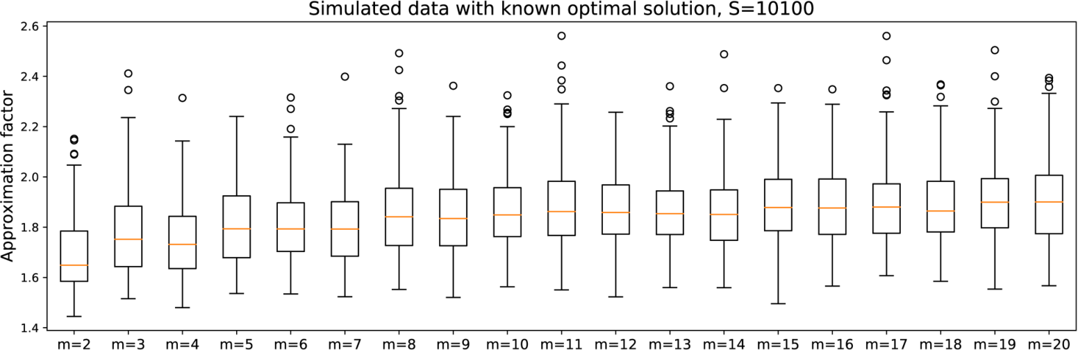
In the experiment of Figure 4, we once more study the approximation factor achieved by our algorithm. We place 100 optimal centers at , , and sample points around them such that for every center the farthest point in its cluster is at distance 0.5 from the center (Euclidean distance). One such a point set can be seen in the left plot of Figure 4. We randomly assign every point and center to one of groups and set to the number of centers that have been assigned to group . We let . For , the right part of Figure 4 shows boxplots of the approximation factors for our algorithm. Similarly as before, the approximation factor achieved by our algorithm is never larger than 2.6. Most interestingly, the approximation factor increases very moderately with .


5.3 Comparison with Baseline Approaches
We compare our algorithm in terms of the cost of an approximate solution to two linear-time baseline heuristics for the fair -center problem (2). The first one, referred to as Heuristic A, runs Algorithm 1 on each group separately (with and for group ) and outputs the union of the centers obtained for the groups. The second one, Heuristic B, greedily chooses centers similarly to Algorithm 1, but only from those groups for which we have not reached the requested number of centers yet. It is easy to see that the approximation factor achieved by these heuristics can be arbitrarily large on some worst-case instances.


Figure 6 shows boxplots of the costs of the approximate solutions returned by our algorithm and the two heuristics for three data sets: the data set in the left plot consists of vertices of a random graph constructed similarly as in the experiments of Figure 3. We set , , , and . The data set in the middle and in the right plot consists of the first 25000 records of the Adult data set (Dua & Graff 2019). We only use its six numerical features (e.g., age, hours worked per week), normalized to zero mean and unit variance, for representing records and use the -distance as metric . For the experiment shown in the middle plot, we split the data set into two groups according to the sensitive feature gender (#Female=8291, #Male=16709) and set . For the experiment shown in the right plot, we split the data set into five groups according to the feature race (#White=21391, #Asian-Pac-Islander=775, #Amer-Indian-Eskimo=241, #Other=214, #Black=2379) and set , . In Figure 10 in Appendix B we present results for other choices of . We always let be a randomly chosen subset of size . The two heuristics perform surprisingly well. Although coming without any worst-case guarantees, the cost of their solutions is comparable to the cost of the output of our algorithm.
5.4 Comparison with Unfair Algorithm 1
We compare the cost of the solution produced by our algorithm to the cost of the (potentially) unfair solution provided by Algorithm 1. Of course, we expect the latter to be lower. We consider the case , , and also examine how balanced the numbers of centers from a group in the output of Algorithm 1 are. Figure 5 shows the results, where the data sets and settings equal the ones in the experiments of Figure 6. Similar experiments with different settings are provided in Figure 12 in Appendix B. Remarkably, the costs of the solutions produced by our algorithm and Algorithm 1 have the same order of magnitude in all experiments, showing that the price of fairness is small. On the other hand, the output of Algorithm 1 can be highly unfair.
6 Discussion
In this work, we considered -center clustering under a fairness constraint that is motivated by the application of centroid-based clustering for data summarization. We presented a simple approximation algorithm with running time only linear in the size of the data set and the number of centers and proved our algorithm to be a 5-approximation algorithm when consists of two groups. For more than two groups, we proved an upper bound on the approximation factor that increases exponentially with the number of groups. We do not know whether this exponential dependence is necessary or whether our analysis is loose—in our extensive numerical simulations we never observed a large approximation factor. Besides answering this question, in future work it would be interesting to extend our results to -medoid clustering or to characterize properties of data sets that guarantee that fast algorithms find an optimal fair clustering.
Acknowledgements
This research is supported by a Rutgers Research Council Grant and a Center for Discrete Mathematics and Theoretical Computer Science (DIMACS) postdoctoral fellowship.
References
- Aggarwal et al. (2010) Aggarwal, G., Panigrahy, R., Feder, T., Thomas, D., Kenthapadi, K., Khuller, S., and Zhu, A. Achieving anonymity via clustering. ACM Transactions on Algorithms, 6(3):49:1–49:19, 2010.
- Angwin et al. (2016) Angwin, J., Larson, J., Mattu, S., and Kirchner, L. Propublica—machine bias, 2016. https://www.propublica.org/article/machine-bias-risk-assessments-in-criminal-sentencing.
- Arya et al. (2004) Arya, V., Garg, N., Khandekar, R., Meyerson, A., Munagala, K., and Pandit, V. Local search heuristics for -median and facility location problems. SIAM Journal on Computing, 33(3):544–562, 2004.
- Bolukbasi et al. (2016) Bolukbasi, T., Chang, K.-W., Zou, J., Saligrama, V., and Kalai, A. Man is to computer programmer as woman is to homemaker? Debiasing word embeddings. In Neural Information Processing Systems (NIPS), 2016.
- Buolamwini & Gebru (2017) Buolamwini, J. and Gebru, T. Gender shades: Intersectional accuracy disparities in commercial gender classification. In Conference on Fairness, Accountability, and Transparency (ACM FAT), 2017.
- Celis et al. (2018a) Celis, L. E., Huang, L., and Vishnoi, N. K. Multiwinner voting with fairness constraints. In International Joint Conference on Artificial Intelligence (IJCAI), 2018a.
- Celis et al. (2018b) Celis, L. E., Keswani, V., Straszak, D., Deshpande, A., Kathuria, T., and Vishnoi, N. K. Fair and diverse DPP-based data summarization. In International Conference on Machine Learning (ICML), 2018b. Code available on https://github.com/DamianStraszak/FairDiverseDPPSampling.
- Celis et al. (2018c) Celis, L. E., Straszak, D., and Vishnoi, N. K. Ranking with fairness constraints. In International Colloquium on Automata, Languages and Programming (ICALP), 2018c.
- Chakrabarty & Negahbani (2018) Chakrabarty, D. and Negahbani, M. Generalized center problems with outliers. In International Colloquium on Automata, Languages, and Programming (ICALP), 2018.
- Charikar et al. (2002) Charikar, M., Guha, S., Tardos, E., and Shmoys, D. B. A constant-factor approximation algorithm for the -median problem. Journal of Computer and System Sciences, 65(1):129–149, 2002.
- Chen et al. (2016) Chen, D. Z., Li, J., Liang, H., and Wang, H. Matroid and knapsack center problems. Algorithmica, 75:27–52, 2016.
- Chierichetti et al. (2017) Chierichetti, F., Kumar, R., Lattanzi, S., and Vassilvitskii, S. Fair clustering through fairlets. In Neural Information Processing Systems (NIPS), 2017.
- Cook et al. (1998) Cook, W. J., Cunningham, W. H., Pulleyblank, W. R., and Schrijver, A. Combinatorial Optimization. Wiley, 1998.
- Cormen et al. (2009) Cormen, T. H., Leiserson, C. E., Rivest, R. L., and Stein, C. Introduction to Algorithms. MIT Press, 3rd edition, 2009.
- Cygan et al. (2012) Cygan, M., Hajiaghayi, M., and Khuller, S. LP rounding for -centers with non-uniform hard capacities. In Symposium on Foundations of Computer Science (FOCS), 2012.
- Donini et al. (2018) Donini, M., Oneto, L., Ben-David, S., Shawe-Taylor, J., and Pontil, M. Empirical risk minimization under fairness constraints. In Neural Information Processing Systems (NeurIPS), 2018.
- Dua & Graff (2019) Dua, D. and Graff, C. UCI machine learning repository, 2019. https://archive.ics.uci.edu/ml/datasets/adult.
- Feldman et al. (2015) Feldman, M., Friedler, S. A., Moeller, J., Scheidegger, C., and Venkatasubramanian, S. Certifying and removing disparate impact. In ACM International Conference on Knowledge Discovery and Data Mining (KDD), 2015.
- Ferone et al. (2017) Ferone, D., Festa, P., Napoletano, A., and Resende, M. G. C. A new local search for the -center problem based on the critical vertex concept. In International Conference on Learning and Intelligent Optimization (LION), 2017.
- Girdhar & Dudek (2012) Girdhar, Y. and Dudek, G. Efficient on-line data summarization using extremum summaries. In International Conference on Robotics and Automation (ICRA), 2012.
- Gonzalez (1985) Gonzalez, T. F. Clustering to minimize the maximum intercluster distance. Theoretical Computer Science, 38:293–306, 1985.
- Hajiaghayi et al. (2010) Hajiaghayi, M., Khandekar, R., and Kortsarz, G. The red-blue median problem and its generalization. In European Symposium on Algorithms (ESA), 2010.
- Har-Peled (2011) Har-Peled, S. Geometric approximation algorithms. American Mathematical Society, 2011.
- Hardt et al. (2016) Hardt, M., Price, E., and Srebro, N. Equality of opportunity in supervised learning. In Neural Information Processing Systems (NIPS), 2016.
- Hastie et al. (2009) Hastie, T., Tibshirani, R., and Friedman, J. The Elements of Statistical Learning — Data Mining, Inference, and Prediction. Springer, 2nd edition, 2009.
- Hesabi et al. (2015) Hesabi, Z. R., Tari, Z., Goscinski, A., Fahad, A., Khalil, I., and Queiroz, C. Data summarization techniques for big data—a survey. In Handbook on Data Centers, pp. 1109–1152. Springer, 2015.
- Hochbaum & Shmoys (1986) Hochbaum, D. S. and Shmoys, D. B. A unified approach to approximation algorithms for bottleneck problems. Journal of the ACM, 33(3):533–550, 1986.
- Kale (2018) Kale, S. Small space stream summary for matroid center. arXiv:1810.06267 [cs.DS], 2018.
- Kay et al. (2015) Kay, M., Matuszek, C., and Munson, S. A. Unequal representation and gender stereotypes in image search results for occupations. In Conference on Human Factors in Computing Systems (CHI), 2015.
- Kleindessner et al. (2019) Kleindessner, M., Samadi, S., Awasthi, P., and Morgenstern, J. Guarantees for spectral clustering with fairness constraints. In International Conference on Machine Learning (ICML), 2019.
- Krishnaswamy et al. (2011) Krishnaswamy, R., Kumar, A., Nagarajan, V., Sabharwal, Y., and Saha, B. The matroid median problem. In Symposium on Discrete Algorithms (SODA), 2011.
- Kulesza & Taskar (2012) Kulesza, A. and Taskar, B. Determinantal point processes for machine learning. Foundations and Trends in Machine Learning, 5:123–286, 2012.
- Li & Svensson (2013) Li, S. and Svensson, O. Approximating -median via pseudo-approximation. In Symposium on the Theory of Computing (STOC), 2013.
- Mladenović et al. (2003) Mladenović, N., Labbé, M., and Hansen, P. Solving the -center problem with tabu search and variable neighborhood search. Networks, 42(1):48–64, 2003.
- Moens et al. (1999) Moens, M.-F., Uyttendaele, C., and Dumortier, J. Abstracting of legal cases: The potential of clustering based on the selection of representative objects. Journal of the American Society for Information Science, 50(2):151–161, 1999.
- Rösner & Schmidt (2018) Rösner, C. and Schmidt, M. Privacy preserving clustering with constraints. In International Colloquium on Automata, Languages, and Programming (ICALP), 2018.
- Samadi et al. (2018) Samadi, S., Tantipongpipat, U., Morgenstern, J., Singh, M., and Vempala, S. The price of fair PCA: One extra dimension. In Neural Information Processing Systems (NeurIPS), 2018.
- Schmidt et al. (2018) Schmidt, M., Schwiegelshohn, C., and Sohler, C. Fair coresets and streaming algorithms for fair k-means clustering. arXiv:1812.10854 [cs.DS], 2018.
- Sweeney (2013) Sweeney, L. Discrimination in online ad delivery. Queue, 11(3):10–29, 2013.
- Vazirani (2001) Vazirani, V. Approximation Algorithms. Springer, 2001.
- Zafar et al. (2017) Zafar, M. B., Valera, I., Rodriguez, M. G., and Gummadi, K. P. Fairness constraints: Mechanisms for fair classification. In International Conference on Artificial Intelligence and Statistics (AISTATS), 2017.
Appendix
Appendix A Proofs
Proof of Lemma 1:
It is straightforward to see that Algorithm 1 can be implemented in time . We only need to show that it is a 2-approximation algorithm for (3).
If , there is nothing to show, so assume that . Let be the output of Algorithm 1 and be an optimal solution to (3) with objective value . Let be arbitrary. We need to show that for some . If , there is nothing to show. So assume . If
there exists with and we are done. Otherwise, let and hence . We distinguish two cases:
- •
with :
We have and hence .
- •
with :
There must be , where not both and can be in , and such that
Since and , it follows that .
Without loss of generality, assume that in the execution of Algorithm 1, has been added to the set of centers after has been added. In particular, we have and for some . Due to the greedy choice in Line 5 of the algorithm and since has not been chosen by the algorithm, we have
Proof of Theorem 1:
Again it is easy to see that Algorithm 2 can be implemented in time . We need to prove that it is a 5-approximation algorithm, but not a -approximation algorithm for any :
- 1.
Algorithm 2 is a 5-approximation algorithm:
Let be the optimal value of the fair problem (2) and be the optimal value of the unfair problem (3). Clearly, . Let with and be an optimal solution to the fair problem (2) with cost and be the centers returned by Algorithm 2. It is clear that Algorithm 2 returns many elements from and many elements from and hence with and . We need to show that
Let be the output of Algorithm 1 when called in Line 3 of Algorithm 2. Since Algorithm 1 is a 2-approximation algorithm for the unfair problem (3) according to Lemma 1, we have
(6) If Algorithm 2 returns in Line 6, that is , we are done. Otherwise assume, as in the algorithm, that . Let be a center of cluster that we replace with and let be an arbitrary element in . Because of (6), we have and , and hence due to the triangle inequality. Consequently, after the while-loop in Line 9, every is in distance of or smaller to the center of its cluster. In particular, we have
and if Algorithm 2 returns in Line 13, we are done. Otherwise, we still have after exchanging centers in the while-loop in Line 9. Let , that is the union of clusters with a center . Since there is no more center in that we can exchange for an element in , we have . Let be the union of clusters with a center and be the union of clusters with a center in . Then we have . We have and
(7) Hence we only need to show that for every . We split into two subsets , where
and . For every there is with and it follows from (7) and the triangle inequality that
(8) It remains to show that for every . For every there exists with . We can write (some of the sets in this union might be empty, but that does not matter). Note that for every we have
(9) due to the triangle inequality. It is
and when, in Line 15 of Algorithm 2, we run Algorithm 1 on with and initial centers , one of the following three cases has to happen (we denote the centers returned by Algorithm 1 by ):
- •
For every there exists such that . In this case it immediately follows from (9) that
- •
- •
In all cases we have
which completes the proof of the claim that Algorithm 2 is a 5-approximation algorithm.
- •
- 2.
Algorithm 2 is not a -approximation algorithm for any :
Figure 7: An example showing that Algorithm 2 is not a -approximation algorithm for any . Consider the example given by the weighted graph shown in Figure 7, where . We have with and . All distances are shortest-path-distances. Let , , and . We assume that Algorithm 1 in Line 3 of Algorithm 2 picks as first center. It then chooses as second center, as third center and as fourth center. Hence, and . The clusters corresponding to are , , and . Assume we replace with and with in Line 10 of Algorithm 2. Then it is still , and in Line 15 of Algorithm 2 we run Algorithm 1 on with and initially given centers . Algorithm 1 returns . Finally, assume that is chosen as arbitrary third center from in Line 16 of Algorithm 2. So the centers returned by Algorithm 2 are with a cost of (incurred for ). However, the optimal solution has cost only . Choosing sufficiently small shows that Algorithm 2 is not a -approximation algorithm for any .
Proof of Lemma 2:
We want to show three things:
- 1.
Algorithm 3 is well-defined:
If the condition of the while-loop in Line 7 is true, there exists a shortest path with , that connects to in . Since is a shortest path, all are distinct. By the definition of , for every there exists with center and . Hence, the for-loop in Line 8 is well defined.
- 2.
Algorithm 3 terminates:
Let, at the beginning of the execution of Algorithm 3 in Line 3, , and . For , never changes during the execution of the algorithm. For , never increases during the execution of the algorithm and decreases at most until it equals . For , never decreases during the execution of the algorithm and increases at most until it equals . In every iteration of the while-loop, there is for which increases by one. It follows that the number of iterations of the while-loop is upper-bounded by .
- 3.
Algorithm 3 exchanges centers in such a way that the set that it returns satisfies and properties (4) and (5):
Note that throughout the execution of Algorithm 3 we have for the current centers . If the condition of the if-statement in Line 13 is true, then and (4) and (5) are satisfied.
Assume that the condition of the if-statement in Line 13 is not true. Clearly, the set returned by Algorithm 3 satisfies (5). Since the condition of the if-statement in Line 13 is not true, there exist with and with . We have , but since the condition of the while-loop in Line 7 is not true, we cannot have . This shows that . We need to show that (4) holds. Let be a cluster with center for some and assume it contained an element with . But then we had a path from to in . If , this is an immediate contradiction to . If , since , there exists such that there is a path from to . But then there is also a path from to , which is a contradiction to .
Proof of Theorem 2:
For showing that Algorithm 4 is a -approximation algorithm let be the optimal value of problem (2) and be an optimal solution with cost . Let be the centers returned by Algorithm 4. A simple proof by induction over shows that actually comprises many elements from every group . We need to show that
| (10) |
Let be the total number of calls of Algorithm 4, that is we have one initial call and recursive calls. Since with each recursive call the number of groups is decreased by at least one, we have . For , let be the data set in the -th call of Algorithm 4. We additionally set . We have and , . For , let be the set of groups in returned by Algorithm 3 in Line 8 in the -th call of Algorithm 4. If in the -th call of Algorithm 4 the algorithm terminates from Line 10 (note that in this case we must have ), we also let be the set of groups in returned by Algorithm 3 in the -th call. Otherwise we leave undefined. Setting , we have for all such that is defined. For , let be the set of centers returned by Algorithm 3 in Line 8 in the -th call of Algorithm 4 that belong to a group not in (in Algorithm 4, the set of these centers is denoted by ). We analogously define if in the -th call of Algorithm 4 the algorithm terminates from Line 10. Note that the centers in are comprised in the final output of Algorithm 4, that is for or . As always, denotes the set of centers that are given initially (for the initial call of Algorithm 4). Note that in the -th call of Algorithm 4 the set of initially given centers is .
We first prove by induction that for all such that is defined, that is or , we have
| (11) |
Base case : In the first call of Algorithm 4, Algorithm 1, when called in Line 3 of Algorithm 4, returns an approximate solution to the unfair problem (3). Let be the optimal cost of (3). Since Algorithm 1 is a 2-approximation algorithm for (3) according to Lemma 1, after Line 3 of Algorithm 4 we have
Let be a center and be two points in its cluster. It follows from the triangle inequality that . Hence, after running Algorithm 3 in Line 8 of Algorithm 4 and exchanging some of the centers in , we have for every , where denotes the center of its cluster. In particular,
for all for which its center is in or in a group not in , that is for .
Inductive step : Recall property (4) of a set returned by Algorithm 3. Consequently, only comprises items in a group in and, additionally, the given centers .
We split into two subsets , where
and . For every there exists
with . It follows from the inductive hypothesis that there exists with and consequently
Hence,
| (12) |
For every there exists with . Let with , where is the number of requested centers from group . We can write
where some of the sets in this union might be empty, but that does not matter. Note that for every we have
| (13) |
due to the triangle inequality. It is
and when, in Line 3 of Algorithm 4, we run Algorithm 1 on with and initial centers , one of the following three cases has to happen (we denote the centers returned by Algorithm 1 in this -th call of Algorithm 4 by and assume that for Algorithm 1 has chosen before ):
- •
For every there exists such that . In this case it immediately follows that
and using (12) we obtain
- •
- •
In any case, we have
| (14) |
Similarly to the base case, it follows from the triangle inequality that after running Algorithm 3 in Line 8 of Algorithm 4 and exchanging some of the centers in , we have
for every , where denotes the center of its cluster. In particular, we have
and this completes the proof of (11).
If in the -th call of Algorithm 4 the algorithm terminates from Line 10, it follows from (11) that
| (15) |
In this case, since , we have
and (15) implies (10). If in the -th call of Algorithm 4 the algorithm does not terminate from Line 10, it must terminate from Line 5. It follows from (11) that
| (16) |
In the same way as we have shown (14) in the inductive step in the proof of (11), we can show that
| (17) |
where is the set of centers returned by Algorithm 1 in the -th call of Algorithm 4. Since is contained in the output of Algorithm 4, (17) together with (16) implies (10).
Since running Algorithm 4 involves at most (recursive) calls of the algorithm and the running time of each of these calls is dominated by the running times of Algorithm 1 and Algorithm 3, it follows that the running time of Algorithm 4 is .
Proof of Lemma 3:
Consider the example given by the weighted graph shown in Figure 8, where . We have with , and . All distances are shortest-path-distances. Let , , and . We assume that Algorithm 1 in Line 3 of Algorithm 4 picks as first center. It then chooses as second center, as third center, as fourth center, as fifth center and as sixth center. Hence, and the corresponding clusters are , , , , and . When running Algorithm 3 in Line 8 of Algorithm 4, it replaces with one of , or and it replaces with one of , or . Assume that it replaces with and with . Algorithm 3 then returns and when recursively calling Algorithm 4 in Line 12, we have and . In the recursive call, the given centers are and Algorithm 1 chooses and . The corresponding clusters are , , and . When running Algorithm 3 with clusters and , it replaces with either or and returns , that is afterwards we are done. Assume Algorithm 3 replaces with . Then the centers returned by Algorithm 4 are and two arbitrary elements from , which we assume to be and . These centers have a cost of (incurred for ). However, an optimal solution such as has cost only . Choosing sufficiently small shows that Algorithm 4 is not a -approximation algorithm for any .
Appendix B Further Experiments
In Figure 9 we show the costs of the approximate solutions produced by our algorithm (Alg. 4) and the algorithm by Chen et al. 2016 (M.C.) in the run-time experiment shown in the right part of Figure 3. In Figure 10, Figure 11 and Figure 12 we provide similar experiments as shown in Figure 6, Figure 2 and Figure 5, respectively.


| Algorithm 1 | Our Algorithm | Celis et al. 2018b |
 |
 |
 |


