跳到论文正文
W Papers独立论文阅读器 arXiv:1901.08571 论文正文 计算阅读时间 · 0%
引用这篇论文根据当前论文元数据生成,正式投稿前建议核对。


License: arXiv.org perpetual non-exclusive license
arXiv:1901.08571v3 [math.ST] 11 Aug 2023

Kexuan Li, Ruiqi Liu, GanggangXu and Zuofeng Shang

Nonparametric Inference under B-bits Quantization

Kexuan Li kexuan.li.77@gmail.com Affiliation: Global Analytics and Data Sciences Affiliation: Biogen Inc Affiliation: Cambridge, MA 02142 USA    Ruiqi Liu ruiqliu@ttu.edu Affiliation: Department of Mathematics and Statistics Affiliation: Texas Tech University Affiliation: Lubbock, TX 79409, USA    Ganggang Xu gangxu@bus.miami.edu Affiliation: Department of Management Science Affiliation: University of Miami Affiliation: Coral Gables, FL 33146, USA    Zuofeng Shang zshang@njit.edu Affiliation: Department of Mathematical Sciences Affiliation: New Jersey Institute of Technology Affiliation: Newark, NJ 07102, USA
Abstract

Statistical inference based on lossy or incomplete samples is often needed in research areas such as signal/image processing, medical image storage, remote sensing, signal transmission. In this paper, we propose a nonparametric testing procedure based on samples quantized to BB bits through a computationally efficient algorithm. Under mild technical conditions, we establish the asymptotic properties of the proposed test statistic and investigate how the testing power changes as BB increases. In particular, we show that if BB exceeds a certain threshold, the proposed nonparametric testing procedure achieves the classical minimax rate of testing (Shang and Cheng 2015) for spline models. We further extend our theoretical investigations to a nonparametric linearity test and an adaptive nonparametric test, expanding the applicability of the proposed methods. Extensive simulation studies together with a real-data analysis are used to demonstrate the validity and effectiveness of the proposed tests.

††heading: 1 2000 1-68 4/00 10/00 meila00a††shortheadings: Nonparametric Inference under B-bits Quantization / Li, Liu, Xu and Shang††firstpage: 1††editor: Rina Barber
keywords
B-bits Quantization, Minimax Rates of Testing, Nonparametric Inference, Smoothing Splines

1 Introduction

Lossy or incomplete data are commonly encountered in research areas such as machine learning, information theory, and signal processing. To store and process signals in digital devices, quantization is a popular procedure that maps the original measurements from a large (often uncountably infinite) set to a set of possible values. The resulting values are referred to as the quantized samples. With the increasing availability of data, it is of great interest to quantify how the data analysis can be affected when the data are quantized due to storage or communication budget constraint, and how to design quantization schemes to minimize the efficiency loss. Statistical inference based on quantized samples is challenging because, in addition to the measurement errors, one also needs to account for the information loss due to the quantization errors. In particular, commonly used standard statistical procedures may not be valid when applied to quantized samples if the quantization errors are ignored.

The research on lossy data has attracted increasing attention recently. The first line of works focuses on bb-bit compressive sensing, which aims at reconstructing a sparse signal from a sequence of bb-bit quantized outcomes. A 11-bit compressive sensing model was proposed by Boufounos and Baraniuk 2008, and several efficient and provable algorithms have been developed; see, e.g., Gupta et al. 2010; Gopi et al. 2013; Plan and Vershynin 2013; Zhang et al. 2014; Zhu and Gu 2015. A signal recovery algorithm was proposed in Slawski and Li 2015, which extended the 11-bit compressive sensing model to a bb-bit compressive sensing model. The second line of research related to the lossy data is to develop statistical methods based on quantized observations. For example, Lee and Vardeman 2001 studied the interval estimation of a normal mean process from rounded data, which was further extended to more general likelihood-based statistical estimation problems (Vardeman and Lee 2005) and nonparametric regression problems (Benhenni and Rachdi 2006). Recently, an increasing number of works aim to quantify the impact of quantization on the statistical properties of the resulting estimators. For example, Zhang et al. 2013 established lower bounds on the minimax risks for distributed estimation of parametric models under a communication budget constraint. Suresh et al. 2017 proposed communication efficient algorithms for distributed mean estimation without probabilistic assumptions on the data. A version of Pinsker’s theorem under some storage or communication constraints was developed in Zhu and Lafferty 2014, and it was further applied to analyze the convergence rate of nonparametric estimation with a limited bits budget by Zhu and Lafferty 2017. More recently, a series of works have emerged in investigating the high-dimensional and/or nonparametric regression model estimation in the distributed learning framework with bits constraints, e.g., see Zhu and Lafferty 2018; Han et al. 2018; Szabo and van Zanten 2020; Cai and Wei 2021.

Despite the abundant existing literature on statistical modeling of quantized data, research focusing on the nonparametric inference based on quantized data is still lacking. This paper aims to fill this gap by proposing a new quantization scheme with a BB-bits storage or communication budget such that nonparametric estimation and testing based on quantized samples are still valid. Specifically, we consider the following regression model

yi=g0(i/n)+σϵi,i=1,…,n,y_{i}=g_{0}(i/n)+\sigma\epsilon_{i},\,\,i=1,\ldots,n, (1)

where g0​(⋅)g_{0}(\cdot) is a smooth function, ϵi\epsilon_{i}’s are iid zero-mean errors with an unit variance, and σ>0\sigma>0 is an unknown constant. The goal is to (a) estimate g0​(⋅)g_{0}(\cdot), and (b) test the following hypothesis

H0: g0​(x)=g∗​(x) for all x∈[0,1],\displaystyle H_{0}:\,\,\textrm{ $g_{0}(x)=g_{*}(x)$ for all $x\in[0,1]$}, (2)

where g∗​(⋅)g_{*}(\cdot) is a pre-specified deterministic function.

The above model has been extensively studied in the literature, see, e.g., Shang and Cheng 2017, and is closely related to the well-known Gaussian sequence model and Gaussian white noise model (Tsybakov 2008). However, unlike existing literature, we consider the case in which the original data, denoted by y1,⋯,yny_{1},\cdots,y_{n}, are generated in machine M, and are quantized as soon as they are generated. The quantized data are then stored in a machine M or transmitted to another machine M∗ for future statistical inferences. We assume that only BB-bits budget are available for data storage or communication, rendering the necessity for data quantization that may invalidate existing estimation and inference methods. Such a research problem is important for applications where data generation and analysis are carried out at different locations. For example, testing H0:g0​(x)=0H_{0}:g_{0}(x)=0 reveals whether the transmitted quantized signals through satellite are pure noises. If g∗​(⋅)g_{*}(\cdot) is the signal-process from a normally functioning machine, testing (2) using only quantized samples enables us to remotely monitor whether the machine is working properly in real-time.

To meet the BB-bits requirement, we propose a two-stage quantization procedure: in the first stage we quantize an individual yiy_{i} as Q⁡(yi)Q(y_{i}) with Q⁡(⋅)Q(\cdot) being a quantizer, and in the second stage we overwrite these quantized observations by their local averages. See Figure 1 and Algorithm 1 for details. As a result, we obtain a quantized sample of size cc for some c<nc<n to be stored or transmitted. We demonstrate that with a carefully chosen cc and a well-designed quantizer, the proposed nonparametric estimation and testing procedures are asymptotically valid and efficient even based only on the quantized data.

Our contributions can be summarized as follows. Firstly, we propose a computationally efficient data quantization algorithm to reduce the size of the raw data to meet the BB-bits constraint, and at the same time reduce the computational complexity from O⁡(n3)O(n^{3}) to O⁡(c3)O(c^{3}). Secondly, we establish sufficient conditions on the bits constraint, i.e., BB, that warrants the minimax convergence rate for the resulting spline estimators and the minimax rates of testing for the proposed testing procedure. In particular, our results show how the asymptotic power of the proposed testing procedure changes as the bits constraint BB increases. Thirdly, we further extend our theoretical investigations to (a) a nonparametric linearity test of the underlying function; (b) an adaptive nonparametric test when the smoothness of the underlying function is unknown. To the best of our knowledge, our work is the first to provide a theoretical investigation on nonparametric inference based on quantized samples.

The rest of the paper is organized as follows. Section 2 describes the general methodologies we proposed for data quantization, nonparametric estimation, and nonparametric testing using splines. In Section 3, we investigate the theoretical properties of the spline estimator and the nonparametric test statistic based on quantized samples. In Section 4, we study asymptotic properties of the nonparametric linearity test statistic and the adaptive nonparametric test statistic under B-bits constraint. Section 5 gives several simulation studies to evaluate finite sample performances of the proposed methods and Section 6 illustrates an application of the proposed methods to the Combined Cycle Power Plant Data.

Notation: Let ∥⋅∥\|\cdot\| represent the L2L^{2}-norm, i.e., ‖f‖2=∫01f2​(t)​𝑑t\|f\|^{2}=\int_{0}^{1}f^{2}(t)dt, and define ∥⋅∥2\|\cdot\|_{2} as the Euclidean Norm of vectors. Let ∥⋅∥sup\|\cdot\|_{\sup} denote the supreme norm of a function, i.e., ‖f‖sup=supt∈[0,1]|f⁡(t)|\|f\|_{\sup}=\sup_{t\in[0,1]}|f(t)|. For two positive sequences ana_{n} and bnb_{n}, we denote an≳bna_{n}\gtrsim b_{n} (an≲bna_{n}\lesssim b_{n}) if there exists a constant C>0C>0 such that an≥C​bna_{n}\geq Cb_{n} (an≤C​bna_{n}\leq Cb_{n}) for all n≥1n\geq 1; denote an≍bna_{n}\asymp b_{n} if an≳bna_{n}\gtrsim b_{n} and an≲bna_{n}\lesssim b_{n}; denote an≪bna_{n}\ll b_{n} if an/bn→0a_{n}/b_{n}\to 0 as n→∞n\to\infty and an≫bna_{n}\gg b_{n} if an/bn→∞a_{n}/b_{n}\to\infty as n→∞n\to\infty.

2 Methodology

In this section, we first review some background of the classical smoothing spline regression and then give details on the proposed quantization scheme, nonparametric estimation and testing procedures.

2.1 Review of Classical Smoothing Spline Regression

Throughout this paper, we assume that the underlying true function g0​(⋅)g_{0}(\cdot) belongs to the mm-order (m≥1m\geq 1) periodic Sobolev space on 𝕀:=[0,1]\mathbb{I}:=[0,1] defined as

Sm​(𝕀)={∑ν=1∞βν​φν​(⋅):∑ν=1∞βν2​γν<∞},S^{m}(\mathbb{I})=\left\{\sum_{\nu=1}^{\infty}\beta_{\nu}\varphi_{\nu}(\cdot):\sum_{\nu=1}^{\infty}\beta_{\nu}^{2}\gamma_{\nu}<\infty\right\},

where φ2​k−1​(x)=2​cos⁡(2​π​k​x),φ2​k​(x)=2​sin⁡(2​π​k​x)\varphi_{2k-1}(x)=\sqrt{2}\cos(2\pi kx),\,\,\,\,\varphi_{2k}(x)=\sqrt{2}\sin(2\pi kx) are the trigonometric basis functions, and γ2​k−1=γ2​k=(2​π​k)2​m\gamma_{2k-1}=\gamma_{2k}=(2\pi k)^{2m} for x∈𝕀x\in\mathbb{I} and k≥1k\geq 1. It follows from Wahba 1990 and Gu 2013 that Sm​(𝕀)S^{m}(\mathbb{I}) is a reproducing kernel Hilbert space (RKHS) endowed with an inner product J⁡(f,g)=∫01f(m)​(x)​g(m)​(x)​𝑑xJ(f,g)=\int_{0}^{1}f^{(m)}(x)g^{(m)}(x)dx and a reproducing kernel

K⁡(x,y)=(−1)m−1(2​m)!​B2​m​(|x−y|),K(x,y)=\frac{(-1)^{m-1}}{(2m)!}B_{2m}(|x-y|),

where B2​mB_{2m} is the Bernoulli polynomial of order 2​m2m.

Based on the above assumptions on g0​(⋅)g_{0}(\cdot), the classic smoothing spline (ss) estimator of g0​(⋅)g_{0}(\cdot) is obtained through the following optimization problem:

g^ss\displaystyle\widehat{g}^{\textrm{ss}} ≡arg​ming∈Sm⁡1n​∑i=1n(yi−g⁡(i/n))2+λ​∫01[g(m)​(x)]2​dx.\displaystyle\equiv\argmin_{g\in S^{m}}\frac{1}{n}\sum_{i=1}^{n}(y_{i}-g(i/n))^{2}+\lambda\int_{0}^{1}[g^{(m)}(x)]^{2}dx. (3)

For x∈𝕀x\in\mathbb{I}, we can define a function Kx​(⋅)=K⁡(x,⋅)K_{x}(\cdot)=K(x,\cdot), which belongs to Sm​(𝕀)S^{m}(\mathbb{I}). By the representer Theorem (Gu 2013), the solution to (3) has the following closed-form

g^ss=∑i=1nθi​Ki/n,\widehat{g}^{\textrm{ss}}=\sum_{i=1}^{n}\theta_{i}K_{i/n}, (4)

where θ=(θ1,…,θn)T=n−1​(Σn+λ​In)−1​y\theta=(\theta_{1},\ldots,\theta_{n})^{T}=n^{-1}(\Sigma_{n}+\lambda I_{n})^{-1}y with Σn=[K⁡(i/n,i′/n)/n]1≤i,i′≤n∈ℝn×n\Sigma_{n}=[K(i/n,i^{\prime}/n)/n]_{1\leq i,i^{\prime}\leq n}\in\mathbb{R}^{n\times n}, y=(y1,…,yn)T∈ℝny=(y_{1},\ldots,y_{n})^{T}\in\mathbb{R}^{n} and InI_{n} being the n×nn\times n identify matrix.

To conduct hypothesis test for (2), a straightforward idea is to construct a testing statistic based on the distance between g^ss​(⋅)\widehat{g}^{\textrm{ss}}(\cdot) and g∗​(⋅)g_{*}(\cdot). Specifically, we use the L2L_{2} norm distance defined as

Tss=‖g^s​s−g∗‖2.\displaystyle T^{\textrm{ss}}=\|\widehat{g}^{ss}-g_{*}\|^{2}.

With an appropriate normalization, it can be shown that TssT^{\textrm{ss}} is asymptotically normally distributed (Shang and Cheng 2017; Yang et al. 2020; Liu et al. 2021).

2.2 Two-Stage Quantization

The original observations yiy_{i}’s in (1) are real-valued random variables, each of which literally requires an infinite amount of bits to store or transmit. When there are only BB available bits, the original observations yiy_{i}’s may not be directly accessible for estimation or testing, and hence, the classical smoothing spline estimator given in (4) is not applicable. This section aims to introduce a two-stage quantization scheme to transform yiy_{i}’s into the ones whose storage or transmission meets the BB-bits constraint. The resulting samples will be further used for optimal inferential purposes in the subsequent sections. The two-stage quantization process is demonstrated in the following Figure 1.

Refer to caption
Figure 1: Two-stage quantization process.

The first-stage quantization is to quantize the data yiy_{i}’s as soon as they are generated with at most kk distinct values. For convenience, we use a uniform quantization scheme as follows. We first choose an interval [t1,tk−1][t_{1},t_{k-1}] and choose t2<…<tk−2t_{2}<\ldots<t_{k-2} as the equally spaced grid points within [t1,tk−1][t_{1},t_{k-1}]. Denote t=(t1,…,tk−1)T∈ℝk−1t=(t_{1},\ldots,t_{k-1})^{T}\in\mathbb{R}^{k-1} and the sub-interval length Ck​(t):=(tk−1−t1)/(k−2)C_{k}(t):=(t_{k-1}-t_{1})/(k-2). For ease of presentation, we assume that l1=t1/Ck​(t)l_{1}=t_{1}/C_{k}(t) is an integer. Define a quantizer Q⁡(⋅)Q(\cdot) as follows:

First-stage quantization:   Q(y)=∑j=1kμjI[y∈Rj(t)], with μj=(l1+j−1)Ck(t),\displaystyle Q(y)=\sum_{j=1}^{k}\mu_{j}I[y\in R_{j}(t)],\text{ with }\mu_{j}=(l_{1}+j-1)C_{k}(t), (5)
for any ​y∈ℝ,\displaystyle\text{ for any }y\in\mathbb{R},

where μ=(μ1,…,μk)T∈ℝk\mu=(\mu_{1},\ldots,\mu_{k})^{T}\in\mathbb{R}^{k} consists of the quantized values and R1(t)=(−∞,t1],R2(t)=(t1,t2],…,Rk−1(t)=(tk−2,tk−1]R_{1}(t)=(-\infty,t_{1}],R_{2}(t)=(t_{1},t_{2}],\ldots,R_{k-1}(t)=(t_{k-2},t_{k-1}], Rk​(t)=(tk−1,∞)R_{k}(t)=(t_{k-1},\infty) are the corresponding quantized intervals. Clearly, the Rj​(t)R_{j}(t)’s form a partition of the real line with assigned marks μj\mu_{j}’s and QQ maps each y∈ℝy\in\mathbb{R} to one of the kk marks. Applying QQ to yiy_{i}’s, we generate nn quantized samples Q⁡(y1),⋯,Q⁡(yn)Q({y}_{1}),\cdots,Q({y}_{n}), each of which takes at most kk distinct values. Storage or transmission of Q⁡(yi)Q(y_{i})’s thus requires n​log2​kn\log_{2}{k} bits which might still go beyond the BB-bits budget when B=o⁡(n)B=o(n). For this reason, we propose the following second-stage quantization to further reduce the storage or transmission bits through locally averaging the Q⁡(yi)Q(y_{i})’s.

The second-stage quantization is to further reduce the number of storage or transmission bits via local average. Specifically, we divide the interval 𝕀=[0,1]\mathbb{I}=[0,1] into cc equally-spaced sub-intervals for some c≤B/⌈log2⁡(k+2)⌉c\leq B/\lceil\log_{2}(k+2)\rceil. For simplicity, we assume that n~≔n/c\widetilde{n}\coloneqq n/c is an integer and each sub-interval contains n~\widetilde{n} observations. The quantized data from the first-stage quantization, i.e., Q⁡(yi)Q(y_{i})’s, are further quantized as zi=l~i​Ck​(t)z_{i}=\widetilde{l}_{i}C_{k}(t) such that

Second-stage quantization:|zi−1n~∑j=(i−1)​n~+1i​n~Q(yj)|≤Ck(t), for i=1,…,c.\textrm{Second-stage quantization:}\,\,\,\,\left|z_{i}-\frac{1}{\widetilde{n}}\sum_{j=(i-1)\widetilde{n}+1}^{i\widetilde{n}}Q(y_{j})\right|\leq C_{k}(t),\,\,\textrm{ for $i=1,\ldots,c$.} (6)

Details of the two-stage quantization algorithm are provided in the following Algorithm 1.

Initialization: set l~1=⋯=l~c=0\widetilde{l}_{1}=\cdots=\widetilde{l}_{c}=0;
Input: Data y1,⋯,yny_{1},\cdots,y_{n} that generated sequentially;
while 1≤i≤c1\leq i\leq c do
  1. Set tmp=0{\rm tmp}=0;

  2. while (i−1)​n~+1≤j≤i​n~(i-1)\widetilde{n}+1\leq j\leq i\widetilde{n} do

    1. (a)

      First-stage quantization (quantize on the spot): Q⁡(yj)=lj​Ck​(t)Q(y_{j})=l_{j}C_{k}(t);

    2. (b)

      Second-stage quantization (averaging):

      1. i.

        update l~i=l~i+Integer Part of ​lj/n~\widetilde{l}_{i}=\widetilde{l}_{i}+\text{Integer Part of }l_{j}/\widetilde{n};

      2. ii.

        if tmp+sign​(lj)​(|lj|​ mod ​n~)≥n~{\rm tmp}+\text{sign}(l_{j})(|l_{j}|\text{ mod }\widetilde{n})\geq\widetilde{n} then
          update {l~i:=l~i+1tmp:=tmp+sign​(lj)​(|lj|​ mod ​n~)−n~;\begin{cases}\widetilde{l}_{i}:=\widetilde{l}_{i}+1\\ {\rm tmp}:={\rm tmp}+\text{sign}(l_{j})(|l_{j}|\text{ mod }\widetilde{n})-\widetilde{n};\end{cases}

      3. else if tmp+sign​(lj)​(|lj|​ mod ​n~)≤−n~{\rm tmp}+\text{sign}(l_{j})(|l_{j}|\text{ mod }\widetilde{n})\leq-\widetilde{n} then
          update {l~i:=l~i−1tmp:=tmp+sign​(lj)​(|lj|​ mod ​n~)+n~;\begin{cases}\widetilde{l}_{i}:=\widetilde{l}_{i}-1\\ {\rm tmp}:={\rm tmp}+\text{sign}(l_{j})(|l_{j}|\text{ mod }\widetilde{n})+\widetilde{n};\end{cases}

      4. else
          update tmp:=tmp+sign​(lj)​(|lj|​ mod ​n~){\rm tmp}:={\rm tmp}+\text{sign}(l_{j})(|l_{j}|\text{ mod }\widetilde{n});
        end if

    end while

end while
Output: quantized data: z1=l~1​Ck​(t),⋯,zc=l~c​Ck​(t)z_{1}=\widetilde{l}_{1}C_{k}(t),\cdots,z_{c}=\widetilde{l}_{c}C_{k}(t).
Algorithm 1 Two-Stage Quantization

Based on the definition of the quantizer Q⁡(⋅)Q(\cdot) in (5), ziz_{i} in (6) must belong to the interval [μ1−Ck​(t),μk+Ck​(t)][\mu_{1}-C_{k}(t),\mu_{k}+C_{k}(t)] and must be of the form l​Ck​(t)lC_{k}(t) for some integer ll. Therefore, there are at most k+2k+2 distinct values of ziz_{i}’s, namely, l​Ck​(t)lC_{k}(t), for l=l1−1,l1,l1+1,⋯,(l1+k−1),l1+kl=l_{1}-1,l_{1},l_{1}+1,\cdots,(l_{1}+k-1),l_{1}+k. As a result, each ziz_{i} requires b=⌈log2⁡(k+2)⌉b=\lceil\log_{2}(k+2)\rceil bits to store or transmit, hence, the entire ziz_{i}’s require c⁡⌈log2⁡(k+2)⌉≤Bc\lceil\log_{2}(k+2)\rceil\leq B bits, where ⌈x⌉\lceil x\rceil is the smallest integer greater than xx. In the subsequent sections, we will show that, with c,kc,k being properly selected, optimal inferences based on ziz_{i}’s are possible even under B=o⁡(n)B=o(n), comparing to other regression literature which typically needs B≳nB\gtrsim n (see Slawski and Li 2018). For optimal inferences in non-regression settings such as Gaussian sequence model or Gaussian white-noise model, similar findings were made by Cai and Wei 2021.

2.3 BB-bits Nonparametric Spline Estimation

Given BB, let us choose k,ck,c such that c⁡⌈log2⁡(k+2)⌉=Bc\lceil\log_{2}(k+2)\rceil=B, i.e., our two-stage quantization maximizes the use of the available bits. Based on the quantized samples z1,…,zcz_{1},\ldots,z_{c} from Algorithm 1, a BB-bits constrained spline estimator is proposed as follows

g^μ,t,cB\displaystyle\widehat{g}^{\textrm{B}}_{\mu,t,c} ≡arg​ming∈Sm​(𝕀)⁡1c​∑i=1c(zi−g⁡(i/c))2+λ​∫01[g(m)​(x)]2​dx.\displaystyle\equiv\argmin_{g\in S^{m}(\mathbb{I})}\frac{1}{c}\sum_{i=1}^{c}(z_{i}-g(i/c))^{2}+\lambda\int_{0}^{1}[g^{(m)}(x)]^{2}dx. (7)

Similar to (4), the resulting spline estimator g^μ,t,cB​(⋅)\widehat{g}^{\textrm{B}}_{\mu,t,c}(\cdot) has an explicit expression

g^μ,t,cB=∑i=1cθ^i​Ki/c,\widehat{g}^{\textrm{B}}_{\mu,t,c}=\sum_{i=1}^{c}\widehat{\theta}_{i}K_{i/c},

where (θ^1,…,θ^c)T=c−1​(Σc+λ​Ic)−1​z(\widehat{\theta}_{1},\ldots,\widehat{\theta}_{c})^{T}=c^{-1}(\Sigma_{c}+\lambda I_{c})^{-1}z with Σc=[K⁡(i/c,i′/c)/c]1≤i,i′≤c∈ℝc×c\Sigma_{c}=[K(i/c,i^{\prime}/c)/c]_{1\leq i,i^{\prime}\leq c}\in\mathbb{R}^{c\times c}, z=(z1,…,zc)T∈ℝcz=(z_{1},\ldots,z_{c})^{T}\in\mathbb{R}^{c}, and IcI_{c} being the c×cc\times c identity matrix.

Notice that the optimization of (7) only requires on cc quantized observations and the solution only involves computing the inverse of a c×cc\times c matrix Σc+λ​Ic\Sigma_{c}+\lambda I_{c}, which is much less computationally intensive compared to the classical smoothing spline estimator (4).

Finally, the selection of the tuning parameter λ\lambda is crucial, and can be obtained by minimizing the generalized cross validation (GCV) score as follows

λ^=arg​minλ>0⁡c∥[Ic−Σc(Σc+λIc)−1)]z∥22[c−trace​(Σc​(Σc+λ​Ic)−1)]2,\widehat{\lambda}=\argmin_{\lambda>0}\frac{c\|[I_{c}-\Sigma_{c}(\Sigma_{c}+\lambda I_{c})^{-1})]z\|_{2}^{2}}{[c-\textrm{trace}(\Sigma_{c}(\Sigma_{c}+\lambda I_{c})^{-1})]^{2}}, (8)

The GCV has been widely used in the literature and enjoys appealing theoretical properties in various settings, see, e.g., Wahba 1990; Xu and Huang 2012; Gu 2013; Xu et al. 2018; Xu et al. 2019.

2.4 BB-bits Nonparametric Testing

In this section, we propose a test statistic for the null hypothesis (2) based on the BB-bits spline estimator g^μ,t,cB​(⋅)\widehat{g}_{\mu,t,c}^{\textrm{B}}(\cdot). Without loss of generality, we assume g∗​(⋅)≡0g_{*}(\cdot)\equiv 0 in the null hypothesis (2). For a nonzero g∗​(⋅)g_{*}(\cdot), the observed response variables yiy_{i}’s from model (1) can be centered as yi∗=yi−g∗​(i/n)y_{i}^{*}=y_{i}-g_{*}(i/n), and the same testing procedure can be applied using yi∗y_{i}^{*}’s instead. To test H0:g0​(x)=0H_{0}:g_{0}(x)=0, we consider test statistic based on the L2L_{2} norm distance between g^μ,t,cB​(⋅)\widehat{g}_{\mu,t,c}^{\textrm{B}}(\cdot) and g∗​(⋅)≡0g_{*}(\cdot)\equiv 0 as following

Tμ,t,c=‖g^μ,t,cB‖2.T_{\mu,t,c}=\|\widehat{g}_{\mu,t,c}^{\textrm{B}}\|^{2}. (9)

Intuitively, a large value of Tμ,t,cT_{\mu,t,c} should lead to the rejection of H0H_{0}. In Theorem 3, we shall show that under H0H_{0} and mild conditions, it holds that

c​Tμ,t,c−trace​(A)​τk2sc​τk2​⟶𝑑​N​(0,1)​as n,c→∞,\frac{cT_{\mu,t,c}-\textrm{trace}(A){\tau}_{k}^{2}}{s_{c}{\tau}_{k}^{2}}\overset{d}{\longrightarrow}N(0,1)\,\,\textrm{as $n,c\rightarrow\infty$,}

where τk2=Var​(z1|H0)\tau_{k}^{2}=\textrm{Var}(z_{1}|H_{0}), A=(Σc+λ​Ic)−1​Ωc​(Σc+λ​Ic)−1A=(\Sigma_{c}+\lambda I_{c})^{-1}\Omega_{c}(\Sigma_{c}+\lambda I_{c})^{-1}, Ωc=[K⊗2​(i/c,i′/c)/c]1≤i,i′≤c\Omega_{c}=[K^{\otimes 2}(i/c,i^{\prime}/c)/c]_{1\leq i,i^{\prime}\leq c} with K⊗2​(x,x′):=∫01K⁡(x,y)​K​(y,x′)​𝑑yK^{\otimes 2}(x,x^{\prime}):=\int_{0}^{1}K(x,y)K(y,x^{\prime})dy and sc2=2​∑1≤i≠i′≤cai,i′2s_{c}^{2}=2\sum_{1\leq i\neq i^{\prime}\leq c}a_{i,i^{\prime}}^{2} with ai,i′a_{i,i^{\prime}} being the (i,i′)(i,i^{\prime})th entry of AA. In practice, τk2\tau_{k}^{2} needs to be estimated based on the quantized data as well. We proposed the following estimator

τ^k2=τ~n22​n~​(n−1),\widehat{\tau}_{k}^{2}=\frac{\widetilde{\tau}_{n}^{2}}{2\widetilde{n}(n-1)},

where τ~n\widetilde{\tau}_{n} is given in the following Algorithm 2 through quantization. Intuitively, the above estimator is a re-scaled (by a factor of n~−1\widetilde{n}^{-1}) version of the quantized sample error variance 12​(n−1)​∑j=2n{Q⁡(yj)−Q⁡(yj−1)}2\frac{1}{2(n-1)}\sum_{j=2}^{n}\left\{Q(y_{j})-Q(y_{j-1})\right\}^{2}. It is straightforward to shown that τ^k2=τk2​[1+op​(1)]\widehat{\tau}_{k}^{2}=\tau_{k}^{2}[1+o_{p}(1)] under mild conditions, see Lemma 11 of Appendix C for details. Consequently, the decision rule for testing (2) at significance level α\alpha can be defined as follows

ϕc,k=I⁡(|c​Tμ,t,c−trace​(A)​τ^k2|≥z1−α/2​sc​τ^k2),\phi_{c,k}=I(|cT_{\mu,t,c}-\textrm{trace}(A)\widehat{\tau}_{k}^{2}|\geq z_{1-\alpha/2}s_{c}\widehat{\tau}_{k}^{2}), (10)

where z1−α/2z_{1-\alpha/2} is the (1−α/2)(1-\alpha/2)-percentile of the standard normal distribution. We reject the null hypothesis (2) if and only if ϕc,k=1\phi_{c,k}=1.

Initialization: set τ~n2=tmp=0\widetilde{\tau}_{n}^{2}={\rm tmp}=0;
Input: Data y1,⋯,yny_{1},\cdots,y_{n} that generated sequentially;
while 1≤j≤n1\leq j\leq n do
  1. 1.

    Quantize on the spot Q⁡(yj)Q(y_{j});

  2. 2.

    if j=1j=1 then update tmp:=Q⁡(y1){\rm tmp}:=Q(y_{1}); else

    1. (a)

      update τ~n2:=τ~n2+(Q⁡(yj)−tmp)2\widetilde{\tau}_{n}^{2}:={\widetilde{\tau}_{n}^{2}+(Q(y_{j})-{\rm tmp})^{2}};

    2. (b)

      update tmp:=Q⁡(yj){\rm tmp}:=Q(y_{j});

    end if

end while
Output: τ~n2\widetilde{\tau}_{n}^{2}.
Algorithm 2 Quantization Estimation of Variance

By the design of the quantizer Q⁡(⋅)Q(\cdot) in (5), we can see that there are at most k+1k+1 distinct possible values for each {Q⁡(yj+1)−Q⁡(yj)}2\left\{Q(y_{j+1})-Q(y_{j})\right\}^{2} ranging from 0​Ck​(t)20C_{k}(t)^{2} to k2​Ck​(t)2k^{2}C_{k}(t)^{2}, 1≤j≤n−11\leq j\leq n-1, yielding the range for τ~2\widetilde{\tau}^{2} as [0,(n−1)​k2​Ck​(t)2][0,(n-1)k^{2}C_{k}(t)^{2}]. Since τ~2\widetilde{\tau}^{2} can only take values as l​Ck​(t)2lC_{k}(t)^{2} for some integer ll, there are at most (n−1)​k2+1(n-1)k^{2}+1 distinct values for τ~2\widetilde{\tau}^{2}, which would cost ⌈log2⁡{(n−1)​k2+1}⌉\lceil\log_{2}\left\{(n-1)k^{2}+1\right\}\rceil bits to store or transmit. Compare to the bit costs for the two-stage quantization c⁡⌈log2⁡(k)⌉≈Bc\lceil\log_{2}(k)\rceil\approx B, the cost to store or transmit τ~2\widetilde{\tau}^{2} is negligible when c→∞c\to\infty, hence is ignored in the calculation of the total bit costs for ease of presentation.

2.5 Practical Choice of cc and kk Given BB

The implementations of Algorithms 1 and 2 require a practical choice of cc and kk for a given bits budget BB. Based on the discussion in Section 2.2, Algorithm 1 requires B=c​bB=cb with b=⌈log2⁡(k)⌉b=\lceil\log_{2}\left(k\right)\rceil. Our theoretical investigations in Section 3.3 require that b≫log2⁡((n​h1/2+n​(c​h)−1)​𝒯n)b\gg\log_{2}\left(\sqrt{(nh^{1/2}+n(ch)^{-1}){\mathcal{T}}_{n}}\right) for some h→0h\to 0, and c​h→∞ch\to\infty as c,n→∞c,n\to\infty, where 𝒯n{\mathcal{T}}_{n} is defined in Condition (B). Furthermore, equations (16) and (17) in Section 3.3 reveal that the optimal choice of bb depends on the smoothness of the periodic Sobolev space (i.e., mm) and the tuning parameter λ\lambda. While the former is typically unknown in practice, the latter needs to be chosen by some data-driven criterion such as GCV based on the quantized data, which is not available until the quantization process is carried out. To simplify the calculation and make the quantization algorithm more practical, we propose to use b=⌈log2⁡(n​𝒯n/σ2)⌉b=\lceil\log_{2}\left(\sqrt{n{\mathcal{T}}_{n}/\sigma^{2}}\right)\rceil, which is a valid choice for any mm and hh, and therefore is easy to use in practice. Specifically, given BB, we find cc and kk as follows

c†=max⁡{c∈ℤ:c​log2⁡(n​𝒯n/σ2)≤B},k†=max⁡{k∈ℤ:c†​⌈log2⁡(k)⌉≤B}.\begin{split}&c^{{\dagger}}=\max\left\{c\in\mathbbm{Z}:c\log_{2}\left(\sqrt{n{\mathcal{T}}_{n}/\sigma^{2}}\right)\leq B\right\},\\ &k^{{\dagger}}=\max\left\{k\in\mathbbm{Z}:c^{{\dagger}}\lceil\log_{2}(k)\rceil\leq B\right\}.\end{split} (11)

By the definition in Condition (B), 𝒯n\sqrt{{\mathcal{T}}_{n}} is the quantization range, and σ2\sigma^{2} is used in the choice of bb so that 𝒯n/σ2{\mathcal{T}}_{n}/\sigma^{2} is invariant if yiy_{i}’s are multiplied by a constant. Under Condition (B), the actual choice of 𝒯n/σ2{\mathcal{T}}_{n}/\sigma^{2} depends on the distribution of ϵi\epsilon_{i}’s in model (1). If ϵi\epsilon_{i}’s follow a standard Gaussian distribution, it suffices to take 𝒯n/σ2=2.5​log⁡(n){\mathcal{T}}_{n}/\sigma^{2}=2.5\log(n). Therefore, σ2\sigma^{2} in (11) does not need to be estimated. See more discussion under Condition (B) regarding the choice of 𝒯n/σ2{\mathcal{T}}_{n}/\sigma^{2}.

3 Asymptotic Theory

We now proceed to study asymptotic properties of the BB-bits spline estimator and the nonparametric test statistic. In this section, we restrict our investigation to the simple case scenario when the order mm of the periodic Sobolev space is known and fixed, and the exact form of function g∗​(⋅)g_{*}(\cdot) in the null hypothesis (2) is also known. We shall defer theoretical results on more general cases to Section 4.

3.1 Estimation Convergence Rate

We first quantify the convergence rate of ‖g^μ,t,cB−g0‖2\|\widehat{g}_{\mu,t,c}^{\textrm{B}}-g_{0}\|^{2}. Even though the main focus of this paper is conducting statistical inference based on quantized samples, it is still of interest to study the asymptotic properties of the spline estimator g^μ,t,cB​(⋅)\widehat{g}_{\mu,t,c}^{\textrm{B}}(\cdot). Define the Sobolev constant

cs≡supg∈Sm​(𝕀)‖g‖supJ⁡(g,g).c_{s}\equiv\sup_{g\in S^{m}(\mathbb{I})}\frac{\|g\|_{\sup}}{\sqrt{J(g,g)}}. (12)

It is known that csc_{s} is positive finite see (Adams and Fournier 2003).

For all our theoretical investigations, we assume that μj\mu_{j}’s and tjt_{j}’s satisfy the following boundedness condition

Condition (B):\displaystyle\textrm{Condition ({B})}: Assume that J⁡(g0,g0)≤ρ2, and denote ​𝒯n=m​i​n​{t12,tk−12}, it holds that,\displaystyle\textrm{ Assume that $J(g_{0},g_{0})\leq\rho^{2}$, and denote }{\mathcal{T}}_{n}=min\{t_{1}^{2},t_{k-1}^{2}\},\textrm{ it holds that,}
μj2​P​(|σ​ϵ1|+cs​ρ>𝒯n)=o⁡(1n)​ for ​j=1,k.\displaystyle\hskip 40.00006pt\mu_{j}^{2}P\left(|\sigma\epsilon_{1}|+c_{s}\rho>\sqrt{{\mathcal{T}}_{n}}\right)=o\left(\frac{1}{n}\right)\textrm{ for }j=1,k.

Condition (B) asserts that the values of μ1,μk\mu_{1},\mu_{k} can not be to large, and that t1,tkt_{1},t_{k} should be sufficiently large. Recall that in this paper, we adopt the uniform quantization scheme for which Condition (B) is rather mild. Since J⁡(g0,g0)≤ρ2J(g_{0},g_{0})\leq\rho^{2}, by the definition of csc_{s} in (12), we have that ‖g0‖sup≤cs​ρ\|g_{0}\|_{\sup}\leq c_{s}\rho, and we shall assume that ρ\rho is finite for our theoretical investigation. Condition (B) essentially assumes that 𝒯n{\mathcal{T}}_{n} is sufficiently large so that all observed yiy_{i}’s fall within the quantization range with a high probability. When ϵi\epsilon_{i}’s follow a sub-Gaussian distribution, it suffices to take 𝒯n≍log⁡(n){\mathcal{T}}_{n}\asymp\log{(n)} for Condition (B) to hold. For distributions with heavier tails, the required order for min⁡{t12,tk−12}\min\{t_{1}^{2},t_{k-1}^{2}\} will be larger, e.g., 𝒯n≍[log⁡(n)]2{\mathcal{T}}_{n}\asymp[\log(n)]^{2} for sub-Exponential distributions. In particular, when ϵi\epsilon_{i}’s follow a normal distribution, it suffices to use 𝒯n=2.5​σ2​log⁡(n){\mathcal{T}}_{n}=2.5\sigma^{2}\log(n).

Based on Condition (B), the following theorem establishes an asymptotic upper bound for the estimation error E​‖g^μ,t,cB−g0‖2E\|\widehat{g}_{\mu,t,c}^{\textrm{B}}-g_{0}\|^{2}.

Theorem 1.

If Condition (B) holds, then it follows that

E​‖g^μ,t,cB−g0‖2≲(n​h)−1+λ+c−min⁡{2​m,3}+Gc,k​(t),E\|\widehat{g}_{\mu,t,c}^{\textrm{B}}-g_{0}\|^{2}\lesssim(nh)^{-1}+\lambda+c^{-\min\{2m,3\}}+G_{c,k}(t),

where h=λ12​mh=\lambda^{\frac{1}{2m}}, and Gc,k​(t)=4​Ck​(t)2+Gc,k,1​(t)+Gc,k,2​(t)G_{c,k}(t)=4C_{k}(t)^{2}+G_{c,k,1}(t)+G_{c,k,2}(t), with

Gc,k,1​(t)\displaystyle G_{c,k,1}(t) =2n​∑i=1n∫−∞t1(z−μ1)2​p​(z−g0​(i/n)σ)​σ−1​𝑑z,\displaystyle=\frac{2}{n}\sum_{i=1}^{n}\int_{-\infty}^{t_{1}}(z-\mu_{1})^{2}p\left(\frac{z-g_{0}(i/n)}{\sigma}\right)\sigma^{-1}dz,
Gc,k,2​(t)\displaystyle G_{c,k,2}(t) =2n​∑i=1n∫tk−1∞(z−μk)2​p​(z−g0​(i/n)σ)​σ−1​𝑑z,\displaystyle=\frac{2}{n}\sum_{i=1}^{n}\int_{t_{k-1}}^{\infty}(z-\mu_{k})^{2}p\left(\frac{z-g_{0}(i/n)}{\sigma}\right)\sigma^{-1}dz,

with p⁡(⋅)p(\cdot) being the distribution of ϵ\epsilon.

The asymptotic error bound for g^μ,t,cB​(⋅)\widehat{g}_{\mu,t,c}^{\textrm{B}}(\cdot) given in Theorem 1 can be roughly categorized into three parts: (1) the estimation error of the smoothing spline estimator based on fully observed original data, i.e., (n​h)−1+λ(nh)^{-1}+\lambda (Wahba 1990); (2) the estimation error attributed to first-stage quantization, i.e., Gc,k​(t)G_{c,k}(t); and (3) the estimation bias introduced by second-stage quantization, i.e., c−min⁡{2​m,3}c^{-\min\{2m,3\}}. An extreme case is when t1→−∞t_{1}\to-\infty, tk−1→∞t_{k-1}\to\infty and Ck​(t)→0C_{k}(t)\to 0, i.e., the first-stage quantizer becomes dense enough, in which case Gc,kG_{c,k} tends to zero, reducing to the classical nonparametric estimation setting.

Intuitively, if a sufficiently large bits budget BB, and consequently sufficiently large values cc and kk can be used, term (n​h)−1+λ(nh)^{-1}+\lambda will dominate the upper bound of E​‖g^μ,t,cB−g0‖2E\|\widehat{g}_{\mu,t,c}^{\textrm{B}}-g_{0}\|^{2}. As a result, the convergence rate of ‖g^μ,t,cB−g0‖2\|\widehat{g}_{\mu,t,c}^{\textrm{B}}-g_{0}\|^{2} coincides with that of the classical smoothing spline estimator based on original observations without quantization (Wahba 1990). A sufficient condition is given in the following corollary.

Corollary 2.

Assume that Condition (B) holds, and that (1) Ck(t)2≲n−2m/(2m+1)C_{k}(t)^{2}\lesssim n^{-2m/(2m+1)}; (2) as T→∞T\rightarrow\infty, p⁡(z)p(z) satisfies ∫|z|≥Tz2​p​(z)​𝑑z=O⁡(exp⁡(−Td))\int_{|z|\geq T}z^{2}p(z)dz=O(\exp(-T^{d})) where d≥4​m2​m+1d\geq\frac{4m}{2m+1}; (3) 𝒯n≍log⁡(n){\mathcal{T}}_{n}\asymp\log(n); and that (4) c≍nmax⁡{1,2​m/3}2​m+1c\asymp n^{\frac{\max\{1,2m/3\}}{2m+1}}, λ≍n−2​m2​m+1\lambda\asymp n^{-\frac{2m}{2m+1}}. Then it follows that E​‖g^μ,t,cB−g0‖2=O⁡(n−2​m2​m+1)E\|\widehat{g}_{\mu,t,c}^{\textrm{B}}-g_{0}\|^{2}=O(n^{-\frac{2m}{2m+1}}), which achieves the optimal convergence rate of smoothing splines without quantization.

Recall the definition Ck​(t)=(tk−1−t1)/(k−2)C_{k}(t)=(t_{k-1}-t_{1})/(k-2), under conditions of Corollary 2, the minimum order of kk to achieve the optimal convergence rate is nm/(2​m+1)​log⁡(n)n^{m/(2m+1)}\log(n), leading to a required b=⌈log2⁡(k)⌉≍m2​m+1​log2⁡(n)b=\lceil\log_{2}(k)\rceil\asymp\frac{m}{2m+1}\log_{2}(n). Therefore, the total bits budget B=c​b≍nmax⁡{1,2​m/3}2​m+1​log⁡(n)B=cb\asymp n^{\frac{\max\{1,2m/3\}}{2m+1}}\log(n). Recently, Zhu and Lafferty 2018 propose a quantization scheme for the Gaussian sequence model that achieves the same optimal estimation rate with a bits budget B≍n12​m+1B\asymp n^{\frac{1}{2m+1}}. Although their bits budget is lower than our proposed method, Zhu and Lafferty 2018 achieve this goal by essentially only quantizing the first n12​m+1n^{\frac{1}{2m+1}} Fourier coefficients of the function g0​(⋅)g_{0}(\cdot) and discarding the remaining Fourier coefficients as 00’s. It is unclear how can this approach be extended to making valid nonparametric inferences for g0​(⋅)g_{0}(\cdot), which is the main focus of our work. The proposed quantization scheme in Section 2.2 is in spirit closer to the quantization algorithms proposed in Slawski and Li 2018 and references therein, although these works are mainly focused on the estimation of the parametric linear regression model. In the following subsections, we shall investigate the impacts of the bits budget on the asymptotic properties of the proposed nonparametric testing procedure.

3.2 Asymptotic Distribution of the Test Statistic under H0H_{0}

In this section, we proceed to derive the asymptotic distribution of the test statistic Tμ,t,cT_{\mu,t,c} under H0H_{0}. From now on, we will use h=λ1/(2​m)h=\lambda^{1/(2m)} without repeating its definition.

Theorem 3.

Suppose that Condition (B) holds, and it holds that h→0h\to 0, c​h→∞ch\to\infty, b≫log2⁡((n​h1/2+n​(c​h)−1)​𝒯n)b\gg\log_{2}\left(\sqrt{(nh^{1/2}+n(ch)^{-1}){\mathcal{T}}_{n}}\right) and E⁡([n~−1​∑j=1n~Q⁡(ϵj)]4)=O⁡(c2​n−2)E([\widetilde{n}^{-1}\sum_{j=1}^{\widetilde{n}}Q(\epsilon_{j})]^{4})=O(c^{2}n^{-2}) as n,c→∞n,c\to\infty. Then under H0H_{0}, it follows that

c​Tμ,t,c−trace​(A)​τ^k2sc​τ^k2​⟶𝑑​N​(0,1),as n,c→∞,\frac{cT_{\mu,t,c}-\textrm{trace}(A)\widehat{\tau}_{k}^{2}}{s_{c}\widehat{\tau}_{k}^{2}}\overset{d}{\longrightarrow}N(0,1),\,\,\textrm{as $n,c\rightarrow\infty$}, (13)

where Tμ,t,cT_{\mu,t,c}, AA, τ^k2\widehat{\tau}_{k}^{2} and scs_{c} are as defined in Section 2.4.

Theorem 3 states that under some regularity conditions, the null distribution of the nonparametric test statistic Tμ,t,cT_{\mu,t,c} for H0H_{0} in (2) is asymptotically normal. The proof relies on Stein’s exchangeable pair method and is given in the Appendix.

We remark that the conditions in Theorem 3 are rather mild. Specifically, the first condition h→0h\to 0 requires the tuning parameter λ\lambda to shrink to zero and the second condition c​h→∞ch\to\infty implies the number of quantized data, ie., cc, should be sufficiently large. The only condition that needs more discussion is the last condition E⁡([n~−1​∑j=1n~Q⁡(ϵj)]4)=O⁡(c2​n−2)E([\widetilde{n}^{-1}\sum_{j=1}^{\widetilde{n}}Q(\epsilon_{j})]^{4})=O(c^{2}n^{-2}), which involves jointly controlling the moment of ϵi\epsilon_{i}’s and the first-stage quantizer Q⁡(⋅)Q(\cdot). Proposition 4 below provides a sufficient condition to for this assumption.

Proposition 4.

Suppose that Condition (B) holds. If E⁡(ϵ14)=O⁡(n​c−1)E(\epsilon_{1}^{4})=O(nc^{-1}), Ck​(t)=o​(1)C_{k}(t)=o(1) and μj4​P​(σ​ϵ1∈Rj​(t))=O⁡(n​c−1)\mu_{j}^{4}P(\sigma\epsilon_{1}\in R_{j}(t))=O(nc^{-1}) for j=1j=1 and kk, then it follows that E⁡([n~−1​∑j=1n~Q⁡(ϵj)]4)=O⁡(c2​n−2)E([\widetilde{n}^{-1}\sum_{j=1}^{\widetilde{n}}Q(\epsilon_{j})]^{4})=O(c^{2}n^{-2}).

Using Theorem 3 and Proposition 4, the validity of the proposed nonparametric testing procedure requires the quantized sample size cc to be sufficiently large, in particular, c​h=c​λ1/(2​m)→∞ch=c\lambda^{1/(2m)}\to\infty. Recall that the proposed quantization scheme in Section 2.2 requires a total bits budget B=c​bB=cb with b=⌈log2⁡(k)⌉b=\lceil\log_{2}(k)\rceil. As a result, for Theorem 3 to hold, the required bits budget B≫c​log2⁡((n​h1/2+n​(c​h)−1)​𝒯n)B\gg c\log_{2}\left(\sqrt{(nh^{1/2}+n(ch)^{-1}){\mathcal{T}}_{n}}\right), for which the lower bound is determined by the tuning parameter λ\lambda (or hh). In the next subsection, we shall investigate the impacts of λ\lambda on the asymptotic testing power against local alternatives, which can be used to study optimal asymptotic power achievable with a given bits budget BB. For example, we shall show that to achieve the minimax rate of testing, one needs B≳n34​m+1​log2⁡(n2​m4​m+1​𝒯n)B\gtrsim n^{\frac{3}{4m+1}}\log_{2}\left(n^{\frac{2m}{4m+1}}\sqrt{{\mathcal{T}}_{n}}\right).

3.3 Asymptotic Power of the Nonparametric Test

We now proceed to examine the asymptotic power of the proposed nonparametric test. For a fixed constant ρ>0\rho>0, let Sρm​(𝕀)={f∈Sm​(𝕀):J⁡(f,f)≤ρ2}S_{\rho}^{m}(\mathbb{I})=\{f\in S^{m}(\mathbb{I}):J(f,f)\leq\rho^{2}\} be the ρ\rho-ball in the periodic Sobolev space with a radius ρ\rho. We consider the following alternative hypothesis

H1:g0∈Sρm​(𝕀)\{0}.H_{1}:g_{0}\in S_{\rho}^{m}(\mathbb{I})\backslash\{0\}. (14)

Based on the definition of the quantized data ziz_{i} in (7), its unquantized counterpart can be defined as y~i=1n~​∑j=(i−1)​n~+1i​n~yj\widetilde{y}_{i}=\frac{1}{\widetilde{n}}\sum_{j=(i-1)\widetilde{n}+1}^{i\widetilde{n}}y_{j} for i=1,⋯,ci=1,\cdots,c. Under H1H_{1}, one has that E​y~i=cn​∑j=(i−1)​n~+1i​n~g0​(j/n)E\widetilde{y}_{i}=\frac{c}{n}\sum_{j=(i-1)\widetilde{n}+1}^{i\widetilde{n}}g_{0}(j/n) for i=1,⋯,ci=1,\cdots,c. To facilitate our theoretical investigation, we introduce the following function

f⁡(x)=12​Δ​∫max⁡(x−Δ,0)min⁡(x+Δ,1)g0​(s)​𝑑s, where ​x∈𝕀, and ​Δ=1c.f(x)=\frac{1}{2\Delta}\int_{\max(x-\Delta,0)}^{\min(x+\Delta,1)}g_{0}(s)ds,\text{ where }x\in\mathbb{I},\text{ and }\Delta=\frac{1}{c}. (15)

It is straightforward to show that max1≤i≤c⁡|f⁡(i/c)−E​y~i|=O⁡(n−1)\max_{1\leq i\leq c}|f(i/c)-E\widetilde{y}_{i}|=O(n^{-1}) and that as Δ→0\Delta\to 0, supx∈𝕀|g0​(x)−f⁡(x)|→0\sup_{x\in\mathbb{I}}|g_{0}(x)-f(x)|\to 0. Theorem 5 below states that, under some regularity conditions, our proposed nonparametric test can achieve arbitrary high power provided that H0H_{0} and H1H_{1} are sufficiently separated.

Theorem 5.

Suppose that Condition (B) holds. If it holds that h→0h\to 0, c​h→∞ch\to\infty, b≫log2⁡((n​h1/2+n​(c​h)−1)​𝒯n)b\gg\log_{2}\left(\sqrt{(nh^{1/2}+n(ch)^{-1}){\mathcal{T}}_{n}}\right), and E⁡([n~−1​∑j=1n~Q⁡(ϵj)]4)=O⁡(c2​n−2)E([\widetilde{n}^{-1}\sum_{j=1}^{\widetilde{n}}Q(\epsilon_{j})]^{4})=O(c^{2}n^{-2}), then for any η>0\eta>0, there exists positive constants CηC_{\eta} and NηN_{\eta} such that for any c≥Nηc\geq N_{\eta},

infg∈Sρm​(𝕀)‖g‖c≥Cη​δn,c,λP⁡(reject H0|H1 is true)≥1−η,\inf_{\begin{subarray}{c}g\in S_{\rho}^{m}(\mathbb{I})\\ \|g\|_{c}\geq C_{\eta}\delta_{n,c,\lambda}\end{subarray}}P(\textrm{reject $H_{0}$}|\textrm{$H_{1}$ is true})\geq 1-\eta,

where δn,c,λ=(n​h1/2)−1+λ+(n​c​h2)−1\delta_{n,c,\lambda}=\sqrt{(nh^{1/2})^{-1}+\lambda+(nch^{2})^{-1}} and ‖g‖c=∑i=1cf2​(i/c)/c\|g\|_{c}=\sqrt{\sum_{i=1}^{c}f^{2}(i/c)/c} with function f⁡(⋅)f(\cdot) as defined in (15).

The separation rate δn,c,λ\delta_{n,c,\lambda} represents the smallest rate of deviation from the H0H_{0} that can be consistently detected by the proposed test statistic (9), given sufficiently large nn and cc. The first part of δn,c,λ\delta_{n,c,\lambda}, namely, (n​h1/2)−1+λ(nh^{1/2})^{-1}+\lambda, coincides with the separation rate of the classical spline-based nonparametric test using original observations without quantization, see, e.g., Shang and Cheng 2013; Cheng and Shang 2015; Shang and Cheng 2015; Shang and Cheng 2017. The remaining part of δn,c,λ\delta_{n,c,\lambda}, namely, (n​c​h2)−1(nch^{2})^{-1}, is an additional term due to the two-stage quantization errors. For a given nn and cc, the separation rate δn,c,λ\delta_{n,c,\lambda} can be minimized by choosing an appropriate value of the tuning parameter λ\lambda, subject to the constraint c​λ1/2​m→∞c\lambda^{1/2m}\to\infty. Specifically, by some straightforward algebra, one can show that

infλ≫c−2​mδn,c,λ={n−2​m4​m+1, if ​c≳n34​m+1​ with ​λ≍n−4​m4​m+1;(n​c)−m2​(m+1), if ​n12​m+1≪c≲n34​m+1​ with ​λ≍(n​c)−mm+1;λ1/2, if ​c≲n12​m+1​ with ​λ≫c−2​m.\inf_{\lambda\gg c^{-2m}}\delta_{n,c,\lambda}=\begin{cases}n^{-\frac{2m}{4m+1}},&\text{ if }c\gtrsim n^{\frac{3}{4m+1}}\text{ with }\lambda\asymp n^{-\frac{4m}{4m+1}};\\ (nc)^{-\frac{m}{2(m+1)}},&\text{ if }n^{\frac{1}{2m+1}}\ll c\lesssim n^{\frac{3}{4m+1}}\text{ with }\lambda\asymp(nc)^{-\frac{m}{m+1}};\\ \lambda^{1/2},&\text{ if }c\lesssim n^{\frac{1}{2m+1}}\text{ with }\lambda\gg c^{-2m}.\\ \end{cases} (16)

Recall that the total bits needed for the proposed quantization scheme in Section 2.2 is B=c​bB=cb, for which Theorem 5 requires that h→0h\to 0 and b≫log2⁡((n​h1/2+n​(c​h)−1)​𝒯n)b\gg\log_{2}\left(\sqrt{(nh^{1/2}+n(ch)^{-1}){\mathcal{T}}_{n}}\right). By plugging the optimal smoothing parameter back to the lower bound of bb, we have the following

infλ≫c−2​mδn,c,λ={n−2​m4​m+1, if c≳n34​m+1,b≫log2(n2​m4​m+1𝒯n);(n​c)−m2​(m+1), if n12​m+1≪c≲n34​m+1,b≫log2(n2​m+34​(m+1)c−2​m+14​(m+1)𝒯n);λ1/2, if c≲n12​m+1,b≫log2(n​𝒯n) with λ≫c−2​m.\inf_{\lambda\gg c^{-2m}}\delta_{n,c,\lambda}=\begin{cases}n^{-\frac{2m}{4m+1}},&\text{ if }c\gtrsim n^{\frac{3}{4m+1}},b\gg\log_{2}\left(n^{\frac{2m}{4m+1}}\sqrt{{\mathcal{T}}_{n}}\right);\\ (nc)^{-\frac{m}{2(m+1)}},&\text{ if }n^{\frac{1}{2m+1}}\ll c\lesssim n^{\frac{3}{4m+1}},b\gg\log_{2}\left(n^{\frac{2m+3}{4(m+1)}}c^{-\frac{2m+1}{4(m+1)}}\sqrt{{\mathcal{T}}_{n}}\right);\\ \lambda^{1/2},&\text{ if }c\lesssim n^{\frac{1}{2m+1}},b\gg\log_{2}\left(\sqrt{n{\mathcal{T}}_{n}}\right)\text{ with }\lambda\gg c^{-2m}.\\ \end{cases} (17)

From (17), we can see that when BB is sufficiently large, i.e., B≳n34​m+1​log2⁡(n2​m4​m+1​𝒯n)B\gtrsim n^{\frac{3}{4m+1}}\log_{2}\left(n^{\frac{2m}{4m+1}}\sqrt{{\mathcal{T}}_{n}}\right), the minimal separation rate n−2​m4​m+1n^{-\frac{2m}{4m+1}} achieves the minimax rate of testing (Shang and Cheng 2013; Shang and Cheng 2017; Liu et al. 2020), implying lossless asymptotic testing power using only quantized samples. In this case, the minimal number of bits for each data point, i.e., bb, does not depend on cc but is determined by the smoothness of the function and the tail bound 𝒯n{\mathcal{T}}_{n} of the error distribution. When BB is between n12​m+1​log2⁡(n​𝒯n)n^{\frac{1}{2m+1}}\log_{2}\left(\sqrt{n{\mathcal{T}}_{n}}\right) and n34​m+1​log2⁡(n2​m4​m+1​𝒯n)n^{\frac{3}{4m+1}}\log_{2}\left(n^{\frac{2m}{4m+1}}\sqrt{{\mathcal{T}}_{n}}\right), the minimax rate of testing is no longer achievable, but the minimal separation rate still decays polynomially as the original sample size nn increases. Furthermore, in this intermediate phase of BB, the lower bound of bb decreases as cc increases, implying that increasing cc rather than bb when allocating the total bits budget BB will more effectively improve the testing power. Finally, when BB is less than n12​m+1​log2⁡(n​𝒯n)n^{\frac{1}{2m+1}}\log_{2}\left(\sqrt{n{\mathcal{T}}_{n}}\right), the asymptotic lower bound for the minimal rate of separation is (roughly) of the order c−mc^{-m} with c=B/bc=B/b, the number of quantized measurements that can be transmitted or stored, provided that b≫log2⁡(n​𝒯n)b\gg\log_{2}\left(\sqrt{n{\mathcal{T}}_{n}}\right).

4 Extensions

Our prior investigations in Section 3 assume that the hypothesized function g∗​(⋅)g_{*}(\cdot) in (2) and the order mm of the periodic Sobolev space Sm​(𝕀)S^{m}(\mathbb{I}) are both known. In reality, it might be interesting to test other hypotheses, e.g., whether g0g_{0} has a parametric expression such as a linear function. Meanwhile, the order mm is often unknown. We will extend the prior works to such settings.

4.1 Nonparametric Testing for Linearity of g0​(⋅)g_{0}(\cdot)

In some applications, we are interested in testing whether g0​(⋅)g_{0}(\cdot) resides in a parametric family. In this section, as an illustrative example, we consider testing the linearity of g0​(⋅)g_{0}(\cdot):

H0linear:g0∈ℒ⁡(𝕀)​ vs. ​H1linear:g0∈Sρm​(𝕀)\{ℒ⁡(𝕀)},H_{0}^{\textrm{linear}}:g_{0}\in\mathcal{L}(\mathbb{I})\textrm{ vs. }H_{1}^{\textrm{linear}}:g_{0}\in S_{\rho}^{m}(\mathbb{I})\backslash\{\mathcal{L}(\mathbb{I})\}, (18)

where ℒ⁡(𝕀)\mathcal{L}(\mathbb{I}) denotes the class of liner functions over 𝕀:=[0,1]\mathbb{I}:=[0,1]. Testing the hypothesis that g0​(⋅)g_{0}(\cdot) belongs to other parametric families governed by a finite number of parameters can be conducted in the same way with minor modifications.

To test (18), we first obtain the least-square estimator g^​(x)\widehat{g}(x), x∈𝕀x\in\mathbb{I} based on Q⁡(yj)Q(y_{j})’s, i.e., g^(x)=arg​ming∈ℒ⁡(𝕀)∑i=1n[g(xi)−Q(yi)]2\widehat{g}(x)=\argmin_{g\in\mathcal{L}(\mathbb{I})}\sum_{i=1}^{n}\left[g(x_{i})-Q(y_{i})\right]^{2}. Subsequently, we define the new data as ylinear=(Q⁡(y1)−y^1,…,Q⁡(yn)−y^n)Ty^{\textrm{linear}}=(Q(y_{1})-\widehat{y}_{1},\ldots,Q(y_{n})-\widehat{y}_{n})^{T}, where y^i=g^​(i/n)\widehat{y}_{i}=\widehat{g}(i/n). By applying the two-stage quantization Algorithm 1 to ylineary^{\textrm{linear}}, we can then obtain the quantized data zlinear=(zlinear,1,…,zlinear,c)Tz_{\textrm{linear}}=(z_{\textrm{linear},1},\ldots,z_{\textrm{linear},c})^{T}. Following the same estimation procedure in Section 2.3, we can obtain a spline estimator g^linear,μ,t,cB\widehat{g}^{\textrm{B}}_{\textrm{linear},\mu,t,c} based on the quantized data zlinearz_{\textrm{linear}}.

The resulting test statistic is then defined as Tlinear,μ,t,c=‖g^linear,μ,t,cB‖2T_{\textrm{linear},\mu,t,c}=\|\widehat{g}_{\textrm{linear},\mu,t,c}^{\textrm{B}}\|^{2}, whose limiting distribution under H0linearH^{\textrm{linear}}_{0} is given by the following theorem.

Theorem 6.

Suppose that Condition (B) holds. If as n,c→∞n,c\to\infty, it holds that h→0h\to 0, c​h→∞ch\to\infty, b≫log2⁡((n​h1/2+n​(c​h)−1)​𝒯n)b\gg\log_{2}\left(\sqrt{(nh^{1/2}+n(ch)^{-1}){\mathcal{T}}_{n}}\right), and E⁡([n~−1​∑j=1n~Q⁡(ϵj)]4)=O⁡(c2​n−2)E([\widetilde{n}^{-1}\sum_{j=1}^{\widetilde{n}}Q(\epsilon_{j})]^{4})=O(c^{2}n^{-2}), then under H0linearH^{\textrm{linear}}_{0}, one has that

c​Tlinear,μ,t,c−trace​(A)​τ^k2sc​τ^k2​⟶𝑑​N​(0,1),as n,c→∞,\frac{cT_{\textrm{linear},\mu,t,c}-\textrm{trace}(A)\widehat{\tau}_{k}^{2}}{s_{c}\widehat{\tau}_{k}^{2}}\overset{d}{\longrightarrow}N(0,1),\,\,\textrm{as $n,c\rightarrow\infty$,} (19)

where Tμ,t,cT_{\mu,t,c}, AA, τ^k2\widehat{\tau}_{k}^{2} and scs_{c} are as defined in Section 2.4 but based on ylineary^{\textrm{linear}}.

Theorem 6 is an immediate extension of Theorem 3 to testing the linearity of g0​(⋅)g_{0}(\cdot) using only quantized samples, indicating that the proposed nonparametric linearity test is valid under mild conditions. To investigate the power of the proposed linearity test against the alternative H1linearH_{1}^{\textrm{linear}}, we define the distance between g0​(⋅)g_{0}(\cdot) and the linear function space ℒ⁡(𝕀)\mathcal{L}(\mathbb{I}) as ‖g0−𝒫ℒ⁡(𝕀)​(g0)‖\|g_{0}-\mathcal{P}_{\mathcal{L}(\mathbb{I})}(g_{0})\|, where 𝒫ℒ⁡(𝕀)​(g0)=arg​minf∈ℒ⁡(𝕀)⁡‖g0−f‖2\mathcal{P}_{\mathcal{L}(\mathbb{I})}(g_{0})=\argmin_{f\in\mathcal{L}(\mathbb{I})}\|g_{0}-f\|^{2} is the projection of g0​(⋅)g_{0}(\cdot) to ℒ⁡(𝕀)\mathcal{L}(\mathbb{I}). The magnitude of ‖g0−𝒫ℒ⁡(𝕀)​(g0)‖\|g_{0}-\mathcal{P}_{\mathcal{L}(\mathbb{I})}(g_{0})\| characterizes how far the true function g0​(⋅)g_{0}(\cdot) deviates from any linear function in ℒ⁡(𝕀)\mathcal{L}(\mathbb{I}). Note that under null hypothesis H0linearH_{0}^{\textrm{linear}}, one has that ‖g0−𝒫ℒ⁡(𝕀)​(g0)‖=0\|g_{0}-\mathcal{P}_{\mathcal{L}(\mathbb{I})}(g_{0})\|=0.

The following theorem describes the asymptotic power of the proposed nonparametric linearity test.

Theorem 7.

Suppose that Condition (B) hold. If as n,c→∞n,c\to\infty, it holds that h→0h\to 0, c​h→∞ch\to\infty, b≫log2⁡((n​h1/2+n​(c​h)−1)​𝒯n)b\gg\log_{2}\left(\sqrt{(nh^{1/2}+n(ch)^{-1}){\mathcal{T}}_{n}}\right), and E⁡([n~−1​∑j=1n~Q⁡(ϵj)]4)=O⁡(c2​n−2)E([\widetilde{n}^{-1}\sum_{j=1}^{\widetilde{n}}Q(\epsilon_{j})]^{4})=O(c^{2}n^{-2}), then for any η>0\eta>0, there exists positive constants CηC_{\eta} and NηN_{\eta} such that for any c≥Nηc\geq N_{\eta},

infg∈Sρm​(𝕀)‖g−𝒫ℒ⁡(𝕀)​(g)‖c≥Cη​δn,c,λlinearP⁡(reject H0linear|H1linear is true)≥1−η,\inf_{\begin{subarray}{c}g\in S_{\rho}^{m}(\mathbb{I})\\ \|g-\mathcal{P}_{\mathcal{L}(\mathbb{I})}(g)\|_{c}\geq C_{\eta}\delta_{n,c,\lambda}^{\textrm{linear}}\end{subarray}}P(\textrm{reject $H_{0}^{\textrm{linear}}$}|\textrm{$H_{1}^{\textrm{linear}}$ is true})\geq 1-\eta,

where δn,c,λlinear=(n​h1/2)−1+λ+(n​c​h2)−1\delta_{n,c,\lambda}^{\textrm{linear}}=\sqrt{(nh^{1/2})^{-1}+\lambda+(nch^{2})^{-1}} and ‖g‖c=∑i=1cf2​(i/c)/c\|g\|_{c}=\sqrt{\sum_{i=1}^{c}f^{2}(i/c)/c} with function f⁡(⋅)f(\cdot) as defined in (15).

Based on Theorem 7, we can see that for a given quantized sample of size cc, the same separation rate for testing can be achieved by the proposed nonparametric linearity test as described in (16). Furthermore, the proofs of Theorems 6-7 are similar to those of Theorem 3 and Theorem 5 by recognizing the fact that the least square estimator g^​(⋅)\widehat{g}(\cdot) satisfies that supx∈𝕀|g^(x)−g0(x)|=Op(n−1/2)\sup_{x\in\mathbb{I}}|\widehat{g}(x)-g_{0}(x)|=O_{p}(n^{-1/2}), whose impact is negligible for a nonparametric spline estimator. It is therefore trivial to extend Theorems 6-7 to testing whether g0​(⋅)g_{0}(\cdot) resides in other parametric families as long as an uniformly root-n consistent parametric estimator g^​(⋅)\widehat{g}(\cdot) is available.

4.2 Adaptive Nonparametric Test When mm is Unknown

From (16), we can see that the power of the proposed nonparametric test depends crucially on the order mm of the periodic Sobolev space where the underlying true function g0​(⋅)g_{0}(\cdot) resides. However, the order mm may be unknown in practice. One popular strategy is to set m=2m=2 regardless of the underlying truth, which may lead to sub-optimal testing power. In this section, we construct an optimal adaptive nonparametric testing procedure based on quantized samples that doesn’t require mm.

Let m∗m_{*} denote the unknown true order of the Sobolev space to which g0​(⋅)g_{0}(\cdot) belongs, and assume that m∗m_{*} is an integer between two known integers mlm_{l} and mum_{u}. For instance, one can set ml=1m_{l}=1 and mu=poly​(log⁡n)m_{u}=\textrm{poly}(\log{n}) so that, as nn diverges, m∗m_{*} is guaranteed to belong to [ml,mu][m_{l},m_{u}]. For any given integer mm, we can calculate the test statistics Tm:=Tμ,t,cT_{m}:=T_{\mu,t,c} defined in (9) with the tuning parameter λm=an2​mn−4m/(4m+1)log(mu)2​m/(4​m+1)\lambda_{m}=a_{n}^{2m}n^{-4m/(4m+1)}\log(m_{u})^{2m/(4m+1)} where ana_{n} may depend on nn but is free of mm. We remark that the upper bound mum_{u} may be slowly diverging as n→∞n\to\infty. Our adaptive nonparametric testing procedure is summarized as follows.

Step 1. For any ml≤m≤mu→∞m_{l}\leq m\leq m_{u}\rightarrow\infty, calculate the standardized testing statistic

ξm=c​Tm−trace​(Am)​τ^k2sc,m​τ^k2,\xi_{m}=\frac{cT_{m}-\textrm{trace}(A_{m})\widehat{\tau}_{k}^{2}}{s_{c,m}\widehat{\tau}_{k}^{2}},

where TmT_{m}, AmA_{m}, τ^k2\widehat{\tau}_{k}^{2} and sc,ms_{c,m} are as defined in Section 2.4.

Step 2. Calculate the maximum of ξm\xi_{m}’s, i.e., ξmax=maxml≤m≤mu⁡ξm\xi_{\textrm{max}}=\max_{m_{l}\leq m\leq m_{u}}\xi_{m}.

Step 3. Standardize ξmax\xi_{\textrm{max}} as following

ξ∗=Cn​(ξmax−Cn),\xi_{*}=C_{n}(\xi_{\textrm{max}}-C_{n}),

where CnC_{n} satisfies 2​π​Cn2​exp⁡(Cn2)=mu22\pi C_{n}^{2}\exp(C_{n}^{2})=m_{u}^{2}.

For the validity of the proposed adaptive nonparametric test, we assume that the following Condition (C) holds.

Condition (C):\displaystyle\textrm{Condition ({C})}: (a) mu≲logd0(n) for some d0∈(0,1/2),(b) ann−2/(4mu+1)[log(n)]2→0,\displaystyle\text{ (a) }m_{u}\lesssim\log^{d_{0}}(n)\text{ for some }d_{0}\in(0,1/2),\quad\text{(b) }a_{n}n^{-2/(4m_{u}+1)}[\log(n)]^{2}\rightarrow 0,
and (c) ​n2/(4​ml+1)​log⁡(n)/(c​an)→0, as ​n,c→∞.\displaystyle\text{ and (c) }n^{2/(4m_{l}+1)}\log(n)/(ca_{n})\rightarrow 0,\text{ as }n,c\to\infty.

Condition (C) requires that the searching range for mm can not be too large by imposing a slowly diverging uppper bound on mum_{u}. In addition, the total number of quantized samples, i.e., cc, that need to be transmitted or stored can not be too small compared to nn, and is jointly determined by ml,mum_{l},m_{u} and the tuning parameter ana_{n}. These conditions are rather mild and have been used in the literature, see, e.g., Liu et al. 2019; Liu et al. 2021. The following theorem describes the asymptotic behavior of ξ∗\xi_{*} under H0H_{0}.

Theorem 8.

Suppose that both Conditions (B) and (C) hold, E⁡([n~−1​∑j=1n~Q⁡(ϵj)]4)=O⁡(c2​n−2)E([\widetilde{n}^{-1}\sum_{j=1}^{\widetilde{n}}Q(\epsilon_{j})]^{4})=O(c^{2}n^{-2}), and that

b≫max⁡{log2⁡((n​hml1/2+n​(c​hml)−1)​𝒯n),log2⁡((n​hmu1/2+n​(c​hmu)−1)​𝒯n)}.b\gg\max\left\{\log_{2}\left(\sqrt{(nh_{m_{l}}^{1/2}+n(ch_{m_{l}})^{-1}){\mathcal{T}}_{n}}\right),\log_{2}\left(\sqrt{(nh_{m_{u}}^{1/2}+n(ch_{m_{u}})^{-1}){\mathcal{T}}_{n}}\right)\right\}.

Then, under H0H_{0} given in (2), for any α∈(0,1)\alpha\in(0,1), it holds that

P⁡(ξ∗≤qα)→1−α,as n,c→∞,P(\xi_{*}\leq q_{\alpha})\rightarrow 1-\alpha,\,\,\textrm{as $n,c\rightarrow\infty$}, (20)

where qα=−log⁡(−log⁡(1−α))q_{\alpha}=-\log(-\log(1-\alpha)).

The intuition behind Theorem 8 is straightforward: under H0H_{0}, the limiting distribution of each ξm\xi_{m} is normal, which suggests that the asymptotic distribution of the maxima ξ∗\xi_{*} should be close to the extreme value distribution. We use the techniques developed in Koike 2019 to formalize the proof.

Next, we investigate the asymptotic power of the proposed adaptive nonparametric test under the alternative H1:g0∈Sρm∗​(𝕀)\{ℒ⁡(𝕀)}.H_{1}:g_{0}\in S_{\rho}^{m^{*}}(\mathbb{I})\backslash\{\mathcal{L}(\mathbb{I})\}.

Theorem 9.

Suppose that both Conditions (B) and (C) hold, E⁡([n~−1​∑j=1n~Q⁡(ϵj)]4)=O⁡(c2​n−2)E([\widetilde{n}^{-1}\sum_{j=1}^{\widetilde{n}}Q(\epsilon_{j})]^{4})=O(c^{2}n^{-2}), and that

b≫max⁡{log2⁡((n​hml1/2+n​(c​hml)−1)​𝒯n),log2⁡((n​hmu1/2+n​(c​hmu)−1)​𝒯n)}.b\gg\max\left\{\log_{2}\left(\sqrt{(nh_{m_{l}}^{1/2}+n(ch_{m_{l}})^{-1}){\mathcal{T}}_{n}}\right),\log_{2}\left(\sqrt{(nh_{m_{u}}^{1/2}+n(ch_{m_{u}})^{-1}){\mathcal{T}}_{n}}\right)\right\}.

Then, for any η>0\eta>0, there exists positive constants CηC_{\eta} and NηN_{\eta} such that for any c≥Nηc\geq N_{\eta},

infg∈Sρm∗​(𝕀)‖g‖c≥Cη​δn,c,anP⁡(reject H0|H1 is true)≥1−η,\inf_{\begin{subarray}{c}g\in S_{\rho}^{m_{*}}(\mathbb{I})\\ \|g\|_{c}\geq C_{\eta}\delta_{n,c,a_{n}}\end{subarray}}P(\textrm{reject $H_{0}$}|\textrm{$H_{1}$ is true})\geq 1-\eta,

where δn,c,an=n−2​m∗4​m∗+1​[log⁡(mu)]m∗4​m∗+1​an−12+c−1​an−2​n34​m∗+1​[log⁡(mu)]−2​(m∗+1)4​m∗+1+an2​m∗\delta_{n,c,a_{n}}=n^{-\frac{2m_{*}}{4m_{*}+1}}[\log(m_{u})]^{\frac{m_{*}}{4m_{*}+1}}\sqrt{a_{n}^{-\frac{1}{2}}+c^{-1}a_{n}^{-2}n^{\frac{3}{4m_{*}+1}}[\log(m_{u})]^{-\frac{2(m_{*}+1)}{4m_{*}+1}}+a_{n}^{2m_{*}}} and ‖g‖c=∑i=1cf2​(i/c)/c\|g\|_{c}=\sqrt{\sum_{i=1}^{c}f^{2}(i/c)/c} with function f⁡(⋅)f(\cdot) as defined in (15).

Based on the form of separation rate δn,c,an\delta_{n,c,a_{n}} obtained in Theorem 9, it is straightforward to show that the minimal separation rate is obtained when an=a0a_{n}=a_{0} for some constant a0>0a_{0}>0, provided that

c≫max{n2/(4​ml+1)log(n),n3/(4​m∗+1)}[log(mu)]−1/(4m∗+1)c\gg\max\{n^{2/(4m_{l}+1)}\log(n),n^{3/(4m_{*}+1)}\}[\log(m_{u})]^{-1/(4m_{*}+1)}

so that Condition (C) is met and the second term inside the square-root part of δn,c,an\delta_{n,c,a_{n}} is negligible. Specifically, if c≫max{n2/(4​ml+1)log(n),n3/(4​m∗+1)}[log(mu)]−1/(4m∗+1)c\gg\max\{n^{2/(4m_{l}+1)}\log(n),n^{3/(4m_{*}+1)}\}[\log(m_{u})]^{-1/(4m_{*}+1)}, one has that

infan>0δn,c,an≍n−2​m∗4​m∗+1​[log⁡(mu)]m∗4​m∗+1.\inf_{a_{n}>0}\delta_{n,c,a_{n}}\asymp n^{-\frac{2m_{*}}{4m_{*}+1}}\left[\log(m_{u})\right]^{\frac{m_{*}}{4m_{*}+1}}. (21)

The minimal separation rate (21) is the same as the one obtained in Liu et al. 2019; Liu et al. 2021 and is minimax for the adaptive nonparametric test. This suggests that with the quantized samples, the proposed adaptive test can still achieve the optimal testing power if the bits budget satisfies

B≫max{n2/(4​ml+1)log(n),n3/(4​m∗+1)}[log(mu)]−1/(4m∗+1)log(n),B\gg\max\{n^{2/(4m_{l}+1)}\log(n),n^{3/(4m_{*}+1)}\}[\log(m_{u})]^{-1/(4m_{*}+1)}\log(n),

and we take b=log2⁡(n​𝒯n/σ2)≍log⁡(n)b=\log_{2}\left(\sqrt{n{\mathcal{T}}_{n}/\sigma^{2}}\right)\asymp\log(n) as suggested in Section 2.5. Compared to the minimax rate of testing when m∗m_{*} is known, which is given in (16), the minimal separation rate (21) is only inflated by a factor of [log⁡(mu)]4​m∗/(4​m∗+1)[\log(m_{u})]^{4m_{*}/(4m_{*}+1)}. This is the price to pay for searching mm over ml≤m≤mum_{l}\leq m\leq m_{u}. Furthermore, we wish to remark that the lower bound of the bits budget BB depends not only on the true order m∗m_{*} but also on the smallest guess of the order, i.e., mlm_{l}. This can be interpreted by the fact that ξml\xi_{m_{l}} in Step 1 of the adaptive test is constructed based on an under-smoothed spline estimator, which may have a larger order of estimation bias. In practice, it is convenient to set ml=1m_{l}=1 as suggested by Liu et al. 2021. However, a more accurate guess of mlm_{l} may lead to a smaller bits budget BB required to achieve the minimax rate of testing.

5 Simulation Studies

In this section, we evaluate the finite sample performance of the proposed methods through a set of simulation studies. For all simulation settings except for Section 5.4, the data are generated from the following model

yi=rβ3,2(xi)+ϵi, with xi=in,i=1,⋯,n,y_{i}=r\beta_{3,2}(x_{i})+\epsilon_{i},\quad\text{ with }x_{i}=\frac{i}{n},i=1,\cdots,n, (22)

where β3,2​(⋅)\beta_{3,2}(\cdot) is the density function of the beta distribution with parameters 33 and 22, ϵi\epsilon_{i}’s are independent random errors. Two types of errors were considered: (1) ϵ∼N⁡(0,1)\epsilon\sim N(0,1); (2) ϵ∼N⁡(0,1.52)\epsilon\sim N(0,1.5^{2}). We consider rr from 00 to 11, and various sample sizes nn. In particular, r=0r=0 is used to examine the empirical size of the proposed test under H0H_{0}, and other values of rr are used to check the empirical powers against alternatives. The target significance level was chosen as α=0.1\alpha=0.1.

For all simulation studies, we consider the uniform quantization scheme outlined in Section 2.2. Specifically, for the data quantization step, for a given bits budget BB, we choose c,kc,k following the approach suggested in Section 2.5 with a 𝒯n/σ2=2.5​log⁡(n){\mathcal{T}}_{n}/\sigma^{2}=2.5\log(n). For each simulation, the quantization ranges t1,tk−1t_{1},t_{k-1} are defined as t1=μ0−2.5​σ2​log⁡(n),tk−1=μ0+2.5​σ2​log⁡(n)t_{1}=\mu_{0}-\sqrt{2.5\sigma^{2}\log(n)},t_{k-1}=\mu_{0}+\sqrt{2.5\sigma^{2}\log(n)}, where μ0=∫01g0​(x)​𝑑x\mu_{0}=\int_{0}^{1}g_{0}(x)dx with g0​(⋅)g_{0}(\cdot) being the regression function in model (1). The use of μ0\mu_{0} and σ\sigma is of limited importance and can be replaced with any reasonable alternatives such as setting μ0=0\mu_{0}=0 or using estimates based on historical data. Summary statistics from each simulation setting were based on 10001000 independent simulation runs. Except for Section 5.3, we considered periodic Sobolev space of order m=2m=2 with kernel function K(x,y)=−B4(|x−y|)/24K(x,y)=-B_{4}(|x-y|)/24, where B4B_{4} is the Bernoulli polynomial of order 44. The tuning parameter λ\lambda was set as λ=λ^GCV/log⁡(c)\lambda=\widehat{\lambda}_{\textrm{GCV}}/\log(c) with λ^GCV\widehat{\lambda}_{\textrm{GCV}} being picked by GCV.

5.1 Estimation Performance of g^μ,t,cB​(⋅)\widehat{g}^{\textrm{B}}_{\mu,t,c}(\cdot)

In this section, we first evaluate the estimation performance of the spline estimator g^μ,t,cB​(⋅)\widehat{g}^{\textrm{B}}_{\mu,t,c}(\cdot) defined in (7) that is based on only quantized samples. We generated data from model (22) with r=0.5,1r=0.5,1 and sample sizes n=1000,2000,3000,5000,10000n=1000,2000,3000,5000,10000. For each nn, we gradually increase the bits budget BB from 3030 to 10001000. The estimation accuracy was evaluated by the mean squared errors (RMSE)({\rm RMSE}) defined as ‖g^μ,t,cB−g0‖\|\widehat{g}_{\mu,t,c}^{\textrm{B}}-g_{0}\|. The simulation results were summarized in Figure 2, which suggests that the MSEs decrease as nn increases in all considered settings. Moreover, as BB increases, the MSEs first decreases rapidly at the beginning and then stabilize at some levels. This observation is consistent with our theoretical results established in Section 3.1, which state that increasing BB (or equivalently, cc and bb) will diminish the impact of information loss due to the data averaging and data quantization, and as a result g^μ,t,cB​(⋅)\widehat{g}^{\textrm{B}}_{\mu,t,c}(\cdot) becomes more accurate. Furthermore, we can also observe after BB exceeds a certain threshold, the MSEs of g^μ,t,cB​(⋅)\widehat{g}^{\textrm{B}}_{\mu,t,c}(\cdot) stabilize, which supports the findings in Corollary 2. Specifically, when BB is sufficiently large, the MSEs of g^μ,t,cB​(⋅)\widehat{g}^{\textrm{B}}_{\mu,t,c}(\cdot) reaches the estimation error lower bound of the classical spline estimator based on the complete data.

Refer to caption
Figure 2: MSEs of spline estimators based on quantized data: r=0.5r=0.5 for left 2 panels and r=1r=1 for right 2 panels; ϵ∼N⁡(0,1)\epsilon\sim N(0,1) for top 2 panels and ϵ∼N⁡(0,1.52)\epsilon\sim N(0,1.5^{2}) for bottom 2 panels.

5.2 Nonparametric Test with g∗​(⋅)≡0g_{*}(\cdot)\equiv 0 and m=2m=2

In this section, we investigate the empirical sizes and powers of the nonparametric test proposed in Section 2.4, when g∗​(⋅)≡0g_{*}(\cdot)\equiv 0 in the null hypothesis (2) and m=2m=2 treated as known. The data was generated from the model (22) with various rr and sample sizes nn.

Figure 3 reports the empirical sizes of the proposed nonparametric test when r=0r=0 and the empirical powers when r>0r>0, respectively. Specifically, in all case scenarios, the empirical sizes of the proposed test are close to the target nominal level 0.10.1 as the sample size nn increases. When either rr or nn increases, we observe that the empirical powers of the proposed test gradually approach one, which suggests that the proposed testing procedure is consistent for the alternative hypothesis that has a sufficiently large deviation (relative to the sample size nn) from the H0H_{0}. Furthermore, after the bits budget BB exceeds a certain threshold, the empirical powers of the proposed nonparametric test are rather close to each other, which supports our theoretical findings in Section 3.3.

Refer to caption
Figure 3: Empirical rejection rates at 0.10.1 significance level: ϵ∼N⁡(0,1)\epsilon\sim N(0,1) for the top 4 panels; N⁡(0,1.52)N(0,1.5^{2}) for the bottom 4 panels.

5.3 Adaptive Nonparametric Test with an Unknown mm

In this section, we investigate the validity and the empirical power of the adaptive nonparametric test proposed in Section 4.2, for which the order parameter mm is searched from ml=1m_{l}=1 to mu=log⁡nm_{u}=\sqrt{\log n}. Figure 4 shows the empirical rejection rates of the proposed nonparametric adaptive test at the 0.10.1 significance level. We can observe that when r=0r=0, the empirical rejection rates are rather close to the nominal level 0.10.1. For any given r>0r>0, we can see that the empirical rejection rates increase as the sample size nn increases. For a fixed nn, as rr increases, the empirical rejection rates increase steadily and eventually reach the 100%100\% when n=600,n=1000n=600,n=1000 and n=10000n=10000. Finally, as long as the bits budget BB exceeds a certain threshold, the empirical rejection rates are rather similar in most settings. All these observations are consistent with our theoretical findings in Theorem 9. Furthermore, the empirical rejection rates are smaller than the nonparametric test (non-adaptive) in Section 5.2 under the same setting, which is the price paid for adaptivity in mm.

Refer to caption
Figure 4: Empirical rejection rates of the nonparametric adaptive test at the 0.10.1 significance level: ϵ∼N⁡(0,1)\epsilon\sim N(0,1) for the top 4 panels; N⁡(0,1.52)N(0,1.5^{2}) for the bottom 4 panels.

5.4 Nonparametic Linearity Test with m=2m=2

In this section, we study the empirical performance of the proposed nonparametric linearity test. The data is generated from the following model

yi=rβ3,2(xi)+3xi+2+ϵi, with xi=in,i=1,⋯,n,y_{i}=r\beta_{3,2}(x_{i})+3x_{i}+2+\epsilon_{i},\quad\text{ with }x_{i}=\frac{i}{n},i=1,\cdots,n,

where β3,2​(⋅)\beta_{3,2}(\cdot) is the density function of the beta distribution with parameters 33 and 22, and ϵi\epsilon_{i}’s are independent random errors. Two types of errors were considered: (1) ϵ∼N⁡(0,1)\epsilon\sim N(0,1); (2) ϵ∼N⁡(0,1.52)\epsilon\sim N(0,1.5^{2}). When r=0r=0, the model satisfies the null hypothesis H0linearH_{0}^{\textrm{linear}}, and as rr increases, the departure from the linear model becomes increasingly larger.

Refer to caption
Figure 5: Empirical rejection rates of the nonparametric linearity test at 0.10.1 significance level: ϵ∼N⁡(0,1)\epsilon\sim N(0,1) for the top 4 panels; N⁡(0,1.52)N(0,1.5^{2}) for the bottom 4 panels.

Figure 5 reports the empirical rejection rates of the nonparametric linearity test proposed in Section (4.1) at the significance level 0.10.1 . It is straightforward to see that, when r=0r=0, the empirical rejection rates are close to the nominal size, indicating the validity of the test asserted by Theorem 6. For any given r>0r>0, we can see that the empirical rejection rates increase as the sample size nn increases. For a fixed nn, as rr increases, the empirical rejection rates increase steadily and eventually reach the 100%100\%. Finally, as long as the bits budget BB exceeds a certain threshold, the empirical rejection rates are rather similar in most settings. All these observations are consistent with our theoretical findings in Theorem 7.

6 Real Data Analysis

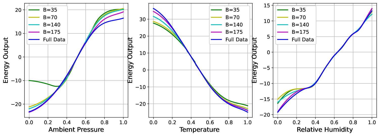
In this section, we apply the proposed methods to the Combined Cycle Power Plant Data (Kaya et al. 2012; Tüfekci 2014), which can be downloaded at http://https://archive.ics.uci.edu/ml/datasets/Combined+Cycle+Power+Plant. The data set consists of n=9568n=9568 observations from a Combined Cycle Power Plant over 6 years (2006-2011). The purpose of our analysis is to explore the relationship between the net hourly electrical energy output of the plant between three environmental factors: temperature, ambient pressure, and relative humidity.

Figure 6 displays the estimated curve based on BB-bits quantizations (B=35,70,140,175B=35,70,140,175) and full data, for which the periodic spline of order m=2m=2 was used. For the quantization step, we choose 𝒯n=2.5×σ^2​log⁡(n){\mathcal{T}}_{n}=2.5\times\hat{\sigma}^{2}\log(n), where σ^2\hat{\sigma}^{2} is the standard deviation of the observated data, and c,kc,k are determined by Section 2.5. We can observe that the spline estimator based on quantized data with B=35B=35, i.e., the green curve, is rather different from the other curves in the two analyzes. When the bits budget BB increases to more than 7070, such differences quickly diminish. This observation demonstrates the effectiveness of the proposed BB-bits quantization scheme.

Refer to caption
Figure 6: Spline estimators based on BB-bits quantizations (BB = 35,70,140,175) and full data. Sample size is n=9568n=9568.

Next, we conduct some hypothesis tests for the relationship between the net hourly electrical energy output and other three environmental factors. The first test is to test whether there is an association between the energy output and three environmental factors. We consider both non-adaptive and adaptive nonparametric tests. For the non-adaptive nonparametric test, m=2m=2 is used. The p-values are all close to zero, implying strong rejections of the null hypothesis. This is not surprising based on the shapes of the spline estimators illustrated in Figure 6.

Next, there appears to be a strong linear association between relative humidity and the energy output in Figure 6. Based on this conjecture, we proceed to test whether the associations between these three environmental factors and the energy output are linear or nonlinear, using the nonparametric linearity test proposed in Section 4.1. The p-values for the first two environmental factors, i.e., ambient pressure and temperature, are both close to zero, indicating strong rejections of the null hypothesis. Figure 7 illustrates the p-values of the nonparametric linearity test for the relationship between relative humidity and energy output as a function of the bits budget BB. We can see that the nonparametric linearity test based on quantized data fails to reject the null hypothesis, which echos our conjecture based on Figure 6.

Refer to caption
Figure 7: PP-values of the nonparametric linearity test for the relationship between relative humidity and energy output as a function of BB.

7 Discussion

In this paper, we propose a set of non-parametric testing procedures based on quantized observations, including the non-adaptive nonparametric test, the nonparametric linearity test, and the adaptive nonparametric test. The proposed tests are easy-to-use based on L2L_{2}-metric between the quantization spline estimators and the hypothesized function. We investigate the asymptotic validity and testing powers of the proposed tests and show how the asymptotic testing powers changes as the bits budget BB increases.

In the end, we discuss two additional extensions. First, the present paper only deals with periodic splines. It is interesting to extend our results to more general splines or even kernel ridge regression. The special periodic spline largely reduces the difficulty level of the technical proofs. Indeed, the majority of the proofs can be accomplished by exact calculations based on trigonometric series. For general RKHS, exact calculations may not be possible, and more involved proofs are needed. Second, the nonparametric linearity test can be easily extended to testing general composite null hypotheses such as H0general:g0​(x)=h0​(x,θ)H_{0}^{\textrm{general}}:g_{0}(x)=h_{0}(x,\theta) for some function h0h_{0} governed by parameters θ∈ℝp\theta\in\mathbb{R}^{p} with a fixed pp. However, when pp is diverging as nn increases, it will be more challenging to investigate the asymptotic behavior of the proposed test statistic and will be an interesting future research topic.

References

  • Adams and Fournier (2003) Robert A Adams and John JF Fournier. Sobolev spaces, volume 140. Elsevier, 2003.
  • Benhenni and Rachdi (2006) K Benhenni and Mustapha Rachdi. Nonparametric estimation of the regression function from quantized observations. Computational Statistics & Data Analysis, 50(11):3067–3085, 2006.
  • Boufounos and Baraniuk (2008) Petros T Boufounos and Richard G Baraniuk. 1-bit compressive sensing. Information Sciences and Systems, 2008. CISS 2008. 42nd Annual Conference on Information Sciences and Systems, pages 16–21, 2008.
  • Cai and Wei (2021) Tony Cai and Hongji Wei. Distributed nonparametric function estimation: Optimal rate of convergence and cost of adaptation. arXiv preprint arXiv:2107.00179, 2021.
  • Cheng and Shang (2015) Guang Cheng and Zuofeng Shang. Joint asymptotics for semi-nonparametric regression models with partially linear structure. The Annals of Statistics, 43(3):1351–1390, 2015.
  • Goldstein and Rinott (1996) Larry Goldstein and Yosef Rinott. Multivariate normal approximations by stein’s method and size bias couplings. Journal of Applied Probability, 33(1):1–17, 1996.
  • Gopi et al. (2013) Sivakant Gopi, Praneeth Netrapalli, Prateek Jain, and Aditya Nori. One-bit compressed sensing: Provable support and vector recovery. In International Conference on Machine Learning, pages 154–162, 2013.
  • Gu (2013) Chong Gu. Smoothing Spline ANOVA Models, volume 297. Springer Science & Business Media, 2013.
  • Gupta et al. (2010) Ankit Gupta, Robert Nowak, and Benjamin Recht. Sample complexity for 1-bit compressed sensing and sparse classification. In 2010 IEEE International Symposium on Information Theory, pages 1553–1557. IEEE, 2010.
  • Hall (1979) Peter Hall. On the rate of convergence of normal extremes. Journal of Applied Probability, 16(2):433–439, 1979.
  • Han et al. (2018) Yanjun Han, Pritam Mukherjee, Ayfer Ozgur, and Tsachy Weissman. Distributed statistical estimation of high-dimensional and nonparametric distributions. In 2018 IEEE International Symposium on Information Theory (ISIT), pages 506–510. IEEE, 2018.
  • Kaya et al. (2012) Heysem Kaya, Pmar Tüfekci, and Fikret S Gürgen. Local and global learning methods for predicting power of a combined gas & steam turbine. In Proceedings of the International Conference on Emerging Trends in Computer and Electronics Engineering Icetcee, pages 13–18, 2012.
  • Koike (2019) Yuta Koike. Gaussian approximation of maxima of Wiener functionals and its application to high-frequency data. The Annals of Statistics, 47(3):1663 – 1687, 2019.
  • Lee and Vardeman (2001) Chiang-Sheng Lee and Stephen B Vardeman. Interval estimation of a normal process mean from rounded data. Journal of Quality Technology, 33(3):335–348, 2001.
  • Liu et al. (2019) Meimei Liu, Zuofeng Shang, and Guang Cheng. Sharp theoretical analysis for nonparametric testing under random projection. In Conference on Learning Theory, pages 2175–2209, 2019.
  • Liu et al. (2020) Meimei Liu, Zuofeng Shang, and Guang Cheng. Nonparametric distributed learning under general designs. Electronic Journal of Statistics, 14:3070–3102, 2020.
  • Liu et al. (2021) Meimei Liu, Zuofeng Shang, Yun Yang, and Guang Cheng. Nonparametric testing under randomized sketching. IEEE Transactions on Pattern Analysis and Machine Intelligence, 2021.
  • Plan and Vershynin (2013) Yaniv Plan and Roman Vershynin. Robust 1-bit compressed sensing and sparse logistic regression: A convex programming approach. IEEE Transactions on Information Theory, 59(1):482–494, 2013.
  • Reinert and Röllin (2009) Gesine Reinert and Adrian Röllin. Multivariate normal approximation with stein’s method of exchangeable pairs under a general linearity condition. The Annals of Probability, 37(6):2150–2173, 2009.
  • Shang and Cheng (2013) Zuofeng Shang and Guang Cheng. Local and global asymptotic inference in smoothing spline models. The Annals of Statistics, 41(5):2608–2638, 2013.
  • Shang and Cheng (2015) Zuofeng Shang and Guang Cheng. Nonparametric inference in generalized functional linear models. The Annals of Statistics, 43(4):1742–1773, 2015.
  • Shang and Cheng (2017) Zuofeng Shang and Guang Cheng. Computational limits of a distributed algorithm for smoothing spline. The Journal of Machine Learning Research, 18(1):3809–3845, 2017.
  • Slawski and Li (2015) Martin Slawski and Ping Li. b-bit marginal regression. In Advances in Neural Information Processing Systems, pages 2062–2070, 2015.
  • Slawski and Li (2018) Martin Slawski and Ping Li. On the trade-off between bit depth and number of samples for a basic approach to structured signal recovery from bb-bit quantized linear measurements. IEEE Transactions on Information Theory, 64(6):4159–4178, 2018.
  • Suresh et al. (2017) Ananda Theertha Suresh, X Yu Felix, Sanjiv Kumar, and H Brendan McMahan. Distributed mean estimation with limited communication. In International Conference on Machine Learning, pages 3329–3337. PMLR, 2017.
  • Szabo and van Zanten (2020) Botond Szabo and Harry van Zanten. Adaptive distributed methods under communication constraints. The Annals of Statistics, 48(4):2347–2380, 2020.
  • Tsybakov (2008) Alexandre B. Tsybakov. Introduction to Nonparametric Estimation. Springer Publishing Company, Incorporated, 1st edition, 2008. ISBN 0387790519.
  • Tüfekci (2014) Pınar Tüfekci. Prediction of full load electrical power output of a base load operated combined cycle power plant using machine learning methods. International Journal of Electrical Power & Energy Systems, 60:126–140, 2014.
  • Vardeman and Lee (2005) Stephen B Vardeman and Chiang-Sheng Lee. Likelihood-based statistical estimation from quantized data. IEEE Transactions on Instrumentation and Measurement, 54(1):409–414, 2005.
  • Wahba (1990) Grace Wahba. Spline Models for Observational Data, volume 59. Siam, 1990.
  • Xu and Huang (2012) Ganggang Xu and Jianhua Z Huang. Asymptotic optimality and efficient computation of the leave-subject-out cross-validation. The Annals of Statistics, 40(6):3003–3030, 2012.
  • Xu et al. (2018) Ganggang Xu, Zuofeng Shang, and Guang Cheng. Optimal tuning for divide-and-conquer kernel ridge regression with massive data. In International Conference on Machine Learning, pages 5483–5491. PMLR, 2018.
  • Xu et al. (2019) Ganggang Xu, Zuofeng Shang, and Guang Cheng. Distributed generalized cross-validation for divide-and-conquer kernel ridge regression and its asymptotic optimality. Journal of computational and graphical statistics, 28(4):891–908, 2019.
  • Yang et al. (2020) Yun Yang, Zuofeng Shang, and Guang Cheng. Non-asymptotic analysis for nonparametric testing. In Jacob Abernethy and Shivani Agarwal, editors, Proceedings of Thirty Third Conference on Learning Theory, volume 125 of Proceedings of Machine Learning Research, pages 3709–3755. PMLR, 09–12 Jul 2020.
  • Zhang et al. (2014) Lijun Zhang, Jinfeng Yi, and Rong Jin. Efficient algorithms for robust one-bit compressive sensing. pages 820–828, 2014.
  • Zhang et al. (2013) Yuchen Zhang, John C Duchi, Michael I Jordan, and Martin J Wainwright. Information-theoretic lower bounds for distributed statistical estimation with communication constraints. In Advances in Neural Information Processing Systems, pages 2328–2336. Citeseer, 2013.
  • Zhu and Gu (2015) Rongda Zhu and Quanquan Gu. Towards a lower sample complexity for robust one-bit compressed sensing. In International Conference on Machine Learning, pages 739–747, 2015.
  • Zhu and Lafferty (2014) Yuancheng Zhu and John Lafferty. Quantized estimation of gaussian sequence models in euclidean balls. In Advances in Neural Information Processing Systems, pages 3662–3670, 2014.
  • Zhu and Lafferty (2017) Yuancheng Zhu and John Lafferty. Quantized minimax estimation over Sobolev ellipsoids. Information and Inference: A Journal of the IMA, 7(1):31–82, 2017.
  • Zhu and Lafferty (2018) Yuancheng Zhu and John Lafferty. Distributed nonparametric regression under communication constraints. In International Conference on Machine Learning, pages 6009–6017, 2018.

Appendix A Structure of the proofs

In this section, we outline the high-level structure of the proofs for the main theorems.

  • •

    The proof of Theorem 1 is mainly based on Lemma 10.

    • –

      In Lemma 10, we provide an upper bound for the difference between two smoothing spline estimators.

  • •

    The proof of Theorem 3 relies on Stein’s exchangeable pair method. Specifically, we first prove that the asymptotic normality of c​Tμ⋆,t,c−trace​(A)​τk⋆2sc​τk⋆2\frac{cT_{\mu^{\star},t,c}-\textrm{trace}(A)\tau^{\star 2}_{k}}{s_{c}\tau^{\star 2}_{k}} based on zi⋆z^{\star}_{i}’s, where zi⋆z^{\star}_{i}’s are the quantized samples corresponding to μj=μj⋆\mu_{j}=\mu^{\star}_{j} for 1≤j≤k1\leq j\leq k, τk⋆2=V​a​r​(zi⋆|H0)\tau^{\star 2}_{k}=Var(z^{\star}_{i}|H_{0}), and

    μj⋆=∑i=1nE⁡{yi​I​(yi∈Rj​(t))}∑i=1nP⁡(yi∈Rj​(t)).\mu^{\star}_{j}=\frac{\sum_{i=1}^{n}E\{y_{i}I(y_{i}\in R_{j}(t))\}}{\sum_{i=1}^{n}P(y_{i}\in R_{j}(t))}. (23)

    Next, we prove that

    c​Tμ⋆,t,c−trace​(A)​τk⋆2sc​τk⋆2−c​Tμ,t,c−trace​(A)​τ^k2sc​τ^k2=op​(1).\frac{cT_{\mu^{\star},t,c}-\textrm{trace}(A)\tau^{\star 2}_{k}}{s_{c}\tau^{\star 2}_{k}}-\frac{cT_{\mu,t,c}-\textrm{trace}(A)\widehat{\tau}_{k}^{2}}{s_{c}\widehat{\tau}_{k}^{2}}=o_{p}(1).
    • –

      In Lemma 11 and Lemma 12, we prove the error rate introduced by quantization of variance using Algorithm 2, which are needed for the proof of Theorem 3.

    • –

      In Lemma 13, we quantify the difference of quantized sample under H1H_{1} and H0H_{0}.

  • •

    In the proof of Theorem 5, we first decompose the test statistic into two parts,

    c​Tμ,t−trace​(A)​τ^k2sc​τ^k2=zT​A​z−(z0)T​A​z0sc​τ^k2+(z0)T​A​z0−trace​(A)​τ^k2sc​τ^k2,\frac{cT_{\mu,t}-\textrm{trace}(A)\widehat{\tau}_{k}^{2}}{s_{c}\widehat{\tau}_{k}^{2}}=\frac{z^{T}Az-(z^{0})^{T}Az^{0}}{s_{c}\widehat{\tau}_{k}^{2}}+\frac{(z^{0})^{T}Az^{0}-\textrm{trace}(A)\widehat{\tau}_{k}^{2}}{s_{c}\widehat{\tau}_{k}^{2}},

    where z0z^{0} is the vector of quantized sample under H0:g0=0H_{0}:g_{0}=0. Under Theorem 3, we know the second term is Op​(1)O_{p}(1). In the first term, it is straightforward to see that zT​A​z−(z0)T​A​z0=(z−z0)T​A​(z−z0)+2​(z−z0)T​A​z0z^{T}Az-(z^{0})^{T}Az^{0}=(z-z^{0})^{T}A(z-z^{0})+2(z-z^{0})^{T}Az^{0}.

    • –

      In Lemma 14, we establish a lower bound for (z−z0)T​A​z0(z-z^{0})^{T}Az^{0}.

    • –

      In Lemma 15 and Lemma 16, we establish the lower bound for (z−z0)T​A​(z−z0)(z-z^{0})^{T}A(z-z^{0}).

  • •

    In the proof of Theorem 8, observe that the test statistic for each mm

    ξm=c​Tm−trace​(Am)​τ^k2sc,m​τ^k2=(z0)T​Am​z0−trace​(Am)​τ^k2sc,m​τ^k2\xi_{m}=\frac{cT_{m}-\textrm{trace}(A_{m})\widehat{\tau}_{k}^{2}}{s_{c,m}\widehat{\tau}_{k}^{2}}=\frac{(z^{0})^{T}A_{m}z^{0}-\textrm{trace}(A_{m})\widehat{\tau}_{k}^{2}}{s_{c,m}\widehat{\tau}_{k}^{2}}

    is in a quadratic form.

    • –

      Lemma 17 proves that the maximum of the quadratic form follows an extreme value distribution.

    • –

      Lemma 18 provides the rate conditions such that Lemma 17 holds.

  • •

    The idea of Theorem 9 is similar to the proof of Theorem 5 and Theorem 7.

Appendix B Notation

In this section, we first summarize some notations which are frequently used through out the paper for the reader’s convenience.

Symbol Description
cc number of groups.
n~\widetilde{n} number of observations in each group which is defined as n~=n/c\widetilde{n}=n/c.
(μ1,…,μk)T(\mu_{1},\ldots,\mu_{k})^{T} quantized value.
(t1,…,tk−1)T(t_{1},\ldots,t_{k-1})^{T} cut-off points of quantized intervals.
y=(y1,…,yn)Ty=(y_{1},\ldots,y_{n})^{T} vector of response .
y~=(y~1,…,y~c)T\widetilde{y}=(\widetilde{y}_{1},\ldots,\widetilde{y}_{c})^{T} average of the response which is defined as y~i=1n~​∑j=(i−1)​n~+1i​n~yj\widetilde{y}_{i}=\frac{1}{\widetilde{n}}\sum_{j=(i-1)\widetilde{n}+1}^{i\widetilde{n}}y_{j}.
z=(z1,…,zc)Tz=(z_{1},\ldots,z_{c})^{T} vector of quantized sample.
z0=(z10,…,zc0)Tz^{0}=(z^{0}_{1},\ldots,z^{0}_{c})^{T} vector of quantized sample under H0:g0=0H_{0}:g_{0}=0.
z~=(z~1,…,z~c)T\widetilde{z}=(\widetilde{z}_{1},\ldots,\widetilde{z}_{c})^{T} vector of truncated quantized sample,
where z~i=zi𝟙(csρ+σ|ϵj|≤𝒯n) for all j=(i−1)n~+1,…in~)\widetilde{z}_{i}=z_{i}\mathbbm{1}(c_{s}\rho+\sigma|\epsilon_{j}|\leq\sqrt{{\mathcal{T}}_{n}})\textrm{ for all }j=(i-1)\widetilde{n}+1,\dots i\widetilde{n}).
z~0=(z~10,…,z~c0)T\widetilde{z}^{0}=(\widetilde{z}^{0}_{1},\ldots,\widetilde{z}^{0}_{c})^{T} vector of truncated quantized response under H0:g0=0H_{0}:g_{0}=0,
where z~i0=zi0𝟙(csρ+σ|ϵj|≤𝒯n) for all j=(i−1)n~+1,…in~)\widetilde{z}_{i}^{0}=z_{i}^{0}\mathbbm{1}(c_{s}\rho+\sigma|\epsilon_{j}|\leq\sqrt{{\mathcal{T}}_{n}})\textrm{ for all }j=(i-1)\widetilde{n}+1,\dots i\widetilde{n}).
ylinear=(y1linear,…,ynlinear)Ty^{\textrm{linear}}=(y_{1}^{\textrm{linear}},\ldots,y_{n}^{\textrm{linear}})^{T} new defined data for testing the linearity of g0g_{0}, which is defined as
yilinear=Q⁡(yi)−g^​(i/n)y_{i}^{\textrm{linear}}=Q(y_{i})-\widehat{g}(i/n), and g^​(i/n)\widehat{g}(i/n) is the least-square estimator of gg.
zlinear=(z1linear,…,zclinear)Tz^{\textrm{linear}}=(z_{1}^{\textrm{linear}},\ldots,z_{c}^{\textrm{linear}})^{T} vector of quantized value of yilineary_{i}^{\textrm{linear}}.
z0linear=(zi,0linear,…,zi,clinear)Tz_{0}^{\textrm{linear}}=(z_{i,0}^{\textrm{linear}},\ldots,z_{i,c}^{\textrm{linear}})^{T} quantized value of yilineary_{i}^{\textrm{linear}} under H0linear:g0​ is linear.H_{0}^{\textrm{linear}}:g_{0}\textrm{ is linear}.
λ\lambda smoothing parameter.
{φi​(x)}i=1∞\{\varphi_{i}(x)\}_{i=1}^{\infty} trigonometric basis functions.
K⁡(⋅,⋅)K(\cdot,\cdot) kernel function.
Σc\Sigma_{c} kernel matrix defined as Σc=[K⁡(i/c,i′/c)/c]1≤i,i′≤c\Sigma_{c}=[K(i/c,i^{\prime}/c)/c]_{1\leq i,i^{\prime}\leq c}.
Ωc\Omega_{c} “tensor” of K⁡(⋅,⋅)K(\cdot,\cdot) defined as Ωc=[K⊗2​(i/c,i′/c)/c]1≤i,i′≤c\Omega_{c}=[K^{\otimes 2}(i/c,i^{\prime}/c)/c]_{1\leq i,i^{\prime}\leq c}.
AA A=(Σc+λ​Ic)−1​Ωc​(Σc+λ​Ic)−1A=(\Sigma_{c}+\lambda I_{c})^{-1}\Omega_{c}(\Sigma_{c}+\lambda I_{c})^{-1}.
ζ\zeta approximation error of Riemann sum and integral.
csc_{s} Sobolev constant defined as cs=supf∈Sm​(𝕀)‖f‖supJ⁡(f)c_{s}=\sup_{f\in S^{m}(\mathbb{I})}\frac{\|f\|_{\sup}}{\sqrt{J(f)}}.
Ck​(t)C_{k}(t) maximum length of quantization interval.
Table 1: Table that lists some of the useful notations that are frequently used throughout the paper.

Appendix C Useful Lemmas

The proofs of the theorems require some preliminary lemmas. In this section, we summarize these useful lemmas. Throughout the proof, we let y~i=1n~∑j=(i−1)​n~+1i​n~yj,i=1,…,c\widetilde{y}_{i}=\frac{1}{\widetilde{n}}\sum_{j=(i-1)\widetilde{n}+1}^{i\widetilde{n}}y_{j},i=1,\ldots,c and we denote g^ss\widehat{g}^{\textrm{ss}} as the canonical smoothing spline based on the full dataset; g^css\widehat{g}^{\textrm{ss}}_{c} as the smoothing spline based on the averaged responses {y~1,⋯,y~c}\{\widetilde{y}_{1},\cdots,\widetilde{y}_{c}\}, and g^μ,t,cB\widehat{g}^{\textrm{B}}_{\mu,t,c} as the desired BB-bits estimator, i.e.,

g^ss\displaystyle\widehat{g}^{\textrm{ss}} =arg​ming∈Sm​(𝕀)⁡1n​∑i=1n(yi−g⁡(i/n))2+λ​∫01[g(m)​(x)]2​dx,\displaystyle=\argmin_{g\in S^{m}(\mathbb{I})}\frac{1}{n}\sum_{i=1}^{n}(y_{i}-g(i/n))^{2}+\lambda\int_{0}^{1}[g^{(m)}(x)]^{2}dx,
g^css\displaystyle\widehat{g}^{\textrm{ss}}_{c} =arg​ming∈Sm​(𝕀)⁡1c​∑i=1c(y~i−g⁡(i/c))2+λ​∫01[g(m)​(x)]2​dx,y~i=1n~​∑j=(i−1)​n~+1i​n~yj,\displaystyle=\argmin_{g\in S^{m}(\mathbb{I})}\frac{1}{c}\sum_{i=1}^{c}(\widetilde{y}_{i}-g(i/c))^{2}+\lambda\int_{0}^{1}[g^{(m)}(x)]^{2}dx,\,\,\,\widetilde{y}_{i}=\frac{1}{\widetilde{n}}\sum_{j=(i-1)\widetilde{n}+1}^{i\widetilde{n}}y_{j},
g^μ,t,cB\displaystyle\widehat{g}^{\textrm{B}}_{\mu,t,c} =arg​ming∈Sm​(𝕀)⁡1c​∑i=1c(zi−g⁡(i/c))2+λ​∫01[g(m)​(x)]2​dx.\displaystyle=\argmin_{g\in S^{m}(\mathbb{I})}\frac{1}{c}\sum_{i=1}^{c}(z_{i}-g(i/c))^{2}+\lambda\int_{0}^{1}[g^{(m)}(x)]^{2}dx.

The following lemma describes that the distance between g^μ,t,cB\widehat{g}^{\textrm{B}}_{\mu,t,c} and g^css\widehat{g}^{\textrm{ss}}_{c} can be well controlled by carefully choosing quantization parameters μ,t\mu,t and cc.

Lemma 10.

For any μ=(μ1,…,μk)T∈ℝk\mu=(\mu_{1},\ldots,\mu_{k})^{T}\in\mathbb{R}^{k} and t=(t1,…,tk−1)T∈ℝk−1t=(t_{1},\ldots,t_{k-1})^{T}\in\mathbb{R}^{k-1}, it holds that

‖g^μ,t,cB−g^css‖2≤c−1​∑i=1c(zi−y~i)2.\|\widehat{g}^{\textrm{B}}_{\mu,t,c}-\widehat{g}^{\textrm{ss}}_{c}\|^{2}\leq c^{-1}\sum_{i=1}^{c}(z_{i}-\widetilde{y}_{i})^{2}. (24)
Proof.

Recall that g^μ,t,cB=∑i=1cθ^i​Ki/c\widehat{g}^{\textrm{B}}_{\mu,t,c}=\sum_{i=1}^{c}\widehat{\theta}_{i}K_{i/c}, where (θ^1,…,θ^c)T=c−1​(Σc+λ​Ic)−1​z(\widehat{\theta}_{1},\ldots,\widehat{\theta}_{c})^{T}=c^{-1}(\Sigma_{c}+\lambda I_{c})^{-1}z with Σc=[K⁡(i/c,i′/c)/c]1≤i,i′≤c∈ℝc×c\Sigma_{c}=[K(i/c,i^{\prime}/c)/c]_{1\leq i,i^{\prime}\leq c}\in\mathbb{R}^{c\times c}, z=(z1,…,zc)T∈ℝcz=(z_{1},\ldots,z_{c})^{T}\in\mathbb{R}^{c}, and K⁡(⋅,⋅)K(\cdot,\cdot) is the kernel function. Similarly, g^css=∑i=1cθ~i​Ki/c\widehat{g}^{\textrm{ss}}_{c}=\sum_{i=1}^{c}\widetilde{\theta}_{i}K_{i/c}, where (θ~1,…,θ~c)T=c−1​(Σc+λ​Ic)−1​y~(\widetilde{\theta}_{1},\ldots,\widetilde{\theta}_{c})^{T}=c^{-1}(\Sigma_{c}+\lambda I_{c})^{-1}\widetilde{y} with y~=(y~1,…,y~c)T\widetilde{y}=(\widetilde{y}_{1},\ldots,\widetilde{y}_{c})^{T}. Let θ^=(θ^1,…,θ^c)T,θ~=(θ~1,…,θ~c)T\widehat{\theta}=(\widehat{\theta}_{1},\ldots,\widehat{\theta}_{c})^{T},\widetilde{\theta}=(\widetilde{\theta}_{1},\ldots,\widetilde{\theta}_{c})^{T}. By direct calculations, we have

g^μ,t,cB−g^css\displaystyle\widehat{g}_{\mu,t,c}^{\textrm{B}}-\widehat{g}^{\textrm{ss}}_{c} =\displaystyle= ∑ν=1∞∑i=1c(θ^i−θ~i)​φν​(i/c)γν​φν=∑ν=1∞ΦνT​(θ^−OPENθ)~CLOSEγν​φν,\displaystyle\sum_{\nu=1}^{\infty}\sum_{i=1}^{c}(\widehat{\theta}_{i}-\widetilde{\theta}_{i})\frac{\varphi_{\nu}(i/c)}{\gamma_{\nu}}\varphi_{\nu}=\sum_{\nu=1}^{\infty}\frac{\Phi_{\nu}^{T}(\widehat{\theta}-\widetilde{\theta)}}{\gamma_{\nu}}\varphi_{\nu},

where φ2​k−1​(x)=2​cos⁡(2​π​k​x),φ2​k​(x)=2​sin⁡(2​π​k​x)\varphi_{2k-1}(x)=\sqrt{2}\cos(2\pi kx),\,\,\,\,\varphi_{2k}(x)=\sqrt{2}\sin(2\pi kx) are the trigonometric basis functions, γ2​k−1=γ2​k=(2​π​k)2​m\gamma_{2k-1}=\gamma_{2k}=(2\pi k)^{2m}, and Φν=(φν​(1/c),φν​(2/c),…,φν​(c/c))T\Phi_{\nu}=(\varphi_{\nu}(1/c),\varphi_{\nu}(2/c),\ldots,\varphi_{\nu}(c/c))^{T}. So

‖g^μ,t,cB−g^css‖2\displaystyle\|\widehat{g}^{\textrm{B}}_{\mu,t,c}-\widehat{g}^{\textrm{ss}}_{c}\|^{2} =\displaystyle= ∑ν=1∞|ΦνT​(θ^−θ~)|2γν2\displaystyle\sum_{\nu=1}^{\infty}\frac{|\Phi_{\nu}^{T}(\widehat{\theta}-\widetilde{\theta})|^{2}}{\gamma_{\nu}^{2}} (25)
=\displaystyle= (θ^−θ~)T​∑ν=1∞Φν​ΦνTγν2​(θ^−θ~)\displaystyle(\widehat{\theta}-\widetilde{\theta})^{T}\sum_{\nu=1}^{\infty}\frac{\Phi_{\nu}\Phi_{\nu}^{T}}{\gamma_{\nu}^{2}}(\widehat{\theta}-\widetilde{\theta})
=\displaystyle= c−1​(z−y~)T​(Σc+λ​Ic)−1​Ωc​(Σc+λ​Ic)−1​(z−y~).\displaystyle c^{-1}(z-\widetilde{y})^{T}(\Sigma_{c}+\lambda I_{c})^{-1}\Omega_{c}(\Sigma_{c}+\lambda I_{c})^{-1}(z-\widetilde{y}).

We now look at Σc\Sigma_{c} and Ωc\Omega_{c}. To ease our calculations, for 0≤l≤c−10\leq l\leq c-1, we first define the following two notations,

dl′\displaystyle d^{\prime}_{l} =\displaystyle= 2c​∑k=1∞cos⁡(2​π​k​l/c)(2​π​k)2​m,dl=2c​∑k=1∞cos⁡(2​π​k​l/c)(2​π​k)4​m.\displaystyle\frac{2}{c}\sum_{k=1}^{\infty}\frac{\cos(2\pi kl/c)}{(2\pi k)^{2m}},d_{l}=\frac{2}{c}\sum_{k=1}^{\infty}\frac{\cos(2\pi kl/c)}{(2\pi k)^{4m}}.

Since dl′=dc−l′d^{\prime}_{l}=d^{\prime}_{c-l}, dl=dc−ld_{l}=d_{c-l} for l=1,2,…,c−1l=1,2,\ldots,c-1, we know Σc,Ωc\Sigma_{c},\Omega_{c} are both symmetric circulant of order cc. Furthermore, Σc\Sigma_{c} and Ωc\Omega_{c} share the same normalized eigenvectors as

xr=1c(1,εr,ε2​r,…,ε(c−1)​r)T,r=0,1,…,c−1,x_{r}=\frac{1}{\sqrt{c}}(1,\varepsilon^{r},\varepsilon^{2r},\ldots,\varepsilon^{(c-1)r})^{T},\,\,r=0,1,\ldots,c-1,

where ε=exp⁡(2​π​−1/c)\varepsilon=\exp(2\pi\sqrt{-1}/c). Let M=(x0,x1,…,xc−1)M=(x_{0},x_{1},\ldots,x_{c-1}), and M∗M^{\ast} be the conjugate transpose of MM. Clearly, M​M∗=IcMM^{\ast}=I_{c} and Σc,Ωc\Sigma_{c},\Omega_{c} admit the following decomposition

Σc=M​Λd′​M∗,Ωc=M​Λd​M∗,\Sigma_{c}=M\Lambda_{d^{\prime}}M^{\ast},\,\,\Omega_{c}=M\Lambda_{d}M^{\ast}, (26)

where Λd′=diag​(λd′,0,λd′,1,…,λd′,c−1)\Lambda_{d^{\prime}}=\textrm{diag}(\lambda_{d^{\prime},0},\lambda_{d^{\prime},1},\ldots,\lambda_{d^{\prime},c-1}) and Λd=diag​(λd,0,λd,1,…,λd,c−1)\Lambda_{d}=\textrm{diag}(\lambda_{d,0},\lambda_{d,1},\ldots,\lambda_{d,c-1}) with λd′,l=d0′+d1′​εl+…+dc−1′​ε(c−1)​l\lambda_{d^{\prime},l}=d^{\prime}_{0}+d^{\prime}_{1}\varepsilon^{l}+\ldots+d^{\prime}_{c-1}\varepsilon^{(c-1)l} and λd,l=d0+d1​εl+…+dc−1​ε(c−1)​l\lambda_{d,l}=d_{0}+d_{1}\varepsilon^{l}+\ldots+d_{c-1}\varepsilon^{(c-1)l}.

Direct calculations show that

λd′,l={2​∑k=1∞1(2​π​k​c)2​m,l=0,∑k=1∞1[2​π​(k​c−l)]2​m+∑k=0∞1[2​π​(k​c+l)]2​m,1≤l≤c−1\lambda_{d^{\prime},l}=\left\{\begin{array}[]{cc}2\sum_{k=1}^{\infty}\frac{1}{(2\pi kc)^{2m}},&l=0,\\ \sum_{k=1}^{\infty}\frac{1}{[2\pi(kc-l)]^{2m}}+\sum_{k=0}^{\infty}\frac{1}{[2\pi(kc+l)]^{2m}},&1\leq l\leq c-1\end{array}\right.
λd,l={2​∑k=1∞1(2​π​k​c)4​m,l=0,∑k=1∞1[2​π​(k​c−l)]4​m+∑k=0∞1[2​π​(k​c+l)]4​m,1≤l≤c−1.\lambda_{d,l}=\left\{\begin{array}[]{cc}2\sum_{k=1}^{\infty}\frac{1}{(2\pi kc)^{4m}},&l=0,\\ \sum_{k=1}^{\infty}\frac{1}{[2\pi(kc-l)]^{4m}}+\sum_{k=0}^{\infty}\frac{1}{[2\pi(kc+l)]^{4m}},&1\leq l\leq c-1.\end{array}\right.

It is easy to examine that

λd′,l={2​d′¯m​(2​π​c)−2​m,l=0,1[2​π​(c−l)]2​m+1(2​π​l)2​m+∑k=2∞1[2​π​(k​c−l)]2​m+∑k=1∞1[2​π​(k​c+l)]2​m,1≤l≤c−1,\lambda_{d^{\prime},l}=\left\{\begin{array}[]{cc}2\bar{d^{\prime}}_{m}(2\pi c)^{-2m},&l=0,\\ \frac{1}{[2\pi(c-l)]^{2m}}+\frac{1}{(2\pi l)^{2m}}+\sum_{k=2}^{\infty}\frac{1}{[2\pi(kc-l)]^{2m}}+\sum_{k=1}^{\infty}\frac{1}{[2\pi(kc+l)]^{2m}},&1\leq l\leq c-1,\end{array}\right. (27)
λd,l={2​d¯m​(2​π​c)−4​m,l=0,1[2​π​(c−l)]4​m+1(2​π​l)4​m+∑k=2∞1[2​π​(k​c−l)]4​m+∑k=1∞1[2​π​(k​c+l)]4​m,1≤l≤c−1,\lambda_{d,l}=\left\{\begin{array}[]{cc}2\bar{d}_{m}(2\pi c)^{-4m},&l=0,\\ \frac{1}{[2\pi(c-l)]^{4m}}+\frac{1}{(2\pi l)^{4m}}+\sum_{k=2}^{\infty}\frac{1}{[2\pi(kc-l)]^{4m}}+\sum_{k=1}^{\infty}\frac{1}{[2\pi(kc+l)]^{4m}},&1\leq l\leq c-1,\end{array}\right. (28)
d¯m′​(2​π​c)−2​m≤∑k=2∞1[2​π​(k​c−l)]2​m≤d′¯m​(2​π​c)−2​m,\displaystyle\underline{d}^{\prime}_{m}(2\pi c)^{-2m}\leq\sum_{k=2}^{\infty}\frac{1}{[2\pi(kc-l)]^{2m}}\leq\bar{d^{\prime}}_{m}(2\pi c)^{-2m},
d¯m′​(2​π​c)−2​m≤∑k=1∞1[2​π​(k​c+l)]2​m≤d¯m′​(2​π​c)−2​m,\displaystyle\underline{d}^{\prime}_{m}(2\pi c)^{-2m}\leq\sum_{k=1}^{\infty}\frac{1}{[2\pi(kc+l)]^{2m}}\leq\bar{d}^{\prime}_{m}(2\pi c)^{-2m},
d¯m​(2​π​c)−4​m≤∑k=2∞1[2​π​(k​c−l)]4​m≤d¯m​(2​π​c)−4​m,\displaystyle\underline{d}_{m}(2\pi c)^{-4m}\leq\sum_{k=2}^{\infty}\frac{1}{[2\pi(kc-l)]^{4m}}\leq\bar{d}_{m}(2\pi c)^{-4m},
d¯m​(2​π​c)−4​m≤∑k=1∞1[2​π​(k​c+l)]4​m≤d¯m​(2​π​c)−4​m,\displaystyle\underline{d}_{m}(2\pi c)^{-4m}\leq\sum_{k=1}^{\infty}\frac{1}{[2\pi(kc+l)]^{4m}}\leq\bar{d}_{m}(2\pi c)^{-4m},

where

d¯m′:=∑k=1∞k−2​m,d¯m′:=∑k=2∞k−2​m,d¯m:=∑k=1∞k−4​m,d¯m:=∑k=2∞k−4​m.\displaystyle\bar{d}^{\prime}_{m}:=\sum_{k=1}^{\infty}k^{-2m},\underline{d}^{\prime}_{m}:=\sum_{k=2}^{\infty}k^{-2m},\bar{d}_{m}:=\sum_{k=1}^{\infty}k^{-4m},\underline{d}_{m}:=\sum_{k=2}^{\infty}k^{-4m}. (29)

It follows from (27) and (28) that λd,l≤λd′,l2\lambda_{d,l}\leq\lambda_{d^{\prime},l}^{2} for 0≤l≤c−10\leq l\leq c-1. Therefore,

(z−y~)T​(Σc+λ​Ic)−1​Ωc​(Σc+λ​Ic)−1​(z−y~)\displaystyle(z-\widetilde{y})^{T}(\Sigma_{c}+\lambda I_{c})^{-1}\Omega_{c}(\Sigma_{c}+\lambda I_{c})^{-1}(z-\widetilde{y})
=\displaystyle= (z−y~)T​M​diag​(λd,0(λ+λd′,0)2,…,λd,c−1(λ+λd′,c−1)2)​M∗​(z−y~)\displaystyle(z-\widetilde{y})^{T}M\textrm{diag}\left(\frac{\lambda_{d,0}}{(\lambda+\lambda_{d^{\prime},0})^{2}},\ldots,\frac{\lambda_{d,c-1}}{(\lambda+\lambda_{d^{\prime},c-1})^{2}}\right)M^{\ast}(z-\widetilde{y})
≤\displaystyle\leq (z−y~)T​M​M∗​(z−y~)=(z−y~)T​(z−y~).\displaystyle(z-\widetilde{y})^{T}MM^{\ast}(z-\widetilde{y})=(z-\widetilde{y})^{T}(z-\widetilde{y}).

Therefore, it follows by (25) that

‖g^μ,t,cB−g^css‖2≤c−1​(z−y~)T​(z−y~)=c−1​∑i=1c(zi−y~i)2.\begin{split}\|\widehat{g}^{\textrm{B}}_{\mu,t,c}-\widehat{g}^{\textrm{ss}}_{c}\|^{2}\leq c^{-1}(z-\widetilde{y})^{T}(z-\widetilde{y})=c^{-1}\sum_{i=1}^{c}(z_{i}-\widetilde{y}_{i})^{2}.\end{split} (30)

This completes the proof. ∎

Lemma 11.

Suppose Condition (B) holds true, and it holds that Ck​(t)→0C_{k}(t)\rightarrow{0}, then we have τk2=V​a​r​(z1|H0)=O⁡(n~−1+Ck​(t)2)\tau_{k}^{2}=Var(z_{1}|H_{0})=O(\widetilde{n}^{-1}+C_{k}(t)^{2}) and τ^k2=τ~n22​n~​(n−1)=τk2[1+Op(n−1/2+Ck(t))]=τk2[1+op(1)]\widehat{\tau}_{k}^{2}=\frac{\widetilde{\tau}_{n}^{2}}{2\widetilde{n}(n-1)}=\tau_{k}^{2}\left[1+O_{p}(n^{-1/2}+C_{k}(t))\right]=\tau_{k}^{2}[1+o_{p}(1)].

Proof.

By the definition of τk2\tau_{k}^{2} and (6) we have

τk2\displaystyle\tau_{k}^{2} =V​a​r​(z1|H0)=1n~2​V​a​r​(∑i=1n~Q⁡(yi)|H0)+O⁡(Ck​(t)2)=1n~​V​a​r​(Q⁡(σ​ϵ1))+O⁡(Ck​(t)2)\displaystyle=Var(z_{1}|H_{0})=\frac{1}{\widetilde{n}^{2}}Var(\sum_{i=1}^{\widetilde{n}}Q(y_{i})|H_{0})+O(C_{k}(t)^{2})=\frac{1}{\widetilde{n}}Var(Q(\sigma\epsilon_{1}))+O(C_{k}(t)^{2})
=1n~​∑j=1kμj2​P​(Q⁡(σ​ϵ1)=μj)−1n~​(∑j=1kμj​P​(Q⁡(σ​ϵ1)=μj))2+O⁡(Ck​(t)2)\displaystyle=\frac{1}{\widetilde{n}}\sum_{j=1}^{k}\mu_{j}^{2}P\left(Q(\sigma\epsilon_{1})=\mu_{j}\right)-\frac{1}{\widetilde{n}}\left(\sum_{j=1}^{k}\mu_{j}P\left(Q(\sigma\epsilon_{1})=\mu_{j}\right)\right)^{2}+O(C_{k}(t)^{2})
=1n~​∑j=1kμj2​P​(σ​ϵ1∈Rj​(t))−1n~​(∑j=1kμj​P​(σ​ϵ1∈Rj​(t)))2+O⁡(Ck​(t)2)\displaystyle=\frac{1}{\widetilde{n}}\sum_{j=1}^{k}\mu_{j}^{2}P\left(\sigma\epsilon_{1}\in R_{j}(t)\right)-\frac{1}{\widetilde{n}}\left(\sum_{j=1}^{k}\mu_{j}P\left(\sigma\epsilon_{1}\in R_{j}(t)\right)\right)^{2}+O(C_{k}(t)^{2})
=R1+R2+O⁡(Ck​(t)2).\displaystyle=R_{1}+R_{2}+O(C_{k}(t)^{2}). (31)

Assume that for 2≤s≤k−1,t1<t2<⋯<ts−1≤0<ts<⋯<tk−12\leq s\leq k-1,t_{1}<t_{2}<\cdots<t_{s-1}\leq 0<t_{s}<\cdots<t_{k-1} and let p⁡(ϵ)p(\epsilon) be the density function of ϵ1\epsilon_{1}. Then we have

∑j=2s−1μj2​P​(σ​ϵ1∈Rj​(t))\displaystyle\sum_{j=2}^{s-1}\mu_{j}^{2}P\left(\sigma\epsilon_{1}\in R_{j}(t)\right) ≤∑j=2s−1∫tj−1/σtj/σp⁡(ϵ)​dϵ​tj−12\displaystyle\leq\sum_{j=2}^{s-1}\int_{t_{j-1}/\sigma}^{t_{j}/\sigma}p(\epsilon)d\epsilon t_{j-1}^{2}
≤2​∑j=2s−1∫tj−1/σtj/σp⁡(ϵ)​dϵ​(tj2+Ck​(t)2)\displaystyle\leq 2\sum_{j=2}^{s-1}\int_{t_{j-1}/\sigma}^{t_{j}/\sigma}p(\epsilon)d\epsilon\left(t_{j}^{2}+C_{k}\left(t\right)^{2}\right)
≤2​σ2​∑j=2s−1∫tj−1/σtj/σϵ2​p​(ϵ)​𝑑ϵ+2​Ck​(t)2​∑j=2s−1∫tj−1/σtj/σp⁡(ϵ)​𝑑ϵ\displaystyle\leq 2\sigma^{2}\sum_{j=2}^{s-1}\int_{t_{j-1}/\sigma}^{t_{j}/\sigma}\epsilon^{2}p(\epsilon)d\epsilon+2C_{k}(t)^{2}\sum_{j=2}^{s-1}\int_{t_{j-1}/\sigma}^{t_{j}/\sigma}p(\epsilon)d\epsilon

and

∑j=s+1k−1μj2​P​(σ​ϵ1∈Rj​(t))\displaystyle\sum_{j=s+1}^{k-1}\mu_{j}^{2}P\left(\sigma\epsilon_{1}\in R_{j}(t)\right) ≤∑j=s+1k−1∫tj−1/σtj/σp⁡(ϵ)​dϵ​tj2\displaystyle\leq\sum_{j=s+1}^{k-1}\int_{t_{j-1}/\sigma}^{t_{j}/\sigma}p(\epsilon)d\epsilon t_{j}^{2}
≤2​∑j=s+1k−1∫tj−1/σtj/σp⁡(ϵ)​dϵ​(tj−12+Ck​(t)2)\displaystyle\leq 2\sum_{j=s+1}^{k-1}\int_{t_{j-1}/\sigma}^{t_{j}/\sigma}p(\epsilon)d\epsilon\left(t_{j-1}^{2}+C_{k}(t)^{2}\right)
≤2​σ2​∑j=s+1k−1∫tj−1/σtj/σϵ2​p​(ϵ)​dϵ+2​Ck​(t)2​∑j=s+1k−1∫tj−1/σtj/σp⁡(ϵ)​dϵ.\displaystyle\leq 2\sigma^{2}\sum_{j=s+1}^{k-1}\int_{t_{j-1}/\sigma}^{t_{j}/\sigma}\epsilon^{2}p(\epsilon)d\epsilon+2C_{k}(t)^{2}\sum_{j=s+1}^{k-1}\int_{t_{j-1}/\sigma}^{t_{j}/\sigma}p(\epsilon)d\epsilon.

The fact that |μs|≤Ck​(t)\left|\mu_{s}\right|\leq C_{k}(t) and the above inequalities lead

R1=\displaystyle R_{1}= 1n~{∑j=2s−1μj2P(σϵ1∈Rj(t))+∑j=s+1k−1μj2P(σϵ1∈Rj(t))\displaystyle\frac{1}{\widetilde{n}}\Bigg\{\sum_{j=2}^{s-1}\mu_{j}^{2}P\left(\sigma\epsilon_{1}\in R_{j}(t)\right)+\sum_{j=s+1}^{k-1}\mu_{j}^{2}P\left(\sigma\epsilon_{1}\in R_{j}(t)\right)
+μ12P(σϵ1∈R1(t))+μk2P(σϵ1∈Rk(t))+μs2P(σϵ1∈Rs(t))}\displaystyle+\mu_{1}^{2}P\left(\sigma\epsilon_{1}\in R_{1}(t)\right)+\mu_{k}^{2}P\left(\sigma\epsilon_{1}\in R_{k}(t)\right)+\mu_{s}^{2}P\left(\sigma\epsilon_{1}\in R_{s}(t)\right)\Bigg\}
≤\displaystyle\leq 1n~​{2​σ2​∫ℝϵ2​p​(ϵ)​dϵ+3​Ck​(t)2+O⁡(1)}.\displaystyle\frac{1}{\widetilde{n}}\left\{2\sigma^{2}\int_{\mathbb{R}}\epsilon^{2}p(\epsilon)d\epsilon+3C_{k}(t)^{2}+O(1)\right\}.

This proves R1≲1n~R_{1}\lesssim\frac{1}{\widetilde{n}}. On the other hand, by t12>σ2t_{1}^{2}>\sigma^{2} and ts−1=O⁡(Ck​(t))=o⁡(1)t_{s-1}=O\left(C_{k}(t)\right)=o(1), we have

R1\displaystyle R_{1} ≥1n~​∑j=2s−1μj2​P​(σ​ϵ1∈Rj​(t))\displaystyle\geq\frac{1}{\widetilde{n}}\sum_{j=2}^{s-1}\mu_{j}^{2}P\left(\sigma\epsilon_{1}\in R_{j}(t)\right)
≥1n~​∑j=2s−1tj2​∫tj−1/σtj/σp⁡(ϵ)​𝑑ϵ\displaystyle\geq\frac{1}{\widetilde{n}}\sum_{j=2}^{s-1}t_{j}^{2}\int_{t_{j-1}/\sigma}^{t_{j}/\sigma}p(\epsilon)d\epsilon
≥1n~​∑j=2s−1(tj−12/2−Ck​(t)2)​∫tj−1/σtj/σp⁡(ϵ)​𝑑ϵ\displaystyle\geq\frac{1}{\widetilde{n}}\sum_{j=2}^{s-1}\left(t_{j-1}^{2}/2-C_{k}(t)^{2}\right)\int_{t_{j-1}/\sigma}^{t_{j}/\sigma}p(\epsilon)d\epsilon
≥1n~​{σ22​∑j=2s−1∫tj−1/σtj/σϵ2​p​(ϵ)​dϵ−Ck​(t)2​∑j=2s−1∫tj−1/σtj/σp⁡(ϵ)​dϵ}\displaystyle\geq\frac{1}{\widetilde{n}}\left\{\frac{\sigma^{2}}{2}\sum_{j=2}^{s-1}\int_{t_{j-1}/\sigma}^{t_{j}/\sigma}\epsilon^{2}p(\epsilon)d\epsilon-C_{k}(t)^{2}\sum_{j=2}^{s-1}\int_{t_{j-1}/\sigma}^{t_{j}/\sigma}p(\epsilon)d\epsilon\right\}
≥1n~​{σ22​∫t1/σts−1/σϵ2​p​(ϵ)​dϵ−Ck​(t)2}=O⁡(n~−1).\displaystyle\geq\frac{1}{\widetilde{n}}\left\{\frac{\sigma^{2}}{2}\int_{t_{1}/\sigma}^{t_{s-1}/\sigma}\epsilon^{2}p(\epsilon)d\epsilon-C_{k}(t)^{2}\right\}=O(\widetilde{n}^{-1}).

This proves R1≳1n~R_{1}\gtrsim\frac{1}{\widetilde{n}}, which implies R1=O⁡(n~−1)R_{1}=O(\widetilde{n}^{-1}). Using a similar approach, we can prove R2=O⁡(n~−1)R_{2}=O(\widetilde{n}^{-1}). From (C), we get τk2=O⁡(n~−1+Ck​(t)2)\tau_{k}^{2}=O(\widetilde{n}^{-1}+C_{k}(t)^{2}).

Now we prove τ^k2=τ~n22​n~​(n−1)=τk2​[1+op​(1)]\widehat{\tau}_{k}^{2}=\frac{\widetilde{\tau}_{n}^{2}}{2\widetilde{n}(n-1)}=\tau_{k}^{2}[1+o_{p}(1)]. By the definition of τ~n\widetilde{\tau}_{n}, we have

τ~n22​n~​(n−1)\displaystyle\frac{\widetilde{\tau}_{n}^{2}}{2\widetilde{n}(n-1)} =12​n~​(n−1)​∑i=2n(Q⁡(yi)−Q⁡(yi−1))2\displaystyle=\frac{1}{2\widetilde{n}(n-1)}\sum_{i=2}^{n}(Q(y_{i})-Q(y_{i-1}))^{2}
=12​n~​(n−1)​∑i=2n{Q⁡(g0​(i/n)+σ​ϵi)−Q⁡(g0​((i−1)/n)+σ​ϵi−1)}2\displaystyle=\frac{1}{2\widetilde{n}(n-1)}\sum_{i=2}^{n}\left\{Q(g_{0}(i/n)+\sigma\epsilon_{i})-Q(g_{0}((i-1)/n)+\sigma\epsilon_{i-1})\right\}^{2}
=12​n~​(n−1)​∑i=2n{g0​(i/n)−g0​((i−1)/n)+Q⁡(σ​ϵi)−Q⁡(σ​ϵi−1)+δ~i}2\displaystyle=\frac{1}{2\widetilde{n}(n-1)}\sum_{i=2}^{n}\left\{g_{0}(i/n)-g_{0}((i-1)/n)+Q(\sigma\epsilon_{i})-Q(\sigma\epsilon_{i-1})+\widetilde{\delta}_{i}\right\}^{2}
=12​n~​(n−1)​∑i=2n{Q⁡(σ​ϵi)−Q⁡(σ​ϵi−1)}2+12​n~​(n−1)​∑i=2n{g0​(i/n)−g0​((i−1)/n)+δ~i}2\displaystyle=\frac{1}{2\widetilde{n}(n-1)}\sum_{i=2}^{n}\left\{Q(\sigma\epsilon_{i})-Q(\sigma\epsilon_{i-1})\right\}^{2}+\frac{1}{2\widetilde{n}(n-1)}\sum_{i=2}^{n}\left\{g_{0}(i/n)-g_{0}((i-1)/n)+\widetilde{\delta}_{i}\right\}^{2}
+1n~​(n−1)∑i=2n{Q(σϵi)−Q(σϵi−1)}{g0(i/n)−g0((i−1)/n)+δ~i},\displaystyle\qquad+\frac{1}{\widetilde{n}(n-1)}\sum_{i=2}^{n}\left\{Q(\sigma\epsilon_{i})-Q(\sigma\epsilon_{i-1})\right\}\left\{g_{0}(i/n)-g_{0}((i-1)/n)+\widetilde{\delta}_{i}\right\},

where |δ~i|=O⁡(Ck​(t))|\widetilde{\delta}_{i}|=O(C_{k}(t)) for i=1,⋯,ni=1,\cdots,n. Note that, by the central limit theorem, it holds that

12​(n−1)∑i=2n{Q(σϵi)−Q(σϵi−1)}2=Var[Q(σϵ1)]+Op(n−1/2),\frac{1}{2(n-1)}\sum_{i=2}^{n}\left\{Q(\sigma\epsilon_{i})-Q(\sigma\epsilon_{i-1})\right\}^{2}=Var\left[Q(\sigma\epsilon_{1})\right]+O_{p}(n^{-1/2}),

and that g0​(i/n)−g0​((i−1)/n)=O⁡(1/n)g_{0}(i/n)-g_{0}((i-1)/n)=O(1/n) by the smoothness of function g0g_{0}, we have that

τ~n22​n~​(n−1)\displaystyle\frac{\widetilde{\tau}_{n}^{2}}{2\widetilde{n}(n-1)} =1n~[Var(Q(σϵ1))+O(n−2+Ck(t)2)+Op(n−1/2)+O(n−1+Ck(t))]\displaystyle=\frac{1}{\widetilde{n}}\left[Var(Q(\sigma\epsilon_{1}))+O(n^{-2}+C_{k}(t)^{2})+O_{p}(n^{-1/2})+O(n^{-1}+C_{k}(t))\right]
=τk2[1+Op(n−1/2+Ck(t))],\displaystyle=\tau_{k}^{2}\left[1+O_{p}(n^{-1/2}+C_{k}(t))\right], (32)

which completes the proof. ∎

Lemma 12.

Suppose Condition (B) holds true, and it holds that Ck​(t)→0C_{k}(t)\rightarrow{0}. Let τ^k2\widehat{\tau}_{k}^{2} be the quantied variance based on ylineary^{\textrm{linear}}, then we have that τ^k2=τ~n22​n~​(n−1)=τk2[1+Op(n−1/2+Ck(t))]=τk2[1+op(1)]\widehat{\tau}_{k}^{2}=\frac{\widetilde{\tau}_{n}^{2}}{2\widetilde{n}(n-1)}=\tau_{k}^{2}\left[1+O_{p}(n^{-1/2}+C_{k}(t))\right]=\tau_{k}^{2}[1+o_{p}(1)].

Proof.

By the definition of τ^k2\widehat{\tau}_{k}^{2}, we have

τ~n22​n~​(n−1)\displaystyle\frac{\widetilde{\tau}_{n}^{2}}{2\widetilde{n}(n-1)} =12​n~​(n−1)​∑i=2n(Q⁡(yilinear)−Q⁡(yi−1linear))2\displaystyle=\frac{1}{2\widetilde{n}(n-1)}\sum_{i=2}^{n}(Q(y_{i}^{\textrm{linear}})-Q(y^{\textrm{linear}}_{i-1}))^{2}
=12​n~​(n−1)​∑i=2n{Q⁡[Q⁡(g0​(i/n)+σ​ϵi)−y^i]−Q⁡[Q⁡(g0​((i−1)/n)+σ​ϵi−1)]−y^i−1}2\displaystyle=\frac{1}{2\widetilde{n}(n-1)}\sum_{i=2}^{n}\left\{Q[Q(g_{0}(i/n)+\sigma\epsilon_{i})-\widehat{y}_{i}]-Q[Q(g_{0}((i-1)/n)+\sigma\epsilon_{i-1})]-\widehat{y}_{i-1}\right\}^{2}
=12​n~​(n−1)​∑i=2n{g0​(i/n)−g0​((i−1)/n)+y^i−y^i−1+Q⁡(σ​ϵi)−Q⁡(σ​ϵi−1)+δ~i}2,\displaystyle=\frac{1}{2\widetilde{n}(n-1)}\sum_{i=2}^{n}\left\{g_{0}(i/n)-g_{0}((i-1)/n)+\widehat{y}_{i}-\widehat{y}_{i-1}+Q(\sigma\epsilon_{i})-Q(\sigma\epsilon_{i-1})+\widetilde{\delta}_{i}\right\}^{2},

where |δ~i|=O⁡(Ck​(t))|\widetilde{\delta}_{i}|=O(C_{k}(t)) for i=1,⋯,ni=1,\cdots,n. Note that g^∈ℒ⁡(𝕀)\widehat{g}\in\mathcal{L}(\mathbb{I}), one has that |y^i−y^i−1|=Op​(1/n)|\widehat{y}_{i}-\widehat{y}_{i-1}|=O_{p}(1/n) by the smoothness of g^\widehat{g}. Similar to the proof in Lemma 11, we get τ^k2=τ~n22​n~​(n−1)=τk2[1+Op(n−1/2+Ck(t))]=τk2[1+op(1)]\widehat{\tau}_{k}^{2}=\frac{\widetilde{\tau}_{n}^{2}}{2\widetilde{n}(n-1)}=\tau_{k}^{2}\left[1+O_{p}(n^{-1/2}+C_{k}(t))\right]=\tau_{k}^{2}[1+o_{p}(1)]. ∎

To ease calculation, we define some useful notations. Let zi0z_{i}^{0} be the quantized data conditional on g0​(x)=0g_{0}(x)=0 and z0=(z10,…,zc0)Tz^{0}=(z_{1}^{0},\ldots,z_{c}^{0})^{T}. According to (6), we have

|zi0−1n~​∑j=(i−1)​n~+1i​n~Q⁡(σ​ϵj)|≤Ck​(t), for i=1,…,c.\left|z_{i}^{0}-\frac{1}{\widetilde{n}}\sum_{j=(i-1)\widetilde{n}+1}^{i\widetilde{n}}Q(\sigma\epsilon_{j})\right|\leq C_{k}(t),\,\,\textrm{ for $i=1,\ldots,c$.} (33)

Furthermore, we let z~0=(z~10,…,z~c0)T,z~=(z~1,…,z~c)T\widetilde{z}^{0}=(\widetilde{z}_{1}^{0},\ldots,\widetilde{z}_{c}^{0})^{T},\widetilde{z}=(\widetilde{z}_{1},\ldots,\widetilde{z}_{c})^{T}, where for i=1,…,c,i=1,\ldots,c,

z~i0=zi0𝟙(csρ+σ|ϵj|≤𝒯n for all j=(i−1)n~+1,…in~),\displaystyle\widetilde{z}_{i}^{0}=z_{i}^{0}\mathbbm{1}(c_{s}\rho+\sigma|\epsilon_{j}|\leq\sqrt{{\mathcal{T}}_{n}}\textrm{ for all }j=(i-1)\widetilde{n}+1,\dots i\widetilde{n}),
z~i=zi𝟙(csρ+σ|ϵj|≤𝒯n for all j=(i−1)n~+1,…in~).\displaystyle\widetilde{z}_{i}=z_{i}\mathbbm{1}(c_{s}\rho+\sigma|\epsilon_{j}|\leq\sqrt{{\mathcal{T}}_{n}}\textrm{ for all }j=(i-1)\widetilde{n}+1,\dots i\widetilde{n}).
Lemma 13.

Suppose gg is the regression function generating the samples. Suppose Condition (B) holds and σ​|ϵj|+cs​ρ≤𝒯n\sigma|\epsilon_{j}|+c_{s}\rho\leq\sqrt{{\mathcal{T}}_{n}} holds for all j=1,…,nj=1,\ldots,n. Then for any g∈Sm​(𝕀)g\in S^{m}(\mathbb{I}) with J⁡(g)≤ρ2J(g)\leq\rho^{2}, it holds that |z~i−z~i0−f(i/c)|≤4Ck(t)+ζ,i=1,…,c|\widetilde{z}_{i}-\widetilde{z}_{i}^{0}-f(i/c)|\leq 4C_{k}(t)+\zeta,i=1,\ldots,c, where ff is the corresponding integral equation defined in (15), ζ=maxi=1,…,c|f⁡(i/c)−1n~​∑j=(i−1)​n~+1i​n~g⁡(j/n)|=maxi=1,…,c⁡|12​Δ​∫max⁡(i/c−Δ,0)min⁡(i/c+Δ,1)g⁡(s)​𝑑s−1n~​∑j=(i−1)​n~+1i​n~g⁡(j/n)|\zeta=\max\limits_{i=1,\ldots,c}|f(i/c)-\frac{1}{\widetilde{n}}\sum_{j=(i-1)\widetilde{n}+1}^{i\widetilde{n}}g(j/n)|=\max\limits_{i=1,\ldots,c}|\frac{1}{2\Delta}\int_{\max(i/c-\Delta,0)}^{\min(i/c+\Delta,1)}g(s)ds-\frac{1}{\widetilde{n}}\sum_{j=(i-1)\widetilde{n}+1}^{i\widetilde{n}}g(j/n)| and Δ=1c\Delta=\frac{1}{c}.

Proof.

: Suppose σ​ϵi∈Rj​(t)\sigma\epsilon_{i}\in R_{j}(t) for some 1≤j≤k1\leq j\leq k. Since min⁡{t12,tk−12}=𝒯n\min\{t_{1}^{2},t_{k-1}^{2}\}={\mathcal{T}}_{n} and cs​ρ+σ​|ϵi|≤𝒯nc_{s}\rho+\sigma|\epsilon_{i}|\leq\sqrt{{\mathcal{T}}_{n}}, we must have 2≤j≤k−12\leq j\leq k-1. Suppose that g⁡(i/n)+σ​ϵi∈Rl​(t)g(i/n)+\sigma\epsilon_{i}\in R_{l}(t) for some 1≤l≤k1\leq l\leq k. Since min⁡{t12,tk−12}=𝒯n\min\{t_{1}^{2},t_{k-1}^{2}\}={\mathcal{T}}_{n} and by (12) implying |g⁡(i/n)|≤cs​ρ|g(i/n)|\leq c_{s}\rho, we have

|yi|=|g⁡(i/n)+σ​ϵi|≤|g⁡(i/n)|+|σ​ϵi|≤cs​ρ+|σ​ϵi|≤𝒯n=min⁡{|t1|,|tk−1|}.|y_{i}|=|g(i/n)+\sigma\epsilon_{i}|\leq|g(i/n)|+|\sigma\epsilon_{i}|\leq c_{s}\rho+|\sigma\epsilon_{i}|\leq\sqrt{{\mathcal{T}}_{n}}=\min\{|t_{1}|,|t_{k-1}|\}.

Therefore, 2≤l≤k−12\leq l\leq k-1. Since

tj−1≤σ​ϵi<tj,tl−1≤g⁡(i/n)+σ​ϵi<tl,t_{j-1}\leq\sigma\epsilon_{i}<t_{j},\,\,\,\,t_{l-1}\leq g(i/n)+\sigma\epsilon_{i}<t_{l},
tj−1≤μj<tj,tl−1≤μl<tl,t_{j-1}\leq\mu_{j}<t_{j},\,\,\,\,t_{l-1}\leq\mu_{l}<t_{l},

we have

tl−1−tj<μl−μj<tl−tj−1,t_{l-1}-t_{j}<\mu_{l}-\mu_{j}<t_{l}-t_{j-1},
tl−1−tj<g⁡(i/n)<tl−tj−1.t_{l-1}-t_{j}<g(i/n)<t_{l}-t_{j-1}.

Hence it holds that

|Q⁡(yi)−Q⁡(σ​ϵi)−g⁡(i/n)|=|μl−μj−g⁡(i/n)|≤|tl−tl−1|+|tj−tj−1|≤2​Ck​(t).|Q(y_{i})-Q(\sigma\epsilon_{i})-g(i/n)|=|\mu_{l}-\mu_{j}-g(i/n)|\leq|t_{l}-t_{l-1}|+|t_{j}-t_{j-1}|\leq 2C_{k}(t). (34)

Since cs​ρ+σ​|ϵj|≤𝒯nc_{s}\rho+\sigma|\epsilon_{j}|\leq\sqrt{{\mathcal{T}}_{n}} for all j=1,…,nj=1,\ldots,n, the result follows from (6) and (33) that

|z~i−z~i0−f⁡(i/c)|=\displaystyle|\widetilde{z}_{i}-\widetilde{z}_{i}^{0}-f(i/c)|= |zi−∑j=(i−1)​n~+1i​n~Q⁡(yj)n~−(zi0−∑j=(i−1)​n~+1i​n~Q⁡(σ​ϵj)n~)\displaystyle\Big|z_{i}-\frac{\sum_{j=(i-1)\widetilde{n}+1}^{i\widetilde{n}}Q(y_{j})}{\widetilde{n}}-\left(z_{i}^{0}-\frac{\sum_{j=(i-1)\widetilde{n}+1}^{i\widetilde{n}}Q(\sigma\epsilon_{j})}{\widetilde{n}}\right)
+∑j=(i−1)​n~+1i​n~Q⁡(yj)n~−∑j=(i−1)​n~+1i​n~Q⁡(σ​ϵj)n~−f(i/c)|\displaystyle+\frac{\sum_{j=(i-1)\widetilde{n}+1}^{i\widetilde{n}}Q(y_{j})}{\widetilde{n}}-\frac{\sum_{j=(i-1)\widetilde{n}+1}^{i\widetilde{n}}Q(\sigma\epsilon_{j})}{\widetilde{n}}-f(i/c)\Big|
≤\displaystyle\leq |∑j=(i−1)​n~+1i​n~((Q(yj)−Q(σϵj))−n~f(i/c)|n~+2​Ck​(t)\displaystyle\frac{\left|\sum_{j=(i-1)\widetilde{n}+1}^{i\widetilde{n}}\left((Q(y_{j})-Q(\sigma\epsilon_{j})\right)-\widetilde{n}f(i/c)\right|}{\widetilde{n}}+2C_{k}(t)
=\displaystyle= |∑j=(i−1)​n~+1i​n~{Q⁡(yj)−Q⁡(σ​ϵj)−g⁡(j/n)}+∑j=(i−1)​n~+1i​n~g⁡(j/n)−n~​f​(i/c)|n~+2​Ck​(t)\displaystyle\frac{\left|\sum_{j=(i-1)\widetilde{n}+1}^{i\widetilde{n}}\left\{Q(y_{j})-Q(\sigma\epsilon_{j})-g(j/n)\right\}+\sum_{j=(i-1)\widetilde{n}+1}^{i\widetilde{n}}g(j/n)-\widetilde{n}f(i/c)\right|}{\widetilde{n}}+2C_{k}(t)
≤\displaystyle\leq |∑j=(i−1)​n~+1i​n~{Q⁡(yj)−Q⁡(σ​ϵj)−g⁡(j/n)}|+|∑j=(i−1)​n~+1i​n~g⁡(j/n)−n~​f​(i/c)|n~+2​Ck​(t)\displaystyle\frac{\left|\sum_{j=(i-1)\widetilde{n}+1}^{i\widetilde{n}}\left\{Q(y_{j})-Q(\sigma\epsilon_{j})-g(j/n)\right\}\right|+\left|\sum_{j=(i-1)\widetilde{n}+1}^{i\widetilde{n}}g(j/n)-\widetilde{n}f(i/c)\right|}{\widetilde{n}}+2C_{k}(t)
≤\displaystyle\leq 4​Ck​(t)+ζ,\displaystyle 4C_{k}(t)+\zeta,

where the last inequality follows from (34) and the definition of ζ\zeta. ∎

Lemma 14.

Suppose Condition (B) holds, and h→0h\rightarrow 0, c​h→∞ch\rightarrow\infty. Then for any g∈Sm​(𝕀)g\in S^{m}(\mathbb{I}) with J⁡(g)≤ρ2J(g)\leq\rho^{2}, we have

supg∈Sρm​(𝕀)E⁡{|(z~−z~0)T​A​z0|2}(1+(c​h2)−1)​(τk2+4​Ck​(t)2)​∑i=1c(|f⁡(i/c)|+4​Ck​(t)+ζ)2≤8,as c→∞,\sup_{g\in S_{\rho}^{m}(\mathbb{I})}\frac{E\{|(\widetilde{z}-\widetilde{z}^{0})^{T}Az^{0}|^{2}\}}{(1+(ch^{2})^{-1})(\tau_{k}^{2}+4C_{k}(t)^{2})\sum_{i=1}^{c}(|f(i/c)|+4C_{k}(t)+\zeta)^{2}}\leq 8,\,\,\textrm{as $c\rightarrow\infty$}, (35)

where ζ=maxi=1,…,c⁡|12​Δ​∫max⁡(i/c−Δ,0)min⁡(i/c+Δ,1)g⁡(s)​𝑑s−1n~​∑j=(i−1)​n~+1i​n~g⁡(j/n)|\zeta=\max\limits_{i=1,\ldots,c}|\frac{1}{2\Delta}\int_{\max(i/c-\Delta,0)}^{\min(i/c+\Delta,1)}g(s)ds-\frac{1}{\widetilde{n}}\sum_{j=(i-1)\widetilde{n}+1}^{i\widetilde{n}}g(j/n)| and Δ=1c\Delta=\frac{1}{c}.

Proof.

: For convenience, let ωi=z~i−z~i0\omega_{i}=\widetilde{z}_{i}-\widetilde{z}_{i}^{0}. From Lemma 13 and the fact that z~i−z~i0=0\widetilde{z}_{i}-\widetilde{z}_{i}^{0}=0 if cs​ρ+σ​|ϵj|>𝒯nc_{s}\rho+\sigma|\epsilon_{j}|>\sqrt{{\mathcal{T}}_{n}} for some (i−1)​n~+1≤j≤i​n~(i-1)\widetilde{n}+1\leq j\leq i\widetilde{n}, it holds that

|ωi|≤|f⁡(i/c)|+4​Ck​(t)+ζ|\omega_{i}|\leq|f(i/c)|+4C_{k}(t)+\zeta for all 1≤i≤c1\leq i\leq c. (36)

According to (33) and the fact that

|E⁡(1n~​∑j=(i−1)​n~+1i​n~Q⁡(σ​ϵj))|≤E⁡(1n~​∑j=(i−1)​n~+1i​n~σ​ϵj)+Ck​(t),\left|E\left(\frac{1}{\widetilde{n}}\sum_{j=(i-1)\widetilde{n}+1}^{i\widetilde{n}}Q(\sigma\epsilon_{j})\right)\right|\leq E\left(\frac{1}{\widetilde{n}}\sum_{j=(i-1)\widetilde{n}+1}^{i\widetilde{n}}\sigma\epsilon_{j}\right)+C_{k}(t),

one has that

|E⁡(zi0)|≤|E⁡(1n~​∑j=(i−1)​n~+1i​n~Q⁡(σ​ϵj))|+Ck​(t)≤2​Ck​(t),|E(z_{i}^{0})|\leq\left|E\left(\frac{1}{\widetilde{n}}\sum_{j=(i-1)\widetilde{n}+1}^{i\widetilde{n}}Q(\sigma\epsilon_{j})\right)\right|+C_{k}(t)\leq 2C_{k}(t),

which further implies that

E⁡(|zi0|2)=V​a​r​(zi0)+|E⁡(zi0)|2≤τk2+4​Ck​(t)2.E(|z_{i}^{0}|^{2})=Var(z_{i}^{0})+|E(z_{i}^{0})|^{2}\leq\tau_{k}^{2}+4C_{k}(t)^{2}.

For any g∈Sm​(𝕀)g\in S^{m}(\mathbb{I}) with J⁡(g)≤ρ2J(g)\leq\rho^{2}, we have

E⁡{|(z~−z~0)T​A​z0|2}\displaystyle E\{|(\widetilde{z}-\widetilde{z}^{0})^{T}Az^{0}|^{2}\}
=\displaystyle= E⁡{(∑u,v=1cau,v​ωu​zv0)2}\displaystyle E\{(\sum_{u,v=1}^{c}a_{u,v}\omega_{u}z_{v}^{0})^{2}\}
=\displaystyle= ∑1≤u1,u2,v1,v2≤cau1,v1​au2,v2​E​{ωu1​ωu2​zv10​zv20}\displaystyle\sum_{1\leq u_{1},u_{2},v_{1},v_{2}\leq c}a_{u_{1},v_{1}}a_{u_{2},v_{2}}E\{\omega_{u_{1}}\omega_{u_{2}}z_{v_{1}}^{0}z_{v_{2}}^{0}\}
=\displaystyle= ∑u1,u2,v1are mutually differentau1,v1​au2,v1​E​{ωu1}​E​{ωu2}​E​{|zv10|2}+∑u1≠v1au1,v12​E​{ωu12}​E​{|zv10|2}\displaystyle\sum_{\begin{subarray}{c}u_{1},u_{2},v_{1}\\ \textrm{are mutually different}\end{subarray}}a_{u_{1},v_{1}}a_{u_{2},v_{1}}E\{\omega_{u_{1}}\}E\{\omega_{u_{2}}\}E\{|z_{v_{1}}^{0}|^{2}\}+\sum_{u_{1}\neq v_{1}}a_{u_{1},v_{1}}^{2}E\{\omega_{u_{1}}^{2}\}E\{|z_{v_{1}}^{0}|^{2}\}
+∑u1≠u2au1,u1au2,u2E{ωu1zu10}E{ωu2zu20}+∑u1≠u2au1,u1au2,u1E{ωu1|zu10|2}E{ωu2}\displaystyle+\sum_{u_{1}\neq u_{2}}a_{u_{1},u_{1}}a_{u_{2},u_{2}}E\{\omega_{u_{1}}z_{u_{1}}^{0}\}E\{\omega_{u_{2}}z_{u_{2}}^{0}\}+\sum_{u_{1}\neq u_{2}}a_{u_{1},u_{1}}a_{u_{2},u_{1}}E\{\omega_{u_{1}}|z_{u_{1}}^{0}|^{2}\}E\{\omega_{u_{2}}\}
+∑u1au1,u12E{ωu12|zu10|2}≡T1+T2+T3+T4+T5.\displaystyle+\sum_{u_{1}}a_{u_{1},u_{1}}^{2}E\{\omega_{u_{1}}^{2}|z_{u_{1}}^{0}|^{2}\}\equiv T_{1}+T_{2}+T_{3}+T_{4}+T_{5}.

To complete the proof, we will analyze the above terms T1T_{1} through T5T_{5}.

For T1T_{1}, we have

T1\displaystyle T_{1} =\displaystyle= (τk2+4​Ck​(t)2)​∑u1≠u2∑v1≠u1,u2au1,v1​au2,v1​E​{ωu1}​E​{ωu2}\displaystyle(\tau_{k}^{2}+4C_{k}(t)^{2})\sum_{u_{1}\neq u_{2}}\sum_{v_{1}\neq u_{1},u_{2}}a_{u_{1},v_{1}}a_{u_{2},v_{1}}E\{\omega_{u_{1}}\}E\{\omega_{u_{2}}\}
≤\displaystyle\leq (τk2+4​Ck​(t)2)​∑u1,u2=1n(∑v1≠u1,u2au1,v1​au2,v1)​E​{ωu1}​E​{ωu2}\displaystyle(\tau_{k}^{2}+4C_{k}(t)^{2})\sum_{u_{1},u_{2}=1}^{n}\left(\sum_{v_{1}\neq u_{1},u_{2}}a_{u_{1},v_{1}}a_{u_{2},v_{1}}\right)E\{\omega_{u_{1}}\}E\{\omega_{u_{2}}\}
=\displaystyle= (τk2+4​Ck​(t)2)​E​{x}T​(A−A0)2​E​{x}\displaystyle(\tau_{k}^{2}+4C_{k}(t)^{2})E\{x\}^{T}(A-A_{0})^{2}E\{x\}
≤\displaystyle\leq 2​(τk2+4​Ck​(t)2)​E​{x}T​(A2+A02)​E​{x},\displaystyle 2(\tau_{k}^{2}+4C_{k}(t)^{2})E\{x\}^{T}(A^{2}+A_{0}^{2})E\{x\},

where recall A0=diag​(a1,1,…,ac,c)A_{0}=\textrm{diag}(a_{1,1},\ldots,a_{c,c}). Since A≤IcA\leq I_{c} and a1,1=⋯=ac,c≍1/(c​h)=o⁡(1)a_{1,1}=\cdots=a_{c,c}\asymp 1/(ch)=o(1), we have A2+A02≤2​IcA^{2}+A_{0}^{2}\leq 2I_{c} (as c→∞c\rightarrow\infty), which, together with (36), further leads to

T1\displaystyle T_{1} ≤\displaystyle\leq 4​(τk2+4​Ck​(t)2)​E​{x}T​E​{x}\displaystyle 4(\tau_{k}^{2}+4C_{k}(t)^{2})E\{x\}^{T}E\{x\}
≤\displaystyle\leq 4​(τk2+4​Ck​(t)2)​∑i=1c(|f⁡(i/c)|+4​Ck​(t)+ζ)2\displaystyle 4(\tau_{k}^{2}+4C_{k}(t)^{2})\sum_{i=1}^{c}(|f(i/c)|+4C_{k}(t)+\zeta)^{2}
≤\displaystyle\leq 4​(1+(c​h2)−1)​(τk2+4​Ck​(t)2)​∑i=1c(|f⁡(i/c)|+4​Ck​(t)+ζ)2.\displaystyle 4(1+(ch^{2})^{-1})(\tau_{k}^{2}+4C_{k}(t)^{2})\sum_{i=1}^{c}(|f(i/c)|+4C_{k}(t)+\zeta)^{2}.

For T2T_{2}, we have

T2\displaystyle T_{2} =\displaystyle= (τk2+4​Ck​(t)2)​∑u1=1c(∑v1≠u1au1,v12)​E​{ωu12}\displaystyle(\tau_{k}^{2}+4C_{k}(t)^{2})\sum_{u_{1}=1}^{c}\left(\sum_{v_{1}\neq u_{1}}a_{u_{1},v_{1}}^{2}\right)E\{\omega_{u_{1}}^{2}\}
≤\displaystyle\leq (τk2+4​Ck​(t)2)​∑u1=1c(∑v1=1cau1,v12)​(|fu1|+4​Ck​(t)+ζ)2\displaystyle(\tau_{k}^{2}+4C_{k}(t)^{2})\sum_{u_{1}=1}^{c}\left(\sum_{v_{1}=1}^{c}a_{u_{1},v_{1}}^{2}\right)(|f_{u_{1}}|+4C_{k}(t)+\zeta)^{2}
≤\displaystyle\leq (1+(c​h2)−1)​(τk2+4​Ck​(t)2)​∑i=1c(|f⁡(i/c)|+4​Ck​(t)+ζ)2,\displaystyle(1+(ch^{2})^{-1})(\tau_{k}^{2}+4C_{k}(t)^{2})\sum_{i=1}^{c}(|f(i/c)|+4C_{k}(t)+\zeta)^{2},

where the last inequality follows from

∑v=1cai,v2=1c​∑r=0c−1λd,r2(λ+λd′,r)4≲(c​h)−1→0.\displaystyle\sum_{v=1}^{c}a_{i,v}^{2}=\frac{1}{c}\sum_{r=0}^{c-1}\frac{\lambda_{d,r}^{2}}{(\lambda+\lambda_{d^{\prime},r})^{4}}\lesssim(ch)^{-1}\rightarrow 0.

Here the above “≲\lesssim” is uniformly of 1≤i≤c1\leq i\leq c.

For T3T_{3}, Cauchy inequality implies that

T3\displaystyle T_{3} ≤\displaystyle\leq (∑i=1cai,i​E​{ωi​zi0})2\displaystyle\left(\sum_{i=1}^{c}a_{i,i}E\{\omega_{i}z_{i}^{0}\}\right)^{2}
≤\displaystyle\leq c​∑i=1cai,i2​|E⁡{ωi​zi0}|2\displaystyle c\sum_{i=1}^{c}a_{i,i}^{2}|E\{\omega_{i}z_{i}^{0}\}|^{2}
≤\displaystyle\leq c⁡(τk2+4​Ck​(t)2)​∑i=1cai,i2​(|f⁡(i/c)|+4​Ck​(t)+ζ)2\displaystyle c(\tau_{k}^{2}+4C_{k}(t)^{2})\sum_{i=1}^{c}a_{i,i}^{2}(|f(i/c)|+4C_{k}(t)+\zeta)^{2}
≤\displaystyle\leq (1+(c​h2)−1)​(τk2+4​Ck​(t)2)​∑i=1c(|f⁡(i/c)|+4​Ck​(t)+ζ)2,\displaystyle(1+(ch^{2})^{-1})(\tau_{k}^{2}+4C_{k}(t)^{2})\sum_{i=1}^{c}(|f(i/c)|+4C_{k}(t)+\zeta)^{2},

where the last inequality follows from c​a1,12=…=c​ac,c2≍(c​h2)−1ca_{1,1}^{2}=\ldots=ca_{c,c}^{2}\asymp(ch^{2})^{-1}, as c→∞c\rightarrow\infty.

For T4T_{4}, we have

T4\displaystyle T_{4} =\displaystyle= ∑i≠vai,i​av,i​E​{ωi​|zi0|2}​E​{ωv}\displaystyle\sum_{i\neq v}a_{i,i}a_{v,i}E\{\omega_{i}|z_{i}^{0}|^{2}\}E\{\omega_{v}\}
≤\displaystyle\leq ∑i=1cai,i​E​{|ωi|⋅|zi0|2}​∑v≠i|av,i|​E​{|ωv|}\displaystyle\sum_{i=1}^{c}a_{i,i}E\{|\omega_{i}|\cdot|z_{i}^{0}|^{2}\}\sum_{v\neq i}|a_{v,i}|E\{|\omega_{v}|\}
≲\displaystyle\lesssim τk2+4​Ck​(t)2c​h​∑i=1c(|f⁡(i/c)|+4​Ck​(t)+ζ)​∑v=1cav,i2​∑i=1c(|f⁡(i/c)|+4​Ck​(t)+ζ)2\displaystyle\frac{\tau_{k}^{2}+4C_{k}(t)^{2}}{ch}\sum_{i=1}^{c}(|f(i/c)|+4C_{k}(t)+\zeta)\sqrt{\sum_{v=1}^{c}a_{v,i}^{2}}\sqrt{\sum_{i=1}^{c}(|f(i/c)|+4C_{k}(t)+\zeta)^{2}}
≲\displaystyle\lesssim τk2+4​Ck​(t)2(c​h)3/2​c​∑i=1c(|f⁡(i/c)|+4​Ck​(t)+ζ)2\displaystyle\frac{\tau_{k}^{2}+4C_{k}(t)^{2}}{(ch)^{3/2}}\sqrt{c}\sum_{i=1}^{c}(|f(i/c)|+4C_{k}(t)+\zeta)^{2}
≲\displaystyle\lesssim τk2+4​Ck​(t)2c​h3/2​∑i=1c(|f⁡(i/c)|+4​Ck​(t)+ζ)2\displaystyle\frac{\tau_{k}^{2}+4C_{k}(t)^{2}}{ch^{3/2}}\sum_{i=1}^{c}(|f(i/c)|+4C_{k}(t)+\zeta)^{2}
≲\displaystyle\lesssim τk2+4​Ck​(t)2c​h2​∑i=1c(|f⁡(i/c)|+4​Ck​(t)+ζ)2\displaystyle\frac{\tau_{k}^{2}+4C_{k}(t)^{2}}{ch^{2}}\sum_{i=1}^{c}(|f(i/c)|+4C_{k}(t)+\zeta)^{2}
≲\displaystyle\lesssim (1+(c​h2)−1)​(τk2+4​Ck​(t)2)​∑i=1c(|f⁡(i/c)|+4​Ck​(t)+ζ)2.\displaystyle(1+(ch^{2})^{-1})(\tau_{k}^{2}+4C_{k}(t)^{2})\sum_{i=1}^{c}(|f(i/c)|+4C_{k}(t)+\zeta)^{2}.

For T5T_{5}, it holds that

T5\displaystyle T_{5} =\displaystyle= ∑i=1cai,i2​E​{ωi2​|zi0|2}\displaystyle\sum_{i=1}^{c}a_{i,i}^{2}E\{\omega_{i}^{2}|z_{i}^{0}|^{2}\}
≲\displaystyle\lesssim τk2+4​Ck​(t)2(c​h)2​∑i=1c(|f⁡(i/c)|+4​Ck​(t)+ζ)2\displaystyle\frac{\tau_{k}^{2}+4C_{k}(t)^{2}}{(ch)^{2}}\sum_{i=1}^{c}(|f(i/c)|+4C_{k}(t)+\zeta)^{2}
≤\displaystyle\leq (1+(c​h2)−1)​(τk2+4​Ck​(t)2)​∑i=1c(|f⁡(i/c)|+4​Ck​(t)+ζ)2.\displaystyle(1+(ch^{2})^{-1})(\tau_{k}^{2}+4C_{k}(t)^{2})\sum_{i=1}^{c}(|f(i/c)|+4C_{k}(t)+\zeta)^{2}.

From the above analysis of T1T_{1} through T5T_{5}, we get that as c→∞c\rightarrow\infty, for any g∈Sm​(𝕀)g\in S^{m}(\mathbb{I}) with J⁡(g)≤ρ2J(g)\leq\rho^{2}, it follows that

E⁡{|(z~−z~0)T​A​z0|2}≤8​(1+(c​h2)−1)​(τk2+4​Ck​(t)2)​∑i=1c(|f⁡(i/c)|+4​Ck​(t)+ζ)2.E\{|(\widetilde{z}-\widetilde{z}^{0})^{T}Az^{0}|^{2}\}\leq 8(1+(ch^{2})^{-1})(\tau_{k}^{2}+4C_{k}(t)^{2})\sum_{i=1}^{c}(|f(i/c)|+4C_{k}(t)+\zeta)^{2}.

This proves the desired result. ∎

For ν=1,2,…,c\nu=1,2,\ldots,c, define Φν=(φν​(1/c),φν​(2/c),…,φν​(c/c))T\Phi_{\nu}=(\varphi_{\nu}(1/c),\varphi_{\nu}(2/c),\ldots,\varphi_{\nu}(c/c))^{T}. Let ε=exp⁡(2​π​−1/c)\varepsilon=\exp(2\pi\sqrt{-1}/c),

xr=1c(1,εr,ε2​r,…,ε(c−1)​r)T,r=0,1,…,c−1,x_{r}=\frac{1}{\sqrt{c}}(1,\varepsilon^{r},\varepsilon^{2r},\ldots,\varepsilon^{(c-1)r})^{T},\,\,r=0,1,\ldots,c-1,

and xr∗x_{r}^{\ast} be the conjugate transpose of xrx_{r}.

Lemma 15.

For 0≤r≤c−10\leq r\leq c-1 and 1≤v≤c−11\leq v\leq c-1, one has that

xr∗​Φ2​(p​c+v)−1\displaystyle x_{r}^{\ast}\Phi_{2(pc+v)-1} =\displaystyle= c2​(εv​I​(r=v)+ε−v​I​(r+v=c)),\displaystyle\sqrt{\frac{c}{2}}\left(\varepsilon^{v}I(r=v)+\varepsilon^{-v}I(r+v=c)\right),
xr∗​Φ2​(p​c+v)\displaystyle x_{r}^{\ast}\Phi_{2(pc+v)} =\displaystyle= −c2​(εv​I​(r=v)−ε−v​I​(r+v=c));\displaystyle\sqrt{-\frac{c}{2}}\left(\varepsilon^{v}I(r=v)-\varepsilon^{-v}I(r+v=c)\right);

and

xr∗​Φ2​(p​c+c)−1\displaystyle x_{r}^{\ast}\Phi_{2(pc+c)-1} =\displaystyle= c2​I​(r=0),\displaystyle\sqrt{\frac{c}{2}}I(r=0),
xr∗​Φ2​(p​c+c)\displaystyle x_{r}^{\ast}\Phi_{2(pc+c)} =\displaystyle= 0.\displaystyle 0.
Proof.

: The proof can be accomplished by direct calculations. For instance, the first case holds by following arguments. For 0≤r≤c−10\leq r\leq c-1 and 1≤v≤c−11\leq v\leq c-1,

xr∗​Φ2​(p​c+v)−1\displaystyle x_{r}^{\ast}\Phi_{2(pc+v)-1} =\displaystyle= 12​c​∑i=1cε−r⁡(i−1)​cos⁡(2​π​v​ic)\displaystyle\frac{1}{\sqrt{2c}}\sum_{i=1}^{c}\varepsilon^{-r(i-1)}\cos\left(\frac{2\pi vi}{c}\right)
=\displaystyle= 12​c​∑i=1cε−r⁡(i−1)​(εv​i+ε−v​i)\displaystyle\frac{1}{\sqrt{2c}}\sum_{i=1}^{c}\varepsilon^{-r(i-1)}(\varepsilon^{vi}+\varepsilon^{-vi})
=\displaystyle= 12​c​∑i=0c−1ε−(r−v)​i​εv+12​c​∑i=0c−1ε−(r+v)​i​ε−v\displaystyle\frac{1}{\sqrt{2c}}\sum_{i=0}^{c-1}\varepsilon^{-(r-v)i}\varepsilon^{v}+\frac{1}{\sqrt{2c}}\sum_{i=0}^{c-1}\varepsilon^{-(r+v)i}\varepsilon^{-v}
=\displaystyle= c2​(εv​I​(r=v)+ε−v​I​(r+v=c)).\displaystyle\sqrt{\frac{c}{2}}\left(\varepsilon^{v}I(r=v)+\varepsilon^{-v}I(r+v=c)\right).

The proof of other cases is similar. ∎

Let M=(x0,x1,…,xc−1)M=(x_{0},x_{1},\ldots,x_{c-1}) and M∗​f=(e0​(f),e1​(f),…,ec−1​(f))TM^{\ast}\textbf{f}=(e_{0}(f),e_{1}(f),\ldots,e_{c-1}(f))^{T}, where f=(f⁡(1/c),…,f⁡(c/c))T\textbf{f}=(f(1/c),\ldots,f(c/c))^{T}. Recall M∗M^{\ast} is the conjugate transpose of MM. Suppose f∈Sm​(𝕀)f\in S^{m}(\mathbb{I}) admits Fourier expansion f=∑ν=1∞fν​φνf=\sum_{\nu=1}^{\infty}f_{\nu}\varphi_{\nu}.

Lemma 16.

There exists a universal constant ϱ>0\varrho>0 s.t. for any f∈Sm​(𝕀)f\in S^{m}(\mathbb{I}),

fT​(Ic−A)​f≤ϱ​c​(λ+c−2​m)​J​(f).\textbf{f}^{T}(I_{c}-A)\textbf{f}\leq\varrho c(\lambda+c^{-2m})J(f).
Proof.

: For simplicity, denote er=er​(f)e_{r}=e_{r}(f). For 1≤r≤c/21\leq r\leq c/2, we have

λd′,r2−λd,r\displaystyle\lambda_{d^{\prime},r}^{2}-\lambda_{d,r} ≤\displaystyle\leq ((2​π​r)−2​m+(2​π​(c−r))−2​m+2​d¯m′​(2​π​c)−2​m)2−(2​π​r)−4​m\displaystyle\left((2\pi r)^{-2m}+(2\pi(c-r))^{-2m}+2\bar{d}^{\prime}_{m}(2\pi c)^{-2m}\right)^{2}-(2\pi r)^{-4m}
≤\displaystyle\leq ((2​π​r)−2​m+(1+21−2​m​d¯m′)​(π​c)−2​m)2−(2​π​r)−4​m\displaystyle\left((2\pi r)^{-2m}+(1+2^{1-2m}\bar{d}^{\prime}_{m})(\pi c)^{-2m}\right)^{2}-(2\pi r)^{-4m}
=\displaystyle= 2​(1+21−2​m​d¯m′)​(2​π​r)−2​m​(π​c)−2​m+(1+21−2​m​d¯m′)2​(π​c)−4​m.\displaystyle 2(1+2^{1-2m}\bar{d}^{\prime}_{m})(2\pi r)^{-2m}(\pi c)^{-2m}+(1+2^{1-2m}\bar{d}^{\prime}_{m})^{2}(\pi c)^{-4m}.

Therefore, it follows that

1−λd,r(λ+λd′,r)2\displaystyle 1-\frac{\lambda_{d,r}}{(\lambda+\lambda_{d^{\prime},r})^{2}} (37)
=\displaystyle= λ2+2​λ​λd′,r+λd′,r2−λd,r(λ+λd′,r)2\displaystyle\frac{\lambda^{2}+2\lambda\lambda_{d^{\prime},r}+\lambda_{d^{\prime},r}^{2}-\lambda_{d,r}}{(\lambda+\lambda_{d^{\prime},r})^{2}}
≤\displaystyle\leq 2​λλ+λd′,r+λd′,r2−λd,r(λ+λd′,r)2\displaystyle\frac{2\lambda}{\lambda+\lambda_{d^{\prime},r}}+\frac{\lambda_{d^{\prime},r}^{2}-\lambda_{d,r}}{(\lambda+\lambda_{d^{\prime},r})^{2}}
≤\displaystyle\leq (2​λ+2​(1+21−2​m​d¯m′)​(π​c)−2​m+22​m​(1+21−2​m​d¯m′)2​(π​c)−2​m)​(2​π​r)2​m\displaystyle\left(2\lambda+2(1+2^{1-2m}\bar{d}^{\prime}_{m})(\pi c)^{-2m}+2^{2m}(1+2^{1-2m}\bar{d}^{\prime}_{m})^{2}(\pi c)^{-2m}\right)(2\pi r)^{2m}
≤\displaystyle\leq ϱm′​(λ+c−2​m)​(2​π​r)2​m,\displaystyle\varrho_{m}^{\prime}(\lambda+c^{-2m})(2\pi r)^{2m},

where ϱm′=max⁡{2,(2​(1+21−2​m​d¯m′)+22​m​(1+21−2​m​d¯m′)2)​π−2​m}\varrho_{m}^{\prime}=\max\{2,(2(1+2^{1-2m}\bar{d}^{\prime}_{m})+2^{2m}(1+2^{1-2m}\bar{d}^{\prime}_{m})^{2})\pi^{-2m}\}, and d¯m′\bar{d}^{\prime}_{m} is defined in (29).

By Lemma 15 and direct calculations, for 1≤r≤c−11\leq r\leq c-1, we have

er\displaystyle e_{r} =\displaystyle= ∑p=0∞∑v=1cf2​(p​c+v)−1​xr∗​Φ2​(p​c+v)−1+∑p=0∞∑v=1∞f2​(p​c+v)​xr∗​Φ2​(p​c+v)\displaystyle\sum_{p=0}^{\infty}\sum_{v=1}^{c}f_{2(pc+v)-1}x_{r}^{\ast}\Phi_{2(pc+v)-1}+\sum_{p=0}^{\infty}\sum_{v=1}^{\infty}f_{2(pc+v)}x_{r}^{\ast}\Phi_{2(pc+v)}
=\displaystyle= ∑p=0∞∑v=1c−1f2​(p​c+v)−1​(c2​εv​I​(r=v)+c2​ε−v​I​(v+r=c))\displaystyle\sum_{p=0}^{\infty}\sum_{v=1}^{c-1}f_{2(pc+v)-1}\left(\sqrt{\frac{c}{2}}\varepsilon^{v}I(r=v)+\sqrt{\frac{c}{2}}\varepsilon^{-v}I(v+r=c)\right)
+∑p=0∞∑v=1c−1f2​(p​c+v)(−c2εvI(r=v)−−c2ε−vI(r+v=c))\displaystyle+\sum_{p=0}^{\infty}\sum_{v=1}^{c-1}f_{2(pc+v)}\left(\sqrt{-\frac{c}{2}}\varepsilon^{v}I(r=v)-\sqrt{-\frac{c}{2}}\varepsilon^{-v}I(r+v=c)\right)
=\displaystyle= εr​c2​∑p=0∞(f2​(p​c+r)−1+f2​(p​c+c−r)−1+−1​f2​(p​c+r)−−1​f2​(p​c+c−r)).\displaystyle\varepsilon^{r}\sqrt{\frac{c}{2}}\sum_{p=0}^{\infty}\left(f_{2(pc+r)-1}+f_{2(pc+c-r)-1}+\sqrt{-1}f_{2(pc+r)}-\sqrt{-1}f_{2(pc+c-r)}\right).

Therefore, it holds that

|er|2\displaystyle|e_{r}|^{2} =\displaystyle= c2​|∑p=0∞(f2​(p​c+r)−1+f2​(p​c+c−r)−1)|2+c2​|∑p=0∞(f2​(p​c+r)−f2​(p​c+c−r))|2.\displaystyle\frac{c}{2}\bigg|\sum_{p=0}^{\infty}\left(f_{2(pc+r)-1}+f_{2(pc+c-r)-1}\right)\bigg|^{2}+\frac{c}{2}\bigg|\sum_{p=0}^{\infty}\left(f_{2(pc+r)}-f_{2(pc+c-r)}\right)\bigg|^{2}.

It is easy to see that

|er|2=|ec−r|2,r=1,…,c−1.|e_{r}|^{2}=|e_{c-r}|^{2},\,\,r=1,\ldots,c-1.

For 1≤r≤c/21\leq r\leq c/2, we have

|er|2\displaystyle|e_{r}|^{2} ≤\displaystyle\leq c​∑p=0∞f2​(p​c+r)−12​(2​π​(p​c+r))2​m​∑p=0∞(2​π​(p​c+r))−2​m\displaystyle c\sum_{p=0}^{\infty}f_{2(pc+r)-1}^{2}(2\pi(pc+r))^{2m}\sum_{p=0}^{\infty}(2\pi(pc+r))^{-2m} (38)
+c∑p=0∞f2​(p​c+c−r)−12(2π(pc+c−r))2​m∑p=0∞(2π(pc+c−r))−2​m\displaystyle+c\sum_{p=0}^{\infty}f_{2(pc+c-r)-1}^{2}(2\pi(pc+c-r))^{2m}\sum_{p=0}^{\infty}(2\pi(pc+c-r))^{-2m}
+c∑p=0∞f2​(p​c+r)2(2π(pc+r))2​m∑p=0∞(2π(pc+r))−2​m\displaystyle+c\sum_{p=0}^{\infty}f_{2(pc+r)}^{2}(2\pi(pc+r))^{2m}\sum_{p=0}^{\infty}(2\pi(pc+r))^{-2m}
+c∑p=0∞f2​(p​c+c−r)2(2π(pc+c−r))2​m∑p=0∞(2π(pc+c−r))−2​m\displaystyle+c\sum_{p=0}^{\infty}f_{2(pc+c-r)}^{2}(2\pi(pc+c-r))^{2m}\sum_{p=0}^{\infty}(2\pi(pc+c-r))^{-2m}
≤\displaystyle\leq (c​∑p=0∞f2​(p​c+r)−12​(2​π​(p​c+r))2​m+c​∑p=0∞f2​(p​c+c−r)−12​(2​π​(p​c+c−r))2​mCLOSE\displaystyle\left(c\sum_{p=0}^{\infty}f_{2(pc+r)-1}^{2}(2\pi(pc+r))^{2m}+c\sum_{p=0}^{\infty}f_{2(pc+c-r)-1}^{2}(2\pi(pc+c-r))^{2m}\right.
+c∑p=0∞f2​(p​c+r)2(2π(pc+r))2​m+c∑p=0∞f2​(p​c+c−r)2(2π(pc+c−r))2​m)\displaystyle\left.+c\sum_{p=0}^{\infty}f_{2(pc+r)}^{2}(2\pi(pc+r))^{2m}+c\sum_{p=0}^{\infty}f_{2(pc+c-r)}^{2}(2\pi(pc+c-r))^{2m}\right)
×2​m2​m−1​(2​π​r)−2​m,\displaystyle\times\frac{2m}{2m-1}(2\pi r)^{-2m},

where (38) follows by an elementary inequality

∑p=0∞(2​π​(p​c+r))−2​m≤2​m2​m−1​(2​π​r)−2​m,  1≤r≤c/2.\sum_{p=0}^{\infty}(2\pi(pc+r))^{-2m}\leq\frac{2m}{2m-1}(2\pi r)^{-2m},\,\,1\leq r\leq c/2.

Meanwhile, a similar analysis leads to

|e0|2\displaystyle|e_{0}|^{2} =\displaystyle= c2​|∑p=0∞f2​(p​c+c)−1|2\displaystyle\frac{c}{2}\bigg|\sum_{p=0}^{\infty}f_{2(pc+c)-1}\bigg|^{2} (39)
≤\displaystyle\leq c2​∑p=0∞f2​(p​c+c)−12​(2​π​(p​c+c))2​m​∑p=0∞(2​π​(p​c+c))−2​m\displaystyle\frac{c}{2}\sum_{p=0}^{\infty}f_{2(pc+c)-1}^{2}(2\pi(pc+c))^{2m}\sum_{p=0}^{\infty}(2\pi(pc+c))^{-2m}
=\displaystyle= c1−2​m2​∑p=0∞f2​(p​c+c)−12​(2​π​(p​c+c))2​m×∑p=1∞(2​π​p)−2​m.\displaystyle\frac{c^{1-2m}}{2}\sum_{p=0}^{\infty}f_{2(pc+c)-1}^{2}(2\pi(pc+c))^{2m}\times\sum_{p=1}^{\infty}(2\pi p)^{-2m}.

Now it follows from (37), (38) and (39), and elementary facts λd′,r=λd′,c−r\lambda_{d^{\prime},r}=\lambda_{d^{\prime},c-r} and λd,r=λd,c−r\lambda_{d,r}=\lambda_{d,c-r}, for 1≤r≤c−11\leq r\leq c-1, that

fT​(Ic−A)​f\displaystyle\textbf{f}^{T}(I_{c}-A)\textbf{f}
=\displaystyle= ∑r=0c−1(1−λd,r(λ+λd′,r)2)​|er|2\displaystyle\sum_{r=0}^{c-1}\left(1-\frac{\lambda_{d,r}}{(\lambda+\lambda_{d^{\prime},r})^{2}}\right)|e_{r}|^{2}
=\displaystyle= (1−λd,0(λ+λd′,0)2)​|e0|2+∑1≤r≤c/2(1−λd,r(λ+λd′,r)2)​|er|2+∑c/2<r≤c−1(1−λd,r(λ+λd′,r)2)​|er|2\displaystyle\left(1-\frac{\lambda_{d,0}}{(\lambda+\lambda_{d^{\prime},0})^{2}}\right)|e_{0}|^{2}+\sum_{1\leq r\leq c/2}\left(1-\frac{\lambda_{d,r}}{(\lambda+\lambda_{d^{\prime},r})^{2}}\right)|e_{r}|^{2}+\sum_{c/2<r\leq c-1}\left(1-\frac{\lambda_{d,r}}{(\lambda+\lambda_{d^{\prime},r})^{2}}\right)|e_{r}|^{2}
≤\displaystyle\leq |e0|2+2​∑1≤r≤c/2(1−λd,r(λ+λd′,r)2)​|er|2\displaystyle|e_{0}|^{2}+2\sum_{1\leq r\leq c/2}\left(1-\frac{\lambda_{d,r}}{(\lambda+\lambda_{d^{\prime},r})^{2}}\right)|e_{r}|^{2}
≤\displaystyle\leq c1−2​m2​∑p=0∞f2​(p​c+c)−12​(2​π​(p​c+c))2​m×∑p=1∞(2​π​p)−2​m\displaystyle\frac{c^{1-2m}}{2}\sum_{p=0}^{\infty}f_{2(pc+c)-1}^{2}(2\pi(pc+c))^{2m}\times\sum_{p=1}^{\infty}(2\pi p)^{-2m}
+2ϱm′c(λ+c−2​m)2​m2​m−1∑1≤r≤c/2(∑p=0∞f2​(p​c+r)−12(2π(pc+r))2​m\displaystyle+2\varrho_{m}^{\prime}c(\lambda+c^{-2m})\frac{2m}{2m-1}\sum_{1\leq r\leq c/2}\left(\sum_{p=0}^{\infty}f_{2(pc+r)-1}^{2}(2\pi(pc+r))^{2m}\right.
+∑p=0∞f2​(p​c+c−r)−12(2π(pc+c−r))2​m+∑p=0∞f2​(p​c+r)2(2π(pc+r))2​m\displaystyle\left.+\sum_{p=0}^{\infty}f_{2(pc+c-r)-1}^{2}(2\pi(pc+c-r))^{2m}+\sum_{p=0}^{\infty}f_{2(pc+r)}^{2}(2\pi(pc+r))^{2m}\right.
+∑p=0∞f2​(p​c+c−r)2(2π(pc+c−r))2​m)\displaystyle\left.+\sum_{p=0}^{\infty}f_{2(pc+c-r)}^{2}(2\pi(pc+c-r))^{2m}\right)
≤\displaystyle\leq ϱm​c​(λ+c−2​m)​∑ν=1∞(f2​ν−12+f2​ν2)​(2​π​ν)2​m\displaystyle\varrho_{m}c(\lambda+c^{-2m})\sum_{\nu=1}^{\infty}\left(f_{2\nu-1}^{2}+f_{2\nu}^{2}\right)(2\pi\nu)^{2m}
=\displaystyle= ϱm​c​(λ+c−2​m)​J​(f),\displaystyle\varrho_{m}c(\lambda+c^{-2m})J(f),

where ϱm=max⁡{∑p=1∞(2​π​p)−2​m/2,4​m​ϱm′/(2​m−1)}\varrho_{m}=\max\{\sum_{p=1}^{\infty}(2\pi p)^{-2m}/2,4m\varrho_{m}^{\prime}/(2m-1)\}. It is straightforward to see ϱm\varrho_{m} is a decreasing function with respect to mm, therefore, we choose ϱ=ϱm=1\varrho=\varrho_{m=1}. This proves Lemma 16. ∎

The proof of Theorem 8 requires some recent Gaussian approximation result, i.e., Theorem 3.1 in Koike 2019.

Lemma 17.

For each c∈ℕc\in\mathbb{N}, let 𝚿c\boldsymbol{\Psi}_{c} be an cc-dimensional centered Gaussian vector with covariance matrix Σc=(Σc​(m,m′))1≤m,m′≤c\Sigma_{c}=\left(\Sigma_{c}(m,m^{\prime})\right)_{1\leq m,m^{\prime}\leq c} and mu≥2m_{u}\geq 2 be an integer. Also, for each m=ml,…,mum=m_{l},\ldots,m_{u}, let AmA_{m} be an c×cc\times c symmetric matrix and Zc=(Zc,ml,…,Zc,mu)⊤Z_{c}=\left(Z_{c,m_{l}},\ldots,Z_{c,m_{u}}\right)^{\top} be an mu−ml+1m_{u}-m_{l}+1 -dimensional centered Gaussian vector with covariance matrix ℭc=(ℭc​(m,m′))ml≤m,m′≤mu.\mathfrak{C}_{c}=\left(\mathfrak{C}_{c}(m,m^{\prime})\right)_{m_{l}\leq m,m^{\prime}\leq m_{u}}. Set Fc,m:=𝚿c⊤​Am​𝚿c−E⁡[𝚿c⊤​Am​𝚿c]F_{c,m}:=\boldsymbol{\Psi}_{c}^{\top}A_{m}\boldsymbol{\Psi}_{c}-E\left[\boldsymbol{\Psi}_{c}^{\top}A_{m}\boldsymbol{\Psi}_{c}\right] and suppose that the following conditions are satisfied:

  1. 1.

    There is a constant b>0b>0 such that ℭc​(m,m)≥b\mathfrak{C}_{c}(m,m)\geq b for every cc and every m=ml,…,mu.m=m_{l},\ldots,m_{u}.

  2. 2.

    maxml≤m≤mu⁡(E⁡[Fc,m4]−3​E​[Fc,m2]2)​log6​mc→0\max_{m_{l}\leq m\leq m_{u}}\left(E\left[F_{c,m}^{4}\right]-3E\left[F_{c,m}^{2}\right]^{2}\right)\log^{6}m_{c}\rightarrow 0 as c→∞c\rightarrow\infty.

  3. 3.

    maxml≤m,m′≤mu⁡|ℭc​(m,m′)−E⁡[Fc,m​Fc,m′]|​log2​mc→0\max_{m_{l}\leq m,m^{\prime}\leq m_{u}}\left|\mathfrak{C}_{c}(m,m^{\prime})-E\left[F_{c,m}F_{c,m^{\prime}}\right]\right|\log^{2}m_{c}\rightarrow 0 as c→∞c\rightarrow\infty.

Then we have

supx∈ℝ|P⁡(maxml≤m≤mu⁡Fc,m≤x)−P⁡(maxml≤m≤mu⁡Zc,m≤x)|→0,as c→∞.\sup_{x\in\mathbb{R}}\left|P\left(\max_{m_{l}\leq m\leq m_{u}}F_{c,m}\leq x\right)-P\left(\max_{m_{l}\leq m\leq m_{u}}Z_{c,m}\leq x\right)\right|\rightarrow 0,\,\,\textrm{as $c\rightarrow\infty$.}
Proof.

This is Theorem 3.1 in Koike 2019. ∎

The proof of Theorem 9 requires some rate conditions which are summarized in the following lemma.

Lemma 18.

Suppose λm=an2​mn−4m/(4m+1)log(mu)2​m/(4​m+1)\lambda_{m}=a_{n}^{2m}n^{-4m/(4m+1)}\log(m_{u})^{2m/(4m+1)}, then for any ml<m<mu→∞m_{l}<m<m_{u}\rightarrow\infty, under Condition (C), the following rate conditions hold:

hm​log2⁡(mu)→0;mu​log2⁡(mu)/c​hm→0;h_{m}\log^{2}(m_{u})\rightarrow 0;\,m_{u}\log^{2}(m_{u})/ch_{m}\rightarrow 0;
(hm′/hm)−1/2mu2log2(mu)→0, for any ml≤m<m′<mu;\left(h_{m^{\prime}}/h_{m}\right)^{-1/2}m_{u}^{2}\log^{2}(m_{u})\rightarrow 0,\textrm{ for any }m_{l}\leq m<m^{\prime}<m_{u};
c​hm/log⁡(c)→∞;hm1/2​log⁡(c)→0,ch_{m}/\log(c)\rightarrow\infty;\,h_{m}^{1/2}\log(c)\rightarrow 0,

where hm=λ12​m=ann−2/(4m+1)log(mu)1/(4​m+1)h_{m}=\lambda^{\frac{1}{2m}}=a_{n}n^{-2/(4m+1)}\log(m_{u})^{1/(4m+1)}.

Proof.

It is easy to see hml<hm<hmuh_{m_{l}}<h_{m}<h_{m_{u}}. Therefore

hmlog2(mu)<hmulog2(mu)≲ann−2/(4mu+1)[log(n)]2→0.h_{m}\log^{2}(m_{u})<h_{m_{u}}\log^{2}(m_{u})\lesssim a_{n}n^{-2/(4m_{u}+1)}[\log(n)]^{2}\rightarrow 0.
mu​log2⁡(mu)/c​hm<mu​log2⁡(mu)/c​hml≲n2/(4​ml+1)​log⁡(n)/(c​an)→0.m_{u}\log^{2}(m_{u})/ch_{m}<m_{u}\log^{2}(m_{u})/ch_{m_{l}}\lesssim n^{2/(4m_{l}+1)}\log(n)/(ca_{n})\rightarrow 0.
(hm′/hm)−1/2mu2log2(mu)\displaystyle\left(h_{m^{\prime}}/h_{m}\right)^{-1/2}m_{u}^{2}\log^{2}(m_{u}) =n−4​(m′−m)(4​m+1)​(4​m′+1)​(log⁡(mu))−2​m′−2​m(4​m+1)​(4​m′+1)​mu2​log2⁡(mu)\displaystyle=n^{-\frac{4(m^{\prime}-m)}{(4m+1)(4m^{\prime}+1)}}(\log(m_{u}))^{-\frac{2m^{\prime}-2m}{(4m+1)(4m^{\prime}+1)}}m_{u}^{2}\log^{2}(m_{u})
≲n−4(4​mu+1)2​(log⁡(mu))−2(4​mu+1)2​mu2​log2⁡(mu)→0.\displaystyle\lesssim n^{-\frac{4}{(4m_{u}+1)^{2}}}(\log(m_{u}))^{-\frac{2}{(4m_{u}+1)^{2}}}m_{u}^{2}\log^{2}(m_{u})\rightarrow 0.

where the last “→0\rightarrow 0” follows from the assumption mu≲logd0⁡(n)m_{u}\lesssim\log^{d_{0}}(n) for some d0∈(0,1/2)d_{0}\in(0,1/2). For the last two terms, one has that

c​hm/log⁡(c)>c​hml/log⁡(c)≳c​ann2/(4​ml+1)​log⁡(n)→∞.ch_{m}/\log(c)>ch_{m_{l}}/\log(c)\gtrsim\frac{ca_{n}}{n^{2/(4m_{l}+1)}\log(n)}\rightarrow\infty.
hm1/2log(c)<hmu1/2log(c)≲an1/2n−1/(4mu+1)log(n)→0.h_{m}^{1/2}\log(c)<h_{m_{u}}^{1/2}\log(c)\lesssim a_{n}^{1/2}n^{-1/(4m_{u}+1)}\log(n)\rightarrow 0.

∎

Appendix D Proofs for main theorems

Proof.

of Theorem 1:
It holds that ‖g^μ,t,cB−g0‖2≤2​‖g^μ,t,cB−g^css‖2+2​‖g^css−g0‖2\|\widehat{g}^{\textrm{B}}_{\mu,t,c}-g_{0}\|^{2}\leq 2\|\widehat{g}^{\textrm{B}}_{\mu,t,c}-\widehat{g}^{\textrm{ss}}_{c}\|^{2}+2\|\widehat{g}^{\textrm{ss}}_{c}-g_{0}\|^{2}, and we analyze these two terms separately. We first analyze ‖g^μ,t,cB−g^css‖2\|\widehat{g}^{\textrm{B}}_{\mu,t,c}-\widehat{g}^{\textrm{ss}}_{c}\|^{2}. Because

|Q(yj)−yj|≤Ck(t)𝟙{yj∈∪j=2k−1Rj(t)}+|yj−μ1|𝟙{yj∈R1(t)}+|yj−μk|𝟙{yj∈Rk(t)},\displaystyle|Q(y_{j})-y_{j}|\leq C_{k}(t)\mathbbm{1}\left\{y_{j}\in\cup_{j=2}^{k-1}R_{j}(t)\right\}+|y_{j}-\mu_{1}|\mathbbm{1}\left\{y_{j}\in R_{1}(t)\right\}+|y_{j}-\mu_{k}|\mathbbm{1}\left\{y_{j}\in R_{k}(t)\right\},

we have

(zi−y~i)2=\displaystyle(z_{i}-\widetilde{y}_{i})^{2}= {zi−1n~​∑j=(i−1)​n~+1i​n~Q⁡(yj)+1n~​∑j=(i−1)​n~+1i​n~Q⁡(yj)−yi~}2\displaystyle\left\{z_{i}-\frac{1}{\widetilde{n}}\sum_{j=(i-1)\widetilde{n}+1}^{i\widetilde{n}}Q(y_{j})+\frac{1}{\widetilde{n}}\sum_{j=(i-1)\widetilde{n}+1}^{i\widetilde{n}}Q(y_{j})-\widetilde{y_{i}}\right\}^{2}
≤\displaystyle\leq 2​{1n~​∑j=(i−1)​n~+1i​n~(Q⁡(yj)−yj)}2+2​Ck​(t)2\displaystyle 2\left\{\frac{1}{\widetilde{n}}\sum_{j=(i-1)\widetilde{n}+1}^{i\widetilde{n}}\big(Q(y_{j})-y_{j}\big)\right\}^{2}+2C_{k}(t)^{2}
≤\displaystyle\leq 2{1n~∑j=(i−1)​n~+1i​n~Ck(t)𝟙{yj∈∪j=2k−1Rj(t)}\displaystyle 2\Bigg\{\frac{1}{\widetilde{n}}\sum_{j=(i-1)\widetilde{n}+1}^{i\widetilde{n}}C_{k}(t)\mathbbm{1}\left\{y_{j}\in\cup_{j=2}^{k-1}R_{j}(t)\right\}
+|yj−μ1|𝟙{yj∈R1(t)}+|yj−μk|𝟙{yj∈Rk(t)}}2+2Ck(t)2\displaystyle+|y_{j}-\mu_{1}|\mathbbm{1}\left\{y_{j}\in R_{1}(t)\right\}+|y_{j}-\mu_{k}|\mathbbm{1}\left\{y_{j}\in R_{k}(t)\right\}\Bigg\}^{2}+2C_{k}(t)^{2}
≤\displaystyle\leq 4Ck(t)2+2n~∑j=(i−1)​n~+1i​n~(yj−μ1)2𝟙{yj∈R1(t)}+2n~∑j=(i−1)​n~+1i​n~(yj−μk)2𝟙{yj∈Rk(t)}.\displaystyle 4C_{k}(t)^{2}+\frac{2}{\widetilde{n}}\sum_{j=(i-1)\widetilde{n}+1}^{i\widetilde{n}}(y_{j}-\mu_{1})^{2}\mathbbm{1}\left\{y_{j}\in R_{1}(t)\right\}+\frac{2}{\widetilde{n}}\sum_{j=(i-1)\widetilde{n}+1}^{i\widetilde{n}}(y_{j}-\mu_{k})^{2}\mathbbm{1}\left\{y_{j}\in R_{k}(t)\right\}.

Therefore, from Lemma 10, we have

E​‖g^μ,t,cB−g^css‖2\displaystyle E\|\widehat{g}^{\textrm{B}}_{\mu,t,c}-\widehat{g}^{\textrm{ss}}_{c}\|^{2} ≤\displaystyle\leq c−1​∑i=1cE⁡{(zi−y~i)2}\displaystyle c^{-1}\sum_{i=1}^{c}E\left\{(z_{i}-\widetilde{y}_{i})^{2}\right\}
≤\displaystyle\leq 4Ck(t)2+2n∑i=1nE{(yi−μ1)2𝟙{yi∈R1(t)}}+2n∑i=1nE{(yi−μk)2𝟙{yi∈Rk(t)}}.\displaystyle 4C_{k}(t)^{2}+\frac{2}{n}\sum_{i=1}^{n}E\left\{(y_{i}-\mu_{1})^{2}\mathbbm{1}\left\{y_{i}\in R_{1}(t)\right\}\right\}+\frac{2}{n}\sum_{i=1}^{n}E\left\{(y_{i}-\mu_{k})^{2}\mathbbm{1}\left\{y_{i}\in R_{k}(t)\right\}\right\}.

On the other hand, by elementary calculations we have

2n∑i=1nE{(yi−μ1)2𝟙{yi∈R1(t)}}=2n∑i=1n∫−∞t1(z−μ1)2p(z−g0​(i/n)σ)σ−1dz,\displaystyle\frac{2}{n}\sum_{i=1}^{n}E\left\{(y_{i}-\mu_{1})^{2}\mathbbm{1}\left\{y_{i}\in R_{1}(t)\right\}\right\}=\frac{2}{n}\sum_{i=1}^{n}\int_{-\infty}^{t_{1}}(z-\mu_{1})^{2}p\left(\frac{z-g_{0}(i/n)}{\sigma}\right)\sigma^{-1}dz,
2n∑i=1nE{(yi−μk)2𝟙{yi∈Rk(t)}}=2n∑i=1n∫tk−1∞(z−μk)2p(z−g0​(i/n)σ)σ−1dz,\displaystyle\frac{2}{n}\sum_{i=1}^{n}E\left\{(y_{i}-\mu_{k})^{2}\mathbbm{1}\left\{y_{i}\in R_{k}(t)\right\}\right\}=\frac{2}{n}\sum_{i=1}^{n}\int_{t_{k-1}}^{\infty}(z-\mu_{k})^{2}p\left(\frac{z-g_{0}(i/n)}{\sigma}\right)\sigma^{-1}dz,

where p⁡(⋅)p(\cdot) is the distribution of ϵ\epsilon. Combining the above, we get

E​‖g^μ,t,cB−g^css‖2≤Gc,k​(t).E\|\widehat{g}^{\textrm{B}}_{\mu,t,c}-\widehat{g}^{\textrm{ss}}_{c}\|^{2}\leq G_{c,k}(t). (40)

Next, we analyze the mean square error of the second term ‖g^css−g0‖2\|\widehat{g}^{\textrm{ss}}_{c}-g_{0}\|^{2}. For the sake of theoretical investigation, we introduce the following function,

gnew=∑i=1cθnew,i​Ki/c,g_{\textrm{new}}=\sum_{i=1}^{c}\theta_{\textrm{new},i}K_{i/c},

where (θnew,1,…,θnew,c)T=c−1​(Σc+λ​Ic)−1​f~(\theta_{\textrm{new},1},\ldots,\theta_{\textrm{new},c})^{T}=c^{-1}(\Sigma_{c}+\lambda I_{c})^{-1}\widetilde{f} with f~=(f⁡(1/c),…,f⁡(c/c))T∈ℝc\widetilde{f}=(f(1/c),\ldots,f(c/c))^{T}\in\mathbb{R}^{c}, and f⁡(x)f(x) is the integral function of g0g_{0} as defined in (15), i.e.,

f⁡(x)=12​Δ​∫max⁡(x−Δ,0)min⁡(x+Δ,1)g0​(s)​𝑑s, where ​x∈[0,1], and ​Δ=1c.f(x)=\frac{1}{2\Delta}\int_{\max(x-\Delta,0)}^{\min(x+\Delta,1)}g_{0}(s)ds,\text{ where }x\in[0,1],\text{ and }\Delta=\frac{1}{c}.

Recall that g^css=∑i=1cθ~i​Ki/c=c−1​∑ν=1∞ΦνT​(Σc+λ​Ic)−1​y~γν​φν\widehat{g}^{\textrm{ss}}_{c}=\sum_{i=1}^{c}\widetilde{\theta}_{i}K_{i/c}=c^{-1}\sum_{\nu=1}^{\infty}\frac{\Phi_{\nu}^{T}(\Sigma_{c}+\lambda I_{c})^{-1}\widetilde{y}}{\gamma_{\nu}}\varphi_{\nu}, where (θ~1,…,θ~c)T=c−1​(Σc+λ​Ic)−1​y~(\widetilde{\theta}_{1},\ldots,\widetilde{\theta}_{c})^{T}=c^{-1}(\Sigma_{c}+\lambda I_{c})^{-1}\widetilde{y} with y~=(y~1,…,y~c)T\widetilde{y}=(\widetilde{y}_{1},\ldots,\widetilde{y}_{c})^{T}, φ2​k−1​(x)=2​cos⁡(2​π​k​x),φ2​k​(x)=2​sin⁡(2​π​k​x)\varphi_{2k-1}(x)=\sqrt{2}\cos(2\pi kx),\,\,\,\,\varphi_{2k}(x)=\sqrt{2}\sin(2\pi kx) are the trigonometric basis functions, γ2​k−1=γ2​k=(2​π​k)2​m\gamma_{2k-1}=\gamma_{2k}=(2\pi k)^{2m}, and Φν=(φν​(1/c),φν​(2/c),…,φν​(c/c))T\Phi_{\nu}=(\varphi_{\nu}(1/c),\varphi_{\nu}(2/c),\ldots,\varphi_{\nu}(c/c))^{T}. Therefore, we have

‖E⁡(g^css)−gnew‖2\displaystyle\|E(\widehat{g}^{\textrm{ss}}_{c})-g_{\textrm{new}}\|^{2} =\displaystyle= c−1​(g~−f~)T​(Σc+λ​Ic)−1​Ωc​(Σc+λ​Ic)−1​(g~−f~)\displaystyle c^{-1}(\widetilde{g}-\widetilde{f})^{T}(\Sigma_{c}+\lambda I_{c})^{-1}\Omega_{c}(\Sigma_{c}+\lambda I_{c})^{-1}(\widetilde{g}-\widetilde{f}) (41)
≤\displaystyle\leq c−1​(g~−f~)T​(g~−f~)\displaystyle c^{-1}(\widetilde{g}-\widetilde{f})^{T}(\widetilde{g}-\widetilde{f})
=\displaystyle= O⁡(n−2),\displaystyle O(n^{-2}),

where g~=(g~1,…,g~c)T\widetilde{g}=(\widetilde{g}_{1},\ldots,\widetilde{g}_{c})^{T} and g~i=∑j=(i−1)​n~+1i​n~g0​(j/n)n~,i=1,…,c\widetilde{g}_{i}=\frac{\sum_{j=(i-1)\widetilde{n}+1}^{i\widetilde{n}}g_{0}(j/n)}{\widetilde{n}},i=1,\ldots,c. Next, we evaluate E⁡(‖g^css−E⁡(g^css)‖2)E(\|\widehat{g}^{\textrm{ss}}_{c}-E(\widehat{g}^{\textrm{ss}}_{c})\|^{2}). Note that Σc,Ωc\Sigma_{c},\Omega_{c} can be decomposed as Σc=M​Λd′​M∗,Ωc=M​Λd​M∗\Sigma_{c}=M\Lambda_{d^{\prime}}M^{\ast},\,\,\Omega_{c}=M\Lambda_{d}M^{\ast}, as defined in (26). Furthermore, we let y~0=(y~10,…,y~c0)T\widetilde{y}^{0}=(\widetilde{y}^{0}_{1},\ldots,\widetilde{y}^{0}_{c})^{T}, where y~i0=1n~​∑j=(i−1)​n~+1i​n~σ​ϵj\widetilde{y}^{0}_{i}=\frac{1}{\widetilde{n}}\sum_{j=(i-1)\widetilde{n}+1}^{i\widetilde{n}}\sigma\epsilon_{j}. Hence, we obtain

E⁡(‖g^css−E⁡(g^css)‖2)\displaystyle E(\|\widehat{g}^{\textrm{ss}}_{c}-E(\widehat{g}^{\textrm{ss}}_{c})\|^{2}) =1c2​γν2​∑ν=1∞E⁡{|ΦνT​(Σc+λ​Ic)−1​y~0|2}\displaystyle=\frac{1}{c^{2}\gamma_{\nu}^{2}}\sum_{\nu=1}^{\infty}E\left\{\left|\Phi_{\nu}^{T}\left(\Sigma_{c}+\lambda I_{c}\right)^{-1}\widetilde{y}^{0}\right|^{2}\right\}
=σ2c2​γν2​∑ν=1∞trace⁡((Σc+λ​Ic)−1​Φν​ΦνT​(Σc+λ​Ic)−1)​E​ϵ~2\displaystyle=\frac{\sigma^{2}}{c^{2}\gamma_{\nu}^{2}}\sum_{\nu=1}^{\infty}\operatorname{trace}\left(\left(\Sigma_{c}+\lambda I_{c}\right)^{-1}\Phi_{\nu}\Phi_{\nu}^{T}\left(\Sigma_{c}+\lambda I_{c}\right)^{-1}\right)E\widetilde{\epsilon}^{2}
=σ2n​trace⁡((Σc+λ​Ic)−1​∑ν=1∞Φν​ΦνT/cγν2​(Σc+λ​Ic)−1)\displaystyle=\frac{\sigma^{2}}{n}\operatorname{trace}\left(\left(\Sigma_{c}+\lambda I_{c}\right)^{-1}\sum_{\nu=1}^{\infty}\frac{\Phi_{\nu}\Phi_{\nu}^{T}/c}{\gamma_{\nu}^{2}}\left(\Sigma_{c}+\lambda I_{c}\right)^{-1}\right)
=σ2n​trace⁡((Σc+λ​Ic)−1​Ωc​(Σc+λ​Ic)−1)\displaystyle=\frac{\sigma^{2}}{n}\operatorname{trace}\left(\left(\Sigma_{c}+\lambda I_{c}\right)^{-1}\Omega_{c}\left(\Sigma_{c}+\lambda I_{c}\right)^{-1}\right)
=σ2n​trace⁡(M​(Λd′+λ​Ic)−1​Λd​(Λd′+λ​Ic)−1​M∗)\displaystyle=\frac{\sigma^{2}}{n}\operatorname{trace}\left(M\left(\Lambda_{d^{\prime}}+\lambda I_{c}\right)^{-1}\Lambda_{d}\left(\Lambda_{d^{\prime}}+\lambda I_{c}\right)^{-1}M^{*}\right)
=σ2n​∑l=0c−1λd,l(λ+λd′,l)2.\displaystyle=\frac{\sigma^{2}}{n}\sum_{l=0}^{c-1}\frac{\lambda_{d,l}}{\left(\lambda+\lambda_{d^{\prime},l}\right)^{2}}.

By expressions of λd,l\lambda_{d,l}’s, the above is upper bounded by the following

2​σ2​d¯mn​(2​d¯m′+(2​π​c)2​m​λ)2+σ2​(1+d¯m)​n−1​∑l=1c−1(2​π​(c−l))−4​m+(2​π​l)−4​m(λ+(2​π​(c−l))−2​m+(2​π​l)−2​m)2\displaystyle\frac{2\sigma^{2}\bar{d}_{m}}{n\left(2\bar{d}^{\prime}_{m}+(2\pi c)^{2m}\lambda\right)^{2}}+\sigma^{2}\left(1+\bar{d}_{m}\right)n^{-1}\sum_{l=1}^{c-1}\frac{(2\pi(c-l))^{-4m}+(2\pi l)^{-4m}}{\left(\lambda+(2\pi(c-l))^{-2m}+(2\pi l)^{-2m}\right)^{2}}
≤2​σ2​d¯mn​(2​d¯m′+(2​π​c)2​m​λ)2+2​σ2​(1+d¯m)​n−1​∑1≤l≤n/2(2​π​l)−4​m+(2​π​(c−l))−4​m(λ+(2​π​l)−2​m+(2​π​(c−l))−2​m)2\displaystyle\leq\frac{2\sigma^{2}\bar{d}_{m}}{n\left(2\bar{d}^{\prime}_{m}+(2\pi c)^{2m}\lambda\right)^{2}}+2\sigma^{2}\left(1+\bar{d}_{m}\right)n^{-1}\sum_{1\leq l\leq n/2}\frac{(2\pi l)^{-4m}+(2\pi(c-l))^{-4m}}{\left(\lambda+(2\pi l)^{-2m}+(2\pi(c-l))^{-2m}\right)^{2}}
≤2​σ2​d¯mn​(2​d¯m′+(2​π​c)2​m​λ)2+4​σ2​(1+d¯m)​n−1​∑1≤l≤n/2(2​π​l)−4​m(λ+(2​π​l)−2​m)2\displaystyle\leq\frac{2\sigma^{2}\bar{d}_{m}}{n\left(2\bar{d}^{\prime}_{m}+(2\pi c)^{2m}\lambda\right)^{2}}+4\sigma^{2}\left(1+\bar{d}_{m}\right)n^{-1}\sum_{1\leq l\leq n/2}\frac{(2\pi l)^{-4m}}{\left(\lambda+(2\pi l)^{-2m}\right)^{2}}
≤2​σ2​d¯mn​(2​d¯m′+(2​π​c)2​m​λ)2+2​σ2​(1+d¯m)π​n​h​∫0π​c​h1(1+x2​m)2​𝑑x\displaystyle\leq\frac{2\sigma^{2}\bar{d}_{m}}{n\left(2\bar{d}^{\prime}_{m}+(2\pi c)^{2m}\lambda\right)^{2}}+\frac{2\sigma^{2}\left(1+\bar{d}_{m}\right)}{\pi nh}\int_{0}^{\pi ch}\frac{1}{\left(1+x^{2m}\right)^{2}}dx
≤bm​(σ2n+σ2n​h​∫0π​c​h1(1+x2​m)2​𝑑x),\displaystyle\leq b_{m}\left(\frac{\sigma^{2}}{n}+\frac{\sigma^{2}}{nh}\int_{0}^{\pi ch}\frac{1}{\left(1+x^{2m}\right)^{2}}dx\right),

where bm≥1b_{m}\geq 1 is a constant only depending on mm. From the above analysis, we obtain

E⁡(‖g^css−E⁡(g^css)‖2)≲n−1+(n​h)−1.\displaystyle E(\|\widehat{g}^{\textrm{ss}}_{c}-E(\widehat{g}^{\textrm{ss}}_{c})\|^{2})\lesssim n^{-1}+(nh)^{-1}.

Using above analysis and (41), we have

E⁡(‖g^css−gnew‖2)≲n−1+(n​h)−1.\displaystyle E(\|\widehat{g}^{\textrm{ss}}_{c}-g_{\textrm{new}}\|^{2})\lesssim n^{-1}+(nh)^{-1}. (42)

Now, we consider the difference between original regression function g0g_{0} and the integral function ff defined in (15), i.e., ‖f−g0‖2\|f-g_{0}\|^{2}. By definition, for t∈[Δ,1−Δ]t\in[\Delta,1-\Delta], there exists t′t^{\prime} between t−Δt-\Delta and t+Δt+\Delta such that

f​(t)−g0​(t)\displaystyle f(t)-g_{0}(t) =\displaystyle= 12​Δ​∫t−Δt+Δ(g0​(s)−g0​(t))​𝑑s\displaystyle\frac{1}{2\Delta}\int_{t-\Delta}^{t+\Delta}\left(g_{0}(s)-g_{0}(t)\right)ds
=\displaystyle= 12​Δ​∫t−Δt+Δ(g0′​(t)​(s−t)+g0′′​(t′)2​(s−t)2)​𝑑s\displaystyle\frac{1}{2\Delta}\int_{t-\Delta}^{t+\Delta}\left(g_{0}^{\prime}(t)(s-t)+\frac{g_{0}^{\prime\prime}(t^{\prime})}{2}(s-t)^{2}\right)ds
=\displaystyle= 12​Δ​∫t−Δt+Δg0′′​(t′)2​(s−t)2​𝑑s=Δ23​g0′′​(t′).\displaystyle\frac{1}{2\Delta}\int_{t-\Delta}^{t+\Delta}\frac{g_{0}^{\prime\prime}(t^{\prime})}{2}(s-t)^{2}ds=\frac{\Delta^{2}}{3}g^{\prime\prime}_{0}(t^{\prime}).

On the other hand, for t∈[0,Δ]t\in[0,\Delta], there exists t′t^{\prime} between 00 and t+Δt+\Delta such that

f​(t)−g0​(t)\displaystyle f(t)-g_{0}(t) =\displaystyle= 12​Δ​∫0t+Δ(g0​(s)−g0​(t))​𝑑s\displaystyle\frac{1}{2\Delta}\int_{0}^{t+\Delta}\left(g_{0}(s)-g_{0}(t)\right)ds
=\displaystyle= 12​Δ​∫0t+Δ(g0′​(t′)​(s−t))​𝑑s≤Δ4​g0′​(t′).\displaystyle\frac{1}{2\Delta}\int_{0}^{t+\Delta}\left(g_{0}^{\prime}(t^{\prime})(s-t)\right)ds\leq\frac{\Delta}{4}g^{\prime}_{0}(t^{\prime}).

In a similar way, we obtain f⁡(t)−g0​(t)≤Δ4​g0′​(t′)f(t)-g_{0}(t)\leq\frac{\Delta}{4}g^{\prime}_{0}(t^{\prime}) for t∈[t−Δ,1]t\in[t-\Delta,1] and some t′∈[t−Δ,1]t^{\prime}\in[t-\Delta,1]. Therefore, by Sobolev inequality, we know ∫01|g0′′​(t)|2​𝑑t≤∫01|g0(m)​(t)|2​𝑑t<∞\int^{1}_{0}|g_{0}^{\prime\prime}(t)|^{2}dt\leq\int^{1}_{0}|g_{0}^{(m)}(t)|^{2}dt<\infty and ∫01|g0′​(t)|2​𝑑t≤∫01|g0(m)​(t)|2​𝑑t<∞\int^{1}_{0}|g_{0}^{\prime}(t)|^{2}dt\leq\int^{1}_{0}|g_{0}^{(m)}(t)|^{2}dt<\infty, which implies

‖f−g0‖2\displaystyle\|f-g_{0}\|^{2} =∫01|f⁡(t)−g⁡(t)|2​𝑑t\displaystyle=\int_{0}^{1}|f(t)-g(t)|^{2}dt
=∫t−Δt+Δ|f⁡(t)−g⁡(t)|2​𝑑t+∫0t+Δ|f⁡(t)−g⁡(t)|2​𝑑t+∫t−Δ1|f⁡(t)−g⁡(t)|2​𝑑t\displaystyle=\int_{t-\Delta}^{t+\Delta}|f(t)-g(t)|^{2}dt+\int_{0}^{t+\Delta}|f(t)-g(t)|^{2}dt+\int_{t-\Delta}^{1}|f(t)-g(t)|^{2}dt
=O⁡(c−3).\displaystyle=O(c^{-3}). (43)

In the end, because both gnewg_{\textrm{new}} and ff belong to Sobolev space, and gnewg_{\textrm{new}} can be viewed as the approximate error of spline estimates with respect to ff without random error. By classical spline theory ((Wahba 1990)), we know

‖gnew−f‖2=O⁡(c−2​m+λ).\displaystyle\|g_{\textrm{new}}-f\|^{2}=O(c^{-2m}+\lambda). (44)

As a consequence, from (42), (D), and (44), we have E​‖g^css−g0‖2≤3​E​(‖g^css−gnew‖2)+3​‖gnew−f‖2+3​‖f−g0‖2=O⁡((n​h)−1+c−3+c−2​m+λ)E\|\widehat{g}^{\textrm{ss}}_{c}-g_{0}\|^{2}\leq 3E(\|\widehat{g}^{\textrm{ss}}_{c}-g_{\textrm{new}}\|^{2})+3\|g_{\textrm{new}}-f\|^{2}+3\|f-g_{0}\|^{2}=O\left((nh)^{-1}+c^{-3}+c^{-2m}+\lambda\right). Combining the result in (40), we get the desired result. ∎

Proof.

of Corollary 2: Because as |t1|→∞|t_{1}|\to\infty,

Gc,k,1​(t)\displaystyle G_{c,k,1}(t) =1n​∑i=1n∫−∞t1(z−μ1)2​σ−1​p​(z−g0​(i/n)σ)​𝑑z\displaystyle=\frac{1}{n}\sum_{i=1}^{n}\int_{-\infty}^{t_{1}}(z-\mu_{1})^{2}\sigma^{-1}p\left(\frac{z-g_{0}(i/n)}{\sigma}\right)dz
≲2​n−1​σ−1​∫−∞t1−g0​(i/n)σ∑i=1nz2​p​(z)​𝑑z+2​n−1​σ−1​∫−∞t1−g0​(i/n)σ∑i=1nμ12​p​(z)​𝑑z.\displaystyle\lesssim 2n^{-1}\sigma^{-1}\int_{-\infty}^{\frac{t_{1}-g_{0}(i/n)}{\sigma}}\sum_{i=1}^{n}z^{2}p(z)dz+2n^{-1}\sigma^{-1}\int_{-\infty}^{\frac{t_{1}-g_{0}(i/n)}{\sigma}}\sum_{i=1}^{n}\mu_{1}^{2}p(z)dz.

The first term in the above equation is bounded by n−2m/(2m+1)n^{-2m/(2m+1)} because p⁡(z)p(z) satisfies ∫|z|≥Tz2​p​(z)​𝑑z=O⁡(exp⁡(−Td))\int_{|z|\geq T}z^{2}p(z)dz=O(\exp(-T^{d})) and d≥4​m2​m+1d\geq\frac{4m}{2m+1}, |t1|≍log⁡(n)|t_{1}|\asymp\sqrt{\log(n)}. Due to Condition (B), we know Gc,k,1(t)=O(n−2m/(2m+1))G_{c,k,1}(t)=O(n^{-2m/(2m+1)}). Similarly, we know Gc,k,2(t)=O(n−2m/(2m+1))G_{c,k,2}(t)=O(n^{-2m/(2m+1)}). Hence Gc,k(t)=Ck(t)2+Gc,k,1(t)+Gc,k,2(t)=O(n−2m/(2m+1))G_{c,k}(t)=C_{k}(t)^{2}+G_{c,k,1}(t)+G_{c,k,2}(t)=O(n^{-2m/(2m+1)}). The result follows by Theorem 1 and λ≍n−2m/(2m+1)\lambda\asymp n^{-2m/(2m+1)}, c≍nmax⁡{1,2​m/3}2​m+1c\asymp n^{\frac{\max\{1,2m/3\}}{2m+1}}. ∎

Proof.

of Theorem 3: Suppose zi⋆z^{\star}_{i}’s are the quantized samples corresponding to μj=μj⋆\mu_{j}=\mu^{\star}_{j} for 1≤j≤k1\leq j\leq k, where μj⋆\mu_{j}^{\star} are defined by

μj⋆=∑i=1nE⁡{yi​I​(yi∈Rj​(t))}∑i=1nP⁡(yi∈Rj​(t)).\mu^{\star}_{j}=\frac{\sum_{i=1}^{n}E\{y_{i}I(y_{i}\in R_{j}(t))\}}{\sum_{i=1}^{n}P(y_{i}\in R_{j}(t))}. (45)

For p>0p>0, define the ppth order moment of the standardized zi⋆z^{\star}_{i}:

mp=EH0​{|zi⋆/τk⋆|p},m_{p}=E_{H_{0}}\{|z^{\star}_{i}/\tau^{\star}_{k}|^{p}\}, (46)

where EH0E_{H_{0}} denotes the expectation under H0H_{0} and τk⋆2=V​a​r​(zi⋆|H0)\tau^{\star 2}_{k}=Var(z^{\star}_{i}|H_{0}). Because |μj−μj⋆|≤Ck​(t)|\mu_{j}-\mu_{j}^{\star}|\leq C_{k}(t) for j=2,…,k−1j=2,\ldots,k-1, and under Condition (B), we have that τk⋆2=O⁡(c​n−1)\tau_{k}^{\star 2}=O(cn^{-1}). Furthermore, since b≫log2⁡(n​𝒯n​h1/2)b\gg\log_{2}\left(\sqrt{n{\mathcal{T}}_{n}h^{1/2}}\right), which implies that Ck​(t)4≍𝒯n224​b≪𝒯n2n2​h​𝒯n2=(n2​h)−1=o⁡(c2​n−2)C_{k}(t)^{4}\asymp\frac{{\mathcal{T}}_{n}^{2}}{2^{4b}}\ll\frac{{\mathcal{T}}_{n}^{2}}{n^{2}h{\mathcal{T}}^{2}_{n}}=(n^{2}h)^{-1}=o(c^{2}n^{-2}) and the assumption that E⁡([n~−1​∑j=1n~Q⁡(ϵj)]4)=O⁡(c2​n−2)E([\widetilde{n}^{-1}\sum_{j=1}^{\widetilde{n}}Q(\epsilon_{j})]^{4})=O(c^{2}n^{-2}), one has that mp=O⁡(1)m_{p}=O(1) for p=3,4p=3,4.

Define zisd=zi⋆/τk⋆z^{\textrm{sd}}_{i}=z^{\star}_{i}/\tau^{\star}_{k} for i=1,…,ci=1,\ldots,c. Then zisdz^{\textrm{sd}}_{i} are iid variables with zero-mean and unit variance. Define z⋆=(z1⋆,…,zc⋆)Tz^{\star}=(z^{\star}_{1},\ldots,z^{\star}_{c})^{T} and zsd=(z1sd,…,zcsd)Tz^{\textrm{sd}}=(z^{\textrm{sd}}_{1},\ldots,z^{\textrm{sd}}_{c})^{T}. Define A0=diag​(a1,1,…,ac,c)A_{0}=\textrm{diag}(a_{1,1},\ldots,a_{c,c}) and A1=A−A0A_{1}=A-A_{0}. Let B=A1/scB=A_{1}/s_{c}. Define αl=λd,l(λ+λd′,l)2,l=0,…,c−1\alpha_{l}=\frac{\lambda_{d,l}}{(\lambda+\lambda_{d^{\prime},l})^{2}},l=0,\ldots,c-1. Immediately, for all i=1,…,ci=1,\ldots,c, ai,i=c−1​∑l=0c−1αl≍1/(c​h)a_{i,i}=c^{-1}\sum_{l=0}^{c-1}\alpha_{l}\asymp 1/(ch), therefore,

∑i≠i′ai,i′2\displaystyle\sum_{i\neq i^{\prime}}a_{i,i^{\prime}}^{2} =\displaystyle= ∑i,i′=1cai,i′2−∑i=1cai,i2\displaystyle\sum_{i,i^{\prime}=1}^{c}a_{i,i^{\prime}}^{2}-\sum_{i=1}^{c}a_{i,i}^{2}
=\displaystyle= trace​(A2)−c​(c−1​∑l=0c−1αl)2\displaystyle\textrm{trace}(A^{2})-c\left(c^{-1}\sum_{l=0}^{c-1}\alpha_{l}\right)^{2}
=\displaystyle= ∑l=0c−1αl2−c​(c−1​∑l=0c−1αl)2\displaystyle\sum_{l=0}^{c-1}\alpha_{l}^{2}-c\left(c^{-1}\sum_{l=0}^{c-1}\alpha_{l}\right)^{2}
≍\displaystyle\asymp h−1​(1−1/(c​h))≍h−1,\displaystyle h^{-1}(1-1/(ch))\asymp h^{-1},

where the last “≍\asymp” follows from condition (c​h)−1=o⁡(1)(ch)^{-1}=o(1). This implies that sc2≍h−1s_{c}^{2}\asymp h^{-1}. Furthermore,

trace​(A2)=∑l=0c−1αl2≍h−1​and​trace​(A4)=∑l=0c−1αl4≍h−1.\textrm{trace}(A^{2})=\sum_{l=0}^{c-1}\alpha_{l}^{2}\asymp h^{-1}\,\,\,\,\textrm{and}\,\,\,\,\textrm{trace}(A^{4})=\sum_{l=0}^{c-1}\alpha_{l}^{4}\asymp h^{-1}. (47)

Let Tμ⋆,t,c⋆T^{\star}_{\mu^{\star},t,c} be the test statistic corresponding to zi⋆z^{\star}_{i}’s. By (25) it can be shown that c​Tμ⋆,t,c⋆=z⋆T​A​z⋆cT^{\star}_{\mu^{\star},t,c}=z^{\star T}Az^{\star}, which leads to that

c​Tμ⋆,t,c⋆−∑i=1cai,i​τk⋆2sc​τk⋆2\displaystyle\frac{cT^{\star}_{\mu^{\star},t,c}-\sum_{i=1}^{c}a_{i,i}\tau^{\star 2}_{k}}{s_{c}\tau^{\star 2}_{k}} =\displaystyle= z⋆T​A​z⋆−∑i=1cai,i​τk⋆2sc​τk⋆2\displaystyle\frac{z^{\star T}Az^{\star}-\sum_{i=1}^{c}a_{i,i}\tau^{\star 2}_{k}}{s_{c}\tau^{\star 2}_{k}}
=\displaystyle= (zsd)T​A​zsd−∑i=1cai,isc\displaystyle\frac{(z^{\textrm{sd}})^{T}Az^{\textrm{sd}}-\sum_{i=1}^{c}a_{i,i}}{s_{c}}
=\displaystyle= ∑i=1cai,i​((zisd)2−1)+∑1≤i≠i′≤cai,i′​zisd​zi′sdsc\displaystyle\frac{\sum_{i=1}^{c}a_{i,i}((z^{\textrm{sd}}_{i})^{2}-1)+\sum_{1\leq i\neq i^{\prime}\leq c}a_{i,i^{\prime}}z^{\textrm{sd}}_{i}z^{\textrm{sd}}_{i^{\prime}}}{s_{c}}
=\displaystyle= ∑i=1cai,i​((zisd)2−1)sc+∑i≠i′bi,i′​zisd​zi′sd≡Q1+Q2.\displaystyle\frac{\sum_{i=1}^{c}a_{i,i}((z^{\textrm{sd}}_{i})^{2}-1)}{s_{c}}+\sum_{i\neq i^{\prime}}b_{i,i^{\prime}}z^{\textrm{sd}}_{i}z^{\textrm{sd}}_{i^{\prime}}\equiv Q_{1}+Q_{2}.

We first look at Q1Q_{1}. By (46) we have

E⁡{|∑i=1cai,i​((zisd)2−1)|2}/sc2=sc−2​∑i=1cai,i2​(m4−1)≍m4−1c​h=o⁡(1),\displaystyle E\{|\sum_{i=1}^{c}a_{i,i}((z^{\textrm{sd}}_{i})^{2}-1)|^{2}\}/s_{c}^{2}=s_{c}^{-2}\sum_{i=1}^{c}a_{i,i}^{2}(m_{4}-1)\asymp\frac{m_{4}-1}{ch}=o(1),

which leads to Q1=oP​(1)Q_{1}=o_{P}(1).

Define bi,i=0b_{i,i}=0 for i=1,…,ci=1,\ldots,c and B=[bi,i′]1≤i,i′≤cB=[b_{i,i^{\prime}}]_{1\leq i,i^{\prime}\leq c}. We next analyze Q2Q_{2}. Note that Q2=(zsd)T​B​zsdQ_{2}=(z^{\textrm{sd}})^{T}Bz^{\textrm{sd}}. Let (z~1sd,…,z~csd)T(\widetilde{z}^{\textrm{sd}}_{1},\ldots,\widetilde{z}^{\textrm{sd}}_{c})^{T} be an independent copy of zsd=(z1sd,…,zcsd)Tz^{\textrm{sd}}=(z^{\textrm{sd}}_{1},\ldots,z^{\textrm{sd}}_{c})^{T}. Let II be uniform distributed on {1,2,…,c}\{1,2,\ldots,c\}. Throughout, we let z~isd\widetilde{z}^{\textrm{sd}}_{i}, zisdz^{\textrm{sd}}_{i} and II be mutually independent. Define z~sd=(z1sd,…,zI−1sd,z~Isd,zI+1sd,…,zcsd)T\widetilde{z}^{\textrm{sd}}=(z^{\textrm{sd}}_{1},\ldots,z^{\textrm{sd}}_{I-1},\widetilde{z}^{\textrm{sd}}_{I},z^{\textrm{sd}}_{I+1},\ldots,z^{\textrm{sd}}_{c})^{T}. So (zsd,z~sd)(z^{\textrm{sd}},\widetilde{z}^{\textrm{sd}}) is an exchangeable pair (see Reinert and Röllin 2009), and z~sd=zsd+eI​(z~Isd−zIsd)\widetilde{z}^{\textrm{sd}}=z^{\textrm{sd}}+e_{I}(\widetilde{z}^{\textrm{sd}}_{I}-z^{\textrm{sd}}_{I}), where ej=(0,…,0,1,0,…,0)Te_{j}=(0,\ldots,0,1,0,\ldots,0)^{T} with 1 being at the jjth position for j=1,…,cj=1,\ldots,c. Let Q2′=((z~sd)T​B​z~sdCLOSEQ_{2}^{\prime}=((\widetilde{z}^{\textrm{sd}})^{T}B\widetilde{z}^{\textrm{sd}}. By a simple calculation it can be shown that Q2′−Q2=(z~sd)T​B​z~sd−(zsd)T​B​zsd=2​(z~Isd−zIsd)​eIT​B​zsdQ_{2}^{\prime}-Q_{2}=(\widetilde{z}^{\textrm{sd}})^{T}B\widetilde{z}^{\textrm{sd}}-(z^{\textrm{sd}})^{T}Bz^{\textrm{sd}}=2(\widetilde{z}^{\textrm{sd}}_{I}-z^{\textrm{sd}}_{I})e_{I}^{T}Bz^{\textrm{sd}}. So it follows that

E⁡{Q2′−Q2|zsd}=E⁡{2​(z~Isd−zIsd)​eIT​B​zsd|zsd}=2c​∑j=1cE⁡{(z~jsd−zjsd)​ejT​B​zsd|zsd}=−2c​Q2.E\{Q_{2}^{\prime}-Q_{2}|z^{\textrm{sd}}\}=E\{2(\widetilde{z}^{\textrm{sd}}_{I}-z^{\textrm{sd}}_{I})e_{I}^{T}Bz^{\textrm{sd}}|z^{\textrm{sd}}\}=\frac{2}{c}\sum_{j=1}^{c}E\{(\widetilde{z}^{\textrm{sd}}_{j}-z^{\textrm{sd}}_{j})e_{j}^{T}Bz^{\textrm{sd}}|z^{\textrm{sd}}\}=-\frac{2}{c}Q_{2}. (48)

Let g0⋆:ℝ→[0,1]g^{\star}_{0}:\mathbb{R}\rightarrow[0,1] be a C3C^{3}-function such that g0⋆​(s)=1g^{\star}_{0}(s)=1 for s≤0s\leq 0 and g0⋆​(s)=0g^{\star}_{0}(s)=0 for s≥1s\geq 1. Let Gu​(s)=g0⋆​(ψc​(s−u))G_{u}(s)=g^{\star}_{0}(\psi_{c}(s-u)) for u∈ℝu\in\mathbb{R}, where ψc\psi_{c} is a positive sequence tending to infinity and satisfying

(m42+m32+m4)​ψc2​h=o⁡(1),m3​ψc3​h1/2=o⁡(1).(m_{4}^{2}+m_{3}^{2}+m_{4})\psi_{c}^{2}h=o(1),\,\,\,\,m_{3}\psi_{c}^{3}h^{1/2}=o(1). (49)

The existence of such ψc\psi_{c} follows by (46).

Next we will approximate E⁡{Gu​(Q2)−Gu​(V)}E\{G_{u}(Q_{2})-G_{u}(V)\} where V∼N⁡(0,1)V\sim N(0,1). Consider Stein’s equation

Gu​(s)−E⁡{Gu​(V)}=g¨​(s)−zsd​g˙​(s),G_{u}(s)-E\{G_{u}(V)\}=\ddot{g}(s)-z^{\textrm{sd}}\dot{g}(s), (50)

where g˙\dot{g} and g¨\ddot{g} represent first- and second-order derivatives of gg. By Goldstein and Rinott 1996, a solution to (50) is

g(s)=−∫0112​t[E{Gu(ts+1−tV)}−E{Gu(V)}]dt.g(s)=-\int_{0}^{1}\frac{1}{2t}[E\{G_{u}(\sqrt{t}s+\sqrt{1-t}V)\}-E\{G_{u}(V)\}]dt. (51)

Let C1=‖g˙0⋆‖supC_{1}=\|\dot{g}^{\star}_{0}\|_{\sup}, C2=‖g¨0⋆‖supC_{2}=\|\ddot{g}^{\star}_{0}\|_{\sup}, and C3=‖g˙˙˙0⋆‖supC_{3}=\|\dddot{g}^{\star}_{0}\|_{\sup}, where g˙˙˙0⋆\dddot{g}^{\star}_{0} is the third-order derivative of g0⋆g^{\star}_{0}. It is easy to see that

g¨(s)=−12∫01EU{G¨u(ts+1−tU)}dt,\ddot{g}(s)=-\frac{1}{2}\int_{0}^{1}E_{U}\{\ddot{G}_{u}(\sqrt{t}s+\sqrt{1-t}U)\}dt,
g˙˙˙(s)=−12∫01tEU{G˙˙˙u(ts+1−tU)}dt.\dddot{g}(s)=-\frac{1}{2}\int_{0}^{1}\sqrt{t}E_{U}\{\dddot{G}_{u}(\sqrt{t}s+\sqrt{1-t}U)\}dt.

Clearly, it holds that ‖g¨‖sup≤‖G¨u‖sup≤C2​ψc2\|\ddot{g}\|_{\sup}\leq\|\ddot{G}_{u}\|_{\sup}\leq C_{2}\psi_{c}^{2} and ‖g˙˙˙‖sup≤‖G˙˙˙u‖sup≤C3​ψc3\|\dddot{g}\|_{\sup}\leq\|\dddot{G}_{u}\|_{\sup}\leq C_{3}\psi_{c}^{3}.

By exchangeability, 12​E​{(Q2′−Q2)​(g˙​(Q2′)+g˙​(Q2))}=0\frac{1}{2}E\{(Q_{2}^{\prime}-Q_{2})(\dot{g}(Q_{2}^{\prime})+\dot{g}(Q_{2}))\}=0. So E⁡{(Q2′−Q2)​g˙​(Q2)}+12​E​{(Q2′−Q2)​(g˙​(Q2′)−g˙​(Q2))}=0E\{(Q_{2}^{\prime}-Q_{2})\dot{g}(Q_{2})\}+\frac{1}{2}E\{(Q_{2}^{\prime}-Q_{2})(\dot{g}(Q_{2}^{\prime})-\dot{g}(Q_{2}))\}=0. Since E⁡{(Q2′−Q2)​f˙​(Q2)}=E⁡{E⁡{Q2′−Q2|w}​g˙​(Q2)}=−2c​E​{Q2​g˙​(Q2)}E\{(Q_{2}^{\prime}-Q_{2})\dot{f}(Q_{2})\}=E\{E\{Q_{2}^{\prime}-Q_{2}|w\}\dot{g}(Q_{2})\}=-\frac{2}{c}E\{Q_{2}\dot{g}(Q_{2})\}, we have

E⁡{Q2​g˙​(Q2)}−E⁡{g¨​(Q2)}\displaystyle E\{Q_{2}\dot{g}(Q_{2})\}-E\{\ddot{g}(Q_{2})\} (52)
=\displaystyle= c4E{(Q2′−Q2)(g˙(Q2′))−g˙(Q2))}−E{g¨(Q2)}\displaystyle\frac{c}{4}E\{(Q_{2}^{\prime}-Q_{2})(\dot{g}(Q_{2}^{\prime}))-\dot{g}(Q_{2}))\}-E\{\ddot{g}(Q_{2})\}
=\displaystyle= c4​E​{g¨​(Q2)​(Q2′−Q2)2}−E⁡{g¨​(Q2)}+c4​∫01(1−t)×E⁡{g˙˙˙​(Q2+t⁡(Q2′−Q2))​(Q2′−Q2)3}​𝑑t\displaystyle\frac{c}{4}E\{\ddot{g}(Q_{2})(Q_{2}^{\prime}-Q_{2})^{2}\}-E\{\ddot{g}(Q_{2})\}+\frac{c}{4}\int_{0}^{1}(1-t)\times E\{\dddot{g}(Q_{2}+t(Q_{2}^{\prime}-Q_{2}))(Q_{2}^{\prime}-Q_{2})^{3}\}dt
=\displaystyle= E⁡{g¨​(Q2)​(∑i=1c(z~isd−zisd)2​(eiT​B​zsd)2−1)}\displaystyle E\{\ddot{g}(Q_{2})(\sum_{i=1}^{c}(\widetilde{z}^{\textrm{sd}}_{i}-z^{\textrm{sd}}_{i})^{2}(e_{i}^{T}Bz^{\textrm{sd}})^{2}-1)\}
+2∫01(1−t)E{g˙˙˙(Q2+t(Q2′−Q2))∑i=1c(z~isd−zisd)3(eiTBzsd)3}\displaystyle+2\int_{0}^{1}(1-t)E\{\dddot{g}(Q_{2}+t(Q_{2}^{\prime}-Q_{2}))\sum_{i=1}^{c}(\widetilde{z}^{\textrm{sd}}_{i}-z^{\textrm{sd}}_{i})^{3}(e_{i}^{T}Bz^{\textrm{sd}})^{3}\}
≡\displaystyle\equiv J1+J2.\displaystyle J_{1}+J_{2}.

Next, we analyze J1J_{1} and J2J_{2} separately. Let Mp=E⁡{(zisd)p}M_{p}=E\{(z^{\textrm{sd}}_{i})^{p}\} for p≥1p\geq 1. For J1J_{1}, by direct examinations we have

|J1|≤C2​ψc2​E​{|∑i=1c(1+(zisd)2)​(eiT​B​zsd)2−1|}≤C2​ψc2​E​{|∑i=1cDi−1|2}1/2,\displaystyle|J_{1}|\leq C_{2}\psi_{c}^{2}E\{|\sum_{i=1}^{c}(1+(z^{\textrm{sd}}_{i})^{2})(e_{i}^{T}Bz^{\textrm{sd}})^{2}-1|\}\leq C_{2}\psi_{c}^{2}E\{|\sum_{i=1}^{c}D_{i}-1|^{2}\}^{1/2},

where Di=(1+(zisd)2)​(eiT​B​zsd)2D_{i}=(1+(z^{\textrm{sd}}_{i})^{2})(e_{i}^{T}Bz^{\textrm{sd}})^{2}. Since ∑i=1cE⁡{Di}=1\sum_{i=1}^{c}E\{D_{i}\}=1, we get that

E⁡{(∑i=1cDi−1)2}\displaystyle E\{(\sum_{i=1}^{c}D_{i}-1)^{2}\} =E⁡{|∑i=1c[Di−E⁡{Di}]|2}\displaystyle=E\{|\sum_{i=1}^{c}[D_{i}-E\{D_{i}\}]|^{2}\}
=∑i=1cE⁡{(Di−E⁡{Di})2}+∑i≠i′E⁡{(Di−E⁡{Di})​(Di′−E⁡{Di′})}.\displaystyle=\sum_{i=1}^{c}E\{(D_{i}-E\{D_{i}\})^{2}\}+\sum_{i\neq i^{\prime}}E\{(D_{i}-E\{D_{i}\})(D_{i^{\prime}}-E\{D_{i^{\prime}}\})\}. (53)

The first term of (D) is equal to

∑i=1c[3​(3+M4)​(eiT​B2​ei)2−4​(eiT​B2​ei)2]\displaystyle\sum_{i=1}^{c}[3(3+M_{4})(e_{i}^{T}B^{2}e_{i})^{2}-4(e_{i}^{T}B^{2}e_{i})^{2}] =(5+3​M4)​∑i=1c(eiT​B2​ei)2\displaystyle=(5+3M_{4})\sum_{i=1}^{c}(e_{i}^{T}B^{2}e_{i})^{2}
=(5+3​M4)​∑i=1c(∑l=1cbi,l2)2\displaystyle=(5+3M_{4})\sum_{i=1}^{c}\left(\sum_{l=1}^{c}b_{i,l}^{2}\right)^{2}
≤(5+3​M4)​∑i=1c(∑l=1cai,l2)2/sc4\displaystyle\leq(5+3M_{4})\sum_{i=1}^{c}\left(\sum_{l=1}^{c}a_{i,l}^{2}\right)^{2}/s_{c}^{4}
≤(5+3​M4)​trace​(A4)/sc4≍(5+3​M4)​h,\displaystyle\leq(5+3M_{4})\textrm{trace}(A^{4})/s_{c}^{4}\asymp(5+3M_{4})h,

where the last “≍\asymp” follows by (47).

The second term of (D) is equal to

∑i≠i′(E⁡{(1+(zisd)2)​(1+(zi′sd)2)​(eiT​B​zsd)2​(ei′T​B​zsd)2}CLOSE\displaystyle\sum_{i\neq i^{\prime}}\left(E\{(1+(z^{\textrm{sd}}_{i})^{2})(1+(z^{\textrm{sd}}_{i^{\prime}})^{2})(e_{i}^{T}Bz^{\textrm{sd}})^{2}(e_{i^{\prime}}^{T}Bz^{\textrm{sd}})^{2}\}\right.
OPEN−E⁡{(1+(zisd)2)​(eiT​B​zsd)2}​E​{(1+(zi′sd)2)​(ei′T​B​zsd)2})\displaystyle\left.-E\{(1+(z^{\textrm{sd}}_{i})^{2})(e_{i}^{T}Bz^{\textrm{sd}})^{2}\}E\{(1+(z^{\textrm{sd}}_{i^{\prime}})^{2})(e_{i^{\prime}}^{T}Bz^{\textrm{sd}})^{2}\}\right)
=\displaystyle= ∑i≠i′(E{(1+(zisd)2)(1+(zi′sd)2)E{(eiTBzsd)2(ei′TBzsd)2|zisd,zi′sd}}\displaystyle\sum_{i\neq i^{\prime}}\left(E\{(1+(z^{\textrm{sd}}_{i})^{2})(1+(z^{\textrm{sd}}_{i^{\prime}})^{2})E\{(e_{i}^{T}Bz^{\textrm{sd}})^{2}(e_{i^{\prime}}^{T}Bz^{\textrm{sd}})^{2}|z^{\textrm{sd}}_{i},z^{\textrm{sd}}_{i^{\prime}}\}\}\right.
OPEN−E⁡{(1+(zisd)2)​(eiT​B​zsd)2}​E​{(1+(zi′sd)2)​(ei′T​B​zsd)2}).\displaystyle\left.-E\{(1+(z^{\textrm{sd}}_{i})^{2})(e_{i}^{T}Bz^{\textrm{sd}})^{2}\}E\{(1+(z^{\textrm{sd}}_{i^{\prime}})^{2})(e_{i^{\prime}}^{T}Bz^{\textrm{sd}})^{2}\}\right).

We have that

E{(eiTBzsd)2(ei′TBzsd)2|zisd,zi′sd}\displaystyle E\{(e_{i}^{T}Bz^{\textrm{sd}})^{2}(e_{i^{\prime}}^{T}Bz^{\textrm{sd}})^{2}|z^{\textrm{sd}}_{i},z^{\textrm{sd}}_{i^{\prime}}\} =\displaystyle= E{(bi,i′zi′sd+∑l≠i,i′bi,lzlsd)2(bi′,izisd+∑l≠i,i′bi′,lzlsd)2|zisd,zi′sd}\displaystyle E\{(b_{i,i^{\prime}}z^{\textrm{sd}}_{i^{\prime}}+\sum_{l\neq i,i^{\prime}}b_{i,l}z^{\textrm{sd}}_{l})^{2}(b_{i^{\prime},i}z^{\textrm{sd}}_{i}+\sum_{l\neq i,i^{\prime}}b_{i^{\prime},l}z^{\textrm{sd}}_{l})^{2}|z^{\textrm{sd}}_{i},z^{\textrm{sd}}_{i^{\prime}}\}
=\displaystyle= E{(N1+N2+N3)(N1′+N2′+N3′)|zisd,zi′sd}\displaystyle E\{(N_{1}+N_{2}+N_{3})(N_{1}^{\prime}+N_{2}^{\prime}+N_{3}^{\prime})|z^{\textrm{sd}}_{i},z^{\textrm{sd}}_{i^{\prime}}\}
=\displaystyle= E{N1N1′|zisd,zi′sd}+E{N1N2′|zisd,zi′sd}+E{N1N3′|zisd,zi′sd}\displaystyle E\{N_{1}N_{1}^{\prime}|z^{\textrm{sd}}_{i},z^{\textrm{sd}}_{i^{\prime}}\}+E\{N_{1}N_{2}^{\prime}|z^{\textrm{sd}}_{i},z^{\textrm{sd}}_{i^{\prime}}\}+E\{N_{1}N_{3}^{\prime}|z^{\textrm{sd}}_{i},z^{\textrm{sd}}_{i^{\prime}}\}
+E{N2N1′|zisd,zi′sd}+E{N2N2′|zisd,zi′sd}+E{N2N3′|zisd,zi′sd}\displaystyle+E\{N_{2}N_{1}^{\prime}|z^{\textrm{sd}}_{i},z^{\textrm{sd}}_{i^{\prime}}\}+E\{N_{2}N_{2}^{\prime}|z^{\textrm{sd}}_{i},z^{\textrm{sd}}_{i^{\prime}}\}+E\{N_{2}N_{3}^{\prime}|z^{\textrm{sd}}_{i},z^{\textrm{sd}}_{i^{\prime}}\}
+E{N3N1′|zisd,zi′sd}+E{N3N2′|zisd,zi′sd}+E{N3N3′|zisd,zi′sd},\displaystyle+E\{N_{3}N_{1}^{\prime}|z^{\textrm{sd}}_{i},z^{\textrm{sd}}_{i^{\prime}}\}+E\{N_{3}N_{2}^{\prime}|z^{\textrm{sd}}_{i},z^{\textrm{sd}}_{i^{\prime}}\}+E\{N_{3}N_{3}^{\prime}|z^{\textrm{sd}}_{i},z^{\textrm{sd}}_{i^{\prime}}\},

where N1=(∑l≠i,i′bi,l​zlsd)2N_{1}=(\sum_{l\neq i,i^{\prime}}b_{i,l}z^{\textrm{sd}}_{l})^{2}, N2=2​∑l≠i,i′bi,l​zlsd​bi,i′​zi′sdN_{2}=2\sum_{l\neq i,i^{\prime}}b_{i,l}z^{\textrm{sd}}_{l}b_{i,i^{\prime}}z^{\textrm{sd}}_{i^{\prime}}, N3=bi,i′2​(zi′sd)2N_{3}=b_{i,i^{\prime}}^{2}(z^{\textrm{sd}}_{i^{\prime}})^{2}, N1′=(∑l≠i,i′bi′,l​zlsd)2N_{1}^{\prime}=(\sum_{l\neq i,i^{\prime}}b_{i^{\prime},l}z^{\textrm{sd}}_{l})^{2}, N2′=2​∑l≠i,i′bi′,l​zlsd​bi′,i​zisdN_{2}^{\prime}=2\sum_{l\neq i,i^{\prime}}b_{i^{\prime},l}z^{\textrm{sd}}_{l}b_{i^{\prime},i}z^{\textrm{sd}}_{i}, N3′=bi′,i2​(zisd)2N_{3}^{\prime}=b_{i^{\prime},i}^{2}(z^{\textrm{sd}}_{i})^{2}. By direct calculations, it is easy to see that

E{N1N1′|zisd,zi′sd}\displaystyle E\{N_{1}N_{1}^{\prime}|z^{\textrm{sd}}_{i},z^{\textrm{sd}}_{i^{\prime}}\} =\displaystyle= M4​∑l≠i,i′bi,l2​bi′,l2+∑l1,l2≠i,i′l1≠l2bi,l12​bi′,l22+2​∑l1,l2≠i,i′l1≠l2bi,l1​bi,l2​bi′,l1​bi′,l2,\displaystyle M_{4}\sum_{l\neq i,i^{\prime}}b_{i,l}^{2}b_{i^{\prime},l}^{2}+\sum_{\begin{subarray}{c}l_{1},l_{2}\neq i,i^{\prime}\\ l_{1}\neq l_{2}\end{subarray}}b_{i,l_{1}}^{2}b_{i^{\prime},l_{2}}^{2}+2\sum_{\begin{subarray}{c}l_{1},l_{2}\neq i,i^{\prime}\\ l_{1}\neq l_{2}\end{subarray}}b_{i,l_{1}}b_{i,l_{2}}b_{i^{\prime},l_{1}}b_{i^{\prime},l_{2}},
E{N1N2′|zisd,zi′sd}\displaystyle E\{N_{1}N_{2}^{\prime}|z^{\textrm{sd}}_{i},z^{\textrm{sd}}_{i^{\prime}}\} =\displaystyle= 2​M3​bi′,i​zisd​∑l≠i,i′bi,l2​bi′,l,\displaystyle 2M_{3}b_{i^{\prime},i}z^{\textrm{sd}}_{i}\sum_{l\neq i,i^{\prime}}b_{i,l}^{2}b_{i^{\prime},l},
E{N1N3′|zisd,zi′sd}\displaystyle E\{N_{1}N_{3}^{\prime}|z^{\textrm{sd}}_{i},z^{\textrm{sd}}_{i^{\prime}}\} =\displaystyle= bi′,i2​(zisd)2​∑l≠i,i′bi,l2,\displaystyle b_{i^{\prime},i}^{2}(z^{\textrm{sd}}_{i})^{2}\sum_{l\neq i,i^{\prime}}b_{i,l}^{2},
E{N2N1′|zisd,zi′sd}\displaystyle E\{N_{2}N_{1}^{\prime}|z^{\textrm{sd}}_{i},z^{\textrm{sd}}_{i^{\prime}}\} =\displaystyle= 2​M3​bi,i′​zi′sd​∑l≠i,i′bi′,l2​bi,l,\displaystyle 2M_{3}b_{i,i^{\prime}}z^{\textrm{sd}}_{i^{\prime}}\sum_{l\neq i,i^{\prime}}b_{i^{\prime},l}^{2}b_{i,l},
E{N2N2′|zisd,zi′sd}\displaystyle E\{N_{2}N_{2}^{\prime}|z^{\textrm{sd}}_{i},z^{\textrm{sd}}_{i^{\prime}}\} =\displaystyle= 4​bi,i′2​zi′sd​zisd​∑l≠i,i′bi,l​bi′,l,\displaystyle 4b_{i,i^{\prime}}^{2}z^{\textrm{sd}}_{i^{\prime}}z^{\textrm{sd}}_{i}\sum_{l\neq i,i^{\prime}}b_{i,l}b_{i^{\prime},l},
E{N2N3′|zisd,zi′sd}\displaystyle E\{N_{2}N_{3}^{\prime}|z^{\textrm{sd}}_{i},z^{\textrm{sd}}_{i^{\prime}}\} =\displaystyle= E{N3N2′|zisd,zi′sd}=0,\displaystyle E\{N_{3}N_{2}^{\prime}|z^{\textrm{sd}}_{i},z^{\textrm{sd}}_{i^{\prime}}\}=0,
E{N3N1′|zisd,zi′sd}\displaystyle E\{N_{3}N_{1}^{\prime}|z^{\textrm{sd}}_{i},z^{\textrm{sd}}_{i^{\prime}}\} =\displaystyle= bi,i′2​(zi′sd)2​∑l≠i,i′bi′,l2,\displaystyle b_{i,i^{\prime}}^{2}(z^{\textrm{sd}}_{i^{\prime}})^{2}\sum_{l\neq i,i^{\prime}}b_{i^{\prime},l}^{2},
E{N3N3′|zisd,zi′sd}\displaystyle E\{N_{3}N_{3}^{\prime}|z^{\textrm{sd}}_{i},z^{\textrm{sd}}_{i^{\prime}}\} =\displaystyle= bi,i′2​bi′,i2​(zisd)2​(zi′sd)2.\displaystyle b_{i,i^{\prime}}^{2}b_{i^{\prime},i}^{2}(z^{\textrm{sd}}_{i})^{2}(z^{\textrm{sd}}_{i^{\prime}})^{2}.

Therefore, it can be shown that

∑i≠i′[E⁡{Di​Di′}−E⁡{Di}​E​{Di′}]\displaystyle\sum_{i\neq i^{\prime}}[E\{D_{i}D_{i^{\prime}}\}-E\{D_{i}\}E\{D_{i^{\prime}}\}]
=\displaystyle= 4​M4​∑i≠i′∑l≠i,i′bi,l2​bi′,l2+4​∑i≠i′∑l1,l2≠i,i′l1≠l2bi,l12​bi′,l22\displaystyle 4M_{4}\sum_{i\neq i^{\prime}}\sum_{l\neq i,i^{\prime}}b_{i,l}^{2}b_{i^{\prime},l}^{2}+4\sum_{i\neq i^{\prime}}\sum_{\begin{subarray}{c}l_{1},l_{2}\neq i,i^{\prime}\\ l_{1}\neq l_{2}\end{subarray}}b_{i,l_{1}}^{2}b_{i^{\prime},l_{2}}^{2}
+8∑i≠i′∑l1,l2≠i,i′l1≠l2bi,l1bi,l2bi′,l1bi′,l2+4M32∑i≠i′bi,i′∑l≠i,i′bi,l2bi′,l\displaystyle+8\sum_{i\neq i^{\prime}}\sum_{\begin{subarray}{c}l_{1},l_{2}\neq i,i^{\prime}\\ l_{1}\neq l_{2}\end{subarray}}b_{i,l_{1}}b_{i,l_{2}}b_{i^{\prime},l_{1}}b_{i^{\prime},l_{2}}+4M_{3}^{2}\sum_{i\neq i^{\prime}}b_{i,i^{\prime}}\sum_{l\neq i,i^{\prime}}b_{i,l}^{2}b_{i^{\prime},l}
+4M32∑i≠i′bi′,i∑l≠i,i′bi,lbi′,l2+2(1+M4)∑i≠i′bi,i′2∑l≠i,i′bi,l2\displaystyle+4M_{3}^{2}\sum_{i\neq i^{\prime}}b_{i^{\prime},i}\sum_{l\neq i,i^{\prime}}b_{i,l}b_{i^{\prime},l}^{2}+2(1+M_{4})\sum_{i\neq i^{\prime}}b_{i,i^{\prime}}^{2}\sum_{l\neq i,i^{\prime}}b_{i,l}^{2}
+2(1+M4)∑i≠i′bi,i′2∑l≠i,i′bi′,l2+4M32∑i≠i′bi′,i2∑l≠i,i′bi,lbi′,l\displaystyle+2(1+M_{4})\sum_{i\neq i^{\prime}}b_{i,i^{\prime}}^{2}\sum_{l\neq i,i^{\prime}}b_{i^{\prime},l}^{2}+4M_{3}^{2}\sum_{i\neq i^{\prime}}b_{i^{\prime},i}^{2}\sum_{l\neq i,i^{\prime}}b_{i,l}b_{i^{\prime},l}
+(1+M4)2∑i≠i′bi,i′4−4∑i≠i′∑l≠ibi,l2∑l≠i′bi′,l2\displaystyle+(1+M_{4})^{2}\sum_{i\neq i^{\prime}}b_{i,i^{\prime}}^{4}-4\sum_{i\neq i^{\prime}}\sum_{l\neq i}b_{i,l}^{2}\sum_{l\neq i^{\prime}}b_{i^{\prime},l}^{2}
≤\displaystyle\leq 4​M4​∑i≠i′∑l≠i,i′bi,l2​bi′,l2+8​∑i≠i′∑l1,l2≠i,i′l1≠l2bi,l1​bi,l2​bi′,l1​bi′,l2+4​M32​∑i≠i′bi,i′​∑l≠i,i′bi,l2​bi′,l\displaystyle 4M_{4}\sum_{i\neq i^{\prime}}\sum_{l\neq i,i^{\prime}}b_{i,l}^{2}b_{i^{\prime},l}^{2}+8\sum_{i\neq i^{\prime}}\sum_{\begin{subarray}{c}l_{1},l_{2}\neq i,i^{\prime}\\ l_{1}\neq l_{2}\end{subarray}}b_{i,l_{1}}b_{i,l_{2}}b_{i^{\prime},l_{1}}b_{i^{\prime},l_{2}}+4M_{3}^{2}\sum_{i\neq i^{\prime}}b_{i,i^{\prime}}\sum_{l\neq i,i^{\prime}}b_{i,l}^{2}b_{i^{\prime},l}
+4M32∑i≠i′bi′,i∑l≠i,i′bi,lbi′,l2+2(1+M4)∑i≠i′bi,i′2∑l≠i,i′bi,l2\displaystyle+4M_{3}^{2}\sum_{i\neq i^{\prime}}b_{i^{\prime},i}\sum_{l\neq i,i^{\prime}}b_{i,l}b_{i^{\prime},l}^{2}+2(1+M_{4})\sum_{i\neq i^{\prime}}b_{i,i^{\prime}}^{2}\sum_{l\neq i,i^{\prime}}b_{i,l}^{2}
+2(1+M4)∑i≠i′bi,i′2∑l≠i,i′bi′,l2+4M32∑i≠i′bi′,i2∑l≠i,i′bi,lbi′,l+(1+M4)2∑i≠i′bi,i′4\displaystyle+2(1+M_{4})\sum_{i\neq i^{\prime}}b_{i,i^{\prime}}^{2}\sum_{l\neq i,i^{\prime}}b_{i^{\prime},l}^{2}+4M_{3}^{2}\sum_{i\neq i^{\prime}}b_{i^{\prime},i}^{2}\sum_{l\neq i,i^{\prime}}b_{i,l}b_{i^{\prime},l}+(1+M_{4})^{2}\sum_{i\neq i^{\prime}}b_{i,i^{\prime}}^{4}
≤\displaystyle\leq (M42+12​M32+10​M4+13)​trace​(B4).\displaystyle(M_{4}^{2}+12M_{3}^{2}+10M_{4}+13)\textrm{trace}(B^{4}).

The last inequality holds because each term in the summation is bounded by trace​(B4)\textrm{trace}(B^{4}) multiplied by suitable constants.

Since B=(A−A0)/scB=(A-A_{0})/s_{c}, we have B2≤2​(A2+A02)/sc2B^{2}\leq 2(A^{2}+A_{0}^{2})/s_{c}^{2} and B4≤8​(A4+A04)/sc4B^{4}\leq 8(A^{4}+A_{0}^{4})/s_{c}^{4}. So it holds that

trace​(B4)≤16​sc−4​trace​(A4),\textrm{trace}(B^{4})\leq 16s_{c}^{-4}\textrm{trace}(A^{4}),

where the last inequality follows from the trivial fact trace​(A4)≥∑i=1cai,i4\textrm{trace}(A^{4})\geq\sum_{i=1}^{c}a_{i,i}^{4}. From the above analysis, we get that

|J1|≤C2​(16​M42+192​M32+163​M4+213)​ψc2​sc−4​trace​(A4).\displaystyle|J_{1}|\leq C_{2}(16M_{4}^{2}+192M_{3}^{2}+163M_{4}+213)\psi_{c}^{2}s_{c}^{-4}\textrm{trace}(A^{4}). (54)

For J2J_{2}, it holds that

|J2|\displaystyle|J_{2}| =\displaystyle= |2​∑i=1c∫01(1−t)​E​{g˙˙˙​(Q2+t⁡(Q2′−Q2))​(z~isd−zisd)3​(eiT​B​zsd)3}|\displaystyle\big|2\sum_{i=1}^{c}\int_{0}^{1}(1-t)E\{\dddot{g}(Q_{2}+t(Q_{2}^{\prime}-Q_{2}))(\widetilde{z}^{\textrm{sd}}_{i}-z^{\textrm{sd}}_{i})^{3}(e_{i}^{T}Bz^{\textrm{sd}})^{3}\}\big|
≤\displaystyle\leq 2​‖g˙˙˙‖sup​∑i=1cE⁡{|z~isd−zisd|3​|eiT​B​zsd|3}\displaystyle 2\|\dddot{g}\|_{\sup}\sum_{i=1}^{c}E\{|\widetilde{z}^{\textrm{sd}}_{i}-z^{\textrm{sd}}_{i}|^{3}|e_{i}^{T}Bz^{\textrm{sd}}|^{3}\}
=\displaystyle= 2​‖g˙˙˙‖sup​∑i=1cE⁡{|z~isd−zisd|}​E​{|eiT​B​zsd|3}\displaystyle 2\|\dddot{g}\|_{\sup}\sum_{i=1}^{c}E\{|\widetilde{z}^{\textrm{sd}}_{i}-z^{\textrm{sd}}_{i}|\}E\{|e_{i}^{T}Bz^{\textrm{sd}}|^{3}\}
≤\displaystyle\leq 32​C3​E​{|zisd|3}​ψc3​∑i=1cE⁡{|eiT​B​zsd|3}\displaystyle 32C_{3}E\{|z^{\textrm{sd}}_{i}|^{3}\}\psi_{c}^{3}\sum_{i=1}^{c}E\{|e_{i}^{T}Bz^{\textrm{sd}}|^{3}\}
≤\displaystyle\leq 32​C3​E​{|zisd|3}​ψc3​∑i=1cE​{|eiT​B​zsd|4}1/2​E​{|eiT​B​zsd|2}1/2\displaystyle 32C_{3}E\{|z^{\textrm{sd}}_{i}|^{3}\}\psi_{c}^{3}\sum_{i=1}^{c}E\{|e_{i}^{T}Bz^{\textrm{sd}}|^{4}\}^{1/2}E\{|e_{i}^{T}Bz^{\textrm{sd}}|^{2}\}^{1/2}
=\displaystyle= 32​3​C3​E​{|zisd|3}​ψc3​∑i=1c(eiT​B2​ei)3/2\displaystyle 32\sqrt{3}C_{3}E\{|z^{\textrm{sd}}_{i}|^{3}\}\psi_{c}^{3}\sum_{i=1}^{c}(e_{i}^{T}B^{2}e_{i})^{3/2}
≤\displaystyle\leq 32​3​C3​E​{|zisd|3}​ψc3​∑i=1c(eiT​B2​ei)2​∑i=1ceiT​B2​ei\displaystyle 32\sqrt{3}C_{3}E\{|z^{\textrm{sd}}_{i}|^{3}\}\psi_{c}^{3}\sqrt{\sum_{i=1}^{c}(e_{i}^{T}B^{2}e_{i})^{2}\sum_{i=1}^{c}e_{i}^{T}B^{2}e_{i}}
≤\displaystyle\leq 32​3/2​C3​E​{|zisd|3}​ψc3​trace​(B4)\displaystyle 32\sqrt{3/2}C_{3}E\{|z^{\textrm{sd}}_{i}|^{3}\}\psi_{c}^{3}\sqrt{\textrm{trace}(B^{4})}
≤\displaystyle\leq 128​3/2​C3​E​{|zisd|3}​ψc3​sc−2​trace​(A4).\displaystyle 128\sqrt{3/2}C_{3}E\{|z^{\textrm{sd}}_{i}|^{3}\}\psi_{c}^{3}s_{c}^{-2}\sqrt{\textrm{trace}(A^{4})}.

By (47), (54) and sc2≍h−1s_{c}^{2}\asymp h^{-1}, we have

|J1|\displaystyle|J_{1}| ≲\displaystyle\lesssim C2​(16​M42+192​M32+163​M4+213)​ψc2​h,\displaystyle C_{2}(16M_{4}^{2}+192M_{3}^{2}+163M_{4}+213)\psi_{c}^{2}h,
|J2|\displaystyle|J_{2}| ≲\displaystyle\lesssim 128​3/2​C3​E​{|zisd|3}​ψc3​h1/2.\displaystyle 128\sqrt{3/2}C_{3}E\{|z^{\textrm{sd}}_{i}|^{3}\}\psi_{c}^{3}h^{1/2}.

By (49) the following holds uniformly for u∈ℝu\in\mathbb{R}:

E⁡{Gu​(Q2)}−E⁡{Gu​(V)}→0,c→∞.E\{G_{u}(Q_{2})\}-E\{G_{u}(V)\}\rightarrow 0,\,\,\,\,c\rightarrow\infty. (55)

Similarly, for G~u​(s)=g0⋆​(ψn​(s−u)+1)\widetilde{G}_{u}(s)=g^{\star}_{0}(\psi_{n}(s-u)+1), it can be shown that the following statement holds uniformly for u∈ℝu\in\mathbb{R}:

E⁡{G~u​(Q2)}−E⁡{G~u​(V)}→0,c→∞.E\{\widetilde{G}_{u}(Q_{2})\}-E\{\widetilde{G}_{u}(V)\}\rightarrow 0,\,\,\,\,c\rightarrow\infty. (56)

By elementary facts, we have

P⁡(Q2≤u)\displaystyle P(Q_{2}\leq u) ≤\displaystyle\leq E⁡{Gu​(Q2)}≤P⁡(Q2≤u+ψc−1),\displaystyle E\{G_{u}(Q_{2})\}\leq P(Q_{2}\leq u+\psi_{c}^{-1}),
P⁡(V≤u)\displaystyle P(V\leq u) ≤\displaystyle\leq E⁡{Gu​(V)}≤P⁡(V≤u+ψc−1),\displaystyle E\{G_{u}(V)\}\leq P(V\leq u+\psi_{c}^{-1}),
P⁡(Q2≤u−ψc−1)\displaystyle P(Q_{2}\leq u-\psi_{c}^{-1}) ≤\displaystyle\leq E⁡{G~u​(Q2)}≤P⁡(Q2≤u),\displaystyle E\{\widetilde{G}_{u}(Q_{2})\}\leq P(Q_{2}\leq u),
P⁡(V≤u−ψc−1)\displaystyle P(V\leq u-\psi_{c}^{-1}) ≤\displaystyle\leq E⁡{G~u​(V)}≤P⁡(V≤u).\displaystyle E\{\widetilde{G}_{u}(V)\}\leq P(V\leq u). (57)

By (55), (56) and (D), the following statements hold uniformly for u∈ℝu\in\mathbb{R},

P⁡(Q2≤u)−P⁡(V≤u)\displaystyle P(Q_{2}\leq u)-P(V\leq u) ≤\displaystyle\leq E⁡{Gu​(Q2)−Gu​(V)}+P⁡(V≤u+ψc−1)−P⁡(V≤u)→0,\displaystyle E\{G_{u}(Q_{2})-G_{u}(V)\}+P(V\leq u+\psi_{c}^{-1})-P(V\leq u)\rightarrow 0,
P⁡(V≤u)−P⁡(Q2≤u)\displaystyle P(V\leq u)-P(Q_{2}\leq u) ≤\displaystyle\leq E⁡{G~u​(V)−G~u​(Q2)}+P⁡(V≤u)−P⁡(V≤u−ψc−1)→0.\displaystyle E\{\widetilde{G}_{u}(V)-\widetilde{G}_{u}(Q_{2})\}+P(V\leq u)-P(V\leq u-\psi_{c}^{-1})\rightarrow 0.

Hence, as cc tends to infinity,

supu∈ℝ|P⁡(Q2≤u)−P⁡(V≤u)|→0.\sup_{u\in\mathbb{R}}|P(Q_{2}\leq u)-P(V\leq u)|\rightarrow 0.

This, together with Q1=oP​(1)Q_{1}=o_{P}(1), proves

c​Tμ⋆,t,c⋆−trace​(A)​τk⋆2sc​τk⋆2​⟶𝑑​N​(0,1),as c→∞.\frac{cT^{\star}_{\mu^{\star},t,c}-\textrm{trace}(A)\tau^{\star 2}_{k}}{s_{c}\tau^{\star 2}_{k}}\overset{d}{\longrightarrow}N(0,1),\,\,\textrm{as $c\rightarrow\infty$.} (58)

Let ziz_{i}’s and Tμ,t,cT_{\mu,t,c} be the quantized samples and testing statistics in Theorem 3, then we have

c​Tμ,t,c−∑i=1cai,i​τ^k2sc​τ^k2\displaystyle\frac{cT_{\mu,t,c}-\sum_{i=1}^{c}a_{i,i}\widehat{\tau}_{k}^{2}}{s_{c}\widehat{\tau}_{k}^{2}} =\displaystyle= c​Tμ,t,c−c​Tμ⋆,t,c⋆sc​τ^k2+c​Tμ⋆,t,c⋆−∑i=1cai,i​τ^k2sc​τ^k2\displaystyle\frac{cT_{\mu,t,c}-cT^{\star}_{\mu^{\star},t,c}}{s_{c}\widehat{\tau}_{k}^{2}}+\frac{cT^{\star}_{\mu^{\star},t,c}-\sum_{i=1}^{c}a_{i,i}\widehat{\tau}_{k}^{2}}{s_{c}\widehat{\tau}_{k}^{2}}
=\displaystyle= R1+R2.\displaystyle R_{1}+R_{2}.

We will analyze these two terms separately. For R1R_{1}, one has that

c​Tμ,t,c−c​Tμ⋆,t,c⋆sc​τ^k2\displaystyle\frac{cT_{\mu,t,c}-cT^{\star}_{\mu^{\star},t,c}}{s_{c}\widehat{\tau}_{k}^{2}} =\displaystyle= zTAz−z⋆TAz⋆sc​τ^k2=Δ⋆T​A​Δ⋆sc​τ^k2+2​Δ⋆T​A​z⋆sc​τ^k2,\displaystyle\frac{z^{T}Az-z^{{}^{\star}T}Az^{\star}}{s_{c}\widehat{\tau}_{k}^{2}}=\frac{\Delta^{\star T}A\Delta^{\star}}{s_{c}\widehat{\tau}_{k}^{2}}+\frac{2\Delta^{\star T}Az^{\star}}{s_{c}\widehat{\tau}_{k}^{2}}, (59)

where Δ⋆=(Δ1⋆,…,Δc⋆)T\Delta^{\star}=(\Delta^{\star}_{1},\ldots,\Delta^{\star}_{c})^{T} with Δi⋆=zi−zi⋆\Delta^{\star}_{i}=z_{i}-z^{\star}_{i} which satisfies E⁡(Δi⋆2)≤Ck2​(t)+1/nE(\Delta^{\star 2}_{i})\leq C_{k}^{2}(t)+1/n under Condition B.

For the first term, since ‖Δ⋆‖2≤Op​(c​Ck​(t)2+c​n−1)\|\Delta^{\star}\|^{2}\leq O_{p}\left(cC_{k}(t)^{2}+cn^{-1}\right) and A≤IcA\leq I_{c}, it follows that

Δ⋆T​A​Δ⋆sc​τ^k2≤‖Δ⋆‖2sc​τ^k2≤csc​τ^k2​Op​(Ck​(t)2+n−1)=Op​(c​Ck​(t)2h−1/2c/n)=Op​(n​h1/2​Ck​(t)2)=op​(1),\frac{\Delta^{\star T}A\Delta^{\star}}{s_{c}\widehat{\tau}_{k}^{2}}\leq\frac{\|\Delta^{\star}\|^{2}}{s_{c}\widehat{\tau}_{k}^{2}}\leq\frac{c}{s_{c}\widehat{\tau}_{k}^{2}}O_{p}\left(C_{k}(t)^{2}+n^{-1}\right)=O_{p}\left(\frac{cC_{k}(t)^{2}}{h^{-1/2}c/n}\right)=O_{p}\left(nh^{1/2}C_{k}(t)^{2}\right)=o_{p}(1),

where the last equality follows from the condition b≫log2⁡(n​𝒯n​h1/2)b\gg\log_{2}\left(\sqrt{n{\mathcal{T}}_{n}h^{1/2}}\right), which implies that

Ck​(t)2≍𝒯n22​b≪𝒯n(n​h1/2)​𝒯n=(n​h1/2)−1.\displaystyle C_{k}(t)^{2}\asymp\frac{{\mathcal{T}}_{n}}{2^{2b}}\ll\frac{{\mathcal{T}}_{n}}{(nh^{1/2}){\mathcal{T}}_{n}}=(nh^{1/2})^{-1}.

For the second term in (59), using the fact that (Δi⋆,zi⋆)T(\Delta^{\star}_{i},z_{i}^{\star})^{T}, (Δj⋆,zj⋆)T(\Delta^{\star}_{j},z_{j}^{\star})^{T} are independent if i≠ji\neq j, and E​z⋆=0Ez^{\star}=0, it is straightforward to show that

E​((Δ⋆−E​Δ⋆)T​A​z⋆)2=∑i=1cai​i2​E​((Δi⋆−E​Δi⋆)​zi⋆)2+∑i=1c∑j=1cai​j2​E​((Δi⋆−E​Δi⋆)​(Δi⋆−E​Δi⋆)​zj⋆​zj∗)+∑i=1c∑j=1cai​jaj​iE((Δi⋆−EΔi⋆)zj⋆(Δj⋆−EΔj⋆)zi⋆)+∑i=1c∑j=1cai​iaj​jE((Δi⋆−EΔi⋆)zi⋆(Δj⋆−EΔj⋆)zj⋆)+∑i=1c∑j=1caj​jai​iE((Δj⋆−EΔj⋆)zj⋆(Δi⋆−EΔi⋆)zi⋆)≤∑i=1cai​i2​Ck​(t)2​τk⋆2+∑i=1c∑j=1cai​j2​Ck​(t)2​τk⋆2+∑i=1c∑j=1cai​jaj​iCk(t)2τk⋆2+∑i=1c∑j=1cai​iaj​jCk(t)2τk⋆2+∑i=1c∑j=1caj​jai​iCk(t)2τk⋆2=(∑i=1cai​i2)​Ck​(t)2​τk⋆2+2​trace​(A2)​Ck​(t)2​τk⋆2+2​[trace​(A)]2​Ck​(t)2​τk⋆2.\begin{split}E\left((\Delta^{\star}-E\Delta^{\star})^{T}Az^{\star}\right)^{2}=&\sum_{i=1}^{c}a_{ii}^{2}E((\Delta_{i}^{\star}-E\Delta_{i}^{\star})z_{i}^{\star})^{2}+\sum_{i=1}^{c}\sum_{j=1}^{c}a_{ij}^{2}E((\Delta_{i}^{\star}-E\Delta_{i}^{\star})(\Delta_{i}^{\star}-E\Delta_{i}^{\star})z_{j}^{\star}z_{j}^{*})\\ &+\sum_{i=1}^{c}\sum_{j=1}^{c}a_{ij}a_{ji}E((\Delta_{i}^{\star}-E\Delta_{i}^{\star})z_{j}^{\star}(\Delta_{j}^{\star}-E\Delta_{j}^{\star})z_{i}^{\star})\\ &+\sum_{i=1}^{c}\sum_{j=1}^{c}a_{ii}a_{jj}E((\Delta_{i}^{\star}-E\Delta_{i}^{\star})z_{i}^{\star}(\Delta_{j}^{\star}-E\Delta_{j}^{\star})z_{j}^{\star})\\ &+\sum_{i=1}^{c}\sum_{j=1}^{c}a_{jj}a_{ii}E((\Delta_{j}^{\star}-E\Delta_{j}^{\star})z_{j}^{\star}(\Delta_{i}^{\star}-E\Delta_{i}^{\star})z_{i}^{\star})\\ \leq&\sum_{i=1}^{c}a_{ii}^{2}C_{k}(t)^{2}\tau_{k}^{\star 2}+\sum_{i=1}^{c}\sum_{j=1}^{c}a_{ij}^{2}C_{k}(t)^{2}\tau_{k}^{\star 2}\\ &+\sum_{i=1}^{c}\sum_{j=1}^{c}a_{ij}a_{ji}C_{k}(t)^{2}\tau_{k}^{\star 2}+\sum_{i=1}^{c}\sum_{j=1}^{c}a_{ii}a_{jj}C_{k}(t)^{2}\tau_{k}^{\star 2}+\sum_{i=1}^{c}\sum_{j=1}^{c}a_{jj}a_{ii}C_{k}(t)^{2}\tau_{k}^{\star 2}\\ =&\left(\sum_{i=1}^{c}a_{ii}^{2}\right)C_{k}(t)^{2}\tau_{k}^{\star 2}+2\textrm{trace}(A^{2})C_{k}(t)^{2}\tau_{k}^{\star 2}+2[\textrm{trace}(A)]^{2}C_{k}(t)^{2}\tau_{k}^{\star 2}.\end{split}

In the proof of (47), we have shown that ai​i≍(c​h)−1a_{ii}\asymp(ch)^{-1}, trace​(A)≍trace​(A2)≍h−1\textrm{trace}(A)\asymp\textrm{trace}(A^{2})\asymp h^{-1}, thence we have that

E​((Δ⋆−E​Δ⋆)T​A​z⋆)2≲h−2​Ck​(t)2​τk⋆2,E\left((\Delta^{\star}-E\Delta^{\star})^{T}Az^{\star}\right)^{2}\lesssim h^{-2}C_{k}(t)^{2}\tau_{k}^{\star 2},

which implies that

2​(Δ⋆−E​Δ⋆)T​A​z⋆sc​τ^k2=Op​(h−1​Ck​(t)​τk⋆sc​τ^k2)=Op​(h−1​Ck​(t)​c/nh−1/2c/n)=Op​(Ck​(t)​nc​h).\frac{2(\Delta^{\star}-E\Delta^{\star})^{T}Az^{\star}}{s_{c}\widehat{\tau}_{k}^{2}}=O_{p}\left(\frac{h^{-1}C_{k}(t)\tau_{k}^{\star}}{s_{c}\widehat{\tau}_{k}^{2}}\right)=O_{p}\left(\frac{h^{-1}C_{k}(t)\sqrt{c/n}}{h^{-1/2}c/n}\right)=O_{p}\left(C_{k}(t)\sqrt{\frac{n}{ch}}\right).

Furthermore, since A≤IcA\leq I_{c}, we have that

E​[(E​Δ⋆)T​A​z⋆]2=E⁡[(E​Δ⋆)T​A​z⋆​z⋆T​A​(E​Δ⋆)]=τk⋆2​(E​Δ⋆)T​A2​(E​Δ⋆)≤τk⋆2​‖E​Δ⋆‖2≤c​Ck​(t)2​τk⋆2,E\left[(E\Delta^{\star})^{T}Az^{\star}\right]^{2}=E\left[(E\Delta^{\star})^{T}Az^{\star}z^{\star T}A(E\Delta^{\star})\right]=\tau_{k}^{\star 2}(E\Delta^{\star})^{T}A^{2}(E\Delta^{\star})\leq\tau_{k}^{\star 2}\|E\Delta^{\star}\|^{2}\leq cC_{k}(t)^{2}\tau_{k}^{\star 2},

which implies that

2​(E​Δ⋆)T​A​z⋆sc​τ^k2=Op​(c​Ck​(t)​τk⋆sc​τ^k2)=Op​(c​Ck​(t)​c/nh−1/2c/n)=Op​(Ck​(t)​n​h),\frac{2(E\Delta^{\star})^{T}Az^{\star}}{s_{c}\widehat{\tau}_{k}^{2}}=O_{p}\left(\frac{\sqrt{c}C_{k}(t)\tau_{k}^{\star}}{s_{c}\widehat{\tau}_{k}^{2}}\right)=O_{p}\left(\frac{\sqrt{c}C_{k}(t)\sqrt{c/n}}{h^{-1/2}c/n}\right)=O_{p}\left(C_{k}(t)\sqrt{nh}\right),

and consequently,

2​Δ⋆T​A​z⋆sc​τ^k2=Op​(Ck​(t)​nc​h+Ck​(t)​n​h).\frac{2\Delta^{\star T}Az^{\star}}{s_{c}\widehat{\tau}_{k}^{2}}=O_{p}\left(C_{k}(t)\sqrt{\frac{n}{ch}}+C_{k}(t)\sqrt{nh}\right). (60)

Using the condition b≫log2⁡((n​h1/2+n​(c​h)−1)​𝒯n)b\gg\log_{2}\left(\sqrt{(nh^{1/2}+n(ch)^{-1}){\mathcal{T}}_{n}}\right), and the fact that h→0h\to 0, one has that

Ck​(t)2≍𝒯n22​b≪𝒯n(n​h1/2+n​(c​h)−1)​𝒯n≤𝒯n(n​h+n​(c​h)−1)​𝒯n=(n​h+n​(c​h)−1)−1,\displaystyle C_{k}(t)^{2}\asymp\frac{{\mathcal{T}}_{n}}{2^{{2b}}}\ll\frac{{\mathcal{T}}_{n}}{(nh^{1/2}+n(ch)^{-1}){\mathcal{T}}_{n}}\leq\frac{{\mathcal{T}}_{n}}{(nh+n(ch)^{-1}){\mathcal{T}}_{n}}=(nh+n(ch)^{-1})^{-1},

which gives that 2​Δ⋆T​A​z⋆sc​τ^k2=op​(1)\frac{2\Delta^{\star T}Az^{\star}}{s_{c}\widehat{\tau}_{k}^{2}}=o_{p}(1). Plugging this back to equation (59), we have that R1=op​(1)R_{1}=o_{p}(1).

Now we analyze R2R_{2}, by Lemma 11, we have

c​Tμ⋆,t,c⋆−∑i=1cai,i​τ^k2sc​τ^k2\displaystyle\frac{cT^{\star}_{\mu^{\star},t,c}-\sum_{i=1}^{c}a_{i,i}\widehat{\tau}_{k}^{2}}{s_{c}\widehat{\tau}_{k}^{2}} =c​Tμ⋆,t,c⋆−trace​(A)​τk⋆2+trace​(A)​τk⋆2−trace​(A)​τ^k2sc​τk⋆2​τk⋆2τ^k2\displaystyle=\frac{cT^{\star}_{\mu^{\star},t,c}-\textrm{trace}(A)\tau^{\star 2}_{k}+\textrm{trace}(A)\tau^{\star 2}_{k}-\textrm{trace}(A)\widehat{\tau}_{k}^{2}}{s_{c}\tau^{\star 2}_{k}}\frac{\tau^{\star 2}_{k}}{\widehat{\tau}_{k}^{2}}
=c​Tμ⋆,t,c⋆−trace​(A)​τk⋆2sc​τk⋆2+trace​(A)​(τk⋆2−τ^k2)sc​τk⋆2+op​(1)\displaystyle=\frac{cT^{\star}_{\mu^{\star},t,c}-\textrm{trace}(A)\tau^{\star 2}_{k}}{s_{c}\tau^{\star 2}_{k}}+\frac{\textrm{trace}(A)(\tau_{k}^{\star 2}-\widehat{\tau}_{k}^{2})}{s_{c}\tau^{\star 2}_{k}}+o_{p}(1)
=c​Tμ⋆,t,c⋆−trace​(A)​τk⋆2sc​τk⋆2+Op(Ck(t)h−1/2).\displaystyle=\frac{cT^{\star}_{\mu^{\star},t,c}-\textrm{trace}(A)\tau^{\star 2}_{k}}{s_{c}\tau^{\star 2}_{k}}+O_{p}(C_{k}(t)h^{-1/2}).

Since k≫(n​h1/2+n​(c​h)−1)​𝒯nk\gg\sqrt{(nh^{1/2}+n(ch)^{-1}){\mathcal{T}}_{n}}, one has that

Ckh−1/2≪𝒯n(n​h1/2+nc​h)​𝒯n​h=1(n​h3/2+nc)≤c/n=O(1).C_{k}h^{-1/2}\ll\frac{\sqrt{{\mathcal{T}}_{n}}}{\sqrt{(nh^{1/2}+\frac{n}{ch}){\mathcal{T}}_{n}h}}=\frac{1}{\sqrt{(nh^{3/2}+\frac{n}{c})}}\leq\sqrt{c/n}=O(1).

From (58), we get the desired result.

∎

Proof.

of Proposition 4: Suppose pσ​(⋅)p_{\sigma}(\cdot) is the density of σ​ϵ1\sigma\epsilon_{1}. By direct calculations, we have

E⁡([n~−1​∑j=1n~Q⁡(ϵj)]4)=3​σ4​(1n~2−1n~3)​E2​{Q​(σ​ϵ1)2}+σ2​E​{Q​(σ​ϵ1)4}n~3.E([\widetilde{n}^{-1}\sum_{j=1}^{\widetilde{n}}Q(\epsilon_{j})]^{4})=3\sigma^{4}(\frac{1}{\widetilde{n}^{2}}-\frac{1}{\widetilde{n}^{3}})E^{2}\{Q(\sigma\epsilon_{1})^{2}\}+\frac{\sigma^{2}E\{Q(\sigma\epsilon_{1})^{4}\}}{\widetilde{n}^{3}}. (61)

For the first term, under Condition (B), we know E⁡{Q​(σ​ϵ1)2}=O⁡(1)E\{Q(\sigma\epsilon_{1})^{2}\}=O(1), which implies 3​σ4​(1n~2−1n~3)​E2​{Q​(σ​ϵ1)2}=O⁡(c2​n−2)3\sigma^{4}(\frac{1}{\widetilde{n}^{2}}-\frac{1}{\widetilde{n}^{3}})E^{2}\{Q(\sigma\epsilon_{1})^{2}\}=O(c^{2}n^{-2}). For the second term, we have that

E⁡{Q​(σ​ϵ1)4}\displaystyle E\{Q(\sigma\epsilon_{1})^{4}\} =\displaystyle= ∑j=2k−1μj4​P​(σ​ϵ1∈Rj)+μ14​P​(σ​ϵ1∈R1)+μk4​P​(σ​ϵ1∈Rk)\displaystyle\sum_{j=2}^{k-1}\mu_{j}^{4}P(\sigma\epsilon_{1}\in R_{j})+\mu_{1}^{4}P(\sigma\epsilon_{1}\in R_{1})+\mu_{k}^{4}P(\sigma\epsilon_{1}\in R_{k})
=\displaystyle= ∑j=2k−1∫Rjμj4​pσ​(x)​𝑑x+μ14​P​(σ​ϵ1∈R1)+μk4​P​(σ​ϵ1∈Rk)\displaystyle\sum_{j=2}^{k-1}\int_{R_{j}}\mu_{j}^{4}p_{\sigma}(x)dx+\mu_{1}^{4}P(\sigma\epsilon_{1}\in R_{1})+\mu_{k}^{4}P(\sigma\epsilon_{1}\in R_{k})
≤\displaystyle\leq ∑j=2k−1∫Rj(|x|+Ck​(t))4​pσ​(x)​𝑑x+μ14​P​(σ​ϵ1∈R1)+μk4​P​(σ​ϵ1∈Rk)\displaystyle\sum_{j=2}^{k-1}\int_{R_{j}}(|x|+C_{k}(t))^{4}p_{\sigma}(x)dx+\mu_{1}^{4}P(\sigma\epsilon_{1}\in R_{1})+\mu_{k}^{4}P(\sigma\epsilon_{1}\in R_{k})
≤\displaystyle\leq 8​∑j=1k∫Rjσ4​x4​pσ​(x)​𝑑x+8​Ck​(t)4+μ14​P​(σ​ϵ1∈R1)+μk4​P​(σ​ϵ1∈Rk)\displaystyle 8\sum_{j=1}^{k}\int_{R_{j}}\sigma^{4}x^{4}p_{\sigma}(x)dx+8C_{k}(t)^{4}+\mu_{1}^{4}P(\sigma\epsilon_{1}\in R_{1})+\mu_{k}^{4}P(\sigma\epsilon_{1}\in R_{k})
=\displaystyle= 8​σ4​E​{ϵ14}+8​Ck​(t)4+μ14​P​(σ​ϵ1∈R1)+μk4​P​(σ​ϵ1∈Rk).\displaystyle 8\sigma^{4}E\{\epsilon_{1}^{4}\}+8C_{k}(t)^{4}+\mu_{1}^{4}P(\sigma\epsilon_{1}\in R_{1})+\mu_{k}^{4}P(\sigma\epsilon_{1}\in R_{k}).

Since Ck​(t)4=o⁡(1)C_{k}(t)^{4}=o(1), E⁡{ϵ14}=O⁡(n​c−1)E\{\epsilon_{1}^{4}\}=O(nc^{-1}) and μj4​P​(σ​ϵ1∈Rj​(t))=O⁡(n​c−1)\mu_{j}^{4}P(\sigma\epsilon_{1}\in R_{j}(t))=O(nc^{-1}) for j=1,kj=1,k, one has that σ2​E​{Q​(σ​ϵ1)4}n~3=O⁡(c2​n−2)\frac{\sigma^{2}E\{Q(\sigma\epsilon_{1})^{4}\}}{\widetilde{n}^{3}}=O(c^{2}n^{-2}). Plugging this back to equation (61), we get the desired result. ∎

Proof.

of Theorem 5: Without loss of generality, we only consider the case g∗​(x)=0g_{*}(x)=0 in (2). By Condition (B), we have that min⁡{t12,tk−12}>4​cs2​ρ2\min\{t_{1}^{2},t_{k-1}^{2}\}>4c_{s}^{2}\rho^{2}, as n→∞n\rightarrow\infty. Consider the following event:

ℰ1={σ​|ϵi|+cs​ρ≤𝒯n for all 1≤i≤n}.\mathcal{E}_{1}=\{\textrm{$\sigma|\epsilon_{i}|+c_{s}\rho\leq\sqrt{{\mathcal{T}}_{n}}$ for all $1\leq i\leq n$}\}. (62)

It is easy to show that P⁡(ℰ1)→1P(\mathcal{E}_{1})\rightarrow 1 as n→∞n\rightarrow\infty under Condition (B). Thus, we choose Nη′N_{\eta}^{\prime} s.t. P⁡(ℰ1)≥1−η/3P(\mathcal{E}_{1})\geq 1-\eta/3 if c≥Nη′c\geq N_{\eta}^{\prime}.

Throughout the proof, we suppose that g∈Sρm​(𝕀)g\in S_{\rho}^{m}(\mathbb{I}) is the function that generates the samples and ff is the integral function of gg defined in (15). Let ωi=z~i−z~i0,ω=(ω1,…,ωc)T\omega_{i}=\widetilde{z}_{i}-\widetilde{z}_{i}^{0},\omega=(\omega_{1},\ldots,\omega_{c})^{T}. It is straightforward to see that ωi=zi−zi0\omega_{i}={z}_{i}-{z}_{i}^{0} under event ℰ1\mathcal{E}_{1}. Because

Ck​(t)2≍𝒯n22​b≪𝒯n(n​h1/2+n​(c​h)−1)​𝒯n≤𝒯n(n​h+n​(c​h)−1)​𝒯n=(n​h+n​(c​h)−1)−1≪τk2,\displaystyle C_{k}(t)^{2}\asymp\frac{{\mathcal{T}}_{n}}{2^{{2b}}}\ll\frac{{\mathcal{T}}_{n}}{(nh^{1/2}+n(ch)^{-1}){\mathcal{T}}_{n}}\leq\frac{{\mathcal{T}}_{n}}{(nh+n(ch)^{-1}){\mathcal{T}}_{n}}=(nh+n(ch)^{-1})^{-1}\ll\tau_{k}^{2},

it follows by Lemma 14 that there exists N′′N^{\prime\prime} s.t., when c≥N′′c\geq N^{\prime\prime}, the following equation holds

supg∈Sρm​(𝕀)E⁡{|(z~−z~0)T​A​z0|2}(1+(c​h2)−1)​τk2​∑i=1c(|f⁡(i/c)|+4​Ck​(t)+ζ)2≤8,as c→∞.\sup_{g\in S_{\rho}^{m}(\mathbb{I})}\frac{E\{|(\widetilde{z}-\widetilde{z}^{0})^{T}Az^{0}|^{2}\}}{(1+(ch^{2})^{-1})\tau_{k}^{2}\sum_{i=1}^{c}(|f(i/c)|+4C_{k}(t)+\zeta)^{2}}\leq 8,\,\,\textrm{as $c\rightarrow\infty$}. (63)

Consider the event

ℰ2={|ωTAz0|≤Cη′1+(c​h2)−1τk∑i=1c(|f⁡(i/c)|+4​Ck​(t)+ζ)2},\mathcal{E}_{2}=\left\{|\omega^{T}Az^{0}|\leq C_{\eta}^{\prime}\sqrt{1+(ch^{2})^{-1}}\tau_{k}\sqrt{\sum_{i=1}^{c}(|f(i/c)|+4C_{k}(t)+\zeta)^{2}}\right\},

where Cη′=24/ηC_{\eta}^{\prime}=\sqrt{24/\eta}.

Then

1−P⁡(ℰ2)≤E⁡{|ωT​A​z0|2}(Cη′)2​(1+(c​h2)−1)​τk2​∑i=1c(|f⁡(i/c)|+4​Ck​(t)+ζ)2≤η/3,1-P(\mathcal{E}_{2})\leq\frac{E\{|\omega^{T}Az^{0}|^{2}\}}{(C_{\eta}^{\prime})^{2}(1+(ch^{2})^{-1})\tau_{k}^{2}\sum_{i=1}^{c}(|f(i/c)|+4C_{k}(t)+\zeta)^{2}}\leq\eta/3,

which implies that P⁡(ℰ2)≥1−η/3P\left(\mathcal{E}_{2}\right)\geq 1-\eta/3.

Let τ^k,02\widehat{\tau}_{k,0}^{2} be the estimated variance under the null. Then one has that

(z0)T​A​z0−trace​(A)​τ^k2sc​τ^k2\displaystyle\frac{(z^{0})^{T}Az^{0}-\textrm{trace}(A)\widehat{\tau}_{k}^{2}}{s_{c}\widehat{\tau}_{k}^{2}} =(z0)T​A​z0−trace​(A)​τ^k,02+trace​(A)​τ^k,02−trace​(A)​τ^k2sc​τ^k,02​τ^k,02τ^k,02\displaystyle=\frac{(z^{0})^{T}Az^{0}-\textrm{trace}(A)\widehat{\tau}_{k,0}^{2}+\textrm{trace}(A)\widehat{\tau}_{k,0}^{2}-\textrm{trace}(A)\widehat{\tau}_{k}^{2}}{s_{c}\widehat{\tau}_{k,0}^{2}}\frac{\widehat{\tau}_{k,0}^{2}}{\widehat{\tau}_{k,0}^{2}}
=(z0)T​A​z0−trace​(A)​τ^k,02sc​τ^k,02+trace​(A)​(τ^k,02−τ^k2)sc​τ^k,02+op​(1)\displaystyle=\frac{(z^{0})^{T}Az^{0}-\textrm{trace}(A)\widehat{\tau}_{k,0}^{2}}{s_{c}\widehat{\tau}^{2}_{k,0}}+\frac{\textrm{trace}(A)(\widehat{\tau}_{k,0}^{2}-\widehat{\tau}_{k}^{2})}{s_{c}\widehat{\tau}^{2}_{k,0}}+o_{p}(1)
=(z0)T​A​z0−trace​(A)​τ^k,02sc​τ^k,02+Op(Ck(t)h−1/2).\displaystyle=\frac{(z^{0})^{T}Az^{0}-\textrm{trace}(A)\widehat{\tau}_{k,0}^{2}}{s_{c}\widehat{\tau}^{2}_{k,0}}+O_{p}(C_{k}(t)h^{-1/2}).

Since k≫(n​h1/2+n​(c​h)−1)​𝒯nk\gg\sqrt{(nh^{1/2}+n(ch)^{-1}){\mathcal{T}}_{n}}, one has that

Ckh−1/2≪𝒯n(n​h1/2+nc​h)​𝒯n​h=1(n​h3/2+nc)≤c/n=O(1).C_{k}h^{-1/2}\ll\frac{\sqrt{{\mathcal{T}}_{n}}}{\sqrt{(nh^{1/2}+\frac{n}{ch}){\mathcal{T}}_{n}h}}=\frac{1}{\sqrt{(nh^{3/2}+\frac{n}{c})}}\leq\sqrt{c/n}=O(1).

It follows from Theorem 3 that

(z0)T​A​z0−trace​(A)​τ^k2sc​τ^k2=OP​(1).\frac{(z^{0})^{T}Az^{0}-\textrm{trace}(A)\widehat{\tau}_{k}^{2}}{s_{c}\widehat{\tau}_{k}^{2}}=O_{P}(1).

Hence, there exists Cη′′>0C_{\eta}^{\prime\prime}>0 s.t. P⁡(ℰ3)≥1−η/3P(\mathcal{E}_{3})\geq 1-\eta/3 for all c≥Nη′c\geq N_{\eta}^{\prime} and N′′N^{\prime\prime}, where

ℰ3={|(z0)T​A​z0−trace​(A)​τ^k2sc​τ^k2|≤Cη′′}.\mathcal{E}_{3}=\left\{\bigg|\frac{(z^{0})^{T}Az^{0}-\textrm{trace}(A)\widehat{\tau}_{k}^{2}}{s_{c}\widehat{\tau}_{k}^{2}}\bigg|\leq C_{\eta}^{\prime\prime}\right\}.

Let ℰ=ℰ1∩ℰ2∩ℰ3\mathcal{E}=\mathcal{E}_{1}\cap\mathcal{E}_{2}\cap\mathcal{E}_{3}, then P⁡(ℰ)≥1−ηP(\mathcal{E})\geq 1-\eta for any c≥Nη′c\geq N_{\eta}^{\prime} and N′′N^{\prime\prime}.

Suppose g∈Sρm​(𝕀)g\in S_{\rho}^{m}(\mathbb{I}) satisfies ‖g‖c≥Cη​δ∗\|g\|_{c}\geq C_{\eta}\delta_{*}, where

Cη=max⁡{6​ϱ​ρ2,384,(72​Cη′)2,6​(Cη′′+z1−α/2+1)},\displaystyle C_{\eta}=\max\left\{6\varrho\rho^{2},384,(72C_{\eta}^{\prime})^{2},6(C_{\eta}^{\prime\prime}+z_{1-\alpha/2}+1)\right\}, (64)
δ∗=c−1​τk2​(1+sc+(c​h2)−1)+λ+c−2​m+Ck​(t)2+ζ2,\displaystyle\delta_{*}=\sqrt{c^{-1}\tau_{k}^{2}(1+s_{c}+(ch^{2})^{-1})+\lambda+c^{-2m}+C_{k}(t)^{2}+\zeta^{2}}, (65)

where τk2=O⁡(n~−1)\tau_{k}^{2}=O(\widetilde{n}^{-1}), ζ=maxi=1,…,c⁡|f⁡(i/c)−1n~​∑j=(i−1)​n~+1i​n~g⁡(j/n)|=O⁡(n−1)\zeta=\max\limits_{i=1,\ldots,c}\big|f(i/c)-\frac{1}{\widetilde{n}}\sum_{j=(i-1)\widetilde{n}+1}^{i\widetilde{n}}g(j/n)\big|=O(n^{-1}).

It follows from Lemma 13 that, on ℰ\mathcal{E}, |ωi−f⁡(i/c)|≤4​Ck​(t)+ζ|\omega_{i}-f(i/c)|\leq 4C_{k}(t)+\zeta. Since A≤IcA\leq I_{c}, we get that

(ω−f)T​A​(ω−f)≤∑i=1c(ωi−f⁡(i/c))2≤32​c​Ck​(t)2+2​c​ζ2,(\omega-\textbf{f})^{T}A(\omega-\textbf{f})\leq\sum_{i=1}^{c}(\omega_{i}-f(i/c))^{2}\leq 32cC_{k}(t)^{2}+2c\zeta^{2},

which, together with Lemma 16, leads to that

ωT​A​ω≥12​fT​A​f−(ω−f)T​A​(ω−f)\displaystyle\omega^{T}A\omega\geq\frac{1}{2}\textbf{f}^{T}A\textbf{f}-(\omega-\textbf{f})^{T}A(\omega-\textbf{f})
=\displaystyle= c2​‖g‖c2−12​fT​(Ic−A)​f−(ω−f)T​A​(ω−f)\displaystyle\frac{c}{2}\|g\|_{c}^{2}-\frac{1}{2}\textbf{f}^{T}(I_{c}-A)\textbf{f}-(\omega-\textbf{f})^{T}A(\omega-\textbf{f})
≥\displaystyle\geq c2​‖g‖c2−12​ϱ​c​(λ+c−2​m)​ρ2−32​c​Ck​(t)2−2​c​ζ2.\displaystyle\frac{c}{2}\|g\|_{c}^{2}-\frac{1}{2}\varrho c(\lambda+c^{-2m})\rho^{2}-32cC_{k}(t)^{2}-2c\zeta^{2}.

Therefore, on ℰ\mathcal{E}, we have

c​Tμ,t,c−trace​(A)​τ^k2sc​τ^k2\displaystyle\frac{cT_{\mu,t,c}-\textrm{trace}(A)\widehat{\tau}_{k}^{2}}{s_{c}\widehat{\tau}_{k}^{2}} (66)
=\displaystyle= zT​A​z−(z0)T​A​z0sc​τ^k2+(z0)T​A​z0−trace​(A)​τ^k2sc​τ^k2\displaystyle\frac{z^{T}Az-(z^{0})^{T}Az^{0}}{s_{c}\widehat{\tau}_{k}^{2}}+\frac{(z^{0})^{T}Az^{0}-\textrm{trace}(A)\widehat{\tau}_{k}^{2}}{s_{c}\widehat{\tau}_{k}^{2}}
≥\displaystyle\geq zT​A​z−(z0)T​A​z0sc​τ^k2−Cη′′\displaystyle\frac{z^{T}Az-(z^{0})^{T}Az^{0}}{s_{c}\widehat{\tau}_{k}^{2}}-C_{\eta}^{\prime\prime}
=\displaystyle= ωT​A​ω+2​ωT​A​z0sc​τ^k2−Cη′′\displaystyle\frac{\omega^{T}A\omega+2\omega^{T}Az^{0}}{s_{c}\widehat{\tau}_{k}^{2}}-C_{\eta}^{\prime\prime}
≥\displaystyle\geq c2​‖g‖c2−12​ϱ​c​(λ+c−2​m)​ρ2−32​c​Ck​(t)2−2​c​ζ2−2​Cη′​τk​(1+1c​h2)​∑i=1c(|f⁡(i/c)|+4​Ck​(t)+ζ)2sc​τ^k2−Cη′′\displaystyle\textstyle\frac{\frac{c}{2}\|g\|_{c}^{2}-\frac{1}{2}\varrho c(\lambda+c^{-2m})\rho^{2}-32cC_{k}(t)^{2}-2c\zeta^{2}-2C_{\eta}^{\prime}\tau_{k}\sqrt{(1+\frac{1}{ch^{2}})\sum_{i=1}^{c}(|f(i/c)|+4C_{k}(t)+\zeta)^{2}}}{s_{c}\widehat{\tau}_{k}^{2}}-C_{\eta}^{\prime\prime}
≥\displaystyle\geq c2​‖g‖c2−12​ϱ​c​(λ+c−2​m)​ρ2−32​c​Ck​(t)2−2​c​ζ2−6​Cη′​1+(c​h2)−1​τk​c​‖g‖csc​τ^k2−Cη′′\displaystyle\textstyle\frac{\frac{c}{2}\|g\|_{c}^{2}-\frac{1}{2}\varrho c(\lambda+c^{-2m})\rho^{2}-32cC_{k}(t)^{2}-2c\zeta^{2}-6C_{\eta}^{\prime}\sqrt{1+(ch^{2})^{-1}}\tau_{k}\sqrt{c}\|g\|_{c}}{s_{c}\widehat{\tau}_{k}^{2}}-C_{\eta}^{\prime\prime}
=\displaystyle= c2​‖g‖c2​(1−12​ϱ​c​(λ+c−2​m)​ρ2c2​‖g‖c2−32​c​Ck​(t)2c2​‖g‖c2−2​c​ζ2c2​‖g‖c2−6​Cη′​1+(c​h2)−1​τk​c​‖g‖cc2​‖g‖c2)sc​τ^k2−Cη′′\displaystyle\frac{\frac{c}{2}\|g\|_{c}^{2}\left(1-\frac{\frac{1}{2}\varrho c(\lambda+c^{-2m})\rho^{2}}{\frac{c}{2}\|g\|_{c}^{2}}-\frac{32cC_{k}(t)^{2}}{\frac{c}{2}\|g\|_{c}^{2}}-\frac{2c\zeta^{2}}{\frac{c}{2}\|g\|_{c}^{2}}-\frac{6C_{\eta}^{\prime}\sqrt{1+(ch^{2})^{-1}}\tau_{k}\sqrt{c}\|g\|_{c}}{\frac{c}{2}\|g\|_{c}^{2}}\right)}{s_{c}\widehat{\tau}_{k}^{2}}-C_{\eta}^{\prime\prime}
≥\displaystyle\geq c6​‖g‖c2sc​τ^k2−Cη′′>z1−α/2,\displaystyle\frac{\frac{c}{6}\|g\|_{c}^{2}}{s_{c}\widehat{\tau}_{k}^{2}}-C_{\eta}^{\prime\prime}>z_{1-\alpha/2}, (67)

where (66) follows from Cη>12C_{\eta}>12 (see (64)), i.e.,

∑i=1cf​(i/c)2=c​‖g‖c2≥c​Cη​δ∗2≥48​c​Ck​(t)2,,∑i=1cf​(i/c)2=c​‖g‖c2≥c​Cη​δ∗2≥3​c​ζ2,\sum_{i=1}^{c}f(i/c)^{2}=c\|g\|_{c}^{2}\geq cC_{\eta}\delta_{*}^{2}\geq 48cC_{k}(t)^{2},,\,\,\,\sum_{i=1}^{c}f(i/c)^{2}=c\|g\|_{c}^{2}\geq cC_{\eta}\delta_{*}^{2}\geq 3c\zeta^{2},

which leads to

∑i=1c(|f⁡(i/c)|+4​Ck​(t)+ζ)2≤3​∑i=1cf​(i/c)2+48​c​Ck​(t)2+3​c​ζ2≤9​∑i=1cf​(i/c)2=9​c​‖g‖c2;\sum_{i=1}^{c}(|f(i/c)|+4C_{k}(t)+\zeta)^{2}\leq 3\sum_{i=1}^{c}f(i/c)^{2}+48cC_{k}(t)^{2}+3c\zeta^{2}\leq 9\sum_{i=1}^{c}f(i/c)^{2}=9c\|g\|_{c}^{2};

and (67) follows from (64), i.e.,

12​ϱ​c​(λ+c−2​m)​ρ2c2​‖g‖c2≤1/6,\displaystyle\frac{\frac{1}{2}\varrho c(\lambda+c^{-2m})\rho^{2}}{\frac{c}{2}\|g\|_{c}^{2}}\leq 1/6,
32​c​Ck​(t)2c2​‖g‖c2≤1/6,\displaystyle\frac{32cC_{k}(t)^{2}}{\frac{c}{2}\|g\|_{c}^{2}}\leq 1/6,
2​c​ζ2c2​‖g‖c2≤1/6,\displaystyle\frac{2c\zeta^{2}}{\frac{c}{2}\|g\|_{c}^{2}}\leq 1/6,
6​Cη′​1+(c​h2)−1​τk​c​‖g‖cc2​‖g‖c2≤1/6.\displaystyle\frac{6C_{\eta}^{\prime}\sqrt{1+(ch^{2})^{-1}}\tau_{k}\sqrt{c}\|g\|_{c}}{\frac{c}{2}\|g\|_{c}^{2}}\leq 1/6.

Then for any g∈Sρm​(𝕀)g\in S_{\rho}^{m}(\mathbb{I}) satisfying ‖g‖c≥Cη​δ∗\|g\|_{c}\geq C_{\eta}\delta_{*}, where Cη,δ∗C_{\eta},\delta_{*} are defined in (64) (65), there exist Nη≡max⁡{Nη′,N′′}N_{\eta}\equiv\max\{N_{\eta}^{\prime},N^{\prime\prime}\} such that for any c≥Nηc\geq N_{\eta}, we have

P⁡(reject H0|H1 is true)\displaystyle P(\textrm{reject $H_{0}$}|\textrm{$H_{1}$ is true})
≥\displaystyle\geq P⁡(ℰ and |c​Tμ,t,c−trace​(A)​τ^k2sc​τ^k2|≥z1−α/2)\displaystyle P\left(\textrm{$\mathcal{E}$ and $\bigg|\frac{cT_{\mu,t,c}-\textrm{trace}(A)\widehat{\tau}_{k}^{2}}{s_{c}\widehat{\tau}_{k}^{2}}\bigg|\geq z_{1-\alpha/2}$}\right)
=\displaystyle= P⁡(ℰ)≥1−η.\displaystyle P(\mathcal{E})\geq 1-\eta.

In the end, since h=λ1/(2​m),n​h1/2​Ck​(t)2=o⁡(1),c​h→∞,ζ=O⁡(n−1)h=\lambda^{1/(2m)},nh^{1/2}C_{k}(t)^{2}=o(1),ch\rightarrow\infty,\zeta=O(n^{-1}), immediately, one has that ‖g‖c≥Cη​δ∗\|g\|_{c}\geq C_{\eta}\delta_{*} is equivalent as ‖g‖c≥Cη​δn,c,λ\|g\|_{c}\geq C_{\eta}\delta_{n,c,\lambda}. This proves the desired result. ∎

Proof.

of Theorem 6: Suppose g=β​x+αg=\beta x+\alpha is the “true” function under H0linearH^{\textrm{linear}}_{0} and yi=g⁡(i/n)+σ​ϵiy_{i}=g(i/n)+\sigma\epsilon_{i}, i=1,…,ni=1,\ldots,n. We use g^\widehat{g} to denote the least-square estimator of gg based on Q⁡(yi)Q(y_{i})’s. Consider the following two events:

ℰ1\displaystyle\mathcal{E}_{1} =\displaystyle= {σ​|ϵi|+cs​ρ≤𝒯n for all 1≤i≤n},\displaystyle\{\textrm{$\sigma|\epsilon_{i}|+c_{s}\rho\leq\sqrt{{\mathcal{T}}_{n}}$ for all $1\leq i\leq n$}\},
ℰ2\displaystyle\mathcal{E}_{2} =\displaystyle= {|g⁡(i/n)−g^​(i/n)|≤𝒯n for all 1≤i≤n}.\displaystyle\{\textrm{$|g(i/n)-\widehat{g}(i/n)|\leq\sqrt{{\mathcal{T}}_{n}}$ for all $1\leq i\leq n$}\}.

It is easy to show that P⁡(ℰ1∩ℰ2)→1P(\mathcal{E}_{1}\cap\mathcal{E}_{2})\rightarrow 1, as n→∞n\rightarrow\infty. Since min⁡{t12,tk−12}=𝒯n>4​cs2​ρ2\min\{t_{1}^{2},t_{k-1}^{2}\}={\mathcal{T}}_{n}>4c_{s}^{2}\rho^{2} as n→∞n\rightarrow\infty, under event ℰ1∩ℰ2\mathcal{E}_{1}\cap\mathcal{E}_{2}, for j=1,…,cj=1,\ldots,c, one has that

σ|ϵj|≤min{|t1|,|tk−1|},|yj|≤min{|t1|,|tk−1|},|g(j/n)−y^j|≤min{|t1|,|tk−1|}.\sigma|\epsilon_{j}|\leq\min\{|t_{1}|,|t_{k-1}|\},\,\,\,|y_{j}|\leq\min\{|t_{1}|,|t_{k-1}|\},\,\,\,\,|g(j/n)-\widehat{y}_{j}|\leq\min\{|t_{1}|,|t_{k-1}|\}.

Furthermore, we have

zilinear\displaystyle z^{\textrm{linear}}_{i} ≤\displaystyle\leq ∑j=(i−1)​n~+1i​n~Q⁡(yjlinear)n~+Ck​(t)\displaystyle\frac{\sum_{j=(i-1)\widetilde{n}+1}^{i\widetilde{n}}Q(y^{\textrm{linear}}_{j})}{\widetilde{n}}+C_{k}(t) (68)
=\displaystyle= ∑j=(i−1)​n~+1i​n~Q⁡(Q⁡(yj)−y^j)n~+Ck​(t)\displaystyle\frac{\sum_{j=(i-1)\widetilde{n}+1}^{i\widetilde{n}}Q\big(Q(y_{j})-\widehat{y}_{j}\big)}{\widetilde{n}}+C_{k}(t)
=\displaystyle= ∑j=(i−1)​n~+1i​n~Q⁡(yj−g⁡(j/n)+Q⁡(yj)−yj+g⁡(j/n)−y^j)n~+Ck​(t)\displaystyle\frac{\sum_{j=(i-1)\widetilde{n}+1}^{i\widetilde{n}}Q\big(y_{j}-g(j/n)+Q(y_{j})-y_{j}+g(j/n)-\widehat{y}_{j}\big)}{\widetilde{n}}+C_{k}(t)
≤\displaystyle\leq ∑j=(i−1)​n~+1i​n~Q⁡(yj−g⁡(j/n))+Q⁡(Q⁡(yj)−yj)+Q⁡(g⁡(j/n)−y^j)n~+7​Ck​(t)\displaystyle\frac{\sum_{j=(i-1)\widetilde{n}+1}^{i\widetilde{n}}Q\big(y_{j}-g(j/n)\big)+Q\big(Q(y_{j})-y_{j}\big)+Q\big(g(j/n)-\widehat{y}_{j}\big)}{\widetilde{n}}+7C_{k}(t)
≤\displaystyle\leq ∑j=(i−1)​n~+1i​n~Q⁡(σ​ϵj)n~+∑j=(i−1)​n~+1i​n~Q⁡(g⁡(j/n)−y^j)n~+9​Ck​(t)\displaystyle\frac{\sum_{j=(i-1)\widetilde{n}+1}^{i\widetilde{n}}Q(\sigma\epsilon_{j})}{\widetilde{n}}+\frac{\sum_{j=(i-1)\widetilde{n}+1}^{i\widetilde{n}}Q\big(g(j/n)-\widehat{y}_{j}\big)}{\widetilde{n}}+9C_{k}(t)
≤\displaystyle\leq zi0+ςi+10​Ck​(t),\displaystyle z_{i}^{0}+\varsigma_{i}+10C_{k}(t), (69)

where ςi=∑j=(i−1)​n~+1i​n~Q⁡(g0​(j/n)−y^j)n~\varsigma_{i}=\frac{\sum_{j=(i-1)\widetilde{n}+1}^{i\widetilde{n}}Q\big(g_{0}(j/n)-\widehat{y}_{j}\big)}{\widetilde{n}} satisfying ςi=Op​(1/n+Ck​(t))\varsigma_{i}=O_{p}(1/n+C_{k}(t)), and equations (68), (69) follow from (6), (33). Let z0=(z10,…,zc0)Tz^{0}=(z_{1}^{0},\ldots,z_{c}^{0})^{T}, ς=(ς1,…,ςc)T\varsigma=(\varsigma_{1},\ldots,\varsigma_{c})^{T}. Therefore, the test statistic

c​Tlinear\displaystyle cT_{\textrm{linear}} =\displaystyle= c​‖g^linear,μ,t,cB‖2=(zlinear)T​A​zlinear\displaystyle c\|\widehat{g}_{\textrm{linear},\mu,t,c}^{\textrm{B}}\|^{2}=(z^{\textrm{linear}})^{T}Az^{\textrm{linear}}
≤\displaystyle\leq (z0)T​A​z0+ςT​A​ς+100​Ck​(t)→T​A​Ck​(t)→+2​((z0)T​A​ς+10​(z0)T​A​Ck​(t)→+10​ςT​A​Ck​(t)→)\displaystyle(z^{0})^{T}Az^{0}+\varsigma^{T}A\varsigma+100\overrightarrow{C_{k}(t)}^{T}A\overrightarrow{C_{k}(t)}+2\big((z^{0})^{T}A\varsigma+10(z^{0})^{T}A\overrightarrow{C_{k}(t)}+10\varsigma^{T}A\overrightarrow{C_{k}(t)}\big)
=\displaystyle= T1+T2+T3+T4,\displaystyle T_{1}+T_{2}+T_{3}+T_{4},

where Ck​(t)→=(Ck​(t),…,Ck​(t))T\overrightarrow{C_{k}(t)}=(C_{k}(t),\ldots,C_{k}(t))^{T}. Now we proceed to prove that c​TlinearcT_{\textrm{linear}} is dominated by T1T_{1}. Using the fact that zi0z_{i}^{0}, zj0z_{j}^{0} are independent of each other if i≠ji\neq j, and E⁡({zi0}2)=O⁡(τk2)=O⁡(c/n),E⁡({zi0}4)=O⁡(c2/n2)E(\{z_{i}^{0}\}^{2})=O(\tau_{k}^{2})=O(c/n),E(\{z_{i}^{0}\}^{4})=O(c^{2}/n^{2}), then for the first term T1T_{1}, it is straightforward to show that

E​((z0)T​A​z0)2=∑i=1cai​i2​E​(zi0)4+∑i=1c∑j=1cai​j2​E​(zi0​zi0​zj0​zj0)+∑i=1c∑j=1cai​j​aj​i​E​(zi0​zj0​zj0​zi0)+∑i=1c∑j=1cai​iaj​jE(zi0zi0zj0zj0)+∑i=1c∑j=1caj​jai​iE(zj0zj0zi0zi0)≍c2​n−2​(∑i=1cai​i2+∑i=1c∑j=1cai​j2+∑i=1c∑j=1cai​j​aj​i+∑i=1c∑j=1cai​i​aj​j+∑i=1c∑j=1caj​j​ai​i)=c2​n−2​(∑i=1cai​i2+2​trace​(A2)+2​[trace​(A)]2).\begin{split}E\left((z^{0})^{T}Az^{0}\right)^{2}=&\sum_{i=1}^{c}a_{ii}^{2}E(z_{i}^{0})^{4}+\sum_{i=1}^{c}\sum_{j=1}^{c}a_{ij}^{2}E(z_{i}^{0}z_{i}^{0}z_{j}^{0}z_{j}^{0})+\sum_{i=1}^{c}\sum_{j=1}^{c}a_{ij}a_{ji}E(z_{i}^{0}z_{j}^{0}z_{j}^{0}z_{i}^{0})\\ &+\sum_{i=1}^{c}\sum_{j=1}^{c}a_{ii}a_{jj}E(z_{i}^{0}z_{i}^{0}z_{j}^{0}z_{j}^{0})+\sum_{i=1}^{c}\sum_{j=1}^{c}a_{jj}a_{ii}E(z_{j}^{0}z_{j}^{0}z_{i}^{0}z_{i}^{0})\\ \asymp&c^{2}n^{-2}\left(\sum_{i=1}^{c}a_{ii}^{2}+\sum_{i=1}^{c}\sum_{j=1}^{c}a_{ij}^{2}+\sum_{i=1}^{c}\sum_{j=1}^{c}a_{ij}a_{ji}+\sum_{i=1}^{c}\sum_{j=1}^{c}a_{ii}a_{jj}+\sum_{i=1}^{c}\sum_{j=1}^{c}a_{jj}a_{ii}\right)\\ =&c^{2}n^{-2}\left(\sum_{i=1}^{c}a_{ii}^{2}+2\textrm{trace}(A^{2})+2[\textrm{trace}(A)]^{2}\right).\end{split}

In the proof to achieve equation (47), we have shown that ai​i≍(c​h)−1a_{ii}\asymp(ch)^{-1}, trace​(A)≍trace​(A2)≍h−1\textrm{trace}(A)\asymp\textrm{trace}(A^{2})\asymp h^{-1}, thence we have that

E​((z0)T​A​z0)2≍c2​(n​h)−2.E\left((z^{0})^{T}Az^{0}\right)^{2}\asymp c^{2}(nh)^{-2}. (70)

Furthermore, since A≤IcA\leq I_{c}, we have that

ςT​A​ς≤∑i=1cςi2=∑i=1c[∑j=(i−1)​n~+1i​n~Q⁡(g0​(j/n)−y^j)n~]2=Op​(c/n+c​Ck​(t)2),\varsigma^{T}A\varsigma\leq\sum_{i=1}^{c}\varsigma^{2}_{i}=\sum_{i=1}^{c}\Big[\frac{\sum_{j=(i-1)\widetilde{n}+1}^{i\widetilde{n}}Q\big(g_{0}(j/n)-\widehat{y}_{j}\big)}{\widetilde{n}}\Big]^{2}=O_{p}\big(c/n+cC_{k}(t)^{2}\big),
Ck​(t)→T​A​Ck​(t)→≤c​Ck​(t)2.\overrightarrow{C_{k}(t)}^{T}A\overrightarrow{C_{k}(t)}\leq cC_{k}(t)^{2}.

Since Ck​(t)2≍𝒯n22​b≪𝒯n(n​h1/2+n​(c​h)−1)​𝒯n≤𝒯n(n​h+n​(c​h)−1)​𝒯n=(n​h+n​(c​h)−1)−1C_{k}(t)^{2}\asymp\frac{{\mathcal{T}}_{n}}{2^{{2b}}}\ll\frac{{\mathcal{T}}_{n}}{(nh^{1/2}+n(ch)^{-1}){\mathcal{T}}_{n}}\leq\frac{{\mathcal{T}}_{n}}{(nh+n(ch)^{-1}){\mathcal{T}}_{n}}=(nh+n(ch)^{-1})^{-1}, one has that

c​Ck​(t)2≪c​(n​h+n​(c​h)−1)−1≤c​(n​h)−1.cC_{k}(t)^{2}\ll c(nh+n(ch)^{-1})^{-1}\leq c(nh)^{-1}.

Together with the fact that c​n−1≪c​(n​h)−1cn^{-1}\ll c(nh)^{-1} and equation (70), one has that

T2≪T1,T3≪T1.T_{2}\ll T_{1},T_{3}\ll T_{1}.

Similarly, it can be shown that T4≪T1T_{4}\ll T_{1}. Therefore, c​Tlinear≍T1cT_{\textrm{linear}}\asymp T_{1}. The dominated term T1T_{1} in c​TlinearcT_{\textrm{linear}} is nothing but c​Tμ,t,ccT_{\mu,t,c} for testing H0:g0​(x)=0H_{0}:g_{0}(x)=0 based on z0z^{0}. Therefore, in keep with Lemma 11, the limiting distribution of TlinearT_{\textrm{linear}} under H0linearH_{0}^{\textrm{linear}} should have the same limiting distribution as Tμ,t,cT_{\mu,t,c} under H0:g0​(x)=0H_{0}:g_{0}(x)=0. Thus, according to Theorem 3 and Lemma 12, the result is proved. ∎

Proof.

of Theorem 7: The proof of Theorem 7 is similar to Theorem 5. Let gg be the function which generates the observations and 𝒫ℒ⁡(𝕀)​(g)=arg​minf∈ℒ⁡(𝕀)⁡‖g−f‖2\mathcal{P}_{\mathcal{L}(\mathbb{I})}(g)=\argmin_{f\in\mathcal{L}(\mathbb{I})}\|g-f\|^{2} be the projection of g⁡(⋅)g(\cdot) to ℒ⁡(𝕀)\mathcal{L}(\mathbb{I}). We further define f⁡(x)f(x) be the integral function associated with g−𝒫ℒ⁡(𝕀)​(g)g-\mathcal{P}_{\mathcal{L}(\mathbb{I})}(g), as defined in (15), that is,

f⁡(x)=12​Δ​∫max⁡(x−Δ,0)min⁡(x+Δ,1)[g−𝒫ℒ⁡(𝕀)​(g)]​(s)​𝑑s, for ​x∈[0,1],Δ=1c.f(x)=\frac{1}{2\Delta}\int_{\max(x-\Delta,0)}^{\min(x+\Delta,1)}[g-\mathcal{P}_{\mathcal{L}(\mathbb{I})}(g)](s)ds,\textrm{ for }x\in[0,1],\,\,\Delta=\frac{1}{c}.

Therefore, ‖g−𝒫ℒ⁡(𝕀)​(g)‖c=∑i=1cf2​(i/c)/c\|g-\mathcal{P}_{\mathcal{L}(\mathbb{I})}(g)\|_{c}=\sqrt{\sum_{i=1}^{c}f^{2}(i/c)/c}. To proceed, we first define g^⋆\widehat{g}^{\star} be the least squared estimator based on Q⁡(𝒫ℒ⁡(𝕀)​(g)​(j/n)+σ​ϵj)Q\big(\mathcal{P}_{\mathcal{L}(\mathbb{I})}(g)(j/n)+\sigma\epsilon_{j}\big) which satisfies |g^​(i/n)−g^⋆​(i/n)|≤Ck​(t)|\widehat{g}(i/n)-\widehat{g}^{\star}(i/n)|\leq C_{k}(t). Let zi,0linearz^{\textrm{linear}}_{i,0} be the zilinearz^{\textrm{linear}}_{i} based on 𝒫ℒ⁡(𝕀)​(g)\mathcal{P}_{\mathcal{L}(\mathbb{I})}(g). According to (6), onw has that

|zi,0linear−n~−1​∑j=(i−1)​n~+1i​n~Q⁡(Q⁡(𝒫ℒ⁡(𝕀)​(g)​(j/n)+σ​ϵj)−g^⋆​(j/n))|≤Ck​(t), for i=1,…,c.\displaystyle\left|z^{\textrm{linear}}_{i,0}-\widetilde{n}^{-1}\sum_{j=(i-1)\widetilde{n}+1}^{i\widetilde{n}}Q\Big(Q\big(\mathcal{P}_{\mathcal{L}(\mathbb{I})}(g)(j/n)+\sigma\epsilon_{j}\big)-\widehat{g}^{\star}(j/n)\Big)\right|\leq C_{k}(t),\,\,\textrm{ for $i=1,\ldots,c$.}

Let z0linear=(z1,0linear,…,zc,0linear)Tz^{\textrm{linear}}_{0}=(z^{\textrm{linear}}_{1,0},\ldots,z^{\textrm{linear}}_{c,0})^{T}. Before proceeding, we first define some notations to ease the calculations. Define

z~i,0linear=zi,0linear𝟙(max{σ|ϵj|+csρ,|g(j/n)−g^(j/n)|,|𝒫ℒ⁡(𝕀)(g)(j/n)−g^⋆(j/n)|}≤𝒯n for all j=(i−1)n~+1,…in~),\displaystyle\widetilde{z}^{\textrm{linear}}_{i,0}=z^{\textrm{linear}}_{i,0}\mathbbm{1}\Big(\max\{\sigma|\epsilon_{j}|+c_{s}\rho,|g(j/n)-\widehat{g}(j/n)|,|\mathcal{P}_{\mathcal{L}(\mathbb{I})}(g)(j/n)-\widehat{g}^{\star}(j/n)|\}\leq\sqrt{{\mathcal{T}}_{n}}\textrm{ for all }j=(i-1)\widetilde{n}+1,\dots i\widetilde{n}\Big),
z~ilinear=zilinear𝟙(max{σ|ϵj|+csρ,|g(j/n)−g^(j/n)|,|𝒫ℒ⁡(𝕀)(g)(j/n)−g^⋆(j/n)|}≤𝒯n for all j=(i−1)n~+1,…in~)).\displaystyle\widetilde{z}^{\textrm{linear}}_{i}=z^{\textrm{linear}}_{i}\mathbbm{1}\Big(\max\{\sigma|\epsilon{j}|+c_{s}\rho,|g(j/n)-\widehat{g}(j/n)|,|\mathcal{P}_{\mathcal{L}(\mathbb{I})}(g)(j/n)-\widehat{g}^{\star}(j/n)|\}\leq\sqrt{{\mathcal{T}}_{n}}\textrm{ for all }j=(i-1)\widetilde{n}+1,\dots i\widetilde{n})\Big).

Similar to Lemma 13, we want to find an upper bound of |z~ilinear−z~i,0linear||\widetilde{z}^{\textrm{linear}}_{i}-\widetilde{z}^{\textrm{linear}}_{i,0}|. It is straightforward to show that

|z~ilinear−z~i,0linear|\displaystyle|\widetilde{z}^{\textrm{linear}}_{i}-\widetilde{z}^{\textrm{linear}}_{i,0}| (71)
≤|n~−1​∑j=(i−1)​n~+1i​n~Q⁡(yjlinear)−Q⁡(Q⁡(𝒫ℒ⁡(𝕀)​(g)​(j/n)+σ​ϵj)−g^⋆​(j/n))|+2​Ck​(t)\displaystyle\leq\Big|\widetilde{n}^{-1}\sum_{j=(i-1)\widetilde{n}+1}^{i\widetilde{n}}Q(y^{\textrm{linear}}_{j})-Q\Big(Q\big(\mathcal{P}_{\mathcal{L}(\mathbb{I})}(g)(j/n)+\sigma\epsilon_{j}\big)-\widehat{g}^{\star}(j/n)\Big)\Big|+2C_{k}(t)
=|n~−1​∑j=(i−1)​n~+1i​n~Q⁡(Q⁡(yj)−g^​(j/n))−Q⁡(Q⁡(𝒫ℒ⁡(𝕀)​(g)​(j/n)+σ​ϵj)−g^⋆​(j/n))|+2​Ck​(t)\displaystyle=\Big|\widetilde{n}^{-1}\sum_{j=(i-1)\widetilde{n}+1}^{i\widetilde{n}}Q\big(Q(y_{j})-\widehat{g}(j/n)\big)-Q\Big(Q\big(\mathcal{P}_{\mathcal{L}(\mathbb{I})}(g)(j/n)+\sigma\epsilon_{j}\big)-\widehat{g}^{\star}(j/n)\Big)\Big|+2C_{k}(t)
≤|n~−1​∑j=(i−1)​n~+1i​n~Q⁡(yj)−g^​(j/n)−𝒫ℒ⁡(𝕀)​(g)​(j/n)−σ​ϵj+g^⋆​(j/n)|+6​Ck​(t)\displaystyle\leq\Big|\widetilde{n}^{-1}\sum_{j=(i-1)\widetilde{n}+1}^{i\widetilde{n}}Q(y_{j})-\widehat{g}(j/n)-\mathcal{P}_{\mathcal{L}(\mathbb{I})}(g)(j/n)-\sigma\epsilon_{j}+\widehat{g}^{\star}(j/n)\Big|+6C_{k}(t)
≤|n~−1​∑j=(i−1)​n~+1i​n~yj−𝒫ℒ⁡(𝕀)​(g)​(j/n)−σ​ϵj+g^⋆​(j/n)−g^​(j/n)|+7​Ck​(t)\displaystyle\leq\Big|\widetilde{n}^{-1}\sum_{j=(i-1)\widetilde{n}+1}^{i\widetilde{n}}y_{j}-\mathcal{P}_{\mathcal{L}(\mathbb{I})}(g)(j/n)-\sigma\epsilon_{j}+\widehat{g}^{\star}(j/n)-\widehat{g}(j/n)\Big|+7C_{k}(t)
≤|n~−1​∑j=(i−1)​n~+1i​n~(g⁡(j/n)−𝒫ℒ⁡(𝕀)​(g)​(j/n))|+8​Ck​(t)\displaystyle\leq\bigg|\widetilde{n}^{-1}\sum_{j=(i-1)\widetilde{n}+1}^{i\widetilde{n}}\Big(g(j/n)-\mathcal{P}_{\mathcal{L}(\mathbb{I})}(g)(j/n)\Big)\bigg|+8C_{k}(t)
≤|f⁡(i/c)|+8​Ck​(t)+ζ,\displaystyle\leq|f(i/c)|+8C_{k}(t)+\zeta,

where

ζ=max1≤i≤c⁡|f⁡(i/c)−cn​∑j=(i−1)​n~+1i​n~(g⁡(j/n)−𝒫ℒ⁡(𝕀)​(g)​(j/n))|=O⁡(n−1).\zeta=\max_{1\leq i\leq c}\Big|f(i/c)-\frac{c}{n}\sum_{j=(i-1)\widetilde{n}+1}^{i\widetilde{n}}\big(g(j/n)-\mathcal{P}_{\mathcal{L}(\mathbb{I})}(g)(j/n)\big)\Big|=O(n^{-1}).

Suppose that Condition (B) holds, and consider events

ℰ1∗\displaystyle\mathcal{E}^{*}_{1} =\displaystyle= {σ​|ϵi|+cs​ρ≤𝒯n for all 1≤i≤n},\displaystyle\{\textrm{$\sigma|\epsilon_{i}|+c_{s}\rho\leq\sqrt{{\mathcal{T}}_{n}}$ for all $1\leq i\leq n$}\},
ℰ2∗\displaystyle\mathcal{E}^{*}_{2} =\displaystyle= {|g⁡(i/n)−g^​(i/n)|≤𝒯n for all 1≤i≤n},\displaystyle\{\textrm{$|g(i/n)-\widehat{g}(i/n)|\leq\sqrt{{\mathcal{T}}_{n}}$ for all $1\leq i\leq n$}\},
ℰ3∗\displaystyle\mathcal{E}^{*}_{3} =\displaystyle= {|𝒫ℒ⁡(𝕀)​(g)​(i/n)−g^⋆​(i/n)|≤𝒯n for all 1≤i≤n}.\displaystyle\{\textrm{$|\mathcal{P}_{\mathcal{L}(\mathbb{I})}(g)(i/n)-\widehat{g}^{\star}(i/n)|\leq\sqrt{{\mathcal{T}}_{n}}$ for all $1\leq i\leq n$}\}.

It is easy to show that P⁡(ℰ1∗∩ℰ2∗∩ℰ3∗)→1P(\mathcal{E}^{*}_{1}\cap\mathcal{E}^{*}_{2}\cap\mathcal{E}^{*}_{3})\rightarrow 1 as n→∞n\rightarrow\infty. Let ℰ∗=ℰ1∗∩ℰ2∗∩ℰ3∗\mathcal{E}^{*}=\mathcal{E}^{*}_{1}\cap\mathcal{E}^{*}_{2}\cap\mathcal{E}^{*}_{3}. Thus, we choose Nη′N_{\eta}^{\prime} s.t. P⁡(ℰ∗)≥1−η/3P(\mathcal{E}^{*})\geq 1-\eta/3 if n≥Nη′n\geq N_{\eta}^{\prime}. Define ωlinear=(ω1linear,…,ωclinear)T\omega^{\textrm{linear}}=(\omega^{\textrm{linear}}_{1},\ldots,\omega^{\textrm{linear}}_{c})^{T}, where ωilinear=z~ilinear−z~i,0linear\omega^{\textrm{linear}}_{i}=\widetilde{z}^{\textrm{linear}}_{i}-\widetilde{z}^{\textrm{linear}}_{i,0}. Obviously, ωilinear=zilinear−zi,0linear\omega^{\textrm{linear}}_{i}=z^{\textrm{linear}}_{i}-z^{\textrm{linear}}_{i,0} under event ℰ∗\mathcal{E}^{*}. Therefore, by (71), under event ℰ∗\mathcal{E}^{*}, we have |ωilinear−f⁡(i/c)|≤8​Ck​(t)+ζ|\omega^{\textrm{linear}}_{i}-f(i/c)|\leq 8C_{k}(t)+\zeta. Since A≤IcA\leq I_{c}, we get that

(ωlinear−f)T​A​(ωlinear−f)≤∑i=1c(ωilinear−f⁡(i/c))2≤128​c​Ck​(t)2+2​c​ζ2,\displaystyle(\omega^{\textrm{linear}}-\textbf{f})^{T}A(\omega^{\textrm{linear}}-\textbf{f})\leq\sum_{i=1}^{c}(\omega^{\textrm{linear}}_{i}-f(i/c))^{2}\leq 128cC_{k}(t)^{2}+2c\zeta^{2}, (72)

where f=(f⁡(1/c),…,f⁡(c/c))T\textbf{f}=(f(1/c),\ldots,f(c/c))^{T}. By Lemma 16 and (72), we get the following lower bound:

(ωlinear)T​A​ωlinear\displaystyle(\omega^{\textrm{linear}})^{T}A\omega^{\textrm{linear}} ≥12​fT​A​f−(ωlinear−f)T​A​(ωlinear−f)\displaystyle\geq\frac{1}{2}\textbf{f}^{T}A\textbf{f}-(\omega^{\textrm{linear}}-\textbf{f})^{T}A(\omega^{\textrm{linear}}-\textbf{f})
=c2​‖g−𝒫ℒ⁡(𝕀)​(g)‖c2−12​fT​(Ic−A)​f−(ωlinear−f)T​A​(ωlinear−f)\displaystyle=\frac{c}{2}\|g-\mathcal{P}_{\mathcal{L}(\mathbb{I})}(g)\|_{c}^{2}-\frac{1}{2}\textbf{f}^{T}(I_{c}-A)\textbf{f}-(\omega^{\textrm{linear}}-\textbf{f})^{T}A(\omega^{\textrm{linear}}-\textbf{f})
≥c2​‖g−𝒫ℒ⁡(𝕀)​(g)‖c2−12​ϱ​c​(λ+c−2​m)​ρ2−128​c​Ck​(t)2−2​c​ζ2.\displaystyle\geq\frac{c}{2}\|g-\mathcal{P}_{\mathcal{L}(\mathbb{I})}(g)\|_{c}^{2}-\frac{1}{2}\varrho c(\lambda+c^{-2m})\rho^{2}-128cC_{k}(t)^{2}-2c\zeta^{2}. (73)

Using a similar argument in Lemma 14, and the facts that V​a​r​(zi,0linear)=V​a​r​(zi0)​(1+op​(1))=τk2​(1+op​(1))Var(z^{\textrm{linear}}_{i,0})=Var(z^{0}_{i})(1+o_{p}(1))=\tau_{k}^{2}(1+o_{p}(1)), Ck​(t)2≪τk2C_{k}(t)^{2}\ll\tau_{k}^{2}, as n,c→∞n,c\rightarrow\infty, one has that

E⁡{|(ωlinear)T​A​z0linear|2}(1+(c​h2)−1)​τk2​∑i=1c(|f⁡(i/c)|+8​Ck​(t)+ζ)2≤8.\displaystyle\frac{E\{|(\omega^{\textrm{linear}})^{T}Az^{\textrm{linear}}_{0}|^{2}\}}{(1+(ch^{2})^{-1})\tau_{k}^{2}\sum_{i=1}^{c}(|f(i/c)|+8C_{k}(t)+\zeta)^{2}}\leq 8.

Therefore, there exists N′′N^{\prime\prime} s.t., when c≥N′′,P⁡(ℰ2)≥1−η/3c\geq N^{\prime\prime},P(\mathcal{E}_{2})\geq 1-\eta/3, where event ℰ2\mathcal{E}_{2} is defined as

ℰ2={|(ωlinear)TAz0linear|≤Cη′1+(c​h2)−1τk∑i=1c(|f⁡(i/c)|+8​Ck​(t)+ζ)2},\displaystyle\mathcal{E}_{2}=\left\{|(\omega^{\textrm{linear}})^{T}Az^{\textrm{linear}}_{0}|\leq C_{\eta}^{\prime}\sqrt{1+(ch^{2})^{-1}}\tau_{k}\sqrt{\sum_{i=1}^{c}(|f(i/c)|+8C_{k}(t)+\zeta)^{2}}\right\}, (74)

and Cη′=24/ηC_{\eta}^{\prime}=\sqrt{24/\eta}.

From Theorem 6, it is straightforward to show that

(z0linear)T​A​z0linear−trace​(A)​τ^k2sc​τ^k2=Op​(1).\frac{(z^{\textrm{linear}}_{0})^{T}Az^{\textrm{linear}}_{0}-\textrm{trace}(A)\widehat{\tau}_{k}^{2}}{s_{c}\widehat{\tau}_{k}^{2}}=O_{p}(1).

Thus, there exists Cη′′>0C_{\eta}^{\prime\prime}>0 s.t. P⁡(ℰ3)≥1−η/3P(\mathcal{E}_{3})\geq 1-\eta/3 for all c≥Nη′c\geq N_{\eta}^{\prime} and N′′N^{\prime\prime}, where

ℰ3={|(z0linear)T​A​z0linear−trace​(A)​τ^k2sc​τ^k2|≤Cη′′}.\mathcal{E}_{3}=\left\{\bigg|\frac{(z^{\textrm{linear}}_{0})^{T}Az^{\textrm{linear}}_{0}-\textrm{trace}(A)\widehat{\tau}_{k}^{2}}{s_{c}\widehat{\tau}_{k}^{2}}\bigg|\leq C_{\eta}^{\prime\prime}\right\}.

Then P⁡(ℰ∗∩ℰ2∩ℰ3)≥1−ηP(\mathcal{E}^{*}\cap\mathcal{E}_{2}\cap\mathcal{E}_{3})\geq 1-\eta for any c≥Nη′c\geq N_{\eta}^{\prime} and N′′N^{\prime\prime}.

Suppose g∈Sρm​(𝕀)g\in S_{\rho}^{m}(\mathbb{I}) satisfies

‖g−𝒫ℒ⁡(𝕀)​(g)‖c=c−1​∑i=1c[c2​∫max⁡(i/c−c−1,0)min⁡(i/c+c−1,1)[g−𝒫ℒ⁡(𝕀)​(g)]​(s)​𝑑s]2=∑i=1cf2​(i/c)/c>Cη​δlinear⋆,\displaystyle\|g-\mathcal{P}_{\mathcal{L}(\mathbb{I})}(g)\|_{c}=\sqrt{c^{-1}\sum_{i=1}^{c}\big[\frac{c}{2}\int_{\max(i/c-c^{-1},0)}^{\min(i/c+c^{-1},1)}[g-\mathcal{P}_{\mathcal{L}(\mathbb{I})}(g)](s)ds\big]^{2}}=\sqrt{\sum_{i=1}^{c}f^{2}(i/c)/c}>C_{\eta}\delta^{\star}_{\textrm{linear}},

where

Cη=max⁡{6​ϱ​ρ2,1536,(72​Cη′)2,6​(Cη′′+z1−α/2+1)},\displaystyle C_{\eta}=\max\left\{6\varrho\rho^{2},\sqrt{1536},(72C_{\eta}^{\prime})^{2},6(C_{\eta}^{\prime\prime}+z_{1-\alpha/2}+1)\right\}, (75)
δlinear⋆=c−1​τlinear2​(1+sc+(c​h2)−1)+λ+c−2​m+Ck​(t)2+ζ2.\displaystyle\delta^{\star}_{\textrm{linear}}=\sqrt{c^{-1}\tau_{\textrm{linear}}^{2}(1+s_{c}+(ch^{2})^{-1})+\lambda+c^{-2m}+C_{k}(t)^{2}+\zeta^{2}}.

Then, under event ℰ∗∩ℰ2∩ℰ3\mathcal{E}^{*}\cap\mathcal{E}_{2}\cap\mathcal{E}_{3}, we have

c​Tlinear,μ,t,c−trace​(A)​τ^k2sc​τ^k2\displaystyle\frac{cT_{\textrm{linear},\mu,t,c}-\textrm{trace}(A)\widehat{\tau}_{k}^{2}}{s_{c}\widehat{\tau}_{k}^{2}}
=\displaystyle= (zlinear)T​A​zlinear−(z0linear)T​A​z0linearsc​τ^k2+(z0linear)T​A​z0linear−trace​(A)​τ^k2sc​τ^k2\displaystyle\frac{(z^{\textrm{linear}})^{T}Az^{\textrm{linear}}-(z^{\textrm{linear}}_{0})^{T}Az^{\textrm{linear}}_{0}}{s_{c}\widehat{\tau}_{k}^{2}}+\frac{(z^{\textrm{linear}}_{0})^{T}Az^{\textrm{linear}}_{0}-\textrm{trace}(A)\widehat{\tau}_{k}^{2}}{s_{c}\widehat{\tau}_{k}^{2}}
≥\displaystyle\geq (zlinear)T​A​zlinear−(z0linear)T​A​z0linearsc​τ^k2−Cη′′\displaystyle\frac{(z^{\textrm{linear}})^{T}Az^{\textrm{linear}}-(z^{\textrm{linear}}_{0})^{T}Az^{\textrm{linear}}_{0}}{s_{c}\widehat{\tau}_{k}^{2}}-C_{\eta}^{\prime\prime}
=\displaystyle= (ωlinear)T​A​ωlinear+2​(ωlinear)T​A​z0linearsc​τ^k2−Cη′′\displaystyle\frac{(\omega^{\textrm{linear}})^{T}A\omega^{\textrm{linear}}+2(\omega^{\textrm{linear}})^{T}Az^{\textrm{linear}}_{0}}{s_{c}\widehat{\tau}_{k}^{2}}-C_{\eta}^{\prime\prime}
≥\displaystyle\geq c2​‖g−𝒫ℒ⁡(𝕀)​(g)‖c2−12​ϱ​c​(λ+c−2​m)​ρ2−128​c​Ck​(t)2−2​c​ζ2−2​Cη′​τk​(1+1c​h2)​∑i=1c(|f⁡(i/c)|+8​Ck​(t)+ζ)2sc​τ^k2−Cη′′\displaystyle\textstyle\frac{\frac{c}{2}\|g-\mathcal{P}_{\mathcal{L}(\mathbb{I})}(g)\|_{c}^{2}-\frac{1}{2}\varrho c(\lambda+c^{-2m})\rho^{2}-128cC_{k}(t)^{2}-2c\zeta^{2}-2C_{\eta}^{\prime}\tau_{k}\sqrt{(1+\frac{1}{ch^{2}})\sum_{i=1}^{c}(|f(i/c)|+8C_{k}(t)+\zeta)^{2}}}{s_{c}\widehat{\tau}_{k}^{2}}-C_{\eta}^{\prime\prime}
≥\displaystyle\geq c2​‖g−𝒫ℒ⁡(𝕀)​(g)‖c2−12​ϱ​c​(λ+c−2​m)​ρ2−128​c​Ck​(t)2−2​c​ζ2−6​Cη′​1+(c​h2)−1​τk​c​‖g−𝒫ℒ⁡(𝕀)​(g)‖csc​τ^k2−Cη′′\displaystyle\textstyle\frac{\frac{c}{2}\|g-\mathcal{P}_{\mathcal{L}(\mathbb{I})}(g)\|_{c}^{2}-\frac{1}{2}\varrho c(\lambda+c^{-2m})\rho^{2}-128cC_{k}(t)^{2}-2c\zeta^{2}-6C_{\eta}^{\prime}\sqrt{1+(ch^{2})^{-1}}\tau_{k}\sqrt{c}\|g-\mathcal{P}_{\mathcal{L}(\mathbb{I})}(g)\|_{c}}{s_{c}\widehat{\tau}_{k}^{2}}-C_{\eta}^{\prime\prime} (76)
=\displaystyle= c2​‖g−𝒫ℒ⁡(𝕀)​(g)‖c2​(1−12​ϱ​c​(λ+c−2​m)​ρ2c2​‖g−𝒫ℒ⁡(𝕀)​(g)‖c2−128​c​Ck​(t)2c2​‖g−𝒫ℒ⁡(𝕀)​(g)‖c2−2​c​ζ2c2​‖g−𝒫ℒ⁡(𝕀)​(g)‖c2−6​Cη′​1+(c​h2)−1​τk​c​‖g−𝒫ℒ⁡(𝕀)​(g)‖cc2​‖g−𝒫ℒ⁡(𝕀)​(g)‖c2)sc​τ^k2−Cη′′\displaystyle\textstyle\frac{\frac{c}{2}\|g-\mathcal{P}_{\mathcal{L}(\mathbb{I})}(g)\|_{c}^{2}\left(1-\frac{\frac{1}{2}\varrho c(\lambda+c^{-2m})\rho^{2}}{\frac{c}{2}\|g-\mathcal{P}_{\mathcal{L}(\mathbb{I})}(g)\|_{c}^{2}}-\frac{128cC_{k}(t)^{2}}{\frac{c}{2}\|g-\mathcal{P}_{\mathcal{L}(\mathbb{I})}(g)\|_{c}^{2}}-\frac{2c\zeta^{2}}{\frac{c}{2}\|g-\mathcal{P}_{\mathcal{L}(\mathbb{I})}(g)\|_{c}^{2}}-\frac{6C_{\eta}^{\prime}\sqrt{1+(ch^{2})^{-1}}\tau_{k}\sqrt{c}\|g-\mathcal{P}_{\mathcal{L}(\mathbb{I})}(g)\|_{c}}{\frac{c}{2}\|g-\mathcal{P}_{\mathcal{L}(\mathbb{I})}(g)\|_{c}^{2}}\right)}{s_{c}\hat{\tau}_{k}^{2}}-C_{\eta}^{\prime\prime}
≥\displaystyle\geq c6​‖g−𝒫ℒ⁡(𝕀)​(g)‖c2sc​τ^k2−Cη′′>z1−α/2.\displaystyle\frac{\frac{c}{6}\|g-\mathcal{P}_{\mathcal{L}(\mathbb{I})}(g)\|_{c}^{2}}{s_{c}\widehat{\tau}_{k}^{2}}-C_{\eta}^{\prime\prime}>z_{1-\alpha/2}. (77)

where (76) follows from Cη>192C_{\eta}>192 (see (75)), i.e.,

∑i=1cf​(i/c)2=c​‖g−𝒫ℒ⁡(𝕀)​(g)‖c≥c​Cη​δlinear⋆≥192​c​Ck​(t),\sqrt{\sum_{i=1}^{c}f(i/c)^{2}}=\sqrt{c}\|g-\mathcal{P}_{\mathcal{L}(\mathbb{I})}(g)\|_{c}\geq\sqrt{c}C_{\eta}\delta^{\star}_{\textrm{linear}}\geq\sqrt{192c}C_{k}(t),
∑i=1cf​(i/c)2=c​‖g−𝒫ℒ⁡(𝕀)​(g)‖c≥c​Cη​δlinear⋆≥3​c​ζ,\sqrt{\sum_{i=1}^{c}f(i/c)^{2}}=\sqrt{c}\|g-\mathcal{P}_{\mathcal{L}(\mathbb{I})}(g)\|_{c}\geq\sqrt{c}C_{\eta}\delta^{\star}_{\textrm{linear}}\geq\sqrt{3c}\zeta,

which leads to

∑i=1c(|f⁡(i/c)|+8​Ck​(t)+ζ)2≤3​∑i=1cf​(i/c)2+192​c​Ck​(t)2+3​c​ζ2≤9​∑i=1cf​(i/c)2=9​c​‖g−𝒫ℒ⁡(𝕀)​(g)‖c2;\sum_{i=1}^{c}(|f(i/c)|+8C_{k}(t)+\zeta)^{2}\leq 3\sum_{i=1}^{c}f(i/c)^{2}+192cC_{k}(t)^{2}+3c\zeta^{2}\leq 9\sum_{i=1}^{c}f(i/c)^{2}=9c\|g-\mathcal{P}_{\mathcal{L}(\mathbb{I})}(g)\|_{c}^{2};

and (77) follows from (75), i.e.,

12​ϱ​c​(λ+c−2​m)​ρ2c2​‖g−𝒫ℒ⁡(𝕀)​(g)‖c2≤1/6,\displaystyle\frac{\frac{1}{2}\varrho c(\lambda+c^{-2m})\rho^{2}}{\frac{c}{2}\|g-\mathcal{P}_{\mathcal{L}(\mathbb{I})}(g)\|_{c}^{2}}\leq 1/6,
128​c​Ck​(t)2c2​‖g−𝒫ℒ⁡(𝕀)​(g)‖c2≤1/6,\displaystyle\frac{128cC_{k}(t)^{2}}{\frac{c}{2}\|g-\mathcal{P}_{\mathcal{L}(\mathbb{I})}(g)\|_{c}^{2}}\leq 1/6,
2​c​ζ2c2​‖g−𝒫ℒ⁡(𝕀)​(g)‖c2≤1/6,\displaystyle\frac{2c\zeta^{2}}{\frac{c}{2}\|g-\mathcal{P}_{\mathcal{L}(\mathbb{I})}(g)\|_{c}^{2}}\leq 1/6,
6​Cη′​1+(c​h2)−1​τk​c​‖g−𝒫ℒ⁡(𝕀)​(g)‖cc2​‖g−𝒫ℒ⁡(𝕀)​(g)‖c2≤1/6.\displaystyle\frac{6C_{\eta}^{\prime}\sqrt{1+(ch^{2})^{-1}}\tau_{k}\sqrt{c}\|g-\mathcal{P}_{\mathcal{L}(\mathbb{I})}(g)\|_{c}}{\frac{c}{2}\|g-\mathcal{P}_{\mathcal{L}(\mathbb{I})}(g)\|_{c}^{2}}\leq 1/6.

Then for any c≥Nη≡max⁡{Nη′,N′′}c\geq N_{\eta}\equiv\max\{N_{\eta}^{\prime},N^{\prime\prime}\}, we have

P⁡(reject H0|H1 is true)≥P⁡(ℰ⋆∩ℰ2∩ℰ3 and |c​Tlinear,μ,t,c−trace​(A)​τ^k2sc​τ^k2|≥z1−α/2)≥1−η.\displaystyle P(\textrm{reject $H_{0}$}|\textrm{$H_{1}$ is true})\geq P\left(\textrm{$\mathcal{E}^{\star}\cap\mathcal{E}_{2}\cap\mathcal{E}_{3}$ and $\bigg|\frac{cT_{\textrm{linear},\mu,t,c}-\textrm{trace}(A)\widehat{\tau}_{k}^{2}}{s_{c}\widehat{\tau}_{k}^{2}}\bigg|\geq z_{1-\alpha/2}$}\right)\geq 1-\eta.

In the end, by direct calculations, we know that ‖g−𝒫ℒ⁡(𝕀)​(g)‖c≥Cη​δlinear⋆\|g-\mathcal{P}_{\mathcal{L}(\mathbb{I})}(g)\|_{c}\geq C_{\eta}\delta^{\star}_{\textrm{linear}} is equivalent as ‖g−𝒫ℒ⁡(𝕀)​(g)‖c≥Cη​δn,c,λlinear\|g-\mathcal{P}_{\mathcal{L}(\mathbb{I})}(g)\|_{c}\geq C_{\eta}\delta_{n,c,\lambda}^{\textrm{linear}}. This proves the desired result. ∎

Proof.

of Theorem 8: Let ϵ=(ϵ1,…,ϵn)T∼N⁡(0,In)\epsilon=(\epsilon_{1},\ldots,\epsilon_{n})^{T}\sim N(0,I_{n}) and y~0=(y~10,…,y~c0)T\widetilde{y}^{0}=(\widetilde{y}_{1}^{0},\ldots,\widetilde{y}_{c}^{0})^{T}, where y~i0=∑j=(i−1)​n~+1i​n~σ​ϵjn~\widetilde{y}_{i}^{0}=\frac{\sum_{j=(i-1)\widetilde{n}+1}^{i\widetilde{n}}\sigma\epsilon_{j}}{\widetilde{n}} follows a normal distribution. We further define ςi=zi0−y~i0\varsigma_{i}=z_{i}^{0}-\widetilde{y}^{0}_{i} be the difference of zi0z^{0}_{i} and y~i0\widetilde{y}^{0}_{i}. Let ς=(ς1,…,ςc)T\varsigma=(\varsigma_{1},\ldots,\varsigma_{c})^{T}. Consider event

ℰ1={σ​|ϵi|+cs​ρ≤𝒯n for all 1≤i≤n}.\mathcal{E}_{1}=\{\textrm{$\sigma|\epsilon_{i}|+c_{s}\rho\leq\sqrt{{\mathcal{T}}_{n}}$ for all $1\leq i\leq n$}\}.

Then P⁡(ℰ1)→1P(\mathcal{E}_{1})\rightarrow 1 as n→∞n\rightarrow\infty, and under event ℰ1\mathcal{E}_{1}, |y~i0−1n~​∑j=(i−1)​n~+1i​n~Q⁡(σ​ϵj)|≤Ck​(t)|\widetilde{y}_{i}^{0}-\frac{1}{\widetilde{n}}\sum_{j=(i-1)\widetilde{n}+1}^{i\widetilde{n}}Q(\sigma\epsilon_{j})|\leq C_{k}(t). According to (33), one has that |ςi|=Op​(Ck​(t))|\varsigma_{i}|=O_{p}(C_{k}(t)). Note that for any given ml≤m≤mu→∞m_{l}\leq m\leq m_{u}\rightarrow\infty, the standardized testing statistic

ξm\displaystyle\xi_{m} =\displaystyle= c​Tm−trace​(Am)​τ^k2sc,m​τ^k2\displaystyle\frac{cT_{m}-\textrm{trace}(A_{m})\widehat{\tau}_{k}^{2}}{s_{c,m}\widehat{\tau}_{k}^{2}}
=\displaystyle= (ς+y~0)T​Am​(ς+y~0)−trace​(Am)​τ^k2sc,m​τ^k2\displaystyle\frac{(\varsigma+\widetilde{y}^{0})^{T}A_{m}(\varsigma+\widetilde{y}^{0})-\textrm{trace}(A_{m})\widehat{\tau}_{k}^{2}}{s_{c,m}\widehat{\tau}_{k}^{2}}
=\displaystyle= ςT​Am​ςsc,m​τ^k2+2​ςT​Am​y~0sc,m​τ^k2+(y~0)T​Am​y~0−trace​(Am)​τ^k2sc,m​τ^k2\displaystyle\frac{\varsigma^{T}A_{m}\varsigma}{s_{c,m}\widehat{\tau}_{k}^{2}}+\frac{2\varsigma^{T}A_{m}\widetilde{y}^{0}}{s_{c,m}\widehat{\tau}_{k}^{2}}+\frac{(\widetilde{y}^{0})^{T}A_{m}\widetilde{y}^{0}-\textrm{trace}(A_{m})\widehat{\tau}_{k}^{2}}{s_{c,m}\widehat{\tau}_{k}^{2}}
=\displaystyle= J1+J2+J3.\displaystyle J_{1}+J_{2}+J_{3}.

For J1J_{1}, notice ςT​Am​ς≤∑i=1cςi2=Op​(c​Ck​(t)2)\varsigma^{T}A_{m}\varsigma\leq\sum_{i=1}^{c}\varsigma_{i}^{2}=O_{p}(cC_{k}(t)^{2}), and Ck​(t)2≪(n​hm1/2)−1C_{k}(t)^{2}\ll(nh_{m}^{1/2})^{-1} for any ml≤m≤mum_{l}\leq m\leq m_{u}, one has J1=op​(1)J_{1}=o_{p}(1). For J2J_{2}, using a similar argument as (60), we have

J2=Op​(Ck​(t)​nc​hm+Ck​(t)​n​hm)→0, for any ​ml≤m≤mu.J_{2}=O_{p}\left(C_{k}(t)\sqrt{\frac{n}{ch_{m}}}+C_{k}(t)\sqrt{nh_{m}}\right)\rightarrow 0,\,\,\,\,\textrm{ for any }m_{l}\leq m\leq m_{u}.

For J3J_{3}, we need to use Lemma 17. Let A~m=Am/sc,m,𝚿c=n~−1/2(y~10,…,y~c0)T\widetilde{A}_{m}=A_{m}/s_{c,m},\boldsymbol{\Psi}_{c}=\widetilde{n}^{-1/2}(\widetilde{y}^{0}_{1},\ldots,\widetilde{y}^{0}_{c})^{T}. Define Fc,m:=𝚿c⊤​A~m​𝚿c−E⁡[𝚿c⊤​A~m​𝚿c]F_{c,m}:=\boldsymbol{\Psi}_{c}^{\top}\widetilde{A}_{m}\boldsymbol{\Psi}_{c}-E\left[\boldsymbol{\Psi}_{c}^{\top}\widetilde{A}_{m}\boldsymbol{\Psi}_{c}\right]. Define Zc=(Zc,ml,…,Zc,mu)⊤Z_{c}=\left(Z_{c,m_{l}},\ldots,Z_{c,m_{u}}\right)^{\top} be an mu−ml+1m_{u}-m_{l}+1 -dimensional centered Gaussian vector with covariance matrix ℭ=Imu−ml+1\mathfrak{C}=I_{m_{u}-m_{l}+1} Next we need to verify the conditions in Lemma 17.

By direct calculations, we have E⁡[Fc,m4]−3​E​[Fc,m2]2=48​trace​(A~m4)≍hmsc,m4≍hm3.E\left[F_{c,m}^{4}\right]-3E\left[F_{c,m}^{2}\right]^{2}=48\textrm{trace}(\widetilde{A}^{4}_{m})\asymp\frac{h_{m}}{s^{4}_{c,m}}\asymp h^{3}_{m}. Then we have maxml≤m≤mu⁡(E⁡[Fc,m4]−3​E​[Fc,m2]2)​log6​mu→0\max_{m_{l}\leq m\leq m_{u}}\left(E\left[F_{c,m}^{4}\right]-3E\left[F_{c,m}^{2}\right]^{2}\right)\log^{6}m_{u}\rightarrow 0.

On the other hand,

maxml≤m,m′≤mu⁡|ℭ⁡(m,m′)−E⁡[Fc,m​Fc,m′]|≤∑m=mlmu|1−E⁡[Fc,m2]|+2​∑ml≤m<m′≤mu|E⁡[Fc,m​Fc,m′]|.\displaystyle\max_{m_{l}\leq m,m^{\prime}\leq m_{u}}\left|\mathfrak{C}(m,m^{\prime})-E\left[F_{c,m}F_{c,m^{\prime}}\right]\right|\leq\sum_{m=m_{l}}^{m_{u}}|1-E\left[F_{c,m}^{2}\right]|+2\sum_{m_{l}\leq m<m^{\prime}\leq m_{u}}|E\left[F_{c,m}F_{c,m^{\prime}}\right]|. (78)

For the first term in (78), recall that sc,m2=2​∑1≤i≠i′≤cai,i′2s_{c,m}^{2}=2\sum_{1\leq i\neq i^{\prime}\leq c}a_{i,i^{\prime}}^{2} with ai,i′a_{i,i^{\prime}} being the (i,i′)(i,i^{\prime})th entry of AmA_{m}. Then by Lemma 18, we have,

∑m=mlmu|1−E⁡[Fc,m2]|​log2​mu=∑m=mlmu|1−2​trace​(A~m2)|​log2​mu≍mu​log2⁡(mu)c​hm→0.\displaystyle\sum_{m=m_{l}}^{m_{u}}|1-E\left[F_{c,m}^{2}\right]|\log^{2}m_{u}=\sum_{m=m_{l}}^{m_{u}}|1-2\textrm{trace}(\widetilde{A}^{2}_{m})|\log^{2}m_{u}\asymp\frac{m_{u}\log^{2}(m_{u})}{ch_{m}}\rightarrow 0. (79)

For the second term in (78), we need to find a bound of |E⁡[Fc,m​Fc,m′]||E\left[F_{c,m}F_{c,m^{\prime}}\right]| for m′>mm^{\prime}>m. It follows that

E⁡[Fc,m​Fc,m′]\displaystyle E\left[F_{c,m}F_{c,m^{\prime}}\right] =\displaystyle= 2​trace​(Am​Am′)/(sc,m​sc,m′)\displaystyle 2\textrm{trace}(A_{m}A_{m^{\prime}})/(s_{c,m}s_{c,m^{\prime}})
≍\displaystyle\asymp 1(hmhm′)−1/2​∑ν=1nν−4​m(λm+ν−2​m)2​ν−4​m′(λm′+ν−2​m′)2\displaystyle\frac{1}{\left(h_{m}h_{m^{\prime}}\right)^{-1/2}}\sum_{\nu=1}^{n}\frac{\nu^{-4m}}{(\lambda_{m}+\nu^{-2m})^{2}}\frac{\nu^{-4m^{\prime}}}{(\lambda_{m^{\prime}}+\nu^{-2m^{\prime}})^{2}}
=\displaystyle= 1(hmhm′)−1/2​∑ν=1n1(1+λm​ν2​m)2​(1+λm′​ν2​m′)2\displaystyle\frac{1}{\left(h_{m}h_{m^{\prime}}\right)^{-1/2}}\sum_{\nu=1}^{n}\frac{1}{(1+\lambda_{m}\nu^{2m})^{2}(1+\lambda_{m^{\prime}}\nu^{2m^{\prime}})^{2}}
≤\displaystyle\leq 1(hmhm′)−1/2​∑ν=1n1(1+(hm​ν)2​m)​(1+(hm′​ν)2​m′)\displaystyle\frac{1}{\left(h_{m}h_{m^{\prime}}\right)^{-1/2}}\sum_{\nu=1}^{n}\frac{1}{\left(1+\left(h_{m}\nu\right)^{2m}\right)\left(1+\left(h_{m^{\prime}}\nu\right)^{2m^{\prime}}\right)}
≤\displaystyle\leq 1(hmhm′)−1/2​∑ν=1n∫ν−1ν1(1+(hm​x)2​m)​(1+(hm′​x)2​m′)​𝑑x\displaystyle\frac{1}{\left(h_{m}h_{m^{\prime}}\right)^{-1/2}}\sum_{\nu=1}^{n}\int_{\nu-1}^{\nu}\frac{1}{\left(1+\left(h_{m}x\right)^{2m}\right)\left(1+\left(h_{m^{\prime}}x\right)^{2m^{\prime}}\right)}dx
=\displaystyle= 1(hmhm′)−1/2​∫0∞1(1+(hm​x)2​m)​(1+(hm′​x)2​m′)​𝑑x\displaystyle\frac{1}{\left(h_{m}h_{m^{\prime}}\right)^{-1/2}}\int_{0}^{\infty}\frac{1}{\left(1+\left(h_{m}x\right)^{2m}\right)\left(1+\left(h_{m^{\prime}}x\right)^{2m^{\prime}}\right)}dx
=\displaystyle= ∫0∞hm​hm′(1+(hm​x)2​m)​(1+(hm′​x)2​m′)​𝑑x\displaystyle\int_{0}^{\infty}\frac{\sqrt{h_{m}h_{m^{\prime}}}}{\left(1+\left(h_{m}x\right)^{2m}\right)\left(1+\left(h_{m^{\prime}}x\right)^{2m^{\prime}}\right)}dx
=\displaystyle= ∫0∞1(1+(x​hm/hm′)2​m)​(m′+(x​hm′/hm)2​m′)​𝑑x\displaystyle\int_{0}^{\infty}\frac{1}{\left(1+\left(x\sqrt{h_{m}/h_{m^{\prime}}}\right)^{2m}\right)\left(m^{\prime}+\left(x\sqrt{h_{m^{\prime}}/h_{m}}\right)^{2m^{\prime}}\right)}dx
≤\displaystyle\leq ∫0∞11+(x​hm′/hm)2​m′​𝑑x\displaystyle\int_{0}^{\infty}\frac{1}{1+\left(x\sqrt{h_{m^{\prime}}/h_{m}}\right)^{2m^{\prime}}}dx
=\displaystyle= (hm′/hm)−1/2∫0∞11+x2​m′dx\displaystyle\left(h_{m^{\prime}}/h_{m}\right)^{-1/2}\int_{0}^{\infty}\frac{1}{1+x^{2m^{\prime}}}dx
=\displaystyle= (hm′/hm)−1/2(∫0111+x2​m′dx+∫1∞11+x2​m′dx)\displaystyle\left(h_{m^{\prime}}/h_{m}\right)^{-1/2}\left(\int_{0}^{1}\frac{1}{1+x^{2m^{\prime}}}dx+\int_{1}^{\infty}\frac{1}{1+x^{2m^{\prime}}}dx\right)
≤\displaystyle\leq C0(hm′/hm)−1/2.\displaystyle C_{0}\left(h_{m^{\prime}}/h_{m}\right)^{-1/2}.

Therefore, using Lemma 18, we have

2∑ml≤m<m′≤mu|E[Fc,mFc,m′]|log2(mu)≲(hm′/hm)−1/2mu2log2(mu)→0.2\sum_{m_{l}\leq m<m^{\prime}\leq m_{u}}|E\left[F_{c,m}F_{c,m^{\prime}}\right]|\log^{2}(m_{u})\lesssim\left(h_{m^{\prime}}/h_{m}\right)^{-1/2}m_{u}^{2}\log^{2}(m_{u})\rightarrow 0.

Together with (79), we have maxml≤m,m′≤mu⁡|ℭ⁡(m,m′)−E⁡[Fc,m​Fc,m′]|​log2​mu→0\max_{m_{l}\leq m,m^{\prime}\leq m_{u}}\left|\mathfrak{C}(m,m^{\prime})-E\left[F_{c,m}F_{c,m^{\prime}}\right]\right|\log^{2}m_{u}\rightarrow 0.

Therefore, by Lemma 17, we have

supx∈ℝ|P⁡(Cn​(maxml≤m∗≤mu⁡ξm−Cn)≤x)−P⁡(Cn​(maxml≤m≤mu⁡Zc,m−Cn)≤x)|→0,as c→∞.\sup_{x\in\mathbb{R}}\left|P\left(C_{n}(\max_{m_{l}\leq m_{*}\leq m_{u}}\xi_{m}-C_{n})\leq x\right)-P\left(C_{n}(\max_{m_{l}\leq m\leq m_{u}}Z_{c,m}-C_{n})\leq x\right)\right|\rightarrow 0,\,\,\textrm{as $c\rightarrow\infty$.}

By Hall 1979, we know Cn​(maxml≤m≤mu⁡Zc,m−Cn)C_{n}(\max_{m_{l}\leq m\leq m_{u}}Z_{c,m}-C_{n}) follows an extreme value distribution. Proof is complete. ∎

Proof.

of Theorem 9: The proof of Theorem 9 is similar to Theorem 5 and Theorem 7. We use the same notations as in the proof of Theorem 5. Suppose g∈Sρm∗​(𝕀)g\in S_{\rho}^{m_{*}}(\mathbb{I}) is the function which generates the samples and ff is the corresponding integral function as defined in (15). We consider the following three events as defined in the proof of Theorem 5.

ℰ1\displaystyle\mathcal{E}_{1} ={σ​|ϵi|+cs​ρ≤𝒯n for all 1≤i≤n},\displaystyle=\{\textrm{$\sigma|\epsilon_{i}|+c_{s}\rho\leq\sqrt{{\mathcal{T}}_{n}}$ for all $1\leq i\leq n$}\},
ℰ2\displaystyle\mathcal{E}_{2} ={|ωTAm∗z0|≤Cη′1+(c​hm∗2)−1τk∑i=1c(|f⁡(i/c)|+4​Ck​(t)+ζ)2},Cη′=24/η,\displaystyle=\left\{|\omega^{T}A_{m_{*}}z^{0}|\leq C_{\eta}^{\prime}\sqrt{1+(ch_{m_{*}}^{2})^{-1}}\tau_{k}\sqrt{\sum_{i=1}^{c}(|f(i/c)|+4C_{k}(t)+\zeta)^{2}}\right\},\,\,\,C_{\eta}^{\prime}=\sqrt{24/\eta},
ℰ3\displaystyle\mathcal{E}_{3} ={|(z0)T​Am∗​z0−trace​(Am∗)​τ^k2sc,m∗​τ^k2|≤Cη′′}.\displaystyle=\left\{\bigg|\frac{(z^{0})^{T}A_{m_{*}}z^{0}-\textrm{trace}(A_{m_{*}})\widehat{\tau}_{k}^{2}}{s_{c,m_{*}}\widehat{\tau}_{k}^{2}}\bigg|\leq C_{\eta}^{\prime\prime}\right\}.

Since P⁡(ℰ1)→1P(\mathcal{E}_{1})\rightarrow 1 as c→∞c\rightarrow\infty, there exist Nη′>0N_{\eta}^{\prime}>0, such that P⁡(ℰ1)≥1−η/3P(\mathcal{E}_{1})\geq 1-\eta/3 for all c≥Nη′c\geq N_{\eta}^{\prime}. Follows from Lemma 14 that there exists N′′N^{\prime\prime} s.t., when c≥N′′c\geq N^{\prime\prime}, P⁡(ℰ2)≥1−η/3P(\mathcal{E}_{2})\geq 1-\eta/3. Furthermore, using Theorem 3, there exists Cη′′>0C_{\eta}^{\prime\prime}>0 s.t. P⁡(ℰ3)≥1−η/3P(\mathcal{E}_{3})\geq 1-\eta/3 for all c≥max⁡{Nη′,N′′}c\geq\max\{N_{\eta}^{\prime},N^{\prime\prime}\}.

Suppose g∈Sρm∗​(𝕀)g\in S_{\rho}^{m_{*}}(\mathbb{I}) satisfies ‖g‖c≥Cη​δ∗\|g\|_{c}\geq C_{\eta}\delta_{*}, where

Cη\displaystyle C_{\eta} =max⁡{6​ϱ​ρ2,384,(72​Cη′)2,6​(Cη′′+z1−α/2+1)},\displaystyle=\max\left\{6\varrho\rho^{2},384,(72C_{\eta}^{\prime})^{2},6(C_{\eta}^{\prime\prime}+z_{1-\alpha/2}+1)\right\},
δ∗\displaystyle\delta_{*} =c−1​τk2​(1+sc,m∗​log1/2⁡(mu)+(c​hm∗2)−1)+λ+c−2​m∗+Ck​(t)2+ζ2,\displaystyle=\sqrt{c^{-1}\tau_{k}^{2}(1+s_{c,m_{*}}\log^{1/2}(m_{u})+(ch_{m_{*}}^{2})^{-1})+\lambda+c^{-2m_{*}}+C_{k}(t)^{2}+\zeta^{2}},
τk2\displaystyle\tau_{k}^{2} =V​a​r​(z1|H0)=V​a​r​(zi0)=O⁡(n~−1),ζ=maxi=1,…,c|f⁡(i/c)−1n~​∑j=(i−1)​n~+1i​n~g⁡(j/n)|=O⁡(n−1).\displaystyle=Var(z_{1}|H_{0})=Var(z_{i}^{0})=O(\widetilde{n}^{-1}),\,\,\,\zeta=\max\limits_{i=1,\ldots,c}\big|f(i/c)-\frac{1}{\widetilde{n}}\sum_{j=(i-1)\widetilde{n}+1}^{i\widetilde{n}}g(j/n)\big|=O(n^{-1}).

Since mu→∞,m∗≤mum_{u}\rightarrow\infty,m_{*}\leq m_{u} eventually. So we assume m∗≤mum_{*}\leq m_{u}. Then it holds that

infg∈Sρm∗​(𝕀)‖g‖c≥Cη​δ∗P⁡(ξ∗>qα)\displaystyle\inf_{\begin{subarray}{c}g\in S_{\rho}^{m_{*}}(\mathbb{I})\\ \|g\|_{c}\geq C_{\eta}\delta_{*}\end{subarray}}P(\xi_{*}>q_{\alpha}) =\displaystyle= infg∈Sρm∗​(𝕀)‖g‖c≥Cη​δ∗P⁡(ξmax>Cn+qα/Cn)\displaystyle\inf_{\begin{subarray}{c}g\in S_{\rho}^{m_{*}}(\mathbb{I})\\ \|g\|_{c}\geq C_{\eta}\delta_{*}\end{subarray}}P(\xi_{\textrm{max}}>C_{n}+q_{\alpha}/C_{n})
≥\displaystyle\geq infg∈Sρm∗​(𝕀)‖g‖c≥Cη​δ∗P⁡(ξm∗>Cn+qα/Cn)\displaystyle\inf_{\begin{subarray}{c}g\in S_{\rho}^{m_{*}}(\mathbb{I})\\ \|g\|_{c}\geq C_{\eta}\delta_{*}\end{subarray}}P(\xi_{m_{*}}>C_{n}+q_{\alpha}/C_{n})
=\displaystyle= infg∈Sρm∗​(𝕀)‖g‖c≥Cη​δ∗P⁡(c​Tm∗−trace​(Am∗)​τ^k2sc,m∗​τ^k2>Cn+qα/Cn).\displaystyle\inf_{\begin{subarray}{c}g\in S_{\rho}^{m_{*}}(\mathbb{I})\\ \|g\|_{c}\geq C_{\eta}\delta_{*}\end{subarray}}P(\frac{cT_{m_{*}}-\textrm{trace}(A_{m_{*}})\widehat{\tau}_{k}^{2}}{s_{c,m_{*}}\widehat{\tau}_{k}^{2}}>C_{n}+q_{\alpha}/C_{n}).

Similar to the proof of Theorem 5, we know with probability approaching one

c​Tm∗−trace​(Am∗)​τ^k2sc,m∗​τ^k2\displaystyle\frac{cT_{m_{*}}-\textrm{trace}(A_{m_{*}})\hat{\tau}_{k}^{2}}{s_{c,m_{*}}\hat{\tau}_{k}^{2}}
=\displaystyle= zT​Am∗​z−(z0)T​Am∗​z0sc,m∗​τ^k2+(z0)T​Am∗​z0−trace​(Am∗)​τ^k2sc,m∗​τ^k2\displaystyle\frac{z^{T}A_{m_{*}}z-(z^{0})^{T}A_{m_{*}}z^{0}}{s_{c,m_{*}}\hat{\tau}_{k}^{2}}+\frac{(z^{0})^{T}A_{m_{*}}z^{0}-\textrm{trace}(A_{m_{*}})\hat{\tau}_{k}^{2}}{s_{c,m_{*}}\hat{\tau}_{k}^{2}}
=\displaystyle= zT​Am∗​z−(z0)T​Am∗​z0sc,m∗​τ^k2+Op​(1)\displaystyle\frac{z^{T}A_{m_{*}}z-(z^{0})^{T}A_{m_{*}}z^{0}}{s_{c,m_{*}}\hat{\tau}_{k}^{2}}+O_{p}(1)
=\displaystyle= ωT​Am∗​ω+2​ωT​Am∗​z0sc​τ^k2+OP​(1)\displaystyle\frac{\omega^{T}A_{m_{*}}\omega+2\omega^{T}A_{m_{*}}z^{0}}{s_{c}\hat{\tau}_{k}^{2}}+O_{P}(1)
≥\displaystyle\geq c2​‖g‖c2​(1−12​cm∗​c​(λm∗+c−2​m∗)​ρ2c2​‖g‖c2−32​c​Ck​(t)2c2​‖g‖c2−2​c​ζ2c2​‖g‖c2−6​Cη′​1+(c​hm∗2)−1​τk​c​‖g‖cc2​‖g‖c2)sc,m∗​τ^k2+Op​(1).\displaystyle\frac{\frac{c}{2}\|g\|_{c}^{2}\left(1-\frac{\frac{1}{2}c_{m_{*}}c(\lambda_{m_{*}}+c^{-2m_{*}})\rho^{2}}{\frac{c}{2}\|g\|_{c}^{2}}-\frac{32cC_{k}(t)^{2}}{\frac{c}{2}\|g\|_{c}^{2}}-\frac{2c\zeta^{2}}{\frac{c}{2}\|g\|_{c}^{2}}-\frac{6C_{\eta}^{\prime}\sqrt{1+(ch_{m_{*}}^{2})^{-1}}\tau_{k}\sqrt{c}\|g\|_{c}}{\frac{c}{2}\|g\|_{c}^{2}}\right)}{s_{c,m_{*}}\hat{\tau}_{k}^{2}}+O_{p}(1).

Since Cn≍(log⁡(mu))1/2C_{n}\asymp(\log(m_{u}))^{1/2} we have

c​Tm∗−trace​(Am∗)​τ^k2sc,m∗​τ^k2≥Cn+qα/Cn.\frac{cT_{m_{*}}-\textrm{trace}(A_{m_{*}})\hat{\tau}_{k}^{2}}{s_{c,m_{*}}\hat{\tau}_{k}^{2}}\geq C_{n}+q_{\alpha}/C_{n}.

Therefore, for any c≥Nη≡max⁡{Nη′,N′′}c\geq N_{\eta}\equiv\max\{N_{\eta}^{\prime},N^{\prime\prime}\}, we have

P⁡(reject H0|H1 is true)≥P⁡(ℰ1∩ℰ2∩ℰ3 and |c​Tm∗−trace​(Am∗)​τ^k2sc,m∗​τ^k2|≥Cn+qα/Cn)≥1−η.\displaystyle P(\textrm{reject $H_{0}$}|\textrm{$H_{1}$ is true})\geq P\left(\textrm{$\mathcal{E}_{1}\cap\mathcal{E}_{2}\cap\mathcal{E}_{3}$ and $\bigg|\frac{cT_{m_{*}}-\textrm{trace}(A_{m_{*}})\hat{\tau}_{k}^{2}}{s_{c,m_{*}}\hat{\tau}_{k}^{2}}\bigg|\geq C_{n}+q_{\alpha}/C_{n}$}\right)\geq 1-\eta.

In the end, by direct calculations, we know that ‖g‖c≥Cη​δ∗\|g\|_{c}\geq C_{\eta}\delta_{*} is equivalent as ‖g‖c≥Cη​δn,c,an\|g\|_{c}\geq C_{\eta}\delta_{n,c,a_{n}}. This proves the desired result. ∎