跳到论文正文
W Papers独立论文阅读器 arXiv:1901.08495 论文正文 计算阅读时间 · 0%
引用这篇论文根据当前论文元数据生成,正式投稿前建议核对。


License: arXiv.org perpetual non-exclusive license
arXiv:1901.08495v3 [math.AP] 01 Aug 2019

Dimension bounds in monotonicity methods for the Helmholtz equation

Bastian Harrach Address: Institute for Mathematics, Goethe-University Frankfurt, Frankfurt am Main, Germany Email address: harrach@math.uni-frankfurt.de , Valter Pohjola Address: Research Unit of Mathematical Sciences, University of Oulu, Oulu, Finland Email address: valter.pohjola@gmail.com and Mikko Salo Address: University of Jyvaskyla, Department of Mathematics and Statistics, PO Box 35, 40014 University of Jyvaskyla, Finland Email address: mikko.j.salo@jyu.fi
Abstract.

The article [HPS] established a monotonicity inequality for the Helmholtz equation and presented applications to shape detection and local uniqueness in inverse boundary problems. The monotonicity inequality states that if two scattering coefficients satisfy q1≤q2q_{1}\leq q_{2}, then the corresponding Neumann-to-Dirichlet operators satisfy Λ⁡(q1)≤Λ⁡(q2)\Lambda(q_{1})\leq\Lambda(q_{2}) up to a finite dimensional subspace. Here we improve the bounds for the dimension of this space. In particular, if q1q_{1} and q2q_{2} have the same number of positive Neumann eigenvalues, then the finite dimensional space is trivial.

Key words and phrases: 
inverse problems, Helmholtz equation, montonicity method
1991 Mathematics Subject Classification
35R30
††footnotetext:  This is a preprint version of a journal article published in
SIAM J. Math. Anal. 51(4), 2995–3019, 2019 (https://doi.org/10.1137/19M1240708).

1. Introduction

This article is concerned with monotonicity properties arising in inverse problems and applications. As a basic example, if σ1\sigma_{1} and σ2\sigma_{2} are positive functions (representing electrical conductivities) in a bounded domain Ω⊂ℝn\Omega\subset\mathbb{R}^{n} and if Λ⁡(σ1)\Lambda(\sigma_{1}) and Λ⁡(σ2)\Lambda(\sigma_{2}) are the corresponding Neumann-to-Dirichlet operators (representing electrical boundary measurements), then one has the monotonicity property

σ1≤σ2⟹Λ⁡(σ1)≥Λ⁡(σ2).\sigma_{1}\leq\sigma_{2}\ \implies\ \Lambda(\sigma_{1})\geq\Lambda(\sigma_{2}).

The last statement means that Λ⁡(σ1)−Λ⁡(σ2)\Lambda(\sigma_{1})-\Lambda(\sigma_{2}) is a positive semidefinite operator on the mean-free functions in L2​(∂Ω)L^{2}(\partial\Omega) (the so-called Loewner order). This property, together with a certain nontrivial converse based on localized potentials [Geb08], leads to efficient monotonicity based methods for determining shapes of obstacles or inclusions from electrical or optical boundary measurements, cf. [TR02] for the origin of this idea, [HU13] for the proof of the converse monotonicity property, and the list of references for recent works on monotonicity-based methods at the end of this introduction.

The recent work [HPS] extends monotonicity based methods to imaging problems with positive frequency, in particular acoustic imaging modelled by the Helmholtz equation. It turns out that the basic monotonicity property may fail in this case, but monotonicity still holds up to a finite dimensional space and [HPS] shows that shape detection methods and local uniqueness results can be developed also in this situation. [GH18] extends this idea to farfield inverse scattering and shows numerical reconstructions.

Let us describe the results of [HPS] in more detail. Let Ω⊂ℝn\Omega\subset\mathbb{R}^{n}, n≥2n\geq 2 be a bounded Lipschitz domain, and let q∈L∞​(Ω)q\in L^{\infty}(\Omega) be a real valued function with q≢0q\not\equiv 0. Let k>0k>0, and consider the Neumann problem

(1.1) {(Δ+k2​q)​u=0​ in Ω,∂νu=g​ on ∂Ω.\left\{\begin{array}[]{rcl}(\Delta+k^{2}q)u&=&\!\!\!0\text{ in $\Omega$},\\[5.0pt] \partial_{\nu}u&=&\!\!\!g\text{ on $\partial\Omega$}.\end{array}\right.

We assume that k>0k>0 is not a resonance frequency, which means that the Neumann problem has a unique solution u∈H1​(Ω)u\in H^{1}(\Omega) for any g∈L2​(∂Ω)g\in L^{2}(\partial\Omega). Define the Neumann-to-Dirichlet (ND) operator

Λ⁡(q):L2​(∂Ω)→L2​(∂Ω),g↦u|∂Ω.\Lambda(q):L^{2}(\partial\Omega)\to L^{2}(\partial\Omega),\ \ g\mapsto u|_{\partial\Omega}.

Let λ1≥λ2≥⋯→−∞\lambda_{1}\geq\lambda_{2}\geq\cdots\to-\infty be the Neumann eigenvalues of Δ+k2​q\Delta+k^{2}q in Ω\Omega, and let d⁡(q)d(q) be the number of positive Neumann eigenvalues (counted with multiplicity).

In [HPS, Theorem 3.5] it was proved that

q2−q1≥0⟹Λ⁡(q2)−Λ⁡(q1)​ has only finitely many negative eigenvalues.q_{2}-q_{1}\geq 0\implies\Lambda(q_{2})-\Lambda(q_{1})\text{ has only finitely many negative eigenvalues}.

Here we consider Λ⁡(q2)−Λ⁡(q1)\Lambda(q_{2})-\Lambda(q_{1}) as a compact self-adjoint operator on L2​(∂Ω)L^{2}(\partial\Omega). Let d⁡(q1,q2)d(q_{1},q_{2}) be the number of negative eigenvalues of Λq2−Λq1\Lambda_{q_{2}}-\Lambda_{q_{1}} (counting with multiplicity). In [HPS, Theorem 3.5] it was also proved that d⁡(q1,q2)d(q_{1},q_{2}) satisfies the bound

d⁡(q1,q2)≤d⁡(q2).d(q_{1},q_{2})\leq d(q_{2}).

The next result gives a more precise estimate for d⁡(q1,q2)d(q_{1},q_{2}).

Theorem 1.1.

Let q1,q2∈L∞​(Ω)∖{0}q_{1},q_{2}\in L^{\infty}(\Omega)\setminus\{0\} be such that kk is not a resonance frequency for q1q_{1} and q2q_{2}. Assume that q1≤q2q_{1}\leq q_{2} a.e. in Ω\Omega. Then

d⁡(q1,q2)≤d⁡(q2)−d⁡(q1).d(q_{1},q_{2})\leq d(q_{2})-d(q_{1}).

This has an immediate consequence: even if q1q_{1} and q2q_{2} are positive, the standard monotonicity inequality for the ND operators remains true if q1q_{1} and q2q_{2} have the same number of positive Neumann eigenvalues.

Theorem 1.2.

Let q1,q2∈L∞​(Ω)∖{0}q_{1},q_{2}\in L^{\infty}(\Omega)\setminus\{0\} be such that kk is not a resonance frequency for q1q_{1} and q2q_{2}. Assume that d⁡(q1)=d⁡(q2)d(q_{1})=d(q_{2}). Then

q1≤q2⟹Λ⁡(q1)≤Λ⁡(q2).q_{1}\leq q_{2}\implies\Lambda(q_{1})\leq\Lambda(q_{2}).

Let us describe the main idea of the proof of Theorem 1.1. If q1q_{1} and q2q_{2} are in L∞​(Ω)∖{0}L^{\infty}(\Omega)\setminus\{0\} and satisfy q1≤q2q_{1}\leq q_{2}, we define the interpolated potentials

q⁡(t)=q1+t⁡(q2−q1),t∈[0,1].q(t)=q_{1}+t(q_{2}-q_{1}),\qquad t\in[0,1].

Denote by λ1​(t)≥λ2​(t)≥⋯→−∞\lambda_{1}(t)\geq\lambda_{2}(t)\geq\cdots\to-\infty the Neumann eigenvalues of Δ+k2​q​(t)\Delta+k^{2}q(t) in Ω\Omega. Assume for simplicity that each λj​(t)\lambda_{j}(t) is a simple eigenvalue (the proof in Section 2 removes this restriction). Then each map λj:[0,1]→ℝ\lambda_{j}:[0,1]\to\mathbb{R} is smooth and strictly increasing. This follows from the variational formula

λj′​(t)=k2​∫Ω(q2−q1)​φj​(t)2​𝑑x\lambda_{j}^{\prime}(t)=k^{2}\int_{\Omega}(q_{2}-q_{1})\varphi_{j}(t)^{2}\,dx

where {φj​(t)}\{\varphi_{j}(t)\} is an L2L^{2}-orthonormal basis consisting of Neumann eigenfunctions corresponding to {λj​(t)}\{\lambda_{j}(t)\}, and from the unique continuation principle. Now, when t=0t=0 one starts with d⁡(q1)d(q_{1}) positive eigenvalues, and when t=1t=1 one has d⁡(q2)d(q_{2}) positive eigenvalues. Since the maps t↦λj​(t)t\mapsto\lambda_{j}(t) are strictly increasing, exactly d⁡(q2)−d⁡(q1)d(q_{2})-d(q_{1}) eigenvalues cross the real axis as tt increases to 11, and the eigenspace at each crossing gives rise to a one-dimensional subspace of L2​(∂Ω)L^{2}(\partial\Omega). Now if g∈L2​(∂Ω)g\in L^{2}(\partial\Omega) is orthogonal to all these one-dimensional subspaces, it follows that ((Λ⁡(q2)−Λ⁡(q1))​g,g)≥0((\Lambda(q_{2})-\Lambda(q_{1}))g,g)\geq 0, proving that the finite-dimensional obstruction has dimension ≤d⁡(q2)−d⁡(q1)\leq d(q_{2})-d(q_{1}).

The next result complements Theorem 1.1 by showing that in certain cases where q1q_{1} and q2q_{2} differ by a constant, there are lower bounds on the number of negative eigenvalues. Its proof is based on computing an expression for the quadratic form ((Λ⁡(q2−b)−Λ⁡(q1+a))​g,g)((\Lambda(q_{2}-b)-\Lambda(q_{1}+a))g,g) in terms of the Neumann eigenfunctions of Δ+k2​q1\Delta+k^{2}q_{1}, and showing that the quadratic form is negative for gg in a space spanned by finitely many traces of Neumann eigenfunctions.

Theorem 1.3.

Let q1,q2∈L∞​(Ω)∖{0}q_{1},q_{2}\in L^{\infty}(\Omega)\setminus\{0\} be such that kk is non-resonant for q1q_{1} and q2q_{2}. Assume that q2−q1q_{2}-q_{1} is a positive constant and d⁡(q2)>d⁡(q1)d(q_{2})>d(q_{1}). Let μ1\mu_{1} be the largest negative Neumann eigenvalue of Δ+k2​q1\Delta+k^{2}q_{1}, and let μ2\mu_{2} be the smallest positive eigenvalue of Δ+k2​q2\Delta+k^{2}q_{2}. Let NjN_{j} be the multiplicity of μj\mu_{j}.

  1. (a)

    Λ⁡(q2−b)−Λ⁡(q1+a)\Lambda(q_{2}-b)-\Lambda(q_{1}+a) has at least N1N_{1} negative eigenvalues whenever a<k−2​|μ1|a<k^{-2}|\mu_{1}| is sufficiently close to k−2​|μ1|k^{-2}|\mu_{1}|, and b∈[0,k−2​μ2)b\in[0,k^{-2}\mu_{2}).

  2. (b)

    Λ⁡(q2−b)−Λ⁡(q1+a)\Lambda(q_{2}-b)-\Lambda(q_{1}+a) has at least N2N_{2} negative eigenvalues whenever b<k−2​μ2b<k^{-2}\mu_{2} is sufficiently close to k−2​μ2k^{-2}\mu_{2}, and a∈[0,k−2​|μ1|)a\in[0,k^{-2}|\mu_{1}|).

From the previous theorem, we obtain the following special cases where equality is attained in Theorem 1.1.

Theorem 1.4.


  1. (a)

    Let q∈L∞​(Ω)q\in L^{\infty}(\Omega) be such that 00 is a Neumann eigenvalue of Δ+k2​q\Delta+k^{2}q with multiplicity NN. For ε>0\varepsilon>0 small enough, d⁡(q+ε)−d⁡(q−ε)=Nd(q+\varepsilon)-d(q-\varepsilon)=N and Λ⁡(q+ε)−Λ⁡(q−ε)\Lambda(q+\varepsilon)-\Lambda(q-\varepsilon) has exactly NN negative eigenvalues.

  2. (b)

    Let Ω\Omega be the square (0,π)2⊂ℝ2(0,\pi)^{2}\subset\mathbb{R}^{2}, let k>0k>0, and let N≥2N\geq 2 be even. There is a c>0c>0 such that for ε>0\varepsilon>0 small, Λ⁡(c+ε)−Λ⁡(c−ε)\Lambda(c+\varepsilon)-\Lambda(c-\varepsilon) has exactly N=d⁡(c+ε)−d⁡(c−ε)N=d(c+\varepsilon)-d(c-\varepsilon) negative eigenvalues.

Let us give some more references to earlier and related work, and comment on the relevance of our results. Monotonicity estimates and localized potentials techniques have been used in different ways for the study of inverse problems [Har09, HS10, Har12, AH13, HU13, BHHM17, HU17, BHKS18, GH18, HPS, HL18, HLL18] and several recent works build practical reconstruction methods on monotonicity properties [TR02, HLU15, HU15, HM16, MVVT16, TSV+16, Gar17, GS17, SUG+17, VMC+17, HM18, ZHS18, GS19]. Recently, monotonicity arguments were also discovered to yield Lipschitz stability results, cf. [HM19, SKJ+18, Har19]. All of these works consider stationary imaging cases where monotonicity of the ND operators holds in the sense of the Loewner order as explained above. So far, only [HPS, GH18, HL19] cover the case of positive frequency imaging where the monotonicity only holds up to a finite dimensional space. For extending monotonicity-based theoretical uniqueness and stability results, as well as monotonicity-based numerical reconstruction methods, it seems to be of utmost importance to have a good bound on the number of eigenvalues that have to be disregarded. [HPS] showed that this number is smaller than d⁡(q2)d(q_{2}), which might become arbitrarily large for high frequencies k→∞k\to\infty. Using this bound would result in disregarding a large part of the ND operators for high frequencies, and might make numerical reconstruction methods unfeasible. This article, however, shows that the number is smaller that d⁡(q2)−d⁡(q1)d(q_{2})-d(q_{1}) which might still be small (or even zero) for high frequencies. Note also, that this article indicates that the bound is sharp for q1q_{1} close to q2q_{2}, but that the bound might get too large when q2−q1q_{2}-q_{1} increases, cf. section 4.

The rest of this paper is organized as follows. Section 2 gives the proof of Theorem 1.1, and Section 3 proves Theorems 1.3 and 1.4. Section 4 gives an simple alternative proof of Theorem 1.1 for the case where q1q_{1} and q2q_{2} are constant, and numerically studies the sharpness of the bound for large q2−q1q_{2}-q_{1}.

Acknowledgements

M.S. was supported by the Academy of Finland (Centre of Excellence in Inverse Modelling and Imaging, grant numbers 312121 and 309963) and by the European Research Council under Horizon 2020 (ERC CoG 770924).

2. Upper bound for the number of negative eigenvalues

For the proof of Theorem 1.1, it will be useful to consider solutions of the Helmholtz equation also when kk is a resonant frequency. In this case the Neumann data needs to satisfy finitely many linear constraints.

Lemma 2.1.

Let q∈L∞​(Ω)q\in L^{\infty}(\Omega) and k>0k>0, and define the sets

N⁡(q)\displaystyle N(q) ={φ∈H1(Ω);(Δ+k2q)φ=0 in Ω,∂νφ|∂Ω=0},\displaystyle=\{\varphi\in H^{1}(\Omega)\,;\,(\Delta+k^{2}q)\varphi=0\text{ in $\Omega$},\ \partial_{\nu}\varphi|_{\partial\Omega}=0\},
D⁡(q)\displaystyle D(q) ={φ|∂Ω;φ∈N⁡(q)}\displaystyle=\{\varphi|_{\partial\Omega}\,;\,\varphi\in N(q)\}

Also let N​(q)⟂N(q)^{\perp} be the orthogonal complement of N⁡(q)N(q) in L2​(Ω)L^{2}(\Omega), and let D​(q)⟂D(q)^{\perp} be the orthogonal complement of D⁡(q)D(q) in L2​(∂Ω)L^{2}(\partial\Omega).

  1. (a)

    N⁡(q)N(q) and D⁡(q)D(q) are finite-dimensional spaces whose dimension is the multiplicity of 00 as the Neumann eigenvalue of Δ+k2​q\Delta+k^{2}q in Ω\Omega.

  2. (b)

    For any F∈L2​(Ω)F\in L^{2}(\Omega) and g∈L2​(∂Ω)g\in L^{2}(\partial\Omega), the equation

    (2.1) (Δ+k2​q)​u=F​ in Ω,∂νu|∂Ω=g,(\Delta+k^{2}q)u=F\text{ in $\Omega$},\qquad\partial_{\nu}u|_{\partial\Omega}=g,

    has a solution u∈H1​(Ω)u\in H^{1}(\Omega) if and only if one has the compatibility conditions

    (2.2) ∫ΩF​φ​𝑑x=∫∂Ωg​φ​𝑑S,φ∈N⁡(q).\int_{\Omega}F\varphi\,dx=\int_{\partial\Omega}g\varphi\,dS,\qquad\varphi\in N(q).

    In particular, a solution exists whenever F∈N​(q)⟂F\in N(q)^{\perp} and g∈D​(q)⟂g\in D(q)^{\perp}. The solution is unique up to addition of a function in N⁡(q)N(q), and one has a bounded map

    Tq:N​(q)⟂×D​(q)⟂→H1​(Ω),(F,g)↦uF,gT_{q}:N(q)^{\perp}\times D(q)^{\perp}\to H^{1}(\Omega),\ \ (F,g)\mapsto u_{F,g}

    where uF,gu_{F,g} is the unique solution with (u,φ)H1​(Ω)=0(u,\varphi)_{H^{1}(\Omega)}=0 for φ∈N⁡(q)\varphi\in N(q).

  3. (c)

    Let λ1≥λ2≥λ3≥…→−∞\lambda_{1}\geq\lambda_{2}\geq\lambda_{3}\geq\ldots\to-\infty be the Neumann eigenvalues of Δ+k2​q\Delta+k^{2}q in Ω\Omega and let (φj)j=1∞(\varphi_{j})_{j=1}^{\infty} be a corresponding orthonormal basis of L2​(Ω)L^{2}(\Omega) consisting of Neumann eigenfunctions. If F∈L2​(Ω)F\in L^{2}(\Omega) and g∈L2​(∂Ω)g\in L^{2}(\partial\Omega) satisfy (2.2), then any solution u∈H1​(Ω)u\in H^{1}(\Omega) of (2.1) may be represented as the L2​(Ω)L^{2}(\Omega)-convergent sum

    u=∑j∈Jaj​φj+∑j∉J1λj​[∫ΩF​φj​𝑑x−∫∂Ωg​φj​𝑑S]​φj,u=\sum_{j\in J}a_{j}\varphi_{j}+\sum_{j\notin J}\frac{1}{\lambda_{j}}\left[\int_{\Omega}F\varphi_{j}\,dx-\int_{\partial\Omega}g\varphi_{j}\,dS\right]\varphi_{j},

    where J={j≥1;λj=0}J=\{j\geq 1\,;\,\lambda_{j}=0\} is finite, and aj∈ℝa_{j}\in\mathbb{R} are some constants.

Remark.

The sum in part (c) may not converge in higher norms in general. In fact, if it did converge in some space where the normal derivative operator is bounded, then one would get that ∂νu|∂Ω=0\partial_{\nu}u|_{\partial\Omega}=0, which is not true if g≠0g\neq 0.

Proof.

As in [HPS, Section 2.1] we use the compact inclusion map ι:H1​(Ω)→L2​(Ω)\iota:H^{1}(\Omega)\to L^{2}(\Omega), to define K=ι∗​ιK=\iota^{*}\iota and Kq=ι∗​Mq​ιK_{q}=\iota^{*}M_{q}\iota, where Mq:L2​(Ω)→L2​(Ω)M_{q}:L^{2}(\Omega)\to L^{2}(\Omega) is the multiplication operator by qq. Both KK and KqK_{q} are compact self-adjoint operators from H1​(Ω)H^{1}(\Omega) to H1​(Ω)H^{1}(\Omega). A function u∈H1​(Ω)u\in H^{1}(\Omega) is a weak solution of (2.1) if and only if

(Id−K−k2​Kq)​u=−ι∗​F+γ∗​g(\mathrm{Id}-K-k^{2}K_{q})u=-\iota^{*}F+\gamma^{*}g

where γ:H1​(Ω)→L2​(∂Ω)\gamma:H^{1}(\Omega)\to L^{2}(\partial\Omega) is the trace operator. By Fredholm theory (see e.g. [RR04, Corollary 8.95]), this problem has a solution u∈H1​(Ω)u\in H^{1}(\Omega) for given F∈L2​(Ω)F\in L^{2}(\Omega), g∈L2​(∂Ω)g\in L^{2}(\partial\Omega) if and only if

(−ι∗​F+γ∗​g,φ)H1​(Ω)=0(-\iota^{*}F+\gamma^{*}g,\varphi)_{H^{1}(\Omega)}=0

for all φ∈H1​(Ω)\varphi\in H^{1}(\Omega) in the kernel of Id−K−k2​Kq\mathrm{Id}-K-k^{2}K_{q}. But this finite dimensional kernel is equal to N⁡(q)N(q), showing that (2.1) is solvable if and only if (2.2) holds. The representation in [RR04, Corollary 8.95] shows that there is a unique solution uF,gu_{F,g} with (uF,g,φ)H1​(Ω)=0(u_{F,g},\varphi)_{H^{1}(\Omega)}=0 for φ∈N⁡(q)\varphi\in N(q), and that

∥uF,g∥H1​(Ω)≤C​∥−ι∗​F+γ∗​g∥H1​(Ω)≤C⁡(∥F∥L2​(Ω)+∥g∥L2​(∂Ω)).\lVert u_{F,g}\rVert_{H^{1}(\Omega)}\leq C\lVert-\iota^{*}F+\gamma^{*}g\rVert_{H^{1}(\Omega)}\leq C(\lVert F\rVert_{L^{2}(\Omega)}+\lVert g\rVert_{L^{2}(\partial\Omega)}).

Finally, the map N⁡(q)→D⁡(q)N(q)\to D(q), φ↦φ|∂Ω\varphi\mapsto\varphi|_{\partial\Omega} is bijective by the unique continuation principle. This proves (a) and (b).

To prove (c) let uu be a solution of (2.1). Since (φj)(\varphi_{j}) is an orthonormal basis of L2​(Ω)L^{2}(\Omega) we have

u=∑j=1∞cj​φj,cj=∫Ωu​φj​𝑑x,u=\sum_{j=1}^{\infty}c_{j}\varphi_{j},\qquad c_{j}=\int_{\Omega}u\varphi_{j}\,dx,

with convergence in L2​(Ω)L^{2}(\Omega). Testing the weak form of (2.1) against φj\varphi_{j} and integrating by parts gives that

∫ΩF​φj​𝑑x\displaystyle\int_{\Omega}F\varphi_{j}\,dx =((Δ+k2​q)​u,φj)L2​(Ω)=∫∂Ωg​φj​𝑑S+(u,(Δ+k2​q)​φj)L2​(Ω)\displaystyle=((\Delta+k^{2}q)u,\varphi_{j})_{L^{2}(\Omega)}=\int_{\partial\Omega}g\varphi_{j}\,dS+(u,(\Delta+k^{2}q)\varphi_{j})_{L^{2}(\Omega)}
=∫∂Ωg​φj​𝑑S+λj​∫Ωu​φj.\displaystyle=\int_{\partial\Omega}g\varphi_{j}\,dS+\lambda_{j}\int_{\Omega}u\varphi_{j}.

This yields the representation for uu in (c). ∎

For q1,q2∈L∞​(Ω)∖{0}q_{1},q_{2}\in L^{\infty}(\Omega)\setminus\{0\}, we define

q⁡(t):=q1+t⁡(q2−q1),t∈[0,1].q(t):=q_{1}+t(q_{2}-q_{1}),\qquad t\in[0,1].

We also define the family of operators

H⁡(t):=Δ+k2​q​(t),t∈[0,1].H(t):=\Delta+k^{2}q(t),\qquad t\in[0,1].

The following result from analytic perturbation theory is needed to describe the behaviour of the eigenvalues of H⁡(t)H(t) as tt changes.

Lemma 2.2.

Let q1,q2∈L∞​(Ω)q_{1},q_{2}\in L^{\infty}(\Omega) and k>0k>0, assume that q1≤q2q_{1}\leq q_{2} and q1≢q2q_{1}\not\equiv q_{2}, and let λ1≥λ2≥…→−∞\lambda_{1}\geq\lambda_{2}\geq\ldots\to-\infty be the Neumann eigenvalues of Δ+k2​q1\Delta+k^{2}q_{1} in Ω\Omega. There exist real-analytic functions λj:[0,1]→ℝ\lambda_{j}:[0,1]\to\mathbb{R} and φj:[0,1]→L2​(Ω)\varphi_{j}:[0,1]\to L^{2}(\Omega) with the following properties:

  1. (a)

    λj​(0)=λj\lambda_{j}(0)=\lambda_{j} for j≥1j\geq 1, and for any t∈[0,1]t\in[0,1], the numbers λj​(t)\lambda_{j}(t) represent the repeated†† We call λ1≥λ2≥…\lambda_{1}\geq\lambda_{2}\geq\ldots the repeated eigenvalues iff the value λj\lambda_{j} is repeated the times of its multiplicity in the sequence. Neumann eigenvalues of H⁡(t)H(t) in Ω\Omega. Zero is a Neumann eigenvalue of H⁡(t0)H(t_{0}) with multiplicity NN if and only if precisely NN functions λj​(t)\lambda_{j}(t) vanish at t=t0t=t_{0}.

  2. (b)

    Each λj​(t)\lambda_{j}(t) is strictly increasing on [0,1][0,1].

  3. (c)

    Each φj​(t)\varphi_{j}(t) is a Neumann eigenfunction in H1​(Ω)H^{1}(\Omega) satisfying

    H⁡(t)​φj​(t)=λj​(t)​φj​(t)​ in Ω,∂νφj​(t)|∂Ω=0,H(t)\varphi_{j}(t)=\lambda_{j}(t)\varphi_{j}(t)\text{ in $\Omega$},\qquad\partial_{\nu}\varphi_{j}(t)|_{\partial\Omega}=0,

    and (φj​(t))j=1∞(\varphi_{j}(t))_{j=1}^{\infty} is an orthonormal basis of L2​(Ω)L^{2}(\Omega) for any t∈[0,1]t\in[0,1]. Each map [0,1]→H1​(Ω),t↦φj​(t)[0,1]\to H^{1}(\Omega),\ t\mapsto\varphi_{j}(t) is real-analytic.

Proof.

This result will be proved by analytic perturbation theory, and hence in this proof we will assume the function spaces to be complex valued.

(a) For z∈ℂz\in\mathbb{C}, define the operator

H⁡(z)=Δ+k2​(q1+z⁡(q2−q1)).H(z)=\Delta+k^{2}(q_{1}+z(q_{2}-q_{1})).

Then H⁡(t)=Δ+k2​q​(t)H(t)=\Delta+k^{2}q(t) for t∈ℝt\in\mathbb{R}. We wish to use [Kat95, Theorem VII.3.9 on p. 392] to show that the Neumann eigenvalues of H⁡(t)H(t) can be parametrized analytically with respect to tt (see [BS12, Theorem 3.1, p. 442] and [RS78, Theorem XII.13] for related results). In order to do this, we need to realize H⁡(z)H(z) with Neumann boundary values as a self-adjoint analytic family of unbounded operators on L2​(Ω)L^{2}(\Omega). In the present case where Ω\Omega has Lipschitz boundary, the required results may be found in [GM08, Section 2] (in fact the easier abstract results in [GM08, Appendix B] would suffice).

Define the set

𝒟={u∈H1​(Ω);Δ​u∈L2​(Ω),γ~N​u=0​ in H−1/2(∂Ω)}\mathcal{D}=\{u\in H^{1}(\Omega)\,;\,\Delta u\in L^{2}(\Omega),\ \tilde{\gamma}_{N}u=0\text{ in $H^{-1/2}(\partial\Omega)$}\}

where γ~N\tilde{\gamma}_{N} is the weak Neumann trace operator in [GM08, formula (2.40) and (2.41)]. We consider H⁡(z)H(z) as an unbounded linear operator on L2​(Ω)L^{2}(\Omega) with domain dom⁡(H⁡(z))=𝒟\mathrm{dom}(H(z))=\mathcal{D}. The family (H⁡(z))z∈ℂ(H(z))_{z\in\mathbb{C}} has the following properties:

  1. (i)

    Each H⁡(z)H(z) is closed and densely defined. This follows since Δ\Delta with domain 𝒟\mathcal{D} is self-adjoint by [GM08, Theorem 2.6], hence Δ\Delta and consequently also H⁡(z)H(z) is closed and densely defined.

  2. (ii)

    The family (H⁡(z))z∈ℂ(H(z))_{z\in\mathbb{C}} is holomorphic of type (A) (see [Kat95, Section VII.2.1]) since for each u∈𝒟u\in\mathcal{D}, the map

    z↦H⁡(z)​u=Δ​u+k2​q1​u+k2​z​(q2−q1)​uz\mapsto H(z)u=\Delta u+k^{2}q_{1}u+k^{2}z(q_{2}-q_{1})u

    is holomorphic.

  3. (iii)

    The family (H⁡(z))z∈ℂ(H(z))_{z\in\mathbb{C}} is a self-adjoint holomorphic family, i.e. a holomorphic family of operators satisfying H​(z)∗=H⁡(z¯)H(z)^{*}=H(\bar{z}) (see [Kat95, Section VII.3.1]): since Δ\Delta with domain 𝒟\mathcal{D} is self-adjoint [GM08, Theorem 2.6] and the map B⁡(z):u↦k2​(q1+z⁡(q2−q1))​uB(z):u\mapsto k^{2}(q_{1}+z(q_{2}-q_{1}))u is bounded on L2​(Ω)L^{2}(\Omega), by [DS67, Lemma XII.1.6] we have

    H​(z)∗=Δ∗+B​(z)∗=Δ+B⁡(z¯)=H⁡(z¯).\displaystyle H(z)^{*}=\Delta^{*}+B(z)^{*}=\Delta+B(\bar{z})=H(\bar{z}).
  4. (iv)

    H⁡(z)H(z) has compact resolvent, when z∈ℂz\in\mathbb{C}. This can be seen as follows. Let

    Rz​(ζ):=(H⁡(z)−ζ)−1,R_{z}(\zeta):=(H(z)-\zeta)^{-1},

    denote the resolvent. Arguing as in the proof of [GM08, Corollary 2.7] using [GM08, Remark 2.19], we have that

    Rz​(ζ0):=(H⁡(z)−ζ0)−1,R_{z}(\zeta_{0}):=(H(z)-\zeta_{0})^{-1},

    is compact, when ζ0∈ℝ+\zeta_{0}\in\mathbb{R}_{+} is large enough. By the resolvent identity in [RS72, Theorem VIII.2] we have that

    Rz​(ζ)=Rz​(ζ0)−(ζ0−ζ)​Rz​(ζ)​Rz​(ζ0).\displaystyle R_{z}(\zeta)=R_{z}(\zeta_{0})-(\zeta_{0}-\zeta)R_{z}(\zeta)R_{z}(\zeta_{0}).

    The resolvent Rz​(ζ)R_{z}(\zeta) is by definition continuous on L2​(Ω)L^{2}(\Omega), when ζ\zeta is in the resolvent set. The above formula implies hence that Rz​(ζ)R_{z}(\zeta) is compact on L2​(Ω)L^{2}(\Omega), since Rz​(ζ0)R_{z}(\zeta_{0}) is compact.

Thus the family (H⁡(z))z∈ℂ(H(z))_{z\in\mathbb{C}} satisfies the conditions in [Kat95, Theorem VII.3.9 on p. 392], and there are real-analytic functions λj​(t)\lambda_{j}(t) and real-analytic vector functions φj​(t)\varphi_{j}(t), for t∈[0,1]t\in[0,1], such that λj​(t)\lambda_{j}(t) represent all the repeated eigenvalues of H⁡(t)H(t), φj​(t)\varphi_{j}(t) are the corresponding eigenfunctions, and (φj​(t))(\varphi_{j}(t)) is an orthonormal basis of L2​(Ω)L^{2}(\Omega). Since φj​(t)∈𝒟\varphi_{j}(t)\in\mathcal{D}, these are exactly the standard Neumann eigenvalues and eigenfunctions of H⁡(t)H(t) (see [GM08, formula (2.41)]). We may reorder λj​(t)\lambda_{j}(t) and φj​(t)\varphi_{j}(t) so that λj​(0)=λj\lambda_{j}(0)=\lambda_{j}.

(b) We compute λj′​(t)\lambda_{j}^{\prime}(t) using a variational formula: by [Kat95, formula (VII.3.18), p. 391] and by the fact that H′​(t)​u=k2​(q2−q1)​uH^{\prime}(t)u=k^{2}(q_{2}-q_{1})u, we have

(2.3) λj′​(t)=(H′​(t)​φj​(t),φj​(t))L2​(Ω)=∫Ωk2​(q2−q1)​φj​(t)2​𝑑x.\lambda_{j}^{\prime}(t)=(H^{\prime}(t)\varphi_{j}(t),\varphi_{j}(t))_{L^{2}(\Omega)}=\int_{\Omega}k^{2}(q_{2}-q_{1})\varphi_{j}(t)^{2}\,dx.

Using the assumption that q2≥q1q_{2}\geq q_{1}, we have λj′​(t)≥0\lambda_{j}^{\prime}(t)\geq 0. Moreover, since q1≢q2q_{1}\not\equiv q_{2}, we have q2−q1≥c>0q_{2}-q_{1}\geq c>0 in some set EE of positive measure in Ω\Omega. Thus we see that λj′​(t)>0\lambda_{j}^{\prime}(t)>0 (otherwise if λj′​(t)=0\lambda_{j}^{\prime}(t)=0, then ∫Eφj​(t)2​𝑑x=0\int_{E}\varphi_{j}(t)^{2}\,dx=0 which would contradict the unique continuation principle). This implies that each λj​(t)\lambda_{j}(t) is a strictly increasing function on [0,1][0,1].

(c) All other statements in (c) have been proved, except that t↦φj​(t)t\mapsto\varphi_{j}(t) is real-analytic as a H1​(Ω)H^{1}(\Omega)-valued function. To prove this, note first that for any v∈L2​(Ω)v\in L^{2}(\Omega) the map

t↦(φj​(t),v)L2​(Ω)t\mapsto(\varphi_{j}(t),v)_{L^{2}(\Omega)}

is real-analytic on [0,1][0,1]. Now, if ψ∈H1​(Ω)\psi\in H^{1}(\Omega), we compute

(φj​(t),ψ)H1​(Ω)=(φj​(t),ψ)L2​(Ω)−(Δ​φj​(t),ψ)L2​(Ω)=(φj​(t),ψ)L2​(Ω)+k2​(q⁡(t)​φj​(t),ψ)L2​(Ω)−λj​(t)​(φj​(t),ψ)L2​(Ω).(\varphi_{j}(t),\psi)_{H^{1}(\Omega)}=(\varphi_{j}(t),\psi)_{L^{2}(\Omega)}-(\Delta\varphi_{j}(t),\psi)_{L^{2}(\Omega)}\\ =(\varphi_{j}(t),\psi)_{L^{2}(\Omega)}+k^{2}(q(t)\varphi_{j}(t),\psi)_{L^{2}(\Omega)}-\lambda_{j}(t)(\varphi_{j}(t),\psi)_{L^{2}(\Omega)}.

Each term on the last line is real-analytic for t∈[0,1]t\in[0,1]. Thus t↦φj​(t)t\mapsto\varphi_{j}(t) is weakly, and hence strongly, analytic as a H1​(Ω)H^{1}(\Omega)-valued function. ∎

We will next combine Lemmas 2.1 and 2.2 to obtain solutions of

(2.4) (Δ+k2​q​(t))​ut=0​ in Ω,∂νut|∂Ω=g(\Delta+k^{2}q(t))u_{t}=0\text{ in $\Omega$},\qquad\partial_{\nu}u_{t}|_{\partial\Omega}=g

that depend Lipschitz continuously on t∈[0,1]t\in[0,1] as long as gg is orthogonal to a finite-dimensional subspace of L2​(∂Ω)L^{2}(\partial\Omega).

Lemma 2.3.

Assume the conditions in Lemma 2.2. Let t1<…<tKt_{1}<\ldots<t_{K} be the times when 00 is a Neumann eigenvalue of H⁡(t)H(t), let g∈L2​(∂Ω)g\in L^{2}(\partial\Omega), and let utu_{t} be the unique solution of (2.4) for t∈[0,1]∖{t1,…,tK}t\in[0,1]\setminus\{t_{1},\ldots,t_{K}\}.

  1. (a)

    The map

    [0,1]∖{t1,…,tK}→H1​(Ω),t↦ut[0,1]\setminus\{t_{1},\ldots,t_{K}\}\to H^{1}(\Omega),\ \ t\mapsto u_{t}

    is real-analytic. The derivative ∂tut\partial_{t}u_{t} is the unique H1​(Ω)H^{1}(\Omega) solution of (Δ+k2​q​(t))​v=−k2​q′​(t)​ut(\Delta+k^{2}q(t))v=-k^{2}q^{\prime}(t)u_{t} in Ω\Omega with ∂νv|∂Ω=0\partial_{\nu}v|_{\partial\Omega}=0. For any compact F⊂[0,1]∖{t1,…,tK}F\subset[0,1]\setminus\{t_{1},\ldots,t_{K}\}, there is CF>0C_{F}>0 such that

    ∥ut∥H1​(Ω)≤CF​∥g∥L2​(∂Ω),t∈F.\lVert u_{t}\rVert_{H^{1}(\Omega)}\leq C_{F}\lVert g\rVert_{L^{2}(\partial\Omega)},\qquad t\in F.
  2. (b)

    Let t0t_{0} be one of t1,…,tKt_{1},\ldots,t_{K} and let I={j≥1;λj​(t0)=0}I=\{j\geq 1\,;\,\lambda_{j}(t_{0})=0\}. Then

    ∥ut−∑j∈I(ut,φj​(t))L2​(Ω)​φj​(t)∥H1​(Ω)≤C​∥g∥L2​(∂Ω)\lVert u_{t}-\sum_{j\in I}(u_{t},\varphi_{j}(t))_{L^{2}(\Omega)}\varphi_{j}(t)\rVert_{H^{1}(\Omega)}\leq C\lVert g\rVert_{L^{2}(\partial\Omega)}

    uniformly for tt close to t0t_{0}.

  3. (c)

    If J={j≥1;λj​(tl)=0​ for some l∈{1,2,…,K}}J=\{j\geq 1\,;\,\lambda_{j}(t_{l})=0\text{ for some $l\in\{1,2,\ldots,K\}$}\}, then

    ∥ut−∑j∈J(ut,φj​(t))L2​(Ω)​φj​(t)∥H1​(Ω)≤C​∥g∥L2​(∂Ω)\lVert u_{t}-\sum_{j\in J}(u_{t},\varphi_{j}(t))_{L^{2}(\Omega)}\varphi_{j}(t)\rVert_{H^{1}(\Omega)}\leq C\lVert g\rVert_{L^{2}(\partial\Omega)}

    uniformly over t∈[0,1]∖{t1,…,tK}t\in[0,1]\setminus\{t_{1},\ldots,t_{K}\}.

  4. (d)

    With the notation of Lemma 2.1 let

    D=D⁡(q⁡(t1))⊕…⊕D⁡(q⁡(tK)).D=D(q(t_{1}))\oplus\ldots\oplus D(q(t_{K})).

    If additionally g∈D⟂g\in D^{\perp}, then t↦utt\mapsto u_{t} extends uniquely as a Lipschitz continuous map

    [0,1]→H1​(Ω),t↦ut.[0,1]\to H^{1}(\Omega),\ \ t\mapsto u_{t}.
Proof.

We first show that 00 is a Neumann eigenvalue of H⁡(t)H(t) at only finitely many times tt. Note that Δ+k2​q2\Delta+k^{2}q_{2} has at most finitely many positive Neumann eigenvalues. Since the functions λj​(t)\lambda_{j}(t) are strictly increasing and since the Neumann eigenvalues of Δ+k2​q2\Delta+k^{2}q_{2} are given by λj​(1)\lambda_{j}(1), we see that only finitely many of the functions λj​(t)\lambda_{j}(t) have a zero in [0,1][0,1]. Thus there are only finitely many times 0≤t1<…<tK≤10\leq t_{1}<\ldots<t_{K}\leq 1 in the interval t∈[0,1]t\in[0,1] so that 00 is a Neumann eigenvalue of H⁡(t)H(t).

Proof of part (a).

Fix any g∈L2​(∂Ω)g\in L^{2}(\partial\Omega) and let t∈[0,1]∖{t1,…,tK}t\in[0,1]\setminus\{t_{1},\ldots,t_{K}\}. Then the Neumann problem for Δ+k2​q​(t)\Delta+k^{2}q(t) in Ω\Omega is well-posed, and we define ut=Tq⁡(t)​(0,g)u_{t}=T_{q(t)}(0,g) as the unique solution of (2.4). Fix t0∈[0,1]∖{t1,…,tK}t_{0}\in[0,1]\setminus\{t_{1},\ldots,t_{K}\}, and note that for tt close to t0t_{0} one has

(Δ+k2​q​(t0))​(ut−ut0)=−k2​(q⁡(t)−q⁡(t0))​ut=−k2​(t−t0)​(q2−q1)​ut(\Delta+k^{2}q(t_{0}))(u_{t}-u_{t_{0}})=-k^{2}(q(t)-q(t_{0}))u_{t}=-k^{2}(t-t_{0})(q_{2}-q_{1})u_{t}

and ∂ν(ut−ut0)|∂Ω=0\partial_{\nu}(u_{t}-u_{t_{0}})|_{\partial\Omega}=0. It follows that

[Id+k2(t−t0)G(q(t0))((q2−q1)⋅)]ut=ut0[\mathrm{Id}+k^{2}(t-t_{0})G(q(t_{0}))((q_{2}-q_{1})\,\cdot\,)]u_{t}=u_{t_{0}}

where G⁡(q⁡(t0)):F↦Tq⁡(t0)​(F,0)G(q(t_{0})):F\mapsto T_{q(t_{0})}(F,0) is bounded L2​(Ω)→H1​(Ω)L^{2}(\Omega)\to H^{1}(\Omega) by Lemma 2.1. Choosing tt close to t0t_{0}, we can solve the last equation by Neumann series so that

ut=∑j=0∞(−k2)j(t−t0)j[G(q(t0))((q2−q1)⋅)]jut0.u_{t}=\sum_{j=0}^{\infty}(-k^{2})^{j}(t-t_{0})^{j}[G(q(t_{0}))((q_{2}-q_{1})\,\cdot\,)]^{j}u_{t_{0}}.

Thus t↦utt\mapsto u_{t} is real-analytic in [0,1]∖{t1,…,tK}[0,1]\setminus\{t_{1},\ldots,t_{K}\}. Moreover, for any t0∈[0,1]∖{t1,…,tK}t_{0}\in[0,1]\setminus\{t_{1},\ldots,t_{K}\} there is ε⁡(t0)>0\varepsilon(t_{0})>0 so that

(2.5) ∥ut∥H1​(Ω)≤2​∥ut0∥H1​(Ω)≤C⁡(t0)​∥g∥L2​(∂Ω),|t−t0|<ε⁡(t0).\lVert u_{t}\rVert_{H^{1}(\Omega)}\leq 2\lVert u_{t_{0}}\rVert_{H^{1}(\Omega)}\leq C(t_{0})\lVert g\rVert_{L^{2}(\partial\Omega)},\qquad\lvert t-t_{0}\rvert<\varepsilon(t_{0}).

This proves the uniform bound for ∥ut∥H1​(Ω)\lVert u_{t}\rVert_{H^{1}(\Omega)} over any compact subset FF of [0,1]∖{t1,…,tK}[0,1]\setminus\{t_{1},\ldots,t_{K}\}. Finally, differentiating the power series and evaluating at t0t_{0} yields

∂tut|t=t0=−k2​G​(q⁡(t0))​((q2−q1)​ut0),\partial_{t}u_{t}|_{t=t_{0}}=-k^{2}G(q(t_{0}))((q_{2}-q_{1})u_{t_{0}}),

so that ∂tut|t=t0\partial_{t}u_{t}|_{t=t_{0}} is the unique solution of (Δ+k2​q​(t0))​v=−k2​(q2−q1)​ut0(\Delta+k^{2}q(t_{0}))v=-k^{2}(q_{2}-q_{1})u_{t_{0}} in Ω\Omega with ∂νv|∂Ω=0\partial_{\nu}v|_{\partial\Omega}=0.

Proof of part (b).

Let t0t_{0} be one of t1,…,tKt_{1},\ldots,t_{K}. Let I={j≥1;λj​(t0)=0}I=\{j\geq 1\,;\,\lambda_{j}(t_{0})=0\} (so that II is finite), and write

ut=vt+wt,vt=Pt​ut,wt=Qt​ut,u_{t}=v_{t}+w_{t},\qquad v_{t}=P_{t}u_{t},\ \ w_{t}=Q_{t}u_{t},

where PtP_{t} and QtQ_{t} are the orthogonal projections on L2​(Ω)L^{2}(\Omega) given by

Pt​u=∑j∈I(u,φj​(t))L2​(Ω)​φj​(t),Qt​u=∑j∉I(u,φj​(t))L2​(Ω)​φj​(t).P_{t}u=\sum_{j\in I}(u,\varphi_{j}(t))_{L^{2}(\Omega)}\varphi_{j}(t),\qquad Q_{t}u=\sum_{j\notin I}(u,\varphi_{j}(t))_{L^{2}(\Omega)}\varphi_{j}(t).

We need to prove that ∥wt∥H1​(Ω)≤C​∥g∥L2​(∂Ω)\lVert w_{t}\rVert_{H^{1}(\Omega)}\leq C\lVert g\rVert_{L^{2}(\partial\Omega)} for tt close to t0t_{0}.

Fix some t¯∈[0,1]∖{t1,…,tK}\bar{t}\in[0,1]\setminus\{t_{1},\ldots,t_{K}\}, and write ut=r+htu_{t}=r+h_{t} where r∈H1​(Ω)r\in H^{1}(\Omega) is the unique solution of

(Δ+k2​q​(t¯))​r=0​ in Ω,∂νr|∂Ω=g.(\Delta+k^{2}q(\bar{t}))r=0\text{ in $\Omega$},\qquad\partial_{\nu}r|_{\partial\Omega}=g.

Then hth_{t} solves

(Δ+k2​q​(t))​ht=Ft​ in Ω,∂νht|∂Ω=0,(\Delta+k^{2}q(t))h_{t}=F_{t}\text{ in $\Omega$},\qquad\partial_{\nu}h_{t}|_{\partial\Omega}=0,

where

Ft=−(Δ+k2​q​(t))​r=−k2​(q⁡(t)−q⁡(t¯))​r=−k2​(t−t¯)​(q2−q1)​r.F_{t}=-(\Delta+k^{2}q(t))r=-k^{2}(q(t)-q(\bar{t}))r=-k^{2}(t-\bar{t})(q_{2}-q_{1})r.

Now wt=Qt​ut=Qt​r+Qt​htw_{t}=Q_{t}u_{t}=Q_{t}r+Q_{t}h_{t}, so that

∥wt∥L2​(Ω)≤∥r∥L2​(Ω)+[∑j∉I(∫Ωht​φj​(t)​𝑑x)2]1/2.\lVert w_{t}\rVert_{L^{2}(\Omega)}\leq\lVert r\rVert_{L^{2}(\Omega)}+\left[\sum_{j\notin I}\left(\int_{\Omega}h_{t}\varphi_{j}(t)\,dx\right)^{2}\right]^{1/2}.

Testing the equation for hth_{t} against φj​(t)\varphi_{j}(t) and integrating by parts gives that

λj​(t)​∫Ωht​φj​(t)​𝑑x=∫ΩFt​φj​(t)​𝑑x\lambda_{j}(t)\int_{\Omega}h_{t}\varphi_{j}(t)\,dx=\int_{\Omega}F_{t}\varphi_{j}(t)\,dx

and consequently

∥wt∥L2​(Ω)≤∥r∥L2​(Ω)+[∑j∉I1λj​(t)2​(∫ΩFt​φj​(t)​𝑑x)2]1/2.\lVert w_{t}\rVert_{L^{2}(\Omega)}\leq\lVert r\rVert_{L^{2}(\Omega)}+\left[\sum_{j\notin I}\frac{1}{\lambda_{j}(t)^{2}}\left(\int_{\Omega}F_{t}\varphi_{j}(t)\,dx\right)^{2}\right]^{1/2}.

Now, the main point is that |λj​(t0)|≥c>0\lvert\lambda_{j}(t_{0})\rvert\geq c>0 for j∉Ij\notin I. Moreover, the formula (2.3) implies that

0≤λj′​(t)≤C,uniformly over j≥1 and t∈[0,1].0\leq\lambda_{j}^{\prime}(t)\leq C,\qquad\text{uniformly over $j\geq 1$ and $t\in[0,1]$}.

These facts imply that there is ε>0\varepsilon>0 so that

|λj​(t)|≥c/2,uniformly over j∉I and |t−t0|≤ε.\lvert\lambda_{j}(t)\rvert\geq c/2,\qquad\text{uniformly over $j\notin I$ and $\lvert t-t_{0}\rvert\leq\varepsilon$}.

It follows that

∥wt∥L2​(Ω)≤∥r∥L2​(Ω)+2c​∥Ft∥L2​(Ω),|t−t0|≤ε.\lVert w_{t}\rVert_{L^{2}(\Omega)}\leq\lVert r\rVert_{L^{2}(\Omega)}+\frac{2}{c}\lVert F_{t}\rVert_{L^{2}(\Omega)},\qquad\lvert t-t_{0}\rvert\leq\varepsilon.

Thus ∥wt∥L2​(Ω)≤C​∥g∥L2​(∂Ω)\lVert w_{t}\rVert_{L^{2}(\Omega)}\leq C\lVert g\rVert_{L^{2}(\partial\Omega)} uniformly over t∈[t0−ε,t0+ε]t\in[t_{0}-\varepsilon,t_{0}+\varepsilon], since ∥r∥H1​(Ω)≤C​∥g∥L2​(∂Ω)\lVert r\rVert_{H^{1}(\Omega)}\leq C\lVert g\rVert_{L^{2}(\partial\Omega)} and Ft=−k2​(t−t¯)​(q2−q1)​rF_{t}=-k^{2}(t-\bar{t})(q_{2}-q_{1})r.

Finally we estimate the H1H^{1} norm. By Lemma 2.1, we have that

(2.6) vt=−∑j∈I1λj​(t)[∫∂Ωgφj(t)dS]φj(t).v_{t}=-\sum_{j\in I}\frac{1}{\lambda_{j}(t)}\left[\int_{\partial\Omega}g\varphi_{j}(t)\,dS\right]\varphi_{j}(t).

Now since wtw_{t} solves the equation

(Δ+k2​q​(t))​wt=Gt​ in Ω,∂νwt|∂Ω=g,(\Delta+k^{2}q(t))w_{t}=G_{t}\text{ in $\Omega$},\qquad\partial_{\nu}w_{t}|_{\partial\Omega}=g,

where by (2.6)

Gt=−(Δ+k2q(t))vt=−∑j∈I[∫∂Ωgφj(t)dS]φj(t),G_{t}=-(\Delta+k^{2}q(t))v_{t}=-\sum_{j\in I}\left[\int_{\partial\Omega}g\varphi_{j}(t)\,dS\right]\varphi_{j}(t),

we obtain that

∥∇wt∥L2​(Ω)2\displaystyle\lVert\nabla w_{t}\rVert_{L^{2}(\Omega)}^{2} =∫Ω(−Δ​wt)​wt​𝑑x+∫∂Ω(∂νwt)​wt​𝑑S\displaystyle=\int_{\Omega}(-\Delta w_{t})w_{t}\,dx+\int_{\partial\Omega}(\partial_{\nu}w_{t})w_{t}\,dS
=∫Ω(k2​q​(t)​wt−Gt)​wt​𝑑x+∫∂Ωg​wt​𝑑S.\displaystyle=\int_{\Omega}(k^{2}q(t)w_{t}-G_{t})w_{t}\,dx+\int_{\partial\Omega}gw_{t}\,dS.

Consequently

∥wt∥H1​(Ω)2≤C⁡(∥wt∥L2​(Ω)2+∥Gt∥L2​(Ω)2)+∫∂Ωg​wt​𝑑S.\lVert w_{t}\rVert_{H^{1}(\Omega)}^{2}\leq C(\lVert w_{t}\rVert_{L^{2}(\Omega)}^{2}+\lVert G_{t}\rVert_{L^{2}(\Omega)}^{2})+\int_{\partial\Omega}gw_{t}\,dS.

Using Cauchy’s inequality with ε\varepsilon in the boundary integral and the trace result ∥wt∥L2​(∂Ω)≤C​∥wt∥H1​(Ω)\lVert w_{t}\rVert_{L^{2}(\partial\Omega)}\leq C\lVert w_{t}\rVert_{H^{1}(\Omega)}, we obtain that

∥wt∥H1​(Ω)2≤C⁡(∥wt∥L2​(Ω)2+∥Gt∥L2​(Ω)2+∥g∥L2​(∂Ω)2).\lVert w_{t}\rVert_{H^{1}(\Omega)}^{2}\leq C(\lVert w_{t}\rVert_{L^{2}(\Omega)}^{2}+\lVert G_{t}\rVert_{L^{2}(\Omega)}^{2}+\lVert g\rVert_{L^{2}(\partial\Omega)}^{2}).

We have seen above that ∥wt∥L2​(Ω)≤C​∥g∥L2​(∂Ω)\lVert w_{t}\rVert_{L^{2}(\Omega)}\leq C\lVert g\rVert_{L^{2}(\partial\Omega)} uniformly over |t−t0|≤ε\lvert t-t_{0}\rvert\leq\varepsilon, and the same is true for ∥Gt∥L2​(Ω)\lVert G_{t}\rVert_{L^{2}(\Omega)}. Thus ∥wt∥H1​(Ω)≤C​∥g∥L2​(∂Ω)\lVert w_{t}\rVert_{H^{1}(\Omega)}\leq C\lVert g\rVert_{L^{2}(\partial\Omega)} uniformly over |t−t0|≤ε\lvert t-t_{0}\rvert\leq\varepsilon.

Proof of part (c).

This is completely analogous to the proof of part (b), upon using the fact that |λj​(t)|≥c>0\lvert\lambda_{j}(t)\rvert\geq c>0 uniformly over j∉Jj\notin J and t∈[0,1]t\in[0,1].

Proof of part (d).

Let now g∈D⟂g\in D^{\perp}, let t0=tlt_{0}=t_{l} where 1≤l≤K1\leq l\leq K, and let t≠t0t\neq t_{0} be close to t0t_{0}. As in part (b), we write ut=vt+wtu_{t}=v_{t}+w_{t} where vt=Pt​utv_{t}=P_{t}u_{t} and wt=Qt​utw_{t}=Q_{t}u_{t}.

We first prove that under the assumption g∈D⟂g\in D^{\perp}, the map t↦vtt\mapsto v_{t} is a real-analytic from [0,1][0,1] to H1​(Ω)H^{1}(\Omega). By (2.6) we have that

vt=−∑j∈I1λj​(t)[∫∂Ωgφj(t)dS]φj(t).v_{t}=-\sum_{j\in I}\frac{1}{\lambda_{j}(t)}\left[\int_{\partial\Omega}g\varphi_{j}(t)\,dS\right]\varphi_{j}(t).

Now λj​(t0)=0\lambda_{j}(t_{0})=0, so vtv_{t} could potentially blow up as t→t0t\to t_{0}. However, this is prevented by the fact that g∈D⟂g\in D^{\perp}, which ensures that vtv_{t} may be written as

vt=−∑j∈I[∫∂Ωgφj​(t)−φj​(t0)λj​(t)−λj​(t0)dS]φj(t).v_{t}=-\sum_{j\in I}\left[\int_{\partial\Omega}g\frac{\varphi_{j}(t)-\varphi_{j}(t_{0})}{\lambda_{j}(t)-\lambda_{j}(t_{0})}\,dS\right]\varphi_{j}(t).

Since λj\lambda_{j} and φj\varphi_{j} are real-analytic, one has

(2.7) λj​(t)−λj​(t0)=μj​(t)​(t−t0),φj​(t)−φj​(t0)=ψj​(t)​(t−t0)\lambda_{j}(t)-\lambda_{j}(t_{0})=\mu_{j}(t)(t-t_{0}),\quad\varphi_{j}(t)-\varphi_{j}(t_{0})=\psi_{j}(t)(t-t_{0})

where μj\mu_{j} and ψj\psi_{j} are real-analytic near t0t_{0} with ψj\psi_{j} taking values in H1​(Ω)H^{1}(\Omega), and μj​(t0)=λj′​(t0)>0\mu_{j}(t_{0})=\lambda_{j}^{\prime}(t_{0})>0. Thus

(2.8) vt=−∑j∈I[∫∂Ωgψj​(t)μj​(t)dS]φj(t)v_{t}=-\sum_{j\in I}\left[\int_{\partial\Omega}g\frac{\psi_{j}(t)}{\mu_{j}(t)}\,dS\right]\varphi_{j}(t)

where μj​(t)≥c>0\mu_{j}(t)\geq c>0 near t0t_{0}. The map [0,1]→L2​(∂Ω)[0,1]\to L^{2}(\partial\Omega), t↦ψj​(t)|∂Ωt\mapsto\psi_{j}(t)|_{\partial\Omega} is real-analytic since the trace operator is bounded from H1​(Ω)H^{1}(\Omega) to L2​(∂Ω)L^{2}(\partial\Omega). Thus t↦vtt\mapsto v_{t} is real-analytic near t0t_{0}, and one has ∥vt∥H1​(Ω)≤C​∥g∥L2​(∂Ω)\lVert v_{t}\rVert_{H^{1}(\Omega)}\leq C\lVert g\rVert_{L^{2}(\partial\Omega)} near t0t_{0}. Combined with part (b), this implies that

(2.9) ∥ut∥H1​(Ω)≤C​∥g∥L2​(∂Ω)for t close to t0.\lVert u_{t}\rVert_{H^{1}(\Omega)}\leq C\lVert g\rVert_{L^{2}(\partial\Omega)}\quad\text{for $t$ close to $t_{0}$.}

Next we define ut0u_{t_{0}} so that the map s↦uss\mapsto u_{s} is Lipschitz continuous at t0t_{0}. Recalling the operator D​(q⁡(t0))⟂→H1​(Ω),g↦ugD(q(t_{0}))^{\perp}\to H^{1}(\Omega),\ g\mapsto u_{g} where ug=Tq⁡(t0)​(0,g)u_{g}=T_{q(t_{0})}(0,g) from Lemma 2.1, we define

ut0:=ug+∑j∈I(vt0−ug,φj​(t0))L2​(Ω)​φj​(t0).u_{t_{0}}:=u_{g}+\sum_{j\in I}(v_{t_{0}}-u_{g},\varphi_{j}(t_{0}))_{L^{2}(\Omega)}\varphi_{j}(t_{0}).

Then ut0u_{t_{0}} solves (Δ+k2​q​(t0))​ut0=0(\Delta+k^{2}q(t_{0}))u_{t_{0}}=0 in Ω\Omega with ∂νut0|∂Ω=g\partial_{\nu}u_{t_{0}}|_{\partial\Omega}=g, and one has Pt0​ut0=vt0P_{t_{0}}u_{t_{0}}=v_{t_{0}}.

It remains to prove that s↦uss\mapsto u_{s} is Lipschitz continuous at t0t_{0}. Note that

(Δ+k2​q​(t0))​(ut−ut0)=−k2​(q⁡(t)−q⁡(t0))​ut=−k2​(t−t0)​(q2−q1)​ut(\Delta+k^{2}q(t_{0}))(u_{t}-u_{t_{0}})=-k^{2}(q(t)-q(t_{0}))u_{t}=-k^{2}(t-t_{0})(q_{2}-q_{1})u_{t}

and ∂ν(ut−ut0)|∂Ω=0\partial_{\nu}(u_{t}-u_{t_{0}})|_{\partial\Omega}=0. It follows from Lemma 2.1 that the function −k2​(t−t0)​(q2−q1)​ut-k^{2}(t-t_{0})(q_{2}-q_{1})u_{t} is in N​(q⁡(t0))⟂N(q(t_{0}))^{\perp}, and that

ut−ut0=Tq⁡(t0)​(−k2​(t−t0)​(q2−q1)​ut,0)+φu_{t}-u_{t_{0}}=T_{q(t_{0})}(-k^{2}(t-t_{0})(q_{2}-q_{1})u_{t},0)+\varphi

for some φ∈N⁡(q⁡(t0))\varphi\in N(q(t_{0})). Define the operator

G⁡(q⁡(t0)):N​(q⁡(t0))⟂→H1​(Ω),F↦Qt0​Tq⁡(t0)​(F,0).G(q(t_{0})):N(q(t_{0}))^{\perp}\to H^{1}(\Omega),\ \ F\mapsto Q_{t_{0}}T_{q(t_{0})}(F,0).

Then G⁡(q⁡(t0))G(q(t_{0})) is bounded (since Qt0=Id−Pt0Q_{t_{0}}=\mathrm{Id}-P_{t_{0}} is bounded on H1​(Ω)H^{1}(\Omega)), and

ut−ut0=−k2​(t−t0)​G​(q⁡(t0))​((q2−q1)​ut)+Pt0​(ut−ut0).u_{t}-u_{t_{0}}=-k^{2}(t-t_{0})G(q(t_{0}))((q_{2}-q_{1})u_{t})+P_{t_{0}}(u_{t}-u_{t_{0}}).

Using the uniform bound (2.9), we get that

∥ut−ut0∥H1​(Ω)≤C​∥g∥L2​(∂Ω)​|t−t0|+∥Pt0​(ut−ut0)∥H1​(Ω).\lVert u_{t}-u_{t_{0}}\rVert_{H^{1}(\Omega)}\leq C\lVert g\rVert_{L^{2}(\partial\Omega)}\lvert t-t_{0}\rvert+\lVert P_{t_{0}}(u_{t}-u_{t_{0}})\rVert_{H^{1}(\Omega)}.

To analyze the last term, we note that by the assumption that g∈D⟂g\in D^{\perp} and by (2.7) and (2.8)

Pt0​(ut−ut0)=∑j∈I[∫Ω(ut−ut0)​φj​(t0)​𝑑x]​φj​(t0)\displaystyle P_{t_{0}}(u_{t}-u_{t_{0}})=\sum_{j\in I}\left[\int_{\Omega}(u_{t}-u_{t_{0}})\varphi_{j}(t_{0})\,dx\right]\varphi_{j}(t_{0})
=∑j∈I[∫Ω(ut​φj​(t)−ut0​φj​(t0))​𝑑x]​φj​(t0)−∑j∈I[∫Ωut​(φj​(t)−φj​(t0))​𝑑x]​φj​(t0)\displaystyle=\sum_{j\in I}\left[\int_{\Omega}(u_{t}\varphi_{j}(t)-u_{t_{0}}\varphi_{j}(t_{0}))\,dx\right]\varphi_{j}(t_{0})-\sum_{j\in I}\left[\int_{\Omega}u_{t}(\varphi_{j}(t)-\varphi_{j}(t_{0}))\,dx\right]\varphi_{j}(t_{0})
=−∑j∈I[∫∂Ωg[ψj​(t)μj​(t)−ψj​(t0)μj​(t0)]dS]φj(t0)−(t−t0)∑j∈I[∫Ωutψj(t)dx]φj(t0)\displaystyle=-\sum_{j\in I}\left[\int_{\partial\Omega}g\left[\frac{\psi_{j}(t)}{\mu_{j}(t)}-\frac{\psi_{j}(t_{0})}{\mu_{j}(t_{0})}\right]\,dS\right]\varphi_{j}(t_{0})-(t-t_{0})\sum_{j\in I}\left[\int_{\Omega}u_{t}\psi_{j}(t)\,dx\right]\varphi_{j}(t_{0})

where μj\mu_{j} and ψj\psi_{j} are real-analytic near t0t_{0} with ψj\psi_{j} taking values in H1​(Ω)H^{1}(\Omega). Thus in particular

∥Pt0​(ut−ut0)∥H1​(Ω)≤C⁡(∥g∥L2​(∂Ω)+∥ut∥L2​(Ω))​|t−t0|.\displaystyle\lVert P_{t_{0}}(u_{t}-u_{t_{0}})\rVert_{H^{1}(\Omega)}\leq C(\lVert g\rVert_{L^{2}(\partial\Omega)}+\lVert u_{t}\rVert_{L^{2}(\Omega)})\lvert t-t_{0}\rvert.

Using (2.9) again, this concludes the proof that s↦uss\mapsto u_{s} is Lipschitz continuous near t0t_{0}. Since this is true near t1,…,tKt_{1},\ldots,t_{K}, and since s↦uss\mapsto u_{s} is real-analytic away from {t1,…,tK}\{t_{1},\ldots,t_{K}\}, we have proved (d). ∎

We are now ready to prove Theorem 1.1.

Proof of Theorem 1.1.

We will do the proof in three steps.

Step 1: Definition of a finite-dimensional space DD.

We can assume that q2≥q1q_{2}\geq q_{1} and q2≢q1q_{2}\not\equiv q_{1}, since the case q2≡q1q_{2}\equiv q_{1} is immediate. Write d1=d⁡(q1)d_{1}=d(q_{1}), d2=d⁡(q2)d_{2}=d(q_{2}) and N=d2−d1N=d_{2}-d_{1}, and let q⁡(t)q(t) and λj​(t)\lambda_{j}(t) be as in Lemma 2.2. Now the positive Neumann eigenvalues of q⁡(0)q(0) are λ1​(0),…,λd1​(0)\lambda_{1}(0),\ldots,\lambda_{d_{1}}(0). Since the functions λj​(t)\lambda_{j}(t) are strictly increasing, the positive Neumann eigenvalues related to q⁡(1)q(1) are λ1​(1),…,λd1​(1),\lambda_{1}(1),\ldots,\lambda_{d_{1}}(1),λj1​(1),…,\lambda_{j_{1}}(1),\ldots, λjN​(1)\lambda_{j_{N}}(1) for some indices j1,…,jNj_{1},\ldots,j_{N} (here it is possible that N=0N=0). We reorder the indices for j≥d1+1j\geq d_{1}+1 so that the positive Neumann eigenvalues related to q⁡(1)q(1) are in descending order λ1​(1),…,λd1​(1),\lambda_{1}(1),\ldots,\lambda_{d_{1}}(1),λd1+1​(1),…,λd2​(1)\lambda_{d_{1}+1}(1),\ldots,\lambda_{d_{2}}(1). It follows that λj​(t)\lambda_{j}(t) for j≤d1j\leq d_{1} are positive on [0,1][0,1], λj​(t)\lambda_{j}(t) for d1+1≤j≤d2d_{1}+1\leq j\leq d_{2} have a unique zero and cross from negative to positive on [0,1][0,1], and λj​(t)\lambda_{j}(t) for j≥d2+1j\geq d_{2}+1 are always negative on [0,1][0,1].

Let 0<t1<…<tK<10<t_{1}<\ldots<t_{K}<1 be the times when 00 is a Neumann eigenvalue of H⁡(t)H(t), and let

D=D⁡(q⁡(t1))⊕…⊕D⁡(q⁡(tK))D=D(q(t_{1}))\oplus\ldots\oplus D(q(t_{K}))

as in Lemma 2.3. By Lemmas 2.1 and 2.2, dim(D⁡(q⁡(tl)))\dim(D(q(t_{l}))) is the multiplicity of 00 as a Neumann eigenvalue of H⁡(tl)H(t_{l}), which is precisely the number of functions λj​(t)\lambda_{j}(t) that vanish at tlt_{l}. Since exactly N=d2−d1N=d_{2}-d_{1} functions λj\lambda_{j} have a zero in [0,1][0,1], it follows that dim(D)≤N\dim(D)\leq N. (The dimension of DD would be equal to NN if all the spaces D⁡(q⁡(t1)),…,D⁡(q⁡(tK))D(q(t_{1})),\ldots,D(q(t_{K})) would be linearly independent, but this may not be true in general.)

Step 2: We will next show that

((Λ⁡(q2)−Λ⁡(q1))​g,g)≥0for all g∈D⟂.((\Lambda(q_{2})-\Lambda(q_{1}))g,g)\geq 0\qquad\text{for all $g\in D^{\perp}$}.

Fix g∈D⟂g\in D^{\perp}, and let [0,1]→H1​(Ω),t↦ut[0,1]\to H^{1}(\Omega),\ t\mapsto u_{t} be the map in Lemma 2.3. Since q⁡(0)=q1q(0)=q_{1} and q⁡(1)=q2q(1)=q_{2}, it follows that

((Λ⁡(q2)−Λ⁡(q1))​g,g)=∫∂Ωu1​g​𝑑S−∫∂Ωu0​g​𝑑S.((\Lambda(q_{2})-\Lambda(q_{1}))g,g)=\int_{\partial\Omega}u_{1}g\,dS-\int_{\partial\Omega}u_{0}g\,dS.

We write, for t∈[0,1]t\in[0,1],

F⁡(t):=∫∂Ωut​g​𝑑S=∫Ω(|∇ut|2−k2​q​(t)​ut2)​𝑑x.F(t):=\int_{\partial\Omega}u_{t}g\,dS=\int_{\Omega}(\lvert\nabla u_{t}\rvert^{2}-k^{2}q(t)u_{t}^{2})\,dx.

Then FF is Lipschitz continuous in [0,1][0,1] since t↦utt\mapsto u_{t} is:

|F⁡(t)−F⁡(t0)|≤∥ut−ut0∥L2​(∂Ω)​∥g∥L2​(∂Ω)≤Cg​∥ut−ut0∥H1​(Ω)≤Cg​|t−t0|.\lvert F(t)-F(t_{0})\rvert\leq\lVert u_{t}-u_{t_{0}}\rVert_{L^{2}(\partial\Omega)}\lVert g\rVert_{L^{2}(\partial\Omega)}\leq C_{g}\lVert u_{t}-u_{t_{0}}\rVert_{H^{1}(\Omega)}\leq C_{g}\lvert t-t_{0}\rvert.

We compute the derivative of FF using the fact from Lemma 2.3 that utu_{t} is real-analytic in [0,1]∖{t1,…,tK}[0,1]\setminus\{t_{1},\ldots,t_{K}\}, and ∂tut\partial_{t}u_{t} is the unique solution of

(Δ+k2​q​(t))​∂tut=−k2​q′​(t)​ut​ in Ω,∂ν∂tut|∂Ω=0.(\Delta+k^{2}q(t))\partial_{t}u_{t}=-k^{2}q^{\prime}(t)u_{t}\text{ in $\Omega$},\qquad\partial_{\nu}\partial_{t}u_{t}|_{\partial\Omega}=0.

Thus

F′​(t)\displaystyle F^{\prime}(t) =2∫Ω(∇ut⋅∇∂tut−k2q(t)ut∂tut)dx−k2∫Ωq′(t)ut2dx\displaystyle=2\int_{\Omega}(\nabla u_{t}\cdot\nabla\partial_{t}u_{t}-k^{2}q(t)u_{t}\partial_{t}u_{t})\,dx-k^{2}\int_{\Omega}q^{\prime}(t)u_{t}^{2}\,dx
=2​k2​∫Ωq′​(t)​ut2​𝑑x−k2​∫Ωq′​(t)​ut2​𝑑x\displaystyle=2k^{2}\int_{\Omega}q^{\prime}(t)u_{t}^{2}\,dx-k^{2}\int_{\Omega}q^{\prime}(t)u_{t}^{2}\,dx
=k2​∫Ωq′​(t)​ut2​𝑑x.\displaystyle=k^{2}\int_{\Omega}q^{\prime}(t)u_{t}^{2}\,dx.

Since F⁡(t)F(t) is Lipschitz continuous and hence absolutely continuous, we may use the fundamental theorem of calculus to compute

((Λ⁡(q2)−Λ⁡(q1))​g,g)\displaystyle((\Lambda(q_{2})-\Lambda(q_{1}))g,g) =F⁡(1)−F⁡(0)=∫01F′​(t)​𝑑t\displaystyle=F(1)-F(0)=\int_{0}^{1}F^{\prime}(t)\,dt
(2.10) =k2​∫01∫Ω(q2−q1)​ut2​𝑑x​𝑑t.\displaystyle=k^{2}\int_{0}^{1}\int_{\Omega}(q_{2}-q_{1})u_{t}^{2}\,dx\,dt.

Since q2−q1≥0q_{2}-q_{1}\geq 0 a.e., we get that ((Λ⁡(q2)−Λ⁡(q1))​g,g)≥0((\Lambda(q_{2})-\Lambda(q_{1}))g,g)\geq 0 for g∈D⟂g\in D^{\perp} as required.

Step 3: One has d⁡(q1,q2)≤d⁡(q2)−d⁡(q1)d(q_{1},q_{2})\leq d(q_{2})-d(q_{1}).

By the previous step one has ((Λ⁡(q2)−Λ⁡(q1))​g,g)≥0((\Lambda(q_{2})-\Lambda(q_{1}))g,g)\geq 0 for all g∈D⟂g\in D^{\perp}. By [HPS, Corollary 3.3] this implies that Λ(q1)≤dim(D)Λ(q2)\Lambda(q_{1})\leq_{\dim(D)}\Lambda(q_{2}), i.e. that Λ⁡(q2)−Λ⁡(q1)\Lambda(q_{2})-\Lambda(q_{1}) has ≤dim(D)≤d⁡(q2)−d⁡(q1)\leq\dim(D)\leq d(q_{2})-d(q_{1}) negative eigenvalues. ∎

3. Lower bounds for the number of negative eigenvalues

In this section we will prove Theorems 1.3 and 1.4. We will work under the assumption that q2−q1q_{2}-q_{1} is a positive constant, which ensures that the Neumann eigenvalues and eigenfunctions of Δ+k2​q​(t)\Delta+k^{2}q(t) behave in a very simple way as tt varies (in particular, analytic perturbation theory is not required).

Proof of Theorem 1.3.

The proof proceeds in several steps.

Step 1: Notation for eigenvalues and eigenfunctions.

Let d1=d⁡(q1)d_{1}=d(q_{1}), and let

λ1≥λ2≥…≥λd1>0>λd1+1≥…→−∞\lambda_{1}\geq\lambda_{2}\geq\ldots\geq\lambda_{d_{1}}>0>\lambda_{d_{1}+1}\geq\ldots\to-\infty

be the Neumann eigenvalues of Δ+k2​q1\Delta+k^{2}q_{1} in Ω\Omega. (Here it is possible that d1=0d_{1}=0, and all eigenvalues are negative.) Let (φj)j=1∞(\varphi_{j})_{j=1}^{\infty} be a corresponding orthonormal basis of L2​(Ω)L^{2}(\Omega) consisting of Neumann eigenfunctions, i.e.

(Δ+k2​q1)​φj=λj​φj​ in Ω,∂νφj|∂Ω=0.(\Delta+k^{2}q_{1})\varphi_{j}=\lambda_{j}\varphi_{j}\text{ in $\Omega$},\qquad\partial_{\nu}\varphi_{j}|_{\partial\Omega}=0.

Define the potentials q⁡(t)=(1−t)​q1+t​q2q(t)=(1-t)q_{1}+tq_{2}. Since by assumption c=q2−q1c=q_{2}-q_{1} is a positive constant, we have

q⁡(t)=q1+t​c.q(t)=q_{1}+tc.

Now, one has

(Δ+k2q1)φ=λφ⟺(Δ+k2q(t))φ=(λ+k2ct)φ.(\Delta+k^{2}q_{1})\varphi=\lambda\varphi\quad\Longleftrightarrow\quad(\Delta+k^{2}q(t))\varphi=(\lambda+k^{2}ct)\varphi.

Thus the Neumann eigenvalues of Δ+k2​q​(t)\Delta+k^{2}q(t) are given by

(3.1) λj​(t)=λj+k2​c​t,\displaystyle\lambda_{j}(t)=\lambda_{j}+k^{2}ct,

and the corresponding L2L^{2}-orthonormal Neumann eigenfunctions φj​(t)=φj\varphi_{j}(t)=\varphi_{j} are independent of tt. We note that the functions λj​(t)\lambda_{j}(t), t∈[0,1]t\in[0,1], are strictly increasing. They are positive if j≤d1j\leq d_{1}, cross from negative to positive and satisfy λj​(tj)=0\lambda_{j}(t_{j})=0 at times

0<td1+1≤…≤td2<10<t_{d_{1}+1}\leq\ldots\leq t_{d_{2}}<1

if d1+1≤j≤d2d_{1}+1\leq j\leq d_{2}, and stay negative if j≥d2+1j\geq d_{2}+1. Here d2=d⁡(q2)d_{2}=d(q_{2}).

Step 2: Formula for ((Λ⁡(q2)−Λ⁡(q1))​g,g)((\Lambda(q_{2})-\Lambda(q_{1}))g,g).

Fix g∈L2​(∂Ω)g\in L^{2}(\partial\Omega), and let t∈[0,td1+1)∪(td2,1]t\in[0,t_{d_{1}+1})\cup(t_{d_{2}},1]. Let utu_{t} be the solution of

(Δ+k2​q​(t))​ut=0​ in Ω,∂νut|∂Ω=g.(\Delta+k^{2}q(t))u_{t}=0\text{ in $\Omega$},\qquad\partial_{\nu}u_{t}|_{\partial\Omega}=g.

Note that the Neumann problem is well-posed for tt in this range, and as in Lemma 2.1 one has the L2​(Ω)L^{2}(\Omega)-convergent representation

ut=∑j=1∞cj​(t)​φju_{t}=\sum_{j=1}^{\infty}c_{j}(t)\varphi_{j}

with

(3.2) cj(t)=∫Ωutφjdx=−1λj​(t)∫∂ΩgφjdS.c_{j}(t)=\int_{\Omega}u_{t}\varphi_{j}\,dx=-\frac{1}{\lambda_{j}(t)}\int_{\partial\Omega}g\varphi_{j}\,dS.

As in Lemma 2.3 (but with slightly different notation), we write ut=vt+wtu_{t}=v_{t}+w_{t} where

(3.3) vt=∑j=d1+1d2cj​(t)​φj,wt=∑j∉[d1+1,d2]cj​(t)​φj.v_{t}=\sum_{j=d_{1}+1}^{d_{2}}c_{j}(t)\varphi_{j},\qquad w_{t}=\sum_{j\notin[d_{1}+1,d_{2}]}c_{j}(t)\varphi_{j}.

Thus we have

((Λ⁡(q2)−Λ⁡(q1))​g,g)=∫∂Ω(u1−u0)​g​𝑑S\displaystyle((\Lambda(q_{2})-\Lambda(q_{1}))g,g)=\int_{\partial\Omega}(u_{1}-u_{0})g\,dS
=∑j=d1+1d2(cj​(1)−cj​(0))​∫∂Ωg​φj​𝑑S+∫∂Ω(w1−w0)​g​𝑑S\displaystyle\hskip 20.0pt=\sum_{j=d_{1}+1}^{d_{2}}(c_{j}(1)-c_{j}(0))\int_{\partial\Omega}g\varphi_{j}\,dS+\int_{\partial\Omega}(w_{1}-w_{0})g\,dS
(3.4) =∑j=d1+1d2k2​cλj​(1)​λj​(0)​(∫∂Ωg​φj​𝑑S)2+∫∂Ω(w1−w0)​g​𝑑S.\displaystyle\hskip 20.0pt=\sum_{j=d_{1}+1}^{d_{2}}\frac{k^{2}c}{\lambda_{j}(1)\lambda_{j}(0)}\left(\int_{\partial\Omega}g\varphi_{j}\,dS\right)^{2}+\int_{\partial\Omega}(w_{1}-w_{0})g\,dS.

Note that the coefficient k2​cλj​(1)​λj​(0)\frac{k^{2}c}{\lambda_{j}(1)\lambda_{j}(0)} is negative exactly when d1+1≤j≤d2d_{1}+1\leq j\leq d_{2}, so that the sum in (3.4) is ≤0\leq 0 while the last integral may be positive.

Step 3: Formula for ((Λ⁡(q2−b)−Λ⁡(q1+a))​g,g)((\Lambda(q_{2}-b)-\Lambda(q_{1}+a))g,g).

We will now replace q1q_{1} by q1+aq_{1}+a and q2q_{2} by q2−bq_{2}-b and show that for suitable choices of aa and bb, the negative contributions in (3.4) dominate the positive ones. This will imply that the corresponding quadratic form is negative on some finite-dimensional space, yielding a lower bound for the number of negative eigenvalues. We do the rescalings

a=c​α,b=c⁡(1−β),a=c\alpha,\qquad b=c(1-\beta),

where α,β∈[0,1]\alpha,\beta\in[0,1] and

q⁡(α)=q1+a,q⁡(β)=q2−b.q(\alpha)=q_{1}+a,\qquad q(\beta)=q_{2}-b.

The equation (3.4) now becomes

(3.5) ((Λ⁡(q2−b)−Λ⁡(q1+a))​g,g)=∑j=d1+1d2k2​c​(β−α)λj​(β)​λj​(α)​(∫∂Ωg​φj​dS)2+∫∂Ω(wβ−wα)gdS.((\Lambda(q_{2}-b)-\Lambda(q_{1}+a))g,g)=\sum_{j=d_{1}+1}^{d_{2}}\frac{k^{2}c(\beta-\alpha)}{\lambda_{j}(\beta)\lambda_{j}(\alpha)}\left(\int_{\partial\Omega}g\varphi_{j}\,dS\right)^{2}\\ +\int_{\partial\Omega}(w_{\beta}-w_{\alpha})g\,dS.

In the notation of Theorem 1.3, one has μ1=λd1+1\mu_{1}=\lambda_{d_{1}+1} and μ2=λd2​(1)=λd2+k2​c\mu_{2}=\lambda_{d_{2}}(1)=\lambda_{d_{2}}+k^{2}c. Then td1+1=c−1​k−2​|μ1|t_{d_{1}+1}=c^{-1}k^{-2}|\mu_{1}| (since λd1+1​(td1+1)=0\lambda_{d_{1}+1}(t_{d_{1}+1})=0) and td2=1−c−1​k−2​μ2t_{d_{2}}=1-c^{-1}k^{-2}\mu_{2} (since λd2​(td2)=0\lambda_{d_{2}}(t_{d_{2}})=0). It follows that

(3.6) {a∈[0,k−2​|μ1|) if and only if ​α∈[0,td1+1),b∈[0,k−2​μ2) if and only if ​β∈(td2,1].\left\{\begin{split}a\in[0,k^{-2}|\mu_{1}|)&\text{ if and only if }\alpha\in[0,t_{d_{1}+1}),\\ b\in[0,k^{-2}\mu_{2})&\text{ if and only if }\beta\in(t_{d_{2}},1].\end{split}\right.

The next step is to show that the last integral in (3.5) is uniformly bounded over α∈[0,td1+1)\alpha\in[0,t_{d_{1}+1}) and β∈(td2,1]\beta\in(t_{d_{2}},1]. This will follow since wtw_{t} is related only to those eigenfrequencies that are uniformly bounded away from zero.

Step 4: ∥wt∥H1​(Ω)≤C​∥g∥L2​(∂Ω)\lVert w_{t}\rVert_{H^{1}(\Omega)}\leq C\lVert g\rVert_{L^{2}(\partial\Omega)} uniformly over t∈[0,td1+1)∪(td2,1]t\in[0,t_{d_{1}+1})\cup(t_{d_{2}},1].

This follows directly from Lemma 2.3(c).

Step 5: Proof of part (a).

We will show that there is a subspace VV of L2​(∂Ω)L^{2}(\partial\Omega) with dim(V)=N1\dim(V)=N_{1} such that (3.5) is negative when g∈V∖{0}g\in V\setminus\{0\}, α<td1+1\alpha<t_{d_{1}+1} is close to td1+1t_{d_{1}+1}, and β∈(td2,1]\beta\in(t_{d_{2}},1]. Combined with (3.6) and [HPS, Lemma 3.2(b)] applied to A=−(Λ⁡(q2−b)−Λ⁡(q1+a))A=-(\Lambda(q_{2}-b)-\Lambda(q_{1}+a)) with r=0r=0, this will prove part (a).

By the trace theorem and Step 4, we have

|∫∂Ω(wβ−wα)​g​𝑑S|≤C​∥wβ−wα∥H1​(Ω)​∥g∥L2​(∂Ω)≤C​∥g∥L2​(∂Ω)2\left\lvert\int_{\partial\Omega}(w_{\beta}-w_{\alpha})g\,dS\right\rvert\leq C\lVert w_{\beta}-w_{\alpha}\rVert_{H^{1}(\Omega)}\lVert g\rVert_{L^{2}(\partial\Omega)}\leq C\lVert g\rVert_{L^{2}(\partial\Omega)}^{2}

uniformly over α∈[0,td1+1)\alpha\in[0,t_{d_{1}+1}) and β∈(td2,1]\beta\in(t_{d_{2}},1]. Thus

((Λ⁡(q2−b)−Λ⁡(q1+a))​g,g)≤∑j=d1+1d2k2​c​(β−α)λj​(β)​λj​(α)​(∫∂Ωg​φj​𝑑S)2+C​∥g∥L2​(∂Ω)2.((\Lambda(q_{2}-b)-\Lambda(q_{1}+a))g,g)\leq\sum_{j=d_{1}+1}^{d_{2}}\frac{k^{2}c(\beta-\alpha)}{\lambda_{j}(\beta)\lambda_{j}(\alpha)}\left(\int_{\partial\Omega}g\varphi_{j}\,dS\right)^{2}+C\lVert g\rVert_{L^{2}(\partial\Omega)}^{2}.

If j∈[d1+1,d2]j\in[d_{1}+1,d_{2}], then α<tj\alpha<t_{j} and β>tj\beta>t_{j}, and λj​(β)=λj​(tj)+k2​c​(β−tj)=k2​c​(β−tj)>0\lambda_{j}(\beta)=\lambda_{j}(t_{j})+k^{2}c(\beta-t_{j})=k^{2}c(\beta-t_{j})>0. Thus one has

k2​c​(β−α)λj​(β)≥k2​c​(β−tj)k2​c​(β−tj)=1.\frac{k^{2}c(\beta-\alpha)}{\lambda_{j}(\beta)}\geq\frac{k^{2}c(\beta-t_{j})}{k^{2}c(\beta-t_{j})}=1.

Since λj​(α)=λj​(tj)−k2​c​(tj−α)=−k2​c​(tj−α)<0\lambda_{j}(\alpha)=\lambda_{j}(t_{j})-k^{2}c(t_{j}-\alpha)=-k^{2}c(t_{j}-\alpha)<0, we obtain that

((Λ(q2−b)−Λ(q1+a))g,g)≤−∑j=d1+1d21k2​c​(tj−α)(∫∂ΩgφjdS)2+C​∥g∥L2​(∂Ω)2((\Lambda(q_{2}-b)-\Lambda(q_{1}+a))g,g)\leq-\sum_{j=d_{1}+1}^{d_{2}}\frac{1}{k^{2}c(t_{j}-\alpha)}\left(\int_{\partial\Omega}g\varphi_{j}\,dS\right)^{2}\\ +C\lVert g\rVert_{L^{2}(\partial\Omega)}^{2}

uniformly over α∈[0,td1+1)\alpha\in[0,t_{d_{1}+1}) and β∈(td2,1]\beta\in(t_{d_{2}},1].

Recall now the assumption that λd1+1\lambda_{d_{1}+1} has multiplicity N1N_{1}, and define

V=span⁡{φd1+1|∂Ω,…,φd1+N1|∂Ω}.V=\mathrm{span}\{\varphi_{d_{1}+1}|_{\partial\Omega},\ldots,\varphi_{d_{1}+N_{1}}|_{\partial\Omega}\}.

Here φd1+1,…,φd1+N1\varphi_{d_{1}+1},\ldots,\varphi_{d_{1}+N_{1}} are Neumann eigenfunctions corresponding to λd1+1\lambda_{d_{1}+1}. We claim that dim(V)=N1\dim(V)=N_{1}. For if a1​φd1+1|∂Ω+…+aN1​φd1+N1|∂Ω=0a_{1}\varphi_{d_{1}+1}|_{\partial\Omega}+\ldots+a_{N_{1}}\varphi_{d_{1}+N_{1}}|_{\partial\Omega}=0, then the function φ=a1​φd1+1+…+aN1​φd1+N1\varphi=a_{1}\varphi_{d_{1}+1}+\ldots+a_{N_{1}}\varphi_{d_{1}+N_{1}} satisfies

(Δ+k2​q1)​φ=λd1+1​φ​ in Ω,φ|∂Ω=∂νφ|∂Ω=0.(\Delta+k^{2}q_{1})\varphi=\lambda_{d_{1}+1}\varphi\text{ in $\Omega$},\qquad\varphi|_{\partial\Omega}=\partial_{\nu}\varphi|_{\partial\Omega}=0.

By the unique continuation principle this implies that φ≡0\varphi\equiv 0, and since {φj}\{\varphi_{j}\} are orthonormal in L2​(Ω)L^{2}(\Omega) we obtain a1=…=aN1=0a_{1}=\ldots=a_{N_{1}}=0. This proves that dim(V)=N1\dim(V)=N_{1}.

Let now g∈V∖{0}g\in V\setminus\{0\}. Since λd1+1\lambda_{d_{1}+1} has multiplicity N1N_{1} and since tjt_{j} is the unique zero of t↦λj​(t)t\mapsto\lambda_{j}(t), by (3.1) one has td1+1=…=td1+N1t_{d_{1}+1}=\ldots=t_{d_{1}+N_{1}}, and thus

((Λ(q2−b)−Λ(q1+a))g,g)≤−1k2​c​(td1+1−α)∑j=d1+1d1+N1(∫∂ΩgφjdS)2−∑j=d1+N1+1d21k2​c​(tj−α)(∫∂ΩgφjdS)2+C∥g∥L2​(∂Ω)2((\Lambda(q_{2}-b)-\Lambda(q_{1}+a))g,g)\leq-\frac{1}{k^{2}c(t_{d_{1}+1}-\alpha)}\sum_{j=d_{1}+1}^{d_{1}+N_{1}}\left(\int_{\partial\Omega}g\varphi_{j}\,dS\right)^{2}\\ -\sum_{j=d_{1}+N_{1}+1}^{d_{2}}\frac{1}{k^{2}c(t_{j}-\alpha)}\left(\int_{\partial\Omega}g\varphi_{j}\,dS\right)^{2}+C\lVert g\rVert_{L^{2}(\partial\Omega)}^{2}

uniformly over α∈[0,td1+1)\alpha\in[0,t_{d_{1}+1}) and β∈(td2,1]\beta\in(t_{d_{2}},1]. The middle term on the right is ≤0\leq 0, and writing

δ=infg∈V,∥g∥L2​(∂Ω)=1∑j=d1+1d1+N1(∫∂Ωg​φj​𝑑S)2\delta=\inf_{g\in V,\lVert g\rVert_{L^{2}(\partial\Omega)}=1}\sum_{j=d_{1}+1}^{d_{1}+N_{1}}\left(\int_{\partial\Omega}g\varphi_{j}\,dS\right)^{2}

where δ>0\delta>0 (the infimum is over the unit sphere in a finite dimensional normed space and the quantity inside the infimum is positive for g∈V∖{0}g\in V\setminus\{0\}), we obtain that

((Λ⁡(q2−b)−Λ⁡(q1+a))​g,g)≤(−δk2​c​(td1+1−α)+C)​∥g∥L2​(∂Ω)2((\Lambda(q_{2}-b)-\Lambda(q_{1}+a))g,g)\leq\left(-\frac{\delta}{k^{2}c(t_{d_{1}+1}-\alpha)}+C\right)\lVert g\rVert_{L^{2}(\partial\Omega)}^{2}

where CC is uniform over α∈[0,td1+1)\alpha\in[0,t_{d_{1}+1}) and β∈(td2,1]\beta\in(t_{d_{2}},1]. Thus choosing α<td1+1\alpha<t_{d_{1}+1} sufficiently close to td1+1t_{d_{1}+1}, one has ((Λ⁡(q2−b)−Λ⁡(q1+a))​g,g)<0((\Lambda(q_{2}-b)-\Lambda(q_{1}+a))g,g)<0 for g∈V∖{0}g\in V\setminus\{0\}. This concludes the proof of part (a).

Step 6: Proof of part (b).

This is completely analogous to Step 5: one defines the subspace

V=span⁡{φd2−N2+1|∂Ω,…,φd2|∂Ω}V=\mathrm{span}\{\varphi_{d_{2}-N_{2}+1}|_{\partial\Omega},\ldots,\varphi_{d_{2}}|_{\partial\Omega}\}

and shows that ((Λ⁡(q2−b)−Λ⁡(q1+a))​g,g)<0((\Lambda(q_{2}-b)-\Lambda(q_{1}+a))g,g)<0 for g∈V∖{0}g\in V\setminus\{0\} when β∈(td2,1]\beta\in(t_{d_{2}},1] is sufficiently close to td2t_{d_{2}}. ∎

Proof of Theorem 1.4.

(a) If λj\lambda_{j} are the Neumann eigenvalues of Δ+k2​q\Delta+k^{2}q in Ω\Omega, then λj±k2​ε\lambda_{j}\pm k^{2}\varepsilon are the eigenvalues of Δ+k2​(q±ε)\Delta+k^{2}(q\pm\varepsilon) in Ω\Omega. Thus if ε0>0\varepsilon_{0}>0 is small enough and ε≤ε0\varepsilon\leq\varepsilon_{0}, one has d⁡(q+ε)−d⁡(q−ε)=Nd(q+\varepsilon)-d(q-\varepsilon)=N, and Λ⁡(q+ε)−Λ⁡(q−ε)\Lambda(q+\varepsilon)-\Lambda(q-\varepsilon) has at most NN negative eigenvalues by Theorem 1.1. Moreover, by Theorem 1.3 with q1=q−ε0q_{1}=q-\varepsilon_{0}, q2=q+ε0q_{2}=q+\varepsilon_{0}, μ1=−k2​ε0\mu_{1}=-k^{2}\varepsilon_{0} and μ2=k2​ε0\mu_{2}=k^{2}\varepsilon_{0}, we obtain that Λ⁡(q+ε)−Λ⁡(q−ε)\Lambda(q+\varepsilon)-\Lambda(q-\varepsilon) has at least NN negative eigenvalues for ε\varepsilon small.

(b) Recall that we now assume that Ω:=(0,1)2\Omega:=(0,1)^{2}. It is enough to show that for any even N≥2N\geq 2, there is an eigenvalue μ\mu of Δ\Delta in Ω\Omega with multiplicity NN. If this holds, then choosing c=−k−2​μc=-k^{-2}\mu gives that 00 is an eigenvalue of Δ+k2​c\Delta+k^{2}c of multiplicity NN, and the result follows from part (a).

An orthonormal basis of L2​(Ω)L^{2}(\Omega) consisting of Neumann eigenfunctions of Δ\Delta in Ω\Omega is given by (φl1,l2)l1,l2=0∞(\varphi_{l_{1},l_{2}})_{l_{1},l_{2}=0}^{\infty}, where

φl1,l2​(x)=cl1,l2​cos⁡(l1​x1)​cos⁡(l2​x2)\varphi_{l_{1},l_{2}}(x)=c_{l_{1},l_{2}}\cos(l_{1}x_{1})\cos(l_{2}x_{2})

for some normalizing constants cl1,l2c_{l_{1},l_{2}}. The eigenvalue corresponding to φl1,l2\varphi_{l_{1},l_{2}} is −(l12+l22)-(l_{1}^{2}+l_{2}^{2}). See e.g. [GN13].

We set λ=5r\lambda=5^{r} where r≥1r\geq 1 is an odd integer, and write N=r+1N=r+1. Since 55 is a prime of the form 4​m+14m+1, there are 4​N4N pairs (s1,s2)∈ℤ2(s_{1},s_{2})\in\mathbb{Z}^{2} such that λ=s12+s22\lambda=s_{1}^{2}+s_{2}^{2} [HW08, Theorem 278]. Now rr is odd, so λ\lambda is not a square and both s1s_{1} and s2s_{2} must be nonzero, and thus there are exactly NN pairs (l1,l2)∈(ℕ∪{0})2(l_{1},l_{2})\in(\mathbb{N}\cup\{0\})^{2} so that λ=l12+l22\lambda=l_{1}^{2}+l_{2}^{2}. This shows that the multiplicity of −λ-\lambda as a Neumann eigenvalue of Δ\Delta is exactly NN. ∎

4. The Helmholtz equation with constant parameter

In this section, we will treat the Neumann problem for the Helmholtz equation

(4.1) {(Δ+k2​q)​u=0​ in Ω,∂νu=g​ on ∂Ω.\left\{\begin{array}[]{rcl}(\Delta+k^{2}q)u&=&\!\!\!0\text{ in $\Omega$},\\[5.0pt] \partial_{\nu}u&=&\!\!\!g\text{ on $\partial\Omega$}.\end{array}\right.

with a constant coefficient q⁡(x)=constq(x)=\mathrm{const}. In this case, the Helmholtz solution operator can be expressed using the Neumann eigenfunctions of the Laplace equation, which allows us to give a simple independent proof of Theorem 1.1, and show that the dimension bound in Theorem 1.1 is sharp for the Helmholtz solution operators.

For the special case of a constant coefficient in a two-dimensional unit square we also derive an infinite matrix representation of the Neumann-Dirichlet-operator and study numerically the question whether the bound in Theorem 1.1 is sharp for the Neumann-Dirichlet-operators.

4.1. The dimension bound for the constant parameter case

Definition 4.1.

For 0≢q∈L∞​(Ω)0\not\equiv q\in L^{\infty}(\Omega), and a non-resonant wavenumber k>0k>0 we define the Helmholtz solution operator

S⁡(q):\displaystyle S(q): H1​(Ω)→H1​(Ω),F↦v,\displaystyle\ H^{1}(\Omega)\to H^{1}(\Omega),\ F\mapsto v,

where v∈H1​(Ω)v\in H^{1}(\Omega) solves

∫Ω(∇v⋅∇w−k2​q​v​w)​𝑑x=(F,w)H1​(Ω) for all ​w∈H1​(Ω).\int_{\Omega}\left(\nabla v\cdot\nabla w-k^{2}qvw\right)\,dx=(F,w)_{H^{1}(\Omega)}\quad\text{ for all }w\in H^{1}(\Omega).

Note that, the Neumann-Dirichlet-operator

Λ⁡(q):L2​(∂Ω)→L2​(∂Ω),g↦u|∂Ω,\Lambda(q):\ L^{2}(\partial\Omega)\to L^{2}(\partial\Omega),\quad g\mapsto u|_{\partial\Omega},

where u∈H1​(Ω)u\in H^{1}(\Omega) solves (4.1), obviously fulfills

Λ⁡(q)=γ​S​(q)​γ∗.\Lambda(q)=\gamma S(q)\gamma^{*}.

where γ\gamma denotes the compact trace operator

γ:H1​(Ω)→L2​(∂Ω),v↦v|∂Ω.\gamma:\ H^{1}(\Omega)\to L^{2}(\partial\Omega),\quad v\mapsto v|_{\partial\Omega}.
Theorem 4.2.

Let Ω⊂ℝn\Omega\subset\mathbb{R}^{n} be a bounded Lipschitz domain. Let a,b∈ℝa,b\in\mathbb{R} with a<ba<b, and let k>0k>0 be non-resonant for q⁡(x)=aq(x)=a and q⁡(x)=bq(x)=b. Then

  1. (a)

    S⁡(b)−S⁡(a)S(b)-S(a) has exactly d⁡(b)−d⁡(a)d(b)-d(a) negative eigenvalues.

  2. (b)

    Λ⁡(b)−Λ⁡(a)\Lambda(b)-\Lambda(a) has at most d⁡(b)−d⁡(a)d(b)-d(a) negative eigenvalues.

Note that (b) follows from Theorem 1.1, but our proof of Theorem 4.2 is independent of this result and rather elementary, so we believe that this is of independent interest.

As in the proof of Lemma 2.1 (see also [HPS, Section 2.1]), we let Id:H1​(Ω)→H1​(Ω)\mathrm{Id}:\ H^{1}(\Omega)\to H^{1}(\Omega) denote the identity operator, ι:H1​(Ω)→L2​(Ω)\iota:\ H^{1}(\Omega)\to L^{2}(\Omega) denote the compact embedding, and Mq:L2​(Ω)→L2​(Ω)M_{q}:\ L^{2}(\Omega)\to L^{2}(\Omega) denote the multiplication operator by qq. Then K:=ι∗​ιK:=\iota^{*}\iota and Kq:=ι∗​Mq​ιK_{q}:=\iota^{*}M_{q}\iota are compact self-adjoint linear operators from H1​(Ω)H^{1}(\Omega) to H1​(Ω)H^{1}(\Omega), and

S⁡(q):=(Id−K−k2​Kq)−1,S(q):=(\mathrm{Id}-K-k^{2}K_{q})^{-1},

where the inverse exists if and only if k>0k>0 is non-resonant for the potential qq, cf., e.g., [HPS, Lemma 2.2].

For constant coefficients q⁡(x)=a∈ℝq(x)=a\in\mathbb{R} this simplifies to

Ka=a​K and S⁡(a)=(Id−(1+a​k2)​K)−1.K_{a}=aK\quad\text{ and }\quad S(a)=(\mathrm{Id}-(1+ak^{2})K)^{-1}.

Since K:H1​(Ω)→H1​(Ω)K:\ H^{1}(\Omega)\to H^{1}(\Omega) is a compact self-adjoint, positive definite operator, there exists an orthonormal basis (vl)l∈ℕ(v_{l})_{l\in\mathbb{N}} of H1​(Ω)H^{1}(\Omega) of eigenfunctions corresponding to eigenvalues λl>0\lambda_{l}>0,

K​vl=λl​vl for all ​l∈ℕ.Kv_{l}=\lambda_{l}v_{l}\quad\text{ for all }l\in\mathbb{N}.

Note that in this section, λl\lambda_{l} are the eigenvalues of the compact operator KK which converge to zero (unlike in the earlier sections, where λj\lambda_{j} were Neumann eigenvalues converging to −∞-\infty).

Lemma 4.3.
  1. (a)

    A function v∈H1​(Ω)v\in H^{1}(\Omega) is an eigenfunction of KK with eigenvalue λ\lambda if and only if vv is a Neumann eigenfunction of the Laplace equation with Neumann eigenvalue 1λ−1\frac{1}{\lambda}-1, i.e.,

    −Δ​v=(1λ−1)​v,∂νv|∂Ω=0.-\Delta v=\left(\frac{1}{\lambda}-1\right)v,\quad\partial_{\nu}v|_{\partial\Omega}=0.
  2. (b)

    k>0k>0 is non-resonant for the potential q⁡(x)=a∈ℝq(x)=a\in\mathbb{R} if and only if

    11+a​k2∉{λ1,λ2,…},\frac{1}{1+ak^{2}}\not\in\{\lambda_{1},\lambda_{2},\ldots\},

    i.e., if and only if a​k2ak^{2} is not a Neumann eigenvalue. Moreover,

    d⁡(a)=#⁡{λl:λl>11+a​k2}.d(a)=\#\left\{\lambda_{l}:\ \lambda_{l}>\frac{1}{1+ak^{2}}\right\}.
  3. (c)

    If k>0k>0 is non-resonant for the potential q⁡(x)=a∈ℝq(x)=a\in\mathbb{R} then

    S⁡(a)​vl=(Id−(1+a​k2)​K)−1​vl=11−(1+a​k2)​λl​vl.S(a)v_{l}=(\mathrm{Id}-(1+ak^{2})K)^{-1}v_{l}=\frac{1}{1-(1+ak^{2})\lambda_{l}}v_{l}.
  4. (d)

    Let a,b∈ℝa,b\in\mathbb{R} with a<ba<b, and k>0k>0 be non-resonant for q⁡(x)=aq(x)=a and q⁡(x)=bq(x)=b. Then

    (F,(S⁡(b)−S⁡(a))​F)H1​(Ω)=∑l=1∞cl​(F,vl)H1​(Ω)2,\displaystyle\left(F,\left(S(b)-S(a)\right)F\right)_{H^{1}(\Omega)}=\sum_{l=1}^{\infty}c_{l}\left(F,v_{l}\right)_{H^{1}(\Omega)}^{2},

    where 0≠cl∈ℝ0\neq c_{l}\in\mathbb{R}, and the number of negative clc_{l} is exactly d⁡(b)−d⁡(a)d(b)-d(a).

Proof.
  1. K​v=λ​vKv=\lambda v is equivalent to

    ∫Ω∇v⋅∇w​𝑑x−(1λ−1)​∫Ωv​w​𝑑x\displaystyle\int_{\Omega}\nabla v\cdot\nabla w\,dx-\left(\frac{1}{\lambda}-1\right)\int_{\Omega}vw\,dx
    =((Id−K)​v,w)H1​(Ω)−(1λ−1)​(K​v,w)H1​(Ω)\displaystyle=\left((\mathrm{Id}-K)v,w\right)_{H^{1}(\Omega)}-\left(\frac{1}{\lambda}-1\right)\left(Kv,w\right)_{H^{1}(\Omega)}
    =((Id−1λ​K)​v,w)H1​(Ω)=0 for all ​w∈H1​(Ω),\displaystyle=\left((\mathrm{Id}-\frac{1}{\lambda}K)v,w\right)_{H^{1}(\Omega)}=0\quad\text{ for all }w\in H^{1}(\Omega),

    which is the variational formulation equivalent to

    −Δ​v=(1λ−1)​v,∂νv|∂Ω=0.-\Delta v=\left(\frac{1}{\lambda}-1\right)v,\quad\partial_{\nu}v|_{\partial\Omega}=0.

    This proves (a).

    The first part of (b) and (c) are obvious. The second part of (b) has been proven in [HPS, Lemma 2.1].

    To prove (d) note that for all F∈H1​(Ω)F\in H^{1}(\Omega)

    F=∑l=1∞vl​(F,vl)H1​(Ω),F=\sum_{l=1}^{\infty}v_{l}\left(F,v_{l}\right)_{H^{1}(\Omega)},

    where the sum is convergent in H1​(Ω)H^{1}(\Omega). Hence,

    (F,(S⁡(b)−S⁡(a))​F)H1​(Ω)\displaystyle\left(F,\left(S(b)-S(a)\right)F\right)_{H^{1}(\Omega)}
    =(F,(S⁡(b)−S⁡(a))​∑l=1∞vl​(F,vl)H1​(Ω))H1​(Ω)\displaystyle=\left(F,\left(S(b)-S(a)\right)\sum_{l=1}^{\infty}v_{l}\left(F,v_{l}\right)_{H^{1}(\Omega)}\right)_{H^{1}(\Omega)}
    =∑l=1∞(11−(1+b​k2)​λl−11−(1+a​k2)​λl)​(F,vl)H1​(Ω)2.\displaystyle=\sum_{l=1}^{\infty}\left(\frac{1}{1-(1+bk^{2})\lambda_{l}}-\frac{1}{1-(1+ak^{2})\lambda_{l}}\right)\left(F,v_{l}\right)_{H^{1}(\Omega)}^{2}.

    For the coefficients

    cl\displaystyle c_{l} :=11−(1+b​k2)​λl−11−(1+a​k2)​λl\displaystyle:=\frac{1}{1-(1+bk^{2})\lambda_{l}}-\frac{1}{1-(1+ak^{2})\lambda_{l}}
    =(b−a)​k2(1λl−(1+b​k2))​(1λl−(1+a​k2))\displaystyle=\frac{(b-a)k^{2}}{\left(\frac{1}{\lambda_{l}}-(1+bk^{2})\right)\left(\frac{1}{\lambda_{l}}-(1+ak^{2})\right)}

    we obviously have that cl≠0c_{l}\neq 0 and that cl<0c_{l}<0 if and only if

    11+a​k2>λl>11+b​k2.\frac{1}{1+ak^{2}}>\lambda_{l}>\frac{1}{1+bk^{2}}.

    By the second part of (b), the number of negative clc_{l} is exactly d⁡(b)−d⁡(a)d(b)-d(a).

∎

Proof of Theorem 4.2.

Using Lemma 4.3 we have that

V:=span⁡{vl:cl<0}⊂H1​(Ω),V:=\mathrm{span}\{v_{l}:\ c_{l}<0\}\subset H^{1}(\Omega),

is a subspace of dimension dim⁡(V)=d⁡(b)−d⁡(a)\mathrm{dim}(V)=d(b)-d(a),

(F,(S⁡(b)−S⁡(a))​F)H1​(Ω)\displaystyle\left(F,\left(S(b)-S(a)\right)F\right)_{H^{1}(\Omega)} <0 for all F∈V∖{0}, and\displaystyle<0\quad\text{ for all }F\in V\setminus\{0\},\text{ and }
(F,(S⁡(b)−S⁡(a))​F)H1​(Ω)\displaystyle\left(F,\left(S(b)-S(a)\right)F\right)_{H^{1}(\Omega)} ≥0 for all F⟂H1V.\displaystyle\geq 0\quad\text{ for all }F\perp_{H^{1}}V.

Using, e.g., [HPS, Lemma 3.2] this shows that S⁡(b)−S⁡(a)S(b)-S(a) has exactly d⁡(b)−d⁡(a)d(b)-d(a) negative eigenvalues and thus proves Theorem 4.2(a).

Using that Λ⁡(b)−Λ⁡(a)=γ⁡(S⁡(b)−S⁡(a))​γ∗\Lambda(b)-\Lambda(a)=\gamma(S(b)-S(a))\gamma^{*}, we also have that

∫∂Ωg⁡(Λ⁡(b)−Λ⁡(a))​g​𝑑S≥0\int_{\partial\Omega}g\left(\Lambda(b)-\Lambda(a)\right)g\,dS\geq 0

for all gg with γ∗g⟂H1V\gamma^{*}g\perp_{H^{1}}V, which is equivalent to

(g,γ​v)L2​(∂Ω)=(γ∗​g,v)H1​(Ω)=0 for all ​v∈V,\left(g,\gamma v\right)_{L^{2}(\partial\Omega)}=\left(\gamma^{*}g,v\right)_{H^{1}(\Omega)}=0\quad\text{ for all }v\in V,

and thus

∫∂Ωg(Λ(b)−Λ(a))gdS≥0 for all g⟂L2γ(V).\int_{\partial\Omega}g\left(\Lambda(b)-\Lambda(a)\right)g\,dS\geq 0\quad\text{ for all }g\perp_{L^{2}}\gamma(V).

Using dim⁡(γ⁡(V))≤dim⁡(V)=d⁡(b)−d⁡(a)\mathrm{dim}(\gamma(V))\leq\mathrm{dim}(V)=d(b)-d(a) and [HPS, Cor. 3.3]), this shows that Λ⁡(b)−Λ⁡(a)\Lambda(b)-\Lambda(a) has at most d⁡(b)−d⁡(a)d(b)-d(a) negative eigenvalues and thus proves Theorem 4.2(b). ∎

4.2. Helmholtz equation on the two-dimensional unit square

We now consider the special case of the Helmholtz equation with constant parameter q⁡(x)=a∈ℝq(x)=a\in\mathbb{R} on the two-dimensional unit square

Ω:=(0,1)2\Omega:=(0,1)^{2}

and derive an infinite matrix representation for the Neumann-Dirichlet-operator Λ⁡(a)\Lambda(a).

For the unit square the Neumann eigenfunctions are well known:

Lemma 4.4.

For l,m∈ℕ0l,m\in\mathbb{N}_{0} we define

vl,m:Ω→ℝ,vl,m​(x,y):=dl​dm​cos⁡(π​l​x)​cos⁡(π​m​y),v_{l,m}:\Omega\to\mathbb{R},\quad v_{l,m}(x,y):=d_{l}d_{m}\cos(\pi lx)\cos(\pi my),

with d0:=1d_{0}:=1 and dj=2d_{j}=\sqrt{2} for j∈ℕj\in\mathbb{N}. The functions vl,mv_{l,m} are Neumann eigenfunctions of the Laplacian

−Δ​vl,m\displaystyle-\Delta v_{l,m} =π2​(l2+m2)​vl,m,∂νvl,m|∂Ω=0,\displaystyle=\pi^{2}(l^{2}+m^{2})v_{l,m},\qquad\partial_{\nu}v_{l,m}|_{\partial\Omega}=0,

and eigenfunctions of K:H1​(Ω)→H1​(Ω)K:\ H^{1}(\Omega)\to H^{1}(\Omega)

K​vl,m=λl,m​vl,m with λl,m:=11+π2​(l2+m2).Kv_{l,m}=\lambda_{l,m}v_{l,m}\quad\text{ with }\quad\lambda_{l,m}:=\frac{1}{1+\pi^{2}(l^{2}+m^{2})}.

(vl,m)l,m∈ℕ(v_{l,m})_{l,m\in\mathbb{N}} is an orthonormal basis of L2​(Ω)L^{2}(\Omega), and (λl,m​vl,m)l,m∈ℕ(\sqrt{\lambda_{l,m}}v_{l,m})_{l,m\in\mathbb{N}} is an orthonormal basis of H1​(Ω)H^{1}(\Omega).

Proof.

It is easily checked that the functions (vl,m)l,m∈ℕ(v_{l,m})_{l,m\in\mathbb{N}} are Neumann eigenfunctions and that they form an orthonormal basis of L2​(Ω)L^{2}(\Omega). Lemma 4.3, that the (vl,m)l,m∈ℕ(v_{l,m})_{l,m\in\mathbb{N}} are also eigenfunctions of KK, and this yields that

(vl,m,vl′,m′)H1​(Ω)=1λl,m​∫Ωvl,m​vl′,m′​𝑑x=1λl,m​δl,l′​δm,m′,\left(v_{l,m},v_{l^{\prime},m^{\prime}}\right)_{H^{1}(\Omega)}=\frac{1}{\lambda_{l,m}}\int_{\Omega}v_{l,m}v_{l^{\prime},m^{\prime}}\,dx=\frac{1}{\lambda_{l,m}}\delta_{l,l^{\prime}}\delta_{m,m^{\prime}},

which shows that (λl,m​vl,m)l,m∈ℕ(\sqrt{\lambda_{l,m}}v_{l,m})_{l,m\in\mathbb{N}} is an orthonormal basis of H1​(Ω)H^{1}(\Omega). ∎

We can now expand the Neumann-Dirichlet operator Λ⁡(a)\Lambda(a) in an orthonormal basis of cosine functions on the four sides of ∂Ω\partial\Omega.

Lemma 4.5.

Define gs:∂Ω→ℝg_{s}:\ \partial\Omega\to\mathbb{R} (s∈ℕ0s\in\mathbb{N}_{0}) by setting for all j∈ℕ0j\in\mathbb{N}_{0}

g4​j+0​(x,y)\displaystyle g_{4j+0}(x,y) :=dj​cos⁡(j​π​y)​𝟏Σright​(x,y),\displaystyle:=d_{j}\cos(j\pi y)\mathbf{1}_{\Sigma_{\text{right}}}(x,y), Σright\displaystyle\Sigma_{\text{right}} :={1}×(0,1),\displaystyle:=\{1\}\times(0,1),
g4​j+1​(x,y)\displaystyle g_{4j+1}(x,y) :=dj​cos⁡(j​π​(1−x))​𝟏Σtop​(x,y),\displaystyle:=d_{j}\cos(j\pi(1-x))\mathbf{1}_{\Sigma_{\text{top}}}(x,y), Σtop\displaystyle\Sigma_{\text{top}} :=(0,1)×{1},\displaystyle:=(0,1)\times\{1\},
g4​j+2​(x,y)\displaystyle g_{4j+2}(x,y) :=dj​cos⁡(j​π​(1−y))​𝟏Σleft​(x,y),\displaystyle:=d_{j}\cos(j\pi(1-y))\mathbf{1}_{\Sigma_{\text{left}}}(x,y), Σleft\displaystyle\Sigma_{\text{left}} :={0}×(0,1),\displaystyle:=\{0\}\times(0,1),
g4​j+3​(x,y)\displaystyle g_{4j+3}(x,y) :=dj​cos⁡(j​π​x)​𝟏Σbottom​(x,y),\displaystyle:=d_{j}\cos(j\pi x)\mathbf{1}_{\Sigma_{\text{bottom}}}(x,y), Σbottom\displaystyle\Sigma_{\text{bottom}} :=(0,1)×{0}.\displaystyle:=(0,1)\times\{0\}.

Then (gs)s∈ℕ0⊆L2​(∂Ω)(g_{s})_{s\in\mathbb{N}_{0}}\subseteq L^{2}(\partial\Omega) is an orthonormal basis of L2​(∂Ω)L^{2}(\partial\Omega).

The infinite matrix representation of Λ⁡(a)\Lambda(a) with respect to this basis is given by 4×44\times 4-blocks of the form

(∫∂Ωg4​i+p​Λ​(a)​g4​j+r​𝑑s)p,r=0,…,3\displaystyle\left(\int_{\partial\Omega}g_{4i+p}\Lambda(a)g_{4j+r}\,ds\right)_{p,r=0,\ldots,3} =(M0M1M2M3M3M0M1M2M2M3M0M1M1M2M3M0)\displaystyle=\left(\begin{array}[]{c c c c}M_{0}&M_{1}&M_{2}&M_{3}\\ M_{3}&M_{0}&M_{1}&M_{2}\\ M_{2}&M_{3}&M_{0}&M_{1}\\ M_{1}&M_{2}&M_{3}&M_{0}\end{array}\right)

where (for i,j∈ℕ0i,j\in\mathbb{N}_{0})

M0\displaystyle M_{0} ={δi​j​coth⁡(π2​i2−a​k2)π2​i2−a​k2for i2>a​k2π2,−δi​j​cot⁡(a​k2−π2​i2)a​k2−π2​i2for i2<a​k2π2,\displaystyle=\left\{\begin{array}[]{r l}\delta_{ij}\frac{\coth(\sqrt{\pi^{2}i^{2}-ak^{2}})}{\sqrt{\pi^{2}i^{2}-ak^{2}}}&\text{for $i^{2}>\frac{ak^{2}}{\pi^{2}}$,}\\[4.30554pt] -\delta_{ij}\frac{\cot(\sqrt{ak^{2}-\pi^{2}i^{2}})}{\sqrt{ak^{2}-\pi^{2}i^{2}}}&\text{for $i^{2}<\frac{ak^{2}}{\pi^{2}}$,}\end{array}\right. M1\displaystyle M_{1} =(−1)i​di​djπ2​(i2+j2)−a​k2,\displaystyle=\frac{(-1)^{i}d_{i}d_{j}}{\pi^{2}(i^{2}+j^{2})-ak^{2}},
M2\displaystyle M_{2} ={δi​j​(−1)i​csch⁡(π2​i2−a​k2)π2​i2−a​k2for i2>a​k2π2,−δi​j​(−1)i​csc⁡(a​k2−π2​i2)a​k2−π2​i2for i2<a​k2π2,\displaystyle=\left\{\begin{array}[]{r l}\delta_{ij}(-1)^{i}\frac{\operatorname{csch}(\sqrt{\pi^{2}i^{2}-ak^{2}})}{\sqrt{\pi^{2}i^{2}-ak^{2}}}&\text{for $i^{2}>\frac{ak^{2}}{\pi^{2}}$,}\\[4.30554pt] -\delta_{ij}(-1)^{i}\frac{\csc(\sqrt{ak^{2}-\pi^{2}i^{2}})}{\sqrt{ak^{2}-\pi^{2}i^{2}}}&\text{for $i^{2}<\frac{ak^{2}}{\pi^{2}}$,}\end{array}\right. M3\displaystyle M_{3} =(−1)j​di​djπ2​(i2+j2)−a​k2.\displaystyle=\frac{(-1)^{j}d_{i}d_{j}}{\pi^{2}(i^{2}+j^{2})-ak^{2}}.
Proof.

Clearly, (gs)s∈ℕ0⊆L2​(∂Ω)(g_{s})_{s\in\mathbb{N}_{0}}\subseteq L^{2}(\partial\Omega) is an orthonormal basis of L2​(∂Ω)L^{2}(\partial\Omega), and

I0​(j,l,m)\displaystyle I_{0}(j,l,m) :=∫∂Ωg4​j+0​vl,m|∂Ω​𝑑s=(−1)l​dl​δj​m,\displaystyle:=\int_{\partial\Omega}g_{4j+0}\,v_{l,m}|_{\partial\Omega}\,ds=(-1)^{l}d_{l}\delta_{jm},
I1​(j,l,m)\displaystyle I_{1}(j,l,m) :=∫∂Ωg4​j+1​vl,m|∂Ω​𝑑s=(−1)m+j​dm​δj​l,\displaystyle:=\int_{\partial\Omega}g_{4j+1}\,v_{l,m}|_{\partial\Omega}\,ds=(-1)^{m+j}d_{m}\delta_{jl},
I2​(j,l,m)\displaystyle I_{2}(j,l,m) :=∫∂Ωg4​j+2​vl,m|∂Ω​𝑑s=(−1)j​dl​δj​m,\displaystyle:=\int_{\partial\Omega}g_{4j+2}\,v_{l,m}|_{\partial\Omega}\,ds=(-1)^{j}d_{l}\delta_{jm},
I3​(j,l,m)\displaystyle I_{3}(j,l,m) :=∫∂Ωg4​j+3​vl,m|∂Ω​𝑑s=dm​δj​l.\displaystyle:=\int_{\partial\Omega}g_{4j+3}\,v_{l,m}|_{\partial\Omega}\,ds=d_{m}\delta_{jl}.

Using that (λl​m​vl​m)l,m∈ℕ(\sqrt{\lambda_{lm}}v_{lm})_{l,m\in\mathbb{N}} is an orthonormal basis of H1​(Ω)H^{1}(\Omega) that diagonalizes the solution operator (cf. lemma 4.3(c)) we have that

∫∂Ωg4​i+p​Λ​(a)​g4​j+r​𝑑s\displaystyle\int_{\partial\Omega}g_{4i+p}\Lambda(a)g_{4j+r}\,ds =(γ∗​g4​i+p,S⁡(a)​γ∗​g4​j+r)H1​(Ω)\displaystyle=\left(\gamma^{*}g_{4i+p},S(a)\gamma^{*}g_{4j+r}\right)_{H^{1}(\Omega)}
=∑l,m=0∞λl​m1−(1+a​k2)​λl​m​Ip​(i,l,m)​Ir​(j,l,m)\displaystyle=\sum_{l,m=0}^{\infty}\frac{\lambda_{lm}}{1-(1+ak^{2})\lambda_{lm}}I_{p}(i,l,m)I_{r}(j,l,m)
=∑l,m=0∞1π2​(l2+m2)−a​k2​Ip​(i,l,m)​Ir​(j,l,m).\displaystyle=\sum_{l,m=0}^{\infty}\frac{1}{\pi^{2}(l^{2}+m^{2})-ak^{2}}I_{p}(i,l,m)I_{r}(j,l,m).

The assertion then follows from a simple calculation using the sum formulas

∑m=0∞dm2π2​m2+c\displaystyle\sum_{m=0}^{\infty}\frac{d_{m}^{2}}{\pi^{2}m^{2}+c} ={−cot⁡(−c)−c for c<0, −c∉π​ℕ,coth⁡(c)c for c>0,\displaystyle=\left\{\begin{array}[]{r l}-\frac{\cot(\sqrt{-c})}{\sqrt{-c}}&\text{ for $c<0$, $\sqrt{-c}\not\in\pi\mathbb{N}$,}\\ \frac{\coth(\sqrt{c})}{\sqrt{c}}&\text{ for $c>0$,}\end{array}\right.
∑m=0∞(−1)m​dm2π2​m2+c\displaystyle\sum_{m=0}^{\infty}(-1)^{m}\frac{d_{m}^{2}}{\pi^{2}m^{2}+c} ={−csc⁡(−c)−c for c<0, −c∉π​ℕ,csch⁡(c)c for c>0,\displaystyle=\left\{\begin{array}[]{r l}-\frac{\csc(\sqrt{-c})}{\sqrt{-c}}&\text{ for $c<0$, $\sqrt{-c}\not\in\pi\mathbb{N}$,}\\ \frac{\operatorname{csch}(\sqrt{c})}{\sqrt{c}}&\text{ for $c>0$,}\end{array}\right.

(see e.g. [Rem91, formulas (1) on p. 327 and (4) on p. 329]). ∎

4.3. Numerical evaluation of the dimension bound

We still consider the special case of the Helmholtz equation on the unit square Ω=(0,1)2\Omega=(0,1)^{2} with constant parameter q⁡(x)=a∈ℝq(x)=a\in\mathbb{R}, resp., q⁡(x)=b∈ℝq(x)=b\in\mathbb{R}, and fix k:=1k:=1 without loss of generality. It follows from lemma 4.3 and lemma 4.4 that resonances occur when aa or bb equals π2​(l2+m2)\pi^{2}(l^{2}+m^{2}) with l,m∈ℕ0l,m\in\mathbb{N}_{0}, and that

d⁡(b)−d⁡(a)\displaystyle d(b)-d(a) =#{l,m∈ℕ0:a<π2(l2+m2)<b}.\displaystyle=\#\{l,m\in\mathbb{N}_{0}:\ a<\pi^{2}(l^{2}+m^{2})<b\}.

We know from Theorem 4.2 (and the more general Theorem 1.1) that Λ⁡(b)−Λ⁡(a)\Lambda(b)-\Lambda(a) will have at most d⁡(b)−d⁡(a)d(b)-d(a) negative eigenvalues. Moreover, we know from Theorem 1.4 that this bound is achieved, when aa and bb are sufficiently close together and only slightly smaller, resp., larger than a Neumann eigenvalue π2​(l2+m2)\pi^{2}(l^{2}+m^{2}), and d⁡(b)−d⁡(a)d(b)-d(a) will then be the multiplicity of this Neumann eigenvalue which can attain any even positive integer.

We will now numerically evaluate how the number of negative eigenvalues of Λ⁡(b)−Λ⁡(a)\Lambda(b)-\Lambda(a) behaves. For this end we use the numerical programming language Matlab to calculate a 1000×10001000\times 1000 matrix approximating Λ⁡(b)−Λ⁡(a)\Lambda(b)-\Lambda(a) using the matrix representation formula in lemma 4.5 for i,j=0,…,249i,j=0,\ldots,249. We estimated the error in this finite dimensional approximation to be below δ=10−5\delta=10^{-5} in the spectral norm by comparing Λ⁡(b)−Λ⁡(a)\Lambda(b)-\Lambda(a) to its upper left 500×500500\times 500 entries (filled up by zeros to a 1000×10001000\times 1000 matrix). Accordingly, we considered eigenvalues below −δ-\delta to be negative and counted their number (with multiplicity).

Figure 1 shows this numerically computed number of negative eigenvalues of Λ⁡(b)−Λ⁡(a)\Lambda(b)-\Lambda(a) and the theoretical bound d⁡(b)−d⁡(a)d(b)-d(a) as a function of b∈ℝb\in\mathbb{R} for a=−10a=-10 (top left), a=10a=10 (top right), a=100a=100 (bottom left), and a=200a=200 (bottom right). Whenever bb crosses an eigenvalue π2​(l2+m2)\pi^{2}(l^{2}+m^{2}) with l,m∈ℕ0l,m\in\mathbb{N}_{0} the theoretical bound d⁡(b)−d⁡(a)d(b)-d(a) increases by the multiplicity of this eigenvalue. The plots indicate that the number of negative eigenvalue Λ⁡(b)−Λ⁡(a)\Lambda(b)-\Lambda(a) also increases by the multiplicity of this eigenvalue but that there is an additional effect decreasing the number of negative eigenvalues when b−ab-a increases.

Refer to caption Refer to caption
Figure 1. Comparison of the numerically calculated number of negative eigenvalues of Λ⁡(b)−Λ⁡(a)\Lambda(b)-\Lambda(a) with the theoretical bound d⁡(b)−d⁡(a)d(b)-d(a).

To further investigate this additional effect, figure 2 shows the values of the eigenvalues of Λ⁡(b)−Λ⁡(a)\Lambda(b)-\Lambda(a) as a function of bb for fixed a=−10a=-10. More precisely, for each integer b=−10,−9,…,200b=-10,-9,\ldots,200 (excluding the resonance b=0b=0), the black dots are plotted at the position (b,λj​(a,b))(b,\lambda_{j}(a,b)) where λj​(a,b)\lambda_{j}(a,b), j=1,…,1000j=1,\ldots,1000, are the numerically calculated eigenvalues of Λ⁡(b)−Λ⁡(a)\Lambda(b)-\Lambda(a). The red dashed lines show the positions of the Neumann eigenvalues. Whenever bb crosses an eigenvalue, new negative eigenvalues of Λ⁡(b)−Λ⁡(a)\Lambda(b)-\Lambda(a) appear. But at the same time the values of the eigenvalues increase with b−ab-a, and it seems that negative eigenvalues can become positive again which would explain the drops in the number of negative eigenvalues observed in figure 1.
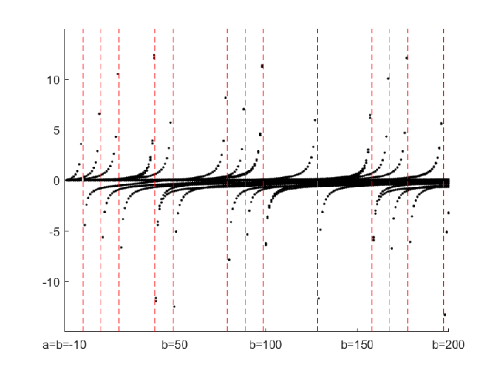
Refer to caption
Figure 2. Plot of the numerically calculated eigenvalues of Λ⁡(b)−Λ⁡(a)\Lambda(b)-\Lambda(a) (black dots) as a function of bb for fixed a:=−10a:=-10.

Let us stress however that this numerical experiment is only an indication of what might happen to stipulate further research. We do not have a rigorous proof that the observed drop in the number of negative eigenvalues really exists. Λ⁡(b)−Λ⁡(a)\Lambda(b)-\Lambda(a) is a compact operator with an infinite number of eigenvalues accumulating at zero, and we cannot rigorously rule out the possibility that there exist more negative eigenvalues (up to the theoretically proven bound d⁡(b)−d⁡(a)d(b)-d(a)) that we did not find due to their absolute values being below the numerical precision level.

References

  • [AH13] Lilian Arnold and Bastian Harrach. Unique shape detection in transient eddy current problems. Inverse Problems, 29(9):095004, 2013.
  • [BHHM17] Andrea Barth, Bastian Harrach, Nuutti Hyvönen, and Lauri Mustonen. Detecting stochastic inclusions in electrical impedance tomography. Inverse Problems, 33(11):115012, 2017.
  • [BHKS18] Tommi Brander, Bastian Harrach, Manas Kar, and Mikko Salo. Monotonicity and enclosure methods for the pp-Laplace equation. SIAM J. Appl. Math., 78(2):742–758, 2018.
  • [BS12] Feliks Aleksandrovich Berezin and M Shubin. The Schrödinger Equation, volume 66. Springer Science & Business Media, 2012.
  • [DS67] N. Dunford and J. T. Schwartz. Linear operators I–II. Interscience Publishers, 3rd printing, 1967.
  • [Gar17] Henrik Garde. Comparison of linear and non-linear monotononicity-based shape reconstruction using exact matrix characterizations. Inverse Problems in Science and Engineering, 2017.
  • [Geb08] Bastian Gebauer. Localized potentials in electrical impedance tomography. Inverse Probl. Imaging, 2(2):251–269, 2008.
  • [GH18] Roland Griesmaier and Bastian Harrach. Monotonicity in inverse medium scattering on unbounded domains. SIAM J. Appl. Math, 78(5):2533–2557, 2018.
  • [GM08] Fritz Gesztesy and Marius Mitrea. Generalized Robin boundary conditions, Robin-to-Dirichlet maps, and Krein-type resolvent formulas for Schrödinger operators on bounded Lipschitz domains. In Perspectives in partial differential equations, harmonic analysis and applications, volume 79 of Proc. Sympos. Pure Math., pages 105–173. Amer. Math. Soc., Providence, RI, 2008.
  • [GN13] Denis S Grebenkov and B-T Nguyen. Geometrical structure of laplacian eigenfunctions. SIAM Review, 55(4):601–667, 2013.
  • [GS17] Henrik Garde and Stratos Staboulis. Convergence and regularization for monotonicity-based shape reconstruction in electrical impedance tomography. Numerische Mathematik, 135(4):1221–1251, 2017.
  • [GS19] Henrik Garde and Stratos Staboulis. The regularized monotonicity method: Detecting irregular indefinite inclusions. Inverse Probl. Imaging, 13(1):93–116, 2019.
  • [Har09] Bastian Harrach. On uniqueness in diffuse optical tomography. Inverse Problems, 25:055010 (14pp), 2009.
  • [Har12] Bastian Harrach. Simultaneous determination of the diffusion and absorption coefficient from boundary data. Inverse Probl. Imaging, 6(4):663–679, 2012.
  • [Har19] Bastian Harrach. Uniqueness and Lipschitz stability in electrical impedance tomography with finitely many electrodes. Inverse Problems, 35(2):024005, 2019.
  • [HL18] Bastian Harrach and Yi-Hsuan Lin. Monotonicity-based inversion of the fractional Schrödinger equation I. Positive potentials. arXiv preprint arXiv:1711.05641, 2018.
  • [HL19] Bastian Harrach and Yi-Hsuan Lin. Monotonicity-based inversion of the fractional Schrödinger equation II. General potentials and stability. arXiv preprint arXiv:1903.08771, 2019.
  • [HLL18] Bastian Harrach, Yi-Hsuan Lin, and Hongyu Liu. On localizing and concentrating electromagnetic fields. SIAM J. Appl. Math, 78(5):2558–2574, 2018.
  • [HLU15] Bastian Harrach, Eunjung Lee, and Marcel Ullrich. Combining frequency-difference and ultrasound modulated electrical impedance tomography. Inverse Problems, 31(9):095003, 2015.
  • [HM16] Bastian Harrach and Mach Nguyet Minh. Enhancing residual-based techniques with shape reconstruction features in electrical impedance tomography. Inverse Problems, 32(12):125002, 2016.
  • [HM18] Bastian Harrach and Mach Nguyet Minh. Monotonicity-based regularization for phantom experiment data in electrical impedance tomography. In New Trends in Parameter Identification for Mathematical Models, pages 107–120. Springer, 2018.
  • [HM19] Bastian Harrach and Houcine Meftahi. Global uniqueness and Lipschitz-stability for the inverse Robin transmission problem. SIAM J. Appl. Math., 79(2):525–550, 2019.
  • [HPS] Bastian Harrach, Valter Pohjola, and Mikko Salo. Monotonicity and local uniqueness for the helmholtz equation. to appear in Anal. PDE.
  • [HS10] Bastian Harrach and Jin Keun Seo. Exact shape-reconstruction by one-step linearization in electrical impedance tomography. SIAM Journal on Mathematical Analysis, 42(4):1505–1518, 2010.
  • [HU13] Bastian Harrach and Marcel Ullrich. Monotonicity-based shape reconstruction in electrical impedance tomography. SIAM Journal on Mathematical Analysis, 45(6):3382–3403, 2013.
  • [HU15] Bastian Harrach and Marcel Ullrich. Resolution guarantees in electrical impedance tomography. IEEE Trans. Med. Imaging, 34:1513–1521, 2015.
  • [HU17] Bastian Harrach and Marcel Ullrich. Local uniqueness for an inverse boundary value problem with partial data. Proceedings of the American Mathematical Society, 145(3):1087–1095, 2017.
  • [HW08] G. H. Hardy and E. M. Wright. An introduction to the theory of numbers. Oxford University Press, Oxford, sixth edition, 2008.
  • [Kat95] Tosio Kato. Perturbation theory for linear operators. Classics in Mathematics. Springer-Verlag, Berlin, 1995.
  • [MVVT16] Antonio Maffucci, Antonio Vento, Salvatore Ventre, and Antonello Tamburrino. A novel technique for evaluating the effective permittivity of inhomogeneous interconnects based on the monotonicity property. IEEE Transactions on Components, Packaging and Manufacturing Technology, 6(9):1417–1427, 2016.
  • [Rem91] Reinhold Remmert. Theory of complex functions, volume 122 of Graduate Texts in Mathematics. Springer-Verlag, New York, 1991. Translated from the second German edition by Robert B. Burckel, Readings in Mathematics.
  • [RR04] Michael Renardy and Robert C. Rogers. An introduction to partial differential equations, volume 13 of Texts in Applied Mathematics. Springer-Verlag, New York, second edition, 2004.
  • [RS72] Michael Reed and Barry Simon. Methods of modern mathematical physics, Volume I: Functional analysis. Academic Press, San Diego, 1972.
  • [RS78] Michael Reed and Barry Simon. Methods of modern mathematical physics. IV. Analysis of operators. Academic Press, New York-London, 1978.
  • [SKJ+18] Jin Keun Seo, Kang Cheol Kim, Ariungerel Jargal, Kyounghun Lee, and Bastian Harrach. A learning-based method for solving ill-posed nonlinear inverse problems: a simulation study of lung eit. arXiv preprint arXiv:1810.10112, 2018.
  • [SUG+17] Zhiyi Su, Lalita Udpa, Gaspare Giovinco, Salvatore Ventre, and Antonello Tamburrino. Monotonicity principle in pulsed eddy current testing and its application to defect sizing. In Applied Computational Electromagnetics Society Symposium-Italy (ACES), 2017 International, pages 1–2. IEEE, 2017.
  • [TR02] Antonello Tamburrino and Guglielmo Rubinacci. A new non-iterative inversion method for electrical resistance tomography. Inverse Problems, 18(6):1809, 2002.
  • [TSV+16] Antonello Tamburrino, Zhiyi Sua, Salvatore Ventre, Lalita Udpa, and Satish S Udpa. Monotonicity based imang method in time domain eddy current testing. Electromagnetic Nondestructive Evaluation (XIX), 41:1, 2016.
  • [VMC+17] Salvatore Ventre, Antonio Maffucci, François Caire, Nechtan Le Lostec, Antea Perrotta, Guglielmo Rubinacci, Bernard Sartre, Antonio Vento, and Antonello Tamburrino. Design of a real-time eddy current tomography system. IEEE Transactions on Magnetics, 53(3):1–8, 2017.
  • [ZHS18] Liangdong Zhou, Bastian Harrach, and Jin Keun Seo. Monotonicity-based electrical impedance tomography for lung imaging. Inverse Problems, 34(4):045005, 2018.