跳到论文正文
W Papers独立论文阅读器 arXiv:1901.08353 论文正文 计算阅读时间 · 0%
引用这篇论文根据当前论文元数据生成,正式投稿前建议核对。


License: arXiv.org perpetual non-exclusive license
arXiv:1901.08353v1 [eess.SY] 24 Jan 2019

Stabilizing Scheduling Policies for Networked Control SystemsThanks: Atreyee Kundu is with the Department of Electrical Engineering, Indian Institute of Science Bangalore, India. Email: atreyeek@iisc.ac.in. Daniel E. Quevedo is with the Department of Electrical Engineering, Paderborn University, Germany. Email: dquevedo@ieee.org.

Atreyee Kundu and Daniel E. Quevedo
Date: August 11, 2026
Abstract.

This paper deals with the problem of allocating communication resources for Networked Control Systems (NCSs). We consider an NCS consisting of a set of discrete-time LTI plants whose stabilizing feedback loops are closed through a shared communication channel. Due to a limited communication capacity of the channel, not all plants can exchange information with their controllers at any instant of time. We propose a method to find periodic scheduling policies under which global asymptotic stability of each plant in the NCS is preserved. The individual plants are represented as switched systems, and the NCS is expressed as a weighted directed graph. We construct stabilizing scheduling policies by employing cycles on the underlying weighted directed graph of the NCS that satisfy appropriate contractivity conditions. We also discuss algorithmic design of these cycles.

Key words and phrases: 
networked control systems, scheduling policy, asymptotic stability, directed graphs, switched systems

1. Introduction

Networked Control Systems (NCSs) are omnipresent in modern day Cyber-Physical Systems (CPS) and Internet of Things (IoT) applications. While these applications typically involve a large-scale setting, the network resources are often limited. Consequently, multiple plants may need to share a communication channel (or network) for exchanging information with their remotely located controllers. Examples of communication networks with limited bandwidth include wireless networks (an important component of smart home, smart transportation, smart city, remote surgery, platoons of autonomous vehicles, etc.) and underwater acoustic communication systems. The often encountered scenario wherein the number of plants sharing a communication channel is higher than the capacity of the channel is called medium access constraint.

In this paper we consider an NCS consisting of multiple discrete-time linear plants whose feedback loops are closed through a shared communication channel. A block diagram of such an NCS is shown in Figure 1.

Controller 1Plant 1Controller 2Plant 2Controller NPlant NCommunication channel⋮\vdots
Figure 1. Block diagram of NCS

We assume that the plants are unstable in open-loop and asymptotically stable in closed-loop. Due to a limited communication capacity of the channel, only a few plants can exchange information with their controllers at any instant of time. Consequently, the remaining plants operate in open-loop at every time instant. Our objective is to allocate the shared communication channel to the set of plants in a manner so that stability of all plants is preserved. This task of efficient allocation of communication resources is commonly referred to as a scheduling problem, and the corresponding allocation scheme is called a scheduling policy.

Scheduling policies that preserve qualitative behaviour of an NCS under limited communication and/or computation resources are widely researched upon, and tools from both control theory and communication theory have been explored, see the recent works [30, 1, 28, 8, 23] and the references therein. These policies can be broadly classified into two categories: static (also called periodic, fixed, or open-loop) and dynamic (also called non-periodic, or closed-loop) scheduling. In case of the former, a finite length allocation scheme of the shared communication channel is determined offline and is applied eternally in a periodic manner, while in case of the latter, the allocation is determined based on some information (e.g., states, outputs, access status of sensors and actuators, etc.) about the plant. In this paper we will focus on periodic scheduling policies that preserve global asymptotic stability (GAS) of all plants in an NCS. We will call such scheduling policies as stabilizing scheduling policies. Static scheduling policies are easier to implement, often near optimal, and guarantee activation of each sensor and actuator, see [26, 22, 12] for detailed discussions. They are preferred for safety-critical control systems [22, §2.5.1]. It is also observed in [25, 26] that periodic phenomenon appears in non-periodic schedules.

For NCSs with continuous-time linear plants, stabilizing periodic scheduling policies are characterized using common Lyapunov functions [9] and piecewise Lyapunov-like functions with average dwell time switching [21]. A more general case of co-designing a static scheduling policy and control action is addressed using combinatorial optimization with periodic control theory in [27] and Linear Matrix Inequalities (LMIs) optimization with average dwell time technique in [5]. In the discrete-time setting, the authors of [31] characterize periodic switching sequences that ensure reachability and observability of the plants under limited communication, and design an observer-based feedback controller for these periodic sequences. The techniques were later extended to the case of constant transmission delays [10] and Linear Quadratic Gaussian (LQG) control problem [11]. Periodic sensor scheduling schemes that accommodate limited communication and adversary attacks are studied recently in [29].

The main contribution of this paper lies in combining switched systems and graph theory to propose a new class of stabilizing scheduling policies for NCSs. We represent the individual (open-loop unstable) plants of an NCS as switched systems, where the switching is between their open-loop (unstable mode) and closed-loop (stable mode) operations. Clearly, within our setting, no switched system can operate in stable mode for all time as that will destabilize some of the plants in the NCS. The search for a stabilizing scheduling policy then becomes the problem of finding switching logics that obey the limitations of the shared channel and preserve stability. It is assumed that the exchange of information between a plant and its controller is not affected by communication uncertainties. In the recent past, graph theoretic techniques have played an important role in designing stabilizing switching logics for switched systems, see e.g., [16, 15] and the references therein. In the present work we associate a weighted directed graph with the NCS that captures the communication limitation of the shared channel, and design stabilizing switching logics for each plant in the NCS. Multiple Lyapunov-like functions are employed for analyzing stability of the switched systems. The stabilizing switching logics form a stabilizing scheduling policy. The switching logics are combined in terms of a class of cycles on the underlying weighted directed graph of the NCS that satisfies appropriate contractivity properties. We also discuss algorithmic construction of these cycles.

In brief, our contributions are:

  • ∘\circ

    Given an NCS with discrete-time linear plants that exchange information with their stabilizing controllers through a shared channel of limited communication capacity, we present an algorithm to design a scheduling policy that preserves GAS of each plant in the NCS. Our scheduling policy is periodic in nature, and relies on the existence of what we call a TT-contractive cycle on the underlying weighted directed graph of the NCS. Periodic scheduling policies are proven to be immensely useful in process control, where many loops need to share a common communication resource as it avoids the necessity of frequent network reconfigurations. In fact, periodic scheduling is an inherent feature of IEEE 802.15.4 networks [26] which underlie commercial standards, such as WirelessHart, ISA100.11a and ZigBee. The use of cycles on a weighted directed graph makes our techniques numerically tractable, see Remark 11 for a detailed discussion.

  • ∘\circ

    We address algorithmic design of TT-contractive cycles. Given the connectivity of the underlying weighted directed graph of the NCS and description of the individual plants, we fix a cycle on this graph and present an algorithm that designs multiple Lyapunov-like functions such that the above cycle is TT-contractive. We also identify sufficient conditions on the multiple Lyapunov-like functions and channel constraints under which the existence of a TT-contractive cycle is guaranteed.

The remainder of this paper is organized as follows: in §2 we formulate the problem under consideration, and describe the primary apparatus for our analysis. Our method for constructing stabilizing periodic scheduling policies appears in §3. In §4 we discuss algorithmic design of TT-contractive cycles. Numerical examples are presented in §5 to demonstrate our results. We conclude in §6 with a brief discussion of future research directions. A proof of our main Theorem appears in §7.

Some notation used in this paper: ℕ={1,2,…}\mathbb{N}=\{1,2,\ldots\} is the set of natural numbers, ℕ0={0}∪ℕ\mathbb{N}_{0}=\{0\}\cup\mathbb{N}, and ℝ\mathbb{R} is the set of real numbers. We let ]k1:k2]]k_{1}:k_{2}] denote the set {n∈ℕ|k1<n≤k2}\{n\in\mathbb{N}\>|\>k_{1}<n\leq k_{2}\}. For a scalar mm, let |m|\left\lvert{m}\right\rvert denote its absolute value, and for a set MM, let |M|\left\lvert{M}\right\rvert denote its cardinality. Let ‖⋅‖\left\lVert\cdot\right\rVert be the standard 22-norm and ⊤ denote the transpose operation.

2. Preliminaries

We consider an NCS with NN discrete-time linear plants. Each plant communicates with its remotely located controller through a shared communication channel, see Figure 1. The plant dynamics are

(1) xi(t+1)=Aixi(t)+Biui(t),xi(0)=xi0,i=1,2,…,N,t∈ℕ0,\displaystyle x_{i}(t+1)=A_{i}x_{i}(t)+B_{i}u_{i}(t),\>x_{i}(0)=x_{i}^{0},\>i=1,2,\ldots,N,\>t\in\mathbb{N}_{0},

where xi​(t)∈ℝdx_{i}(t)\in\mathbb{R}^{d} and ui​(t)∈ℝmu_{i}(t)\in\mathbb{R}^{m} are the vectors of states and inputs of the ii-th plant at time tt, respectively. Each plant ii employs a state-feedback controller given by ui​(t)=Ki​xi​(t)u_{i}(t)=K_{i}x_{i}(t), i=1,2,…,Ni=1,2,\ldots,N. The matrices Ai∈ℝd×dA_{i}\in\mathbb{R}^{d\times d}, Bi∈ℝd×mB_{i}\in\mathbb{R}^{d\times m} and Ki∈ℝm×dK_{i}\in\mathbb{R}^{m\times d}, i=1,2,…,Ni=1,2,\ldots,N are known. The shared channel has a limited communication capacity: at any time instant, only MM plants (0<M<N0<M<N) can access the channel. Consequently, N−MN-M plants operate in open loop at every time instant. We define

𝒮:={s∈{1,2,…,N}M|all elements of​s​are distinct}\mathcal{S}:=\{s\in\{1,2,\ldots,N\}^{M}\>|\>\>\text{all elements of}\>\>s\>\>\text{are distinct}\}

to be the set of vectors that consist of MM distinct elements from {1,2,…,N}\{1,2,\ldots,N\}. We call a function γ:ℕ0→𝒮\gamma:\mathbb{N}_{0}\to\mathcal{S} a scheduling policy. There exists a diverging sequence of times 0=:τ0<τ1<τ2<⋯0=:\tau_{0}<\tau_{1}<\tau_{2}<\cdots and a sequence of indices s0,s1,s2,…s_{0},s_{1},s_{2},\ldots with sj∈𝒮s_{j}\in\mathcal{S}, j=0,1,2,…j=0,1,2,\ldots such that γ⁡(t)=sj\gamma(t)=s_{j} for t∈[τj:τj+1[t\in[\tau_{j}:\tau_{j+1}[, j=0,1,2,…j=0,1,2,\ldots. The role of γ\gamma is to specify, at every time tt, MM plants of the NCS which access the communication channel at that time. The remaining N−MN-M plants operate in open loop, in particular, with ui​(t)=0u_{i}(t)=0.

Remark 1.

One may also study a scheduling problem in the setting of the remaining N−MN-M plants operating with ui​(t)=u¯u_{i}(t)=\overline{u}, where u¯\overline{u} is the last control input received before time tt. However, in this paper we consider open-loop evolution of a plant whenever it is not accessing the shared communication channel.

We will work under the following set of assumptions:

Assumption 1.

The open-loop dynamics of each plant is unstable and each controller is stabilizing. More specifically, the matrices Ai+Bi​KiA_{i}+B_{i}K_{i}, i=1,2,…,Ni=1,2,\ldots,N are Schur stable and the matrices AiA_{i}, i=1,2,…,Ni=1,2,\ldots,N are unstable.11 1 We call a matrix unstable, if it is not Schur stable.

Assumption 2.

The shared communication channel is ideal in the sense that exchange of information between plants and their controllers is not affected by communication uncertainties.

In view of Assumption 1, each plant in (1) operates in two modes: stable mode when the plant has access to the shared communication channel and unstable mode when the plant does not have access to the channel. Let us denote the stable and unstable modes of the ii-th plant as isi_{s} and iui_{u}, respectively, Ais=Ai+Bi​KiA_{i_{s}}=A_{i}+B_{i}K_{i} and Aiu=AiA_{i_{u}}=A_{i}, i=1,2,…,Ni=1,2,\ldots,N. In this paper we are interested in a scheduling policy that guarantees GAS of each plant in (1). In particular, we study the following problem:

Problem 1.

Given the matrices AiA_{i}, BiB_{i}, KiK_{i}, i=1,2,…,Ni=1,2,\ldots,N, and a number M(<N)M(<N), find a scheduling policy that ensures global asymptotic stability (GAS) of each plant ii in (1).

We will call a scheduling policy γ\gamma that is a solution to Problem 1, as a stabilizing scheduling policy. Recall that

Definition 1 ([14, Lemma 4.4]).

The ii-th plant in (1) is GAS for a given scheduling policy γ\gamma, if there exists a class 𝒦​ℒ\mathcal{KL} function βi\beta_{i} such that the following inequality holds:

(2) ‖xi​(t)‖≤βi​(‖xi​(0)‖,t)​for all​xi​(0)∈ℝd​and​t≥0.\displaystyle\left\lVert x_{i}(t)\right\rVert\leq\beta_{i}(\left\lVert x_{i}(0)\right\rVert,t)\>\>\text{for all}\>x_{i}(0)\in\mathbb{R}^{d}\>\>\text{and}\>\>t\geq 0.

Towards solving Problem 1, we express individual plants in (1) as switched systems and associate a weighted directed graph with the NCS under consideration. Our solution to Problem 1 involves two steps:

  • ∘\circ

    first, we present an algorithm that constructs a scheduling policy by employing what we call a TT-contractive cycle on the underlying weighted directed graph of the NCS, and

  • ∘\circ

    second, we show that a scheduling policy obtained from our algorithm ensures GAS of each plant in (1).

We also discuss algorithmic design of TT-contractive cycles. In the remainder of this section we catalog our analysis tools.

2.1. Individual plants and switched systems

The dynamics of the ii-th plant in (1) can be expressed as a switched system [20, §1.1.2]

(3) xi​(t+1)=Aσi​(t)​xi​(t),xi​(0)=xi0,σi​(t)∈{is,iu},t∈ℕ0,\displaystyle x_{i}(t+1)=A_{\sigma_{i}(t)}x_{i}(t),\>\>x_{i}(0)=x_{i}^{0},\>\sigma_{i}(t)\in\{i_{s},i_{u}\},\>t\in\mathbb{N}_{0},

where the subsystems are {Ais,Aiu}\{A_{i_{s}},A_{i_{u}}\} and a switching logic σi:ℕ0→{is,iu}\sigma_{i}:\mathbb{N}_{0}\to\{i_{s},i_{u}\} satisfies:

σi​(t)={is,if​i​is an element of​γ​(t),iu,otherwise.\sigma_{i}(t)=\begin{cases}i_{s},\>\>&\text{if}\>\>i\>\>\text{is an element of}\>\>\gamma(t),\\ i_{u},\>\>&\text{otherwise}.\end{cases}

Clearly, a switching logic σi\sigma_{i}, i=1,2,…,Ni=1,2,\ldots,N is a function of the scheduling policy γ\gamma. In order to ensure GAS of the individual plants, it therefore, suffices to look for a γ\gamma that renders each σi\sigma_{i} stabilizing in the following sense: σi\sigma_{i} guarantees GAS of switched system (3) for each i=1,2,…,Ni=1,2,\ldots,N. We recall the following facts from recent literature:

Fact 1.

[16, Fact 1] For each i=1,2,…,Ni=1,2,\ldots,N, there exist pairs (Pp,λp)(P_{p},\lambda_{p}), p∈{is,iu}p\in\{i_{s},i_{u}\}, where Pp∈ℝd×dP_{p}\in\mathbb{R}^{d\times d} are symmetric and positive definite matrices, and 0<λis<10<\lambda_{i_{s}}<1, λiu≥1\lambda_{i_{u}}\geq 1, such that with

(4) ℝd∋ξ⟼Vp(ξ):=⟨Ppξ,ξ⟩∈[0,+∞[,\displaystyle\mathbb{R}^{d}\ni\xi\longmapsto V_{p}(\xi):=\langle P_{p}\xi,\xi\rangle\in[0,+\infty[,

we have

(5) Vp​(zp​(t+1))≤λp​Vp​(zp​(t)),t∈ℕ0,\displaystyle V_{p}(z_{p}(t+1))\leq\lambda_{p}V_{p}(z_{p}(t)),\>\>t\in\mathbb{N}_{0},

and zp​(⋅)z_{p}(\cdot) solves the pp-th recursion in (3), p∈{is,iu}p\in\{i_{s},i_{u}\}.

Fact 2.

[16, Fact 2] For each i=1,2,…,Ni=1,2,\ldots,N, there exist μp​q≥1\mu_{pq}\geq 1 such that

(6) Vq​(ξ)≤μp​q​Vp​(ξ)​for all​ξ∈ℝd​and​p,q∈{is,iu}.\displaystyle V_{q}(\xi)\leq\mu_{pq}V_{p}(\xi)\>\>\text{for all}\>\>\xi\in\mathbb{R}^{d}\>\>\text{and}\>\>p,q\in\{i_{s},i_{u}\}.

The functions VpV_{p}, p∈{is,iu}p\in\{i_{s},i_{u}\}, i=1,2,…,Ni=1,2,\ldots,N are called Lyapunov-like functions, and they are widely used in stability theory of switched and hybrid systems [4, 20]. We will use properties of these functions described in Facts 1 and 2, in our analysis towards deriving a stabilizing scheduling policy. The scalars λp\lambda_{p}, p∈{is,iu}p\in\{i_{s},i_{u}\} give quantitative measures of (in)stability associated to (un)stable modes of operation of the ii-th plant. Linear comparability of VpV_{p}’s in (6) follows from the definition of VpV_{p}, p∈{is,iu}p\in\{i_{s},i_{u}\} in (4). In [16, Proposition 1] a tight estimate of the scalars μp​q\mu_{pq}, p,q∈{is,iu}p,q\in\{i_{s},i_{u}\} was proposed to be λmax​(Pq​Pp−1)\lambda_{\max}(P_{q}P_{p}^{-1}), where λmax​(M)\lambda_{\max}(M) denotes the maximum eigenvalue of a matrix M∈ℝd×dM\in\mathbb{R}^{d\times d}.

2.2. NCS and directed graphs

Recall that a directed graph is a set of vertices connected by edges, where each edge has a direction associated to it. We connect a directed graph 𝒢⁡(𝒱,ℰ)\mathcal{G}(\mathcal{V},\mathcal{E}) with the NCS under consideration. 𝒢⁡(𝒱,ℰ)\mathcal{G}(\mathcal{V},\mathcal{E}) contains:

  • ∘\circ

    a vertex set 𝒱\mathcal{V} consisting of (NM)N\choose M vertices that are labelled distinctly. The label associated to a vertex vv is given by L⁡(v)={ℓv​(1),ℓv​(2),…,ℓv​(N)}L(v)=\{\ell_{v}(1),\ell_{v}(2),\ldots,\ell_{v}(N)\}, where ℓv​(i)=is\ell_{v}(i)=i_{s} for any MM elements and ℓv​(i)=iu\ell_{v}(i)=i_{u} for the remaining N−MN-M elements. Two labels L⁡(u)L(u) and L⁡(v)L(v) are equal if ℓu​(i)=ℓv​(i)\ell_{u}(i)=\ell_{v}(i) for all i=1,2,…,Ni=1,2,\ldots,N. By the term distinct labelling, we mean that L⁡(u)=L⁡(v)L(u)=L(v) whenever u=v∈𝒱u=v\in\mathcal{V}.

  • ∘\circ

    an edge set ℰ\mathcal{E} consisting of a directed edge (u,v)(u,v) from every vertex u∈𝒱u\in\mathcal{V} to every vertex v∈𝒱v\in\mathcal{V}, v≠uv\neq u.

The label L⁡(v)L(v) corresponding to a vertex v∈𝒱v\in\mathcal{V} gives a combination of MM plants operating in stable mode and the remaining N−MN-M plants operating in unstable mode. Since 𝒱\mathcal{V} contains (NM)N\choose M vertices and the label associated to each vertex is distinct, it follows that the set of vertex labels consists of all possible combinations of MM plants accessing the communication channel and N−MN-M plants operating in open-loop. A directed edge (u,v)(u,v) from a vertex uu to a vertex v(≠u)v\>(\neq u) corresponds to a transition from a set of MM plants accessing the communication channel (as specified by L⁡(u)L(u)) to another set of MM plants accessing the communication channel (as specified by L⁡(v)L(v)). In the sequel we may abbreviate 𝒢⁡(𝒱,ℰ)\mathcal{G}(\mathcal{V},\mathcal{E}) as 𝒢\mathcal{G} if there is no risk of confusion.

We use functions w¯:𝒱→ℝN\overline{w}:\mathcal{V}\to\mathbb{R}^{N} and w¯:ℰ→ℝN\underline{w}:\mathcal{E}\to\mathbb{R}^{N} to associate weights to the vertices and edges of 𝒢\mathcal{G}, respectively. They are defined as

w¯​(v)\displaystyle\overline{w}(v) =(w¯1​(v)w¯2​(v)w¯N​(v)),v∈𝒱,where\displaystyle=\begin{pmatrix}\overline{w}_{1}(v)\\ \overline{w}_{2}(v)\\ \vdots\\ \overline{w}_{N}(v)\end{pmatrix},\>\>v\in\mathcal{V},\>\>\text{where}
(7) w¯i​(v)\displaystyle\overline{w}_{i}(v) ={−|ln⁡λis|,if​ℓv​(i)=is,|ln⁡λiu|,if​ℓv​(i)=iu,i=1,2,…,N,\displaystyle=\begin{cases}-\left\lvert{\ln\lambda_{i_{s}}}\right\rvert,\>\>\>\>&\text{if}\>\>\ell_{v}(i)=i_{s},\\ \left\lvert{\ln\lambda_{i_{u}}}\right\rvert,\>\>\>\>&\text{if}\>\>\ell_{v}(i)=i_{u},\end{cases}\quad i=1,2,\ldots,N,
and
w¯​(u,v)\displaystyle\underline{w}(u,v) =(w¯1​(u,v)w¯2​(u,v)w¯N​(u,v)),(u,v)∈ℰ,where\displaystyle=\begin{pmatrix}\underline{w}_{1}(u,v)\\ \underline{w}_{2}(u,v)\\ \vdots\\ \underline{w}_{N}(u,v)\end{pmatrix},\>\>(u,v)\in\mathcal{E},\>\>\text{where}
(8) w¯i​(u,v)\displaystyle\underline{w}_{i}(u,v) ={ln⁡μis​iu,if​ℓu​(i)=is​and​ℓv​(i)=iu,ln⁡μiu​is,if​ℓu​(i)=iu​and​ℓv​(i)=is,0,otherwise,​i=1,2,…,N.\displaystyle=\begin{cases}\ln\mu_{i_{s}i_{u}},&\text{if}\>\>\ell_{u}(i)=i_{s}\>\text{and}\>\ell_{v}(i)=i_{u},\\ \ln\mu_{i_{u}i_{s}},&\text{if}\>\>\ell_{u}(i)=i_{u}\>\text{and}\>\ell_{v}(i)=i_{s},\\ 0,\>\>\>\>&\text{otherwise},\end{cases}\>\>i=1,2,\ldots,N.

Here λis\lambda_{i_{s}}, λiu\lambda_{i_{u}}, and μis​iu\mu_{i_{s}i_{u}}, μiu​is\mu_{i_{u}i_{s}}, i=1,2,…,Ni=1,2,\ldots,N are as described in Facts 1 and 2, respectively.

Remark 2.

We will aim for achieving GAS of each switched system (3), i=1,2,…,Ni=1,2,\ldots,N. For this purpose, we will compensate the increase in VpV_{p}, p∈{is,iu}p\in\{i_{s},i_{u}\} caused by activation of unstable mode iui_{u} and switches between stable and unstable modes (isi_{s} to iui_{u} and iui_{u} to isi_{s}) by the decrease in VpV_{p}, p∈{is,iu}p\in\{i_{s},i_{u}\} achieved by using the stable modes isi_{s}, i=1,2,…,Ni=1,2,\ldots,N. As a natural choice, the vertex (subsystem) weights of 𝒢\mathcal{G} relate to the rate of increase/decrease of the Lyapunov-like functions VpV_{p} captured by the scalars λp\lambda_{p}, p∈{is,iu}p\in\{i_{s},i_{u}\}, and the edge (switch) weights of 𝒢\mathcal{G} relate to the “jump” between Lyapunov-like functions VpV_{p} and VqV_{q}, p,q∈{is,iu}p,q\in\{i_{s},i_{u}\} captured by the scalars μp​q\mu_{pq}, p,q∈{is,iu}p,q\in\{i_{s},i_{u}\}, i=1,2,…,Ni=1,2,\ldots,N.33 3 The use of absolute value and natural logarithm is explained in context, see Remark 15.

Example 1.

Consider an NCS with N=3N=3 and M=2M=2. The corresponding directed graph 𝒢\mathcal{G} has

  • ∘\circ

    (32)=3{3\choose 2}=3 vertices, 𝒱={v¯1,v¯2,v¯3}\mathcal{V}=\{\overline{v}_{1},\overline{v}_{2},\overline{v}_{3}\} with labels L⁡(v¯1)={1s,2s,3u}L(\overline{v}_{1})=\{1_{s},2_{s},3_{u}\}, L⁡(v¯2)={1s,2u,3s}L(\overline{v}_{2})=\{1_{s},2_{u},3_{s}\}, L⁡(v¯3)={1u,2s,3s}L(\overline{v}_{3})=\{1_{u},2_{s},3_{s}\}, and

  • ∘\circ

    66 directed edges, ℰ={(v¯1,v¯2),(v¯1,v¯3),(v¯2,v¯1),(v¯2,v¯3)\mathcal{E}=\{(\overline{v}_{1},\overline{v}_{2}),(\overline{v}_{1},\overline{v}_{3}),(\overline{v}_{2},\overline{v}_{1}),(\overline{v}_{2},\overline{v}_{3}),(v¯3,v¯1),(v¯3,v¯2)}(\overline{v}_{3},\overline{v}_{1}),(\overline{v}_{3},\overline{v}_{2})\}.

A pictorial representation of 𝒢\mathcal{G} is shown below.

v¯1\overline{v}_{1} v¯2\overline{v}_{2} v¯3\overline{v}_{3}

The weights associated to the vertices and edges of 𝒢\mathcal{G} are:

w¯​(v¯1)=(−|ln⁡λ1s|−|ln⁡λ2s||ln⁡λ3u|),\displaystyle\overline{w}(\overline{v}_{1})=\begin{pmatrix}-\left\lvert{\ln\lambda_{1_{s}}}\right\rvert\\ -\left\lvert{\ln\lambda_{2_{s}}}\right\rvert\\ \left\lvert{\ln\lambda_{3_{u}}}\right\rvert\end{pmatrix},\>\> w¯​(v¯2)=(−|ln⁡λ1s||ln⁡λ2u|−|ln⁡λ3s|),w¯​(v¯3)=(|ln⁡λ1u|−|ln⁡λ2s|−|ln⁡λ3s|),\displaystyle\>\>\overline{w}(\overline{v}_{2})=\begin{pmatrix}-\left\lvert{\ln\lambda_{1_{s}}}\right\rvert\\ \left\lvert{\ln\lambda_{2_{u}}}\right\rvert\\ -\left\lvert{\ln\lambda_{3_{s}}}\right\rvert\end{pmatrix},\>\>\overline{w}(\overline{v}_{3})=\begin{pmatrix}\left\lvert{\ln\lambda_{1_{u}}}\right\rvert\\ -\left\lvert{\ln\lambda_{2_{s}}}\right\rvert\\ -\left\lvert{\ln\lambda_{3_{s}}}\right\rvert\end{pmatrix},
and
w¯​(v¯1,v¯2)=(0ln⁡μ2s​2uln⁡μ3u​3s),\displaystyle\underline{w}(\overline{v}_{1},\overline{v}_{2})=\begin{pmatrix}0\\ \ln\mu_{2_{s}2_{u}}\\ \ln\mu_{3_{u}3_{s}}\end{pmatrix},\>\> w¯​(v¯1,v¯3)=(ln⁡μ1s​1u0ln⁡μ3u​3s),w¯​(v¯2,v¯1)=(0ln⁡μ2u​2sln⁡μ3s​3u),\displaystyle\>\>\underline{w}(\overline{v}_{1},\overline{v}_{3})=\begin{pmatrix}\ln\mu_{1_{s}1_{u}}\\ 0\\ \ln\mu_{3_{u}3_{s}}\end{pmatrix},\underline{w}(\overline{v}_{2},\overline{v}_{1})=\begin{pmatrix}0\\ \ln\mu_{2_{u}2_{s}}\\ \ln\mu_{3_{s}3_{u}}\end{pmatrix},
w¯​(v¯2,v¯3)=(ln⁡μ1s​1uln⁡μ2u​2s0),\displaystyle\underline{w}(\overline{v}_{2},\overline{v}_{3})=\begin{pmatrix}\ln\mu_{1_{s}1_{u}}\\ \ln\mu_{2_{u}2_{s}}\\ 0\end{pmatrix},\>\> w¯​(v¯3,v¯1)=(ln⁡μ1u​1s0ln⁡μ3s​3u),w¯​(v¯3,v¯2)=(ln⁡μ1u​1sln⁡μ2s​2u0).\displaystyle\>\>\underline{w}(\overline{v}_{3},\overline{v}_{1})=\begin{pmatrix}\ln\mu_{1_{u}1_{s}}\\ 0\\ \ln\mu_{3_{s}3_{u}}\end{pmatrix},\underline{w}(\overline{v}_{3},\overline{v}_{2})=\begin{pmatrix}\ln\mu_{1_{u}1_{s}}\\ \ln\mu_{2_{s}2_{u}}\\ 0\end{pmatrix}.
Remark 3.

By construction of 𝒢\mathcal{G}, it contains two directed edges (u,v)(u,v) and (v,u)(v,u) between every two vertices u,v∈𝒱u,v\in\mathcal{V}. Employing an undirected graph instead of a directed one may appear to be a natural choice here. However, the use of directed edges allows us to distinguish easily between the transitions isi_{s} to iui_{u} and iui_{u} to isi_{s}, i=1,2,…,Ni=1,2,\ldots,N, and assign weights to the corresponding edges accordingly. Notice that since the vertex labels are distinct, for every two vertices u,v∈𝒱u,v\in\mathcal{V}, there exists at least one ii for which w¯i​(u,v)\underline{w}_{i}(u,v) and w¯i​(v,u)\underline{w}_{i}(v,u) are different, i∈{1,2,…,N}i\in\{1,2,\ldots,N\}.

Recall that [3, p. 4] a walk on a directed graph G⁡(V,E)G(V,E) is an alternating sequence of vertices and edges W=v~0,e~1,v~1,e~2W=\tilde{v}_{0},\tilde{e}_{1},\tilde{v}_{1},\tilde{e}_{2},v~2\tilde{v}_{2},
…,v~ℓ−1,e~ℓ,v~ℓ\ldots,\tilde{v}_{\ell-1},\tilde{e}_{\ell},\tilde{v}_{\ell}, where v~m∈V\tilde{v}_{m}\in V, e~m=(v~m−1,v~m)∈E\tilde{e}_{m}=(\tilde{v}_{m-1},\tilde{v}_{m})\in E, 0<m≤ℓ0<m\leq\ell. The length of a walk is its number of edges, counting repetitions, e.g., the length of WW is ℓ\ell. The initial vertex of WW is v~0\tilde{v}_{0} and the final vertex of WW is v~ℓ\tilde{v}_{\ell}. If v~ℓ=v~0\tilde{v}_{\ell}=\tilde{v}_{0}, we say that the walk is closed. A closed walk is called a cycle if the vertices v~k\tilde{v}_{k}, 0<k<n0<k<n are distinct from each other and v~0\tilde{v}_{0}. We will use the following class of cycles on 𝒢\mathcal{G} for constructing a stabilizing scheduling policy:

Definition 2.

A cycle W=v0,(v0,v1),v1,⋯,vn−1,(vn−1,v0)W=v_{0},(v_{0},v_{1}),v_{1},\cdots,v_{n-1},(v_{n-1},v_{0}),v0v_{0} on 𝒢⁡(𝒱,ℰ)\mathcal{G}(\mathcal{V},\mathcal{E}) is called TT-contractive if there exist integers Tvj>0T_{v_{j}}>0, j=0,1,…,n−1j=0,1,\ldots,n-1, 2≤n≤|𝒱|2\leq n\leq\left\lvert{\mathcal{V}}\right\rvert such that the following set of inequalities is satisfied:

(9) Ξi(W):=∑j=0n−1w¯i(vj)Tvj+∑j=0vn:=v0n−1w¯i(vj,vj+1)<0\displaystyle\Xi_{i}(W):=\sum_{j=0}^{n-1}\overline{w}_{i}(v_{j})T_{v_{j}}+\sum_{\begin{subarray}{c}j=0\\ v_{n}:=v_{0}\end{subarray}}^{n-1}\underline{w}_{i}(v_{j},v_{j+1})<0

for all i=1,2,…,Ni=1,2,\ldots,N, where nn is the length of WW, w¯​(vj)\overline{w}(v_{j}) is the weight associated to vertex vjv_{j}, w¯i​(vj)\overline{w}_{i}(v_{j}) is the ii-th element of w¯​(vj)\overline{w}(v_{j}), and w¯​(vj,vj+1)\underline{w}(v_{j},v_{j+1}) is the weight associated to edge (vj,vj+1)(v_{j},v_{j+1}), w¯i​(vj,vj+1)\underline{w}_{i}(v_{j},v_{j+1}) is the ii-th element of w¯​(vj,vj+1)\underline{w}(v_{j},v_{j+1}), i=1,2,…,Ni=1,2,\ldots,N, j=0,1,…,n−1j=0,1,\ldots,n-1. We call the scalar TvjT_{v_{j}} as the TT-factor of vertex vjv_{j}, j=0,1,…,n−1j=0,1,\ldots,n-1.

We will employ the integers TvjT_{v_{j}}, j=0,1,…,n−1j=0,1,\ldots,n-1 to associate a time duration with every vertex vjv_{j}, j=0,1,…,n−1j=0,1,\ldots,n-1 that appears in WW. This time duration will determine how long a set of MM plants can access the shared communication channel while preserving GAS of all plants in the NCS under consideration. In the present discrete-time setting, the association of integers with time durations is natural.

Remark 4.

Definition 2 is an extension of [15, Definition 2] to a set of NN switched systems in the discrete-time setting. In [15] the notion of a contractive cycle with TT-factors chosen from a given interval of real numbers was used to study input/output-to-state stability (IOSS) of continuous-time switched nonlinear systems under dwell time restrictions.

Example 2.

Consider the setting of Example 1. Suppose that

λ1s=λ2s=λ3s=0.25,\displaystyle\lambda_{1_{s}}=\lambda_{2_{s}}=\lambda_{3_{s}}=0.25,\>\> λ1u=λ2u=λ3u=1.1,\displaystyle\>\>\lambda_{1_{u}}=\lambda_{2_{u}}=\lambda_{3_{u}}=1.1,
μ1s​1u=μ2s​2u=μ3s​3u=1.1,\displaystyle\mu_{1_{s}1_{u}}=\mu_{2_{s}2_{u}}=\mu_{3_{s}3_{u}}=1.1,\>\> μ1u​1s=μ2u​2s=μ3u​3s=1.2.\displaystyle\>\>\mu_{1_{u}1_{s}}=\mu_{2_{u}2_{s}}=\mu_{3_{u}3_{s}}=1.2.

The cycle W=1,(1,2),2,(2,1),1W=1,(1,2),2,(2,1),1 on 𝒢\mathcal{G} is TT-contractive with TT-factors T1=5T_{1}=5 and T2=4T_{2}=4. Indeed, Ξ1​(W)=−1.3863\Xi_{1}(W)=-1.3863, Ξ2​(W)=−6.2726\Xi_{2}(W)=-6.2726 and Ξ3​(W)=−4.791\Xi_{3}(W)=-4.791.

We are now in a position to describe our solution to Problem 1.

3. Stabilizing periodic scheduling policies

The following algorithm is geared towards constructing a periodic scheduling policy. We will show that a scheduling policy obtained from this algorithm is stabilizing. Let 𝒢⁡(𝒱,ℰ)\mathcal{G}(\mathcal{V},\mathcal{E}) be a directed graph representation of the NCS described in §2.Suppose that 𝒢⁡(𝒱,ℰ)\mathcal{G}(\mathcal{V},\mathcal{E}) admits a TT-contractive cycle W=v0,(v0,v1),v1,…,vn−1,(vn−1,v0),v0W=v_{0},(v_{0},v_{1}),v_{1},\ldots,v_{n-1},(v_{n-1},v_{0}),v_{0} (of length nn) with TT-factors T0T_{0}, T1,…T_{1},\ldots, Tn−1T_{n-1}.

Algorithm 1 Construction of a periodic scheduling policy
0:  a TT-contractive cycle W=v0,(v0,v1),v1,…,vn−1W=v_{0},(v_{0},v_{1}),v_{1},\ldots,v_{n-1},(vn−1,v0),v0(v_{n-1},v_{0}),v_{0} and corresponding TT-factors T0,T1,…,Tn−1T_{0},T_{1},\ldots,T_{n-1}
0:  a periodic scheduling policy γ\gamma Step I: For each vertex vjv_{j}, j=0,1,…,n−1j=0,1,\ldots,n-1, pick the elements ii with label ℓvj​(i)=is\ell_{v_{j}}(i)=i_{s}, i=1,2,…,Ni=1,2,\ldots,N, and construct MM- dimensional vectors sjs_{j}, j=0,1j=0,1,…,n−1\ldots,n-1.
1:  for j=0,1,…,n−1j=0,1,\ldots,n-1 do
2:   Set p=0p=0
3:   for i=1,2,…,Ni=1,2,\ldots,N do
4:    if ℓvj​(i)=is\ell_{v_{j}}(i)=i_{s} then
5:     Set p=p+1p=p+1 and sj​(p)=i{s_{j}(p)}=i
6:    end if
7:   end for
8:  end forStep II: Construct a scheduling policy using the vectors sjs_{j},j=0,1,…,n−1j=0,1,\ldots,n-1 obtained in Step I and the TT-factors TvjT_{v_{j}},j=0,1,…,n−1j=0,1,\ldots,n-1
9:  Set p=0p=0 and τ0=0\tau_{0}=0
10:  for q=p​n,p​n+1,…,(p+1)​n−1q=pn,pn+1,\ldots,(p+1)n-1 do
11:   Set γ⁡(τq)=sq−p​n\gamma(\tau_{q})={s_{q-pn}} and τq+1=τq+Tvq−p​n\tau_{q+1}=\tau_{q}+T_{v_{q-pn}}
12:   Output τq\tau_{q} and γ⁡(τq)\gamma(\tau_{q})
13:  end for
14:  Set p=p+1p=p+1 and go to 10.

Given a set of matrices AiA_{i}, BiB_{i}, KiK_{i}, i=1,2,…,Ni=1,2,\ldots,N and a number MM, Algorithm 1 employs a TT-contractive cycle W=v0,(v0,v1),v1,…,vn−1,(vn−1,v0),v0W=v_{0},(v_{0},v_{1}),v_{1},\ldots,v_{n-1},(v_{n-1},v_{0}),v_{0} on 𝒢⁡(𝒱,ℰ)\mathcal{G}(\mathcal{V},\mathcal{E}) to construct a scheduling policy γ\gamma that specifies, at every time, M(<N)M(<N) plants that access the shared communication channel. The construction of γ\gamma involves two steps: in Step I, corresponding to each vertex vjv_{j}, j=0,1,…,n−1j=0,1,\ldots,n-1, a vector sjs_{j}, j=0,1,…,n−1j=0,1,\ldots,n-1 is created. The vector sjs_{j} contains the elements i∈{1,2,…,N}i\in\{1,2,\ldots,N\} for which ℓvj​(i)=is\ell_{v_{j}}(i)=i_{s}, where ℓvj​(i)\ell_{v_{j}}(i) denotes the ii-th element of the vertex label L⁡(vj)L(v_{j}). Recall that by construction, each L⁡(vj)L(v_{j}) contains ℓvj​(i)=is\ell_{v_{j}}(i)=i_{s} exactly for MM ii’s. Consequently, the length of sjs_{j} is MM, j=0,1,…,n−1j=0,1,\ldots,n-1. In Step II, a scheduling policy γ\gamma is obtained from the vectors sjs_{j}, j=0,1,…,n−1j=0,1,\ldots,n-1 and the TT-factors TvjT_{v_{j}}, j=0,1,…,n−1j=0,1,\ldots,n-1. Sets of MM plants corresponding to the elements in sjs_{j} access the shared communication channel for TvjT_{v_{j}} duration of time, j=0,1,…,n−1j=0,1,\ldots,n-1. In particular, the following mechanism is employed to construct values of γ\gamma on the intervals [τp​n:τ(p+1)​n[[\tau_{pn}:\tau_{(p+1)n}[, p=0,1,…p=0,1,\ldots:

γ⁡(τq)=sq−p​nτq+1=τq+Tvq−p​n}​q=p​n,p​n+1,…,(p+1)​n−1.\displaystyle\begin{cases}\gamma(\tau_{q})&=s_{q-pn}\\ \tau_{q+1}&=\tau_{q}+T_{v_{q}-pn}\end{cases}q=pn,pn+1,\ldots,(p+1)n-1.

Clearly, a scheduling policy γ\gamma constructed as above, is periodic with period ∑j=0n−1Tvj\displaystyle{\sum_{j=0}^{n-1}T_{v_{j}}}. A pictorial representation of a scheduling policy obtained from Algorithm 1 is given in Figure 2.

s0s_{0}s1s_{1}sn−1s_{n-1}γ⁡(t)\gamma(t)00⋮\vdotstt⋯\cdotsTv0T_{v_{0}}Tv1T_{v_{1}}Tvn−1T_{v_{n-1}}Tv0T_{v_{0}}Tv1T_{v_{1}}⋯\cdots
Figure 2. An example scheduling policy: activation of sjs_{j} corresponds to activation of the plants whose indices appear in sjs_{j}

The following theorem asserts that a scheduling policy obtained from Algorithm 1 is a solution to Problem 1.

Theorem 1.

Consider an NCS described in §2. Let the matrices AiA_{i}, BiB_{i}, KiK_{i}, i=1,2,…,Ni=1,2,\ldots,N and a number M(<N)M(<N) be given. Then each plant in (1) is GAS under a scheduling policy γ\gamma obtained from Algorithm 1.

A proof of Theorem 1 is provided in §7. For an NCS consisting of NN discrete-time linear plants that are open loop unstable and closed-loop stable, and a shared communication channel that allows access only to M(<N)M(<N) plants at every time instant, Algorithm 1 constructs a periodic scheduling policy that ensures GAS of each plant in the NCS.

Remark 5.

Our stabilizing scheduling policy is static and thereby easy to implement: A TT-contractive cycle on the underlying weighted directed graph of the NCS is computed off-line, and the scheduling policy is implemented by following logics involving this cycle.

The existence of a stabilizing scheduling policy proposed in this section, depends on the existence of a TT-contractive cycle on the underlying directed graph 𝒢\mathcal{G} of the NCS. It is, therefore, of importance to study how to detect/design a TT-contractive cycle on 𝒢\mathcal{G}. We address this matter next.

4. Algorithmic design of TT-contractive cycles

Given the weighted directed graph 𝒢\mathcal{G}, existence of a TT-contractive cycle depends on two factors: connectivity of 𝒢\mathcal{G} (for existence of cycles) and the weights associated to the vertices and edges of 𝒢\mathcal{G} (for TT-contractivity of cycles). Since 𝒢\mathcal{G} is a complete graph by construction, it necessarily admits cycles. Fix a cycle W=v0,(v0,v1),v1W=v_{0},(v_{0},v_{1}),v_{1},…,vn−1,(vn−1CLOSE\ldots,v_{n-1},(v_{n-1},
OPENv0),v0v_{0}),v_{0} on 𝒢\mathcal{G}. The TT-contractivity of WW is guaranteed by the existence of integers Tvj>0T_{v_{j}}>0, j=0,1,…,n−1j=0,1,\ldots,n-1 such that condition (9) is satisfied. Existence of such TvjT_{v_{j}}’s depend upon the vertex and edge weights w¯​(v)\overline{w}(v), v∈𝒱v\in\mathcal{V} and w¯​(u,v)\underline{w}(u,v), (u,v)∈ℰ(u,v)\in\mathcal{E} associated to 𝒢\mathcal{G}. These weights are functions of the matrices PpP_{p} and the scalars λp\lambda_{p}, p∈{is,iu}p\in\{i_{s},i_{u}\}, i=1,2,…,Ni=1,2,\ldots,N.

Remark 6.

Notice that the Lyapunov-like functions VpV_{p} and consequently, the scalars λp\lambda_{p}, p∈{is,iu}p\in\{i_{s},i_{u}\} and μp​q\mu_{pq}, p,q∈{is,iu}p,q\in\{i_{s},i_{u}\}, i=1,2,…,Ni=1,2,\ldots,N used in (9) are not unique. For each i∈{1,2,…,N}i\in\{1,2,\ldots,N\}, we have that AisA_{i_{s}} is Schur stable and AiuA_{i_{u}} is unstable. It is known that a Schur stable matrix A∈ℝd×dA\in\mathbb{R}^{d\times d} satisfies the following [2, Proposition 11.10.5]: for every symmetric and positive definite matrix Q∈ℝd×dQ\in\mathbb{R}^{d\times d}, there exists a symmetric and positive definite matrix P∈ℝd×dP\in\mathbb{R}^{d\times d} such that the discrete-time Lyapunov equation

(10) A⊤​P​A−P+Q=0\displaystyle A^{\top}PA-P+Q=0

holds. For a pre-selected symmetric and positive definite matrix QisQ_{i_{s}}, let PisP_{i_{s}} be the solution to (10) with A=AisA=A_{i_{s}}, P=PisP=P_{i_{s}} and Q=QisQ=Q_{i_{s}}; we put Vis​(ξ):=ξ⊤​Pis​ξV_{i_{s}}(\xi):=\xi^{\top}P_{i_{s}}\xi as the corresponding Lyapunov-like function. Direct calculations along with an application of the standard inequality [2, Lemma 8.4.3] leads to the estimate λis=1−λmin​(Qis)λmax​(Pis)\displaystyle{\lambda_{i_{s}}=1-\frac{\lambda_{\min}(Q_{i_{s}})}{\lambda_{\max}(P_{i_{s}})}}, which satisfies 0<λis<10<\lambda_{i_{s}}<1. Similarly, for the unstable matrix AiuA_{i_{u}}, there exists 0<η<10<\eta<1 such that η​Aiu\eta A_{i_{u}} is Schur stable. Fix a symmetric and positive definite matrix QiuQ_{i_{u}}. Let PiuP_{i_{u}} be the solution to (10) with A=η​AiuA=\eta A_{i_{u}}, P=PiuP=P_{i_{u}} and Q=QiuQ=Q_{i_{u}}; we put Viu​(ξ):=ξ⊤​Piu​ξV_{i_{u}}(\xi):=\xi^{\top}P_{i_{u}}\xi as the corresponding Lyapunov-like function. A straightforward calculation gives an estimate λiu=1η2>1\displaystyle{\lambda_{i_{u}}=\frac{1}{\eta^{2}}>1}. Clearly, the choice of the matrices QpQ_{p}, p∈{is,iu}p\in\{i_{s},i_{u}\} determines the choice of the matrices PpP_{p}, p∈{is,iu}p\in\{i_{s},i_{u}\} and the scalars λp\lambda_{p}, p∈{is,iu}p\in\{i_{s},i_{u}\}, i=1,2,…,Ni=1,2,\ldots,N. In addition, the matrices PpP_{p}, p∈{is,iu}p\in\{i_{s},i_{u}\} determine the scalars μp​q\mu_{pq}, p,q∈{is,iu}p,q\in\{i_{s},i_{u}\} as described in §2.1.∎

Recall that 𝒢\mathcal{G} has (NM)N\choose M vertices. Consequently, depending on the values of NN and MM, one may need to design a TT-contractive cycle on a “large” directed graph for implementing the scheduling policy proposed in §3. It is clear that checking for existence of TvjT_{v_{j}}, j=0,1,…,n−1j=0,1,\ldots,n-1 corresponding to all possible values of λp\lambda_{p}, p∈{is,iu}p\in\{i_{s},i_{u}\}, μp​q\mu_{pq}, p,q∈{is,iu}p,q\in\{i_{s},i_{u}\}, i=1,2,…,Ni=1,2,\ldots,N for every cycle WW on 𝒢\mathcal{G}, is not numerically tractable. To overcome this issue, we will next address the design of a TT-contractive cycle on 𝒢\mathcal{G} in two steps:

  • ∘\circ

    first, we identify conditions on the scalars λp\lambda_{p}, p∈{is,iu}p\in\{i_{s},i_{u}\} and μp​q\mu_{pq}, p,q∈{is,iu}p,q\in\{i_{s},i_{u}\}, i=1,2,…,Ni=1,2,\ldots,N under which a cycle on 𝒢\mathcal{G} satisfying certain properties, is TT-contractive, and

  • ∘\circ

    second, given the matrices AiA_{i}, BiB_{i}, KiK_{i}, i=1,2,…,Ni=1,2,\ldots,N, we present an algorithm to design the scalars λp\lambda_{p}, p∈{is,iu}p\in\{i_{s},i_{u}\} and μp​q\mu_{pq}, p,q∈{is,iu}p,q\in\{i_{s},i_{u}\}, i=1,2,…,Ni=1,2,\ldots,N such that the above conditions are met.

Definition 3.

A cycle W=v0,(v0,v1),v1,…,vn−1,(vn−1,v0)W=v_{0},(v_{0},v_{1}),v_{1},\ldots,v_{n-1},(v_{n-1},v_{0}),v0v_{0} on 𝒢⁡(𝒱,ℰ)\mathcal{G}(\mathcal{V},\mathcal{E}) is called candidate contractive, if for each i=1,2,…,Ni=1,2,\ldots,N, there exists at least one vjv_{j}, j∈{0,1,…,n−1}j\in\{0,1,\ldots,n-1\} such that ℓvj​(i)=is\ell_{v_{j}}(i)=i_{s}.

In view of Definition 2, for TT-contractivity of W=v0,(v0,v1),v1,…,(vn−1,v0),v0W=v_{0},(v_{0},v_{1}),v_{1},\ldots,(v_{n-1},v_{0}),v_{0}, we require that the condition Ξi​(W)<0\Xi_{i}(W)<0 holds for all i=1,2,…,Ni=1,2,\ldots,N. Since for each i=1,2,…,Ni=1,2,\ldots,N, the scalars ln⁡λiu\ln\lambda_{i_{u}}, ln⁡μis​iu\ln\mu_{i_{s}i_{u}}, ln⁡μiu​is≥0\ln\mu_{i_{u}i_{s}}\geq 0, existence of at least one vjv_{j}, j∈{0,1,…,n−1}j\in\{0,1,\ldots,n-1\} in WW such that ℓvj​(i)=is\ell_{v_{j}}(i)=i_{s}, is necessary. A candidate contractive cycle satisfies this property. Fix an i∈{1,2,…,N}i\in\{1,2,\ldots,N\}. We let N¯p​q\overline{N}_{pq} denote the total number of times ℓvj​(i)=p\ell_{v_{j}}(i)=p and ℓvj+1​(i)=q\ell_{v_{j+1}}(i)=q appear in WW, p,q∈{is,iu}p,q\in\{i_{s},i_{u}\}, j=0,1,…,n−1j=0,1,\ldots,n-1, vn:=v0v_{n}:=v_{0}.

Observation 1.

Let W=v0,(v0,v1),v1,…,vn−1,(vn−1,v0),v0W=v_{0},(v_{0},v_{1}),v_{1},\ldots,v_{n-1},(v_{n-1},v_{0}),v_{0} be a candidate contractive cycle on 𝒢\mathcal{G}. Suppose that there exist integers Tvj>0T_{v_{j}}>0, j=0,1,…,n−1j=0,1,\ldots,n-1 such that the following set of inequalities holds:

(11) −|lnλis|(∑j=0,1,…,n−1|ℓvj​(i)=isTvj)+|lnλiu|(∑j=0,1,…,n−1|ℓvj​(i)=iuTvj)+(lnμis​iu)N¯is​iu+(lnμiu​is)N¯iu​is<0,i=1,2,…,N,\displaystyle-\left\lvert{\ln\lambda_{i_{s}}}\right\rvert\Biggl(\sum_{\begin{subarray}{c}j=0,1,\ldots,n-1|\\ \ell_{v_{j}}(i)=i_{s}\end{subarray}}T_{v_{j}}\Biggr)+\left\lvert{\ln\lambda_{i_{u}}}\right\rvert\Biggl(\sum_{\begin{subarray}{c}j=0,1,\ldots,n-1|\\ \ell_{v_{j}}(i)=i_{u}\end{subarray}}T_{v_{j}}\Biggr)+(\ln\mu_{i_{s}i_{u}})\overline{N}_{i_{s}i_{u}}+(\ln\mu_{i_{u}i_{s}})\overline{N}_{i_{u}i_{s}}<0,\>\>i=1,2,\ldots,N,

where the scalars λp\lambda_{p}, p∈{is,iu}p\in\{i_{s},i_{u}\} and μp​q\mu_{pq}, p,q∈{is,iu}p,q\in\{i_{s},i_{u}\}, i=1,2,…,Ni=1,2,\ldots,N are as described in Facts 1 and 2, respectively. Then WW is TT-contractive with TT-factors TvjT_{v_{j}} associated to the vertices vjv_{j}, j=0,1,…,n−1j=0,1,\ldots,n-1.∎

In view of the definitions of vertex and edge weights w¯​(v)\overline{w}(v), v∈𝒱v\in\mathcal{V} and w¯​(u,v)\underline{w}(u,v), (u,v)∈ℰ(u,v)\in\mathcal{E} of 𝒢\mathcal{G}, the above observation follows immediately from (9). A stabilizing scheduling policy γ\gamma constructed by employing the cycle WW is periodic with period ∑j=0n−1Tvj\displaystyle{\sum_{j=0}^{n-1}T_{v_{j}}}. Notice that we do not consider the terms N¯p​q\overline{N}_{pq}, p,q∈{is,iu}p,q\in\{i_{s},i_{u}\}, p=qp=q for the candidate contractive cycle WW, which is no loss of generality. Indeed, from [16, Proposition 1], we have that ln⁡μis​is=ln⁡μiu​iu=0\ln\mu_{i_{s}i_{s}}=\ln\mu_{i_{u}i_{u}}=0, i=1,2,…,Ni=1,2,\ldots,N.

Given the matrices AiA_{i}, BiB_{i}, KiK_{i}, i=1,2,…,Ni=1,2,\ldots,N, and a candidate contractive cycle WW, our next algorithm finds pairs (Pp,λp)(P_{p},\lambda_{p}), p∈{is,iu}p\in\{i_{s},i_{u}\}, i=1,2,…,Ni=1,2,\ldots,N such that condition (11) holds.

Remark 7.

The pairs (Pp,λp)(P_{p},\lambda_{p}), p∈{is,iu}p\in\{i_{s},i_{u}\} are solutions to the following set of Bilinear Matrix Inequalities (BMI):

(12) Ais⊤​Pis​Ais−λis​Pis⪯0,Pis≻0,  0<λis<1,Aiu⊤​Piu​Aiu−λiu​Piu⪯0,Piu≻0,λiu≥1.\displaystyle\begin{aligned} A_{i_{s}}^{\top}P_{i_{s}}A_{i_{s}}-\lambda_{i_{s}}P_{i_{s}}&\preceq 0,\>\>P_{i_{s}}\succ 0,\>\>0<\lambda_{i_{s}}<1,\\ A_{i_{u}}^{\top}P_{i_{u}}A_{i_{u}}-\lambda_{i_{u}}P_{i_{u}}&\preceq 0,\>\>P_{i_{u}}\succ 0,\>\>\lambda_{i_{u}}\geq 1.\end{aligned}

In general, solving BMIs is a numerically difficult task. We will use a grid-based approach, where the BMIs are transformed into LMIs — solution tools for which are widely available.

Algorithm 2 Design of a TT-contractive cycle
0:  matrices AiA_{i}, BiB_{i}, KiK_{i}, i=1,2,…,Ni=1,2,\ldots,N, a candidate contractive cycle W=v0,(v0,v1),v1,…,vn−1,(vn−1,v0),v0W=v_{0},(v_{0},v_{1}),v_{1},\ldots,v_{n-1},(v_{n-1},v_{0}),v_{0}
0:  TT-factors for WW Step I: Compute the matrices AisA_{i_{s}} and AiuA_{i_{u}}, i=1,2,…,Ni=1,2,\ldots,N
1:  for i=1,2,…,Ni=1,2,\ldots,N do
2:   Set Ais=Ai+Bi​KiA_{i_{s}}=A_{i}+B_{i}K_{i} and Aiu=AiA_{i_{u}}=A_{i}
3:  end forStep II: Compute the integers N¯p​q\overline{N}_{pq}, p,q∈{is,iu}p,q\in\{i_{s},i_{u}\}, i=1,2,…,Ni=1,2,\ldots,N
4:  for i=1,2,…,Ni=1,2,\ldots,N do
5:   Compute N¯p​q\overline{N}_{pq}, p,q∈{is,iu}p,q\in\{i_{s},i_{u}\} from WW
6:  end forStep III: Fix a set of values for λis∈]0,1[\lambda_{i_{s}}\in]0,1[, i=1,2,…,Ni=1,2,\ldots,N
7:  Fix a step-size hs>0h_{s}>0 (small enough) and compute ks>0k_{s}>0 such that ksk_{s} is the maximum integer satisfying ks​hs<1k_{s}h_{s}<1
8:  for i=1,2,…,Ni=1,2,\ldots,N do
9:   Set ΛiS={hs,2​hs,…,ks​hs}\Lambda_{i}^{S}=\{h_{s},2h_{s},\ldots,k_{s}h_{s}\}
10:  end forStep IV: Fix a set of values for λiu∈[1,+∞[\lambda_{i_{u}}\in[1,+\infty[, i=1,2,…,Ni=1,2,\ldots,N
11:  Fix a step-size hu>0h_{u}>0 (small enough) and compute ku>0k_{u}>0 such that kuk_{u} is the maximum integer satisfying ku​hu<1k_{u}h_{u}<1
12:  for i=1,2,…,Ni=1,2,\ldots,N do
13:   Set ΛiU=∅\Lambda_{i}^{U}=\emptyset
14:   for ηi=hu,2​hu,…,ku​hu\eta_{i}=h_{u},2h_{u},\ldots,k_{u}h_{u} do
15:    if ηi​Ai\eta_{i}A_{i} is Schur stable then
16:     Add element 1ηi2\frac{1}{\eta_{i}^{2}} to the set ΛiU\Lambda_{i}^{U}
17:    end if
18:   end for
19:  end forStep V: Check for pairs (Pp,λp)(P_{p},\lambda_{p}), p∈{is,iu}p\in\{i_{s},i_{u}\}, i=1,2,…,Ni=1,2,\ldots,N under which WW is TT-contractive
20:  for all pairs (λis,λiu)(\lambda_{i_{s}},\lambda_{i_{u}}), λis∈ΛiS\lambda_{i_{s}}\in\Lambda_{i}^{S}, iu∈ΛiUi_{u}\in\Lambda_{i}^{U}, i=1,2,…,Ni=1,2,\ldots,N do
21:   Solve the following feasibility problem in PpP_{p}, p∈{is,iu}p\in\{i_{s},i_{u}\}:
minimize\displaystyle\minimize\>\>   1\displaystyle\>\>1
(13) subject​to\displaystyle\sbjto\>\> {Ais⊤​Pis​Ais−λis​Pis⪯0,Aiu⊤​Piu​Aiu−λiu​Piu⪯0,Pis,Piu≻0,κ​I⪯Pis,Piu⪯I,κ>0\displaystyle\>\>\begin{cases}A_{i_{s}}^{\top}P_{i_{s}}A_{i_{s}}-\lambda_{i_{s}}P_{i_{s}}\preceq 0,\\ A_{i_{u}}^{\top}P_{i_{u}}A_{i_{u}}-\lambda_{i_{u}}P_{i_{u}}\preceq 0,\\ P_{i_{s}},P_{i_{u}}\succ 0,\\ \kappa I\preceq P_{i_{s}},P_{i_{u}}\preceq I,\kappa>0\end{cases}
22:   if there is a solution to (21) then
23:    Compute μis​iu=λmax​(Piu​Pis−1)\mu_{i_{s}i_{u}}=\lambda_{\max}(P_{i_{u}}P_{i_{s}}^{-1}) and μiu​is=λmax​(Pis​Piu−1)\mu_{i_{u}i_{s}}=\lambda_{\max}(P_{i_{s}}P_{i_{u}}^{-1})
24:    Solve the following feasibility problem in TvjT_{v_{j}}, j=0,1,…,n−1j=0,1,\ldots,n-1:
minimize\displaystyle\minimize\>\>   1\displaystyle\>\>1
(14) subject​to\displaystyle\sbjto\>\> {Tvj>0,j=0,1,…,n−1,condition​(11).\displaystyle\>\>\begin{cases}T_{v_{j}}>0,\>\>j=0,1,\ldots,n-1,\\ \text{condition}\>\eqref{e:main_ineq1}.\\ \end{cases}
25:    if there is a solution to (24) then
26:     Output TvjT_{v_{j}}, j=0,1,…,n−1j=0,1,\ldots,n-1 and exit   Algorithm 2
27:    end if
28:   end if
29:  end for

In Algorithm 2 we employ a grid-based approach to design the pairs (Pis,λis)(P_{i_{s}},\lambda_{i_{s}}) and (Piu,λiu)(P_{i_{u}},\lambda_{i_{u}}) such that with the definition (4), inequality (5) holds.44 4 Alternatively, one could also use the path-following method proposed in [7]. The scalars λis\lambda_{i_{s}} and λiu\lambda_{i_{u}} are varied over the sets ΛiS\Lambda_{i}^{S} and ΛiU\Lambda_{i}^{U}, respectively. The elements of ΛiS\Lambda_{i}^{S} belong to the interval ]0,1[]0,1[, while the set ΛiU\Lambda_{i}^{U} is determined as follows: a scalar ηi\eta_{i} is varied over ]0,1[]0,1[ with step-size huh_{u}, and the estimates 1ηi2\frac{1}{\eta_{i}^{2}} satisfying ηi​Ai\eta_{i}A_{i} is Schur stable are stored in ΛiU\Lambda_{i}^{U}. For a fixed pair (λis,λiu)(\lambda_{i_{s}},\lambda_{i_{u}}) with λis∈ΛiS\lambda_{i_{s}}\in\Lambda_{i}^{S} and λiu∈ΛiS\lambda_{i_{u}}\in\Lambda_{i}^{S}, the following set of LMIs is solved:

(15) Ais⊤​Pis​Ais−λis​Pis⪯0,Aiu⊤​Piu​Aiu−λiu​Piu⪯0.\displaystyle\begin{aligned} A_{i_{s}}^{\top}P_{i_{s}}A_{i_{s}}-\lambda_{i_{s}}P_{i_{s}}&\preceq 0,\\ A_{i_{u}}^{\top}P_{i_{u}}A_{i_{u}}-\lambda_{i_{u}}P_{i_{u}}&\preceq 0.\end{aligned}

If a solution to (15) is found, then the scalars μis​iu\mu_{i_{s}i_{u}} and μiu​is\mu_{i_{u}i_{s}} are computed using the estimates given in [16, Proposition 1]. The feasibility problem (24) is then solved with the above estimates of λis,λiu,μis​iu,μiu​is\lambda_{i_{s}},\lambda_{i_{u}},\mu_{i_{s}i_{u}},\mu_{i_{u}i_{s}}. If there is a solution to (24), then the values of TvjT_{v_{j}}, j=0,1,…,n−1j=0,1,\ldots,n-1 are stored and Algorithm 2 terminates. Otherwise, the pair (λis,λiu)(\lambda_{i_{s}},\lambda_{i_{u}}) is updated and the above process is repeated.

Remark 8.

The condition κ​I⪯Pis,Piu⪯I\kappa I\preceq P_{i_{s}},P_{i_{u}}\preceq I in the feasibility problem (21) is not inherent to the inequalities (12). It is included for numerical reasons, in particular, κ​I⪯Pis,Piu\kappa I\preceq P_{i_{s}},P_{i_{u}} limits the condition numbers of PisP_{i_{s}} and PiuP_{i_{u}} to κ−1{\kappa}^{-1}, and the condition Pis,Piu⪯IP_{i_{s}},P_{i_{u}}\preceq I guarantees that the set of feasible Pis,PiuP_{i_{s}},P_{i_{u}} is bounded.

Remark 9.

Notice that even if the step-sizes hsh_{s} and huh_{u} are chosen to be very small, only a finite number of possibilities for (Pp,λp)(P_{p},\lambda_{p}), p∈{is,iu}p\in\{i_{s},i_{u}\}, i=1,2,…,Ni=1,2,\ldots,N are explored in Algorithm 2. Consequently, if no solution to the feasibility problem (24) is found, it is not immediate whether there are indeed no pairs (Pis,λis)(P_{i_{s}},\lambda_{i_{s}}) and (Piu,λiu)(P_{i_{u}},\lambda_{i_{u}}), i=1,2,…,Ni=1,2,\ldots,N for the given matrices AiA_{i}, BiB_{i}, KiK_{i} such that there are integers TvjT_{v_{j}}, j=0,1,…,n−1j=0,1,\ldots,n-1 satisfying condition (11). Algorithm 2, therefore, offers only a partial solution to the problem of designing suitable matrices PpP_{p} and the scalars λp\lambda_{p}, p∈{is,iu}p\in\{i_{s},i_{u}\}, i=1,2,…,Ni=1,2,\ldots,N in the sense that the algorithm does not conclude about their non-existence. It is, therefore, of interest to identify sufficient conditions under which the feasibility problem (24) admits a solution. We discuss this matter next.

Existence of a solution to the feasibility problem (24) depends on the choice of a candidate contractive cycle WW and the scalars λp\lambda_{p}, p∈{is,iu}p\in\{i_{s},i_{u}\}, i=1,2,…,Ni=1,2,\ldots,N.55 5 Notice that while the scalars μp​q\mu_{pq}, p,q∈{is,iu}p,q\in\{i_{s},i_{u}\}, i=1,2,…,Ni=1,2,\ldots,N affect the choice of TT-factors that solve the feasibility problem (24), they do not affect the existence of a solution to (24). Indeed, given the scalars λp\lambda_{p}, p∈{is,iu}p\in\{i_{s},i_{u}\} and μp​q\mu_{pq}, p,q∈{is,iu}p,q\in\{i_{s},i_{u}\}, i=1,2,…,Ni=1,2,\ldots,N, and a candidate contractive cycle W=v0,(v0,v1),v1,…,vn−1,(vn−1,v0),v0W=v_{0},(v_{0},v_{1}),v_{1},\ldots,v_{n-1},(v_{n-1},v_{0}),v_{0} on 𝒢\mathcal{G}, if there exists Tvj=T~T_{v_{j}}=\tilde{T}, j=0,1,…,n−1j=0,1,\ldots,n-1 such that condition (11) holds, then it follows that condition (11) holds for any T′≥T~T^{\prime}\geq\tilde{T}. The first component above is governed by the given numbers MM and NN. Recall that for a vertex v∈𝒱v\in\mathcal{V}, ℓv​(m)\ell_{v}(m) denotes the mm-th element of its label L⁡(v)L(v). Let vsv^{s} denote the set of elements j1,j2,…,jM∈{1,2,…,N}j_{1},j_{2},\ldots,j_{M}\in\{1,2,\ldots,N\} satisfying ℓv​(jp)=jps\ell_{v}(j_{p})=j_{p_{s}}, p=1,2,…,Np=1,2,\ldots,N. Below we propose a set of sufficient conditions on the scalars λp\lambda_{p}, p∈{is,iu}p\in\{i_{s},i_{u}\}, i=1,2,…,Ni=1,2,\ldots,N and the number MM under which the feasibility problem (24) admits a solution.

Proposition 1.

Let M=1M=1. Consider a candidate contractive cycle W=v0,(v0,v1),v1,…,vN−1,(vN−1,v0),v0W=v_{0},(v_{0},v_{1}),v_{1},\ldots,v_{N-1},(v_{N-1},v_{0}),v_{0} on 𝒢⁡(𝒱,ℰ)\mathcal{G}(\mathcal{V},\mathcal{E}) that satisfies vks∩vℓs=∅v^{s}_{k}\cap v^{s}_{\ell}=\emptyset for all k,ℓ=0,1,…,N−1k,\ell=0,1,\ldots,N-1, k≠ℓk\neq\ell. Suppose that the scalars λp\lambda_{p}, p∈{is,iu}p\in\{i_{s},i_{u}\}, i=1,2,…,Ni=1,2,\ldots,N satisfy

(16) |lnλis|−(N−1)|lnλiu|>0,i=1,2,…,N.\displaystyle\left\lvert{\ln\lambda_{i_{s}}}\right\rvert-(N-1)\left\lvert{\ln\lambda_{i_{u}}}\right\rvert>0,\>\>i=1,2,\ldots,N.

Then there exists T~∈ℕ\tilde{T}\in\mathbb{N} such that the cycle WW is TT-contractive with Tvj=T~>0T_{v_{j}}=\tilde{T}>0, j=0,1,…,N−1j=0,1,\ldots,N-1.

Proposition 2.

Let M≥N/2\displaystyle{M\geq{N}/{2}}. Consider a candidate contractive cycle W=v0,(v0,v1),v1,(v1,v0),v0W=v_{0},(v_{0},v_{1}),v_{1},(v_{1},v_{0}),v_{0} on 𝒢⁡(𝒱,ℰ)\mathcal{G}(\mathcal{V},\mathcal{E}) that satisfies v1s⊃{1,2,…,N}∖v0sv_{1}^{s}\supset\{1,2,\ldots,N\}\setminus v_{0}^{s}. Suppose that the scalars λp\lambda_{p}, p∈{is,iu}p\in\{i_{s},i_{u}\}, i=1,2,…,Ni=1,2,\ldots,N satisfy

(17) |lnλis|−|lnλiu|>0,i=1,2,…,N.\displaystyle\left\lvert{\ln\lambda_{i_{s}}}\right\rvert-\left\lvert{\ln\lambda_{i_{u}}}\right\rvert>0,\>\>i=1,2,\ldots,N.

Then there exists T~∈ℕ\tilde{T}\in\mathbb{N} such that the cycle WW is TT-contractive with Tv0=Tv1=T~T_{v_{0}}=T_{v_{1}}=\tilde{T}.

Proposition 1 deals with the case when exactly one plant is allowed to access the shared communication channel at any time instant, while Proposition 2 deals with the case where at least half of the total number of plants have access to the shared communication channel. In case of the former, a TT-contractive cycle contains exactly one vertex vjv_{j} with ℓvj​(i)=is\ell_{v_{j}}(i)=i_{s} for each ii, j=0,1,…,N−1j=0,1,\ldots,N-1, while in case of the latter, ℓvj​(i)=is\ell_{v_{j}}(i)=i_{s} for each ii, is accommodated in two vertices, j=0,1j=0,1, i=1,2,…,Ni=1,2,\ldots,N. Condition (17) is a relaxation of condition (16). We present concise proofs of Propositions 1 and 2 in §7.

Example 3.

Consider N=3N=3 with

(A1,B1,K1)\displaystyle(A_{1},B_{1},K_{1}) =((0.20.71.60.1),(10),(−0.2752−0.6705)),\displaystyle=\Biggl(\begin{pmatrix}0.2&0.7\\ 1.6&0.1\end{pmatrix},\begin{pmatrix}1\\ 0\end{pmatrix},\begin{pmatrix}-0.2752&-0.6705\end{pmatrix}\Biggr),
(A2,B2,K2)\displaystyle(A_{2},B_{2},K_{2}) =((10.10.11),(01),(−0.9137−0.9505)),\displaystyle=\Biggl(\begin{pmatrix}1&0.1\\ 0.1&1\end{pmatrix},\begin{pmatrix}0\\ 1\end{pmatrix},\begin{pmatrix}-0.9137&-0.9505\end{pmatrix}\Biggr),
(A3,B3,K3)\displaystyle(A_{3},B_{3},K_{3}) =((1.20.20.10.9),(10),(−1.0757−0.4839)).\displaystyle=\Biggl(\begin{pmatrix}1.2&0.2\\ 0.1&0.9\end{pmatrix},\begin{pmatrix}1\\ 0\end{pmatrix},\begin{pmatrix}-1.0757&-0.4839\end{pmatrix}\Biggr).

Corresponding to Vp​(ξ)=ξ⊤​Pp​ξV_{p}(\xi)=\xi^{\top}P_{p}\xi, p∈{is,iu}p\in\{i_{s},i_{u}\}, i=1,2,3i=1,2,3, we obtain the following estimates of the scalars λp\lambda_{p}, p∈{is,iu}p\in\{i_{s},i_{u}\} and μp​q\mu_{pq}, p,q∈{is,iu}p,q\in\{i_{s},i_{u}\}, i=1,2,3i=1,2,3:

λ1s=0.2787,λ1u=1.5625,μ1s​1u=4.1786,μ1u​1s=1.5338,\displaystyle\lambda_{1_{s}}=0.2787,\>\>\lambda_{1_{u}}=1.5625,\>\>\mu_{1_{s}1_{u}}=4.1786,\>\>\mu_{1_{u}1_{s}}=1.5338,
λ2s=0.0859,λ2u=1.2346,μ2s​2u=23.5578,μ2u​2s=1.9130,\displaystyle\lambda_{2_{s}}=0.0859,\>\>\lambda_{2_{u}}=1.2346,\>\>\mu_{2_{s}2_{u}}=23.5578,\>\>\mu_{2_{u}2_{s}}=1.9130,
λ3s=0.2147,λ3u=2.0408.μ3s​3u=3.6524,μ3u​3s=2.5238.\displaystyle\lambda_{3_{s}}=0.2147,\>\>\lambda_{3_{u}}=2.0408.\>\>\mu_{3_{s}3_{u}}=3.6524,\>\>\mu_{3_{u}3_{s}}=2.5238.

Let M=1M=1. We have that condition (16) holds. Indeed,

|ln⁡λ1s|−2​|ln⁡λ1u|\displaystyle\left\lvert{\ln\lambda_{1_{s}}}\right\rvert-2\left\lvert{\ln\lambda_{1_{u}}}\right\rvert =0.3850>0,\displaystyle=0.3850>0,
|ln⁡λ2s|−2​|ln⁡λ2u|\displaystyle\left\lvert{\ln\lambda_{2_{s}}}\right\rvert-2\left\lvert{\ln\lambda_{2_{u}}}\right\rvert =2.0331>0,\displaystyle=2.0331>0,
|ln⁡λ3s|−2​|ln⁡λ3u|\displaystyle\left\lvert{\ln\lambda_{3_{s}}}\right\rvert-2\left\lvert{\ln\lambda_{3_{u}}}\right\rvert =0.1118>0.\displaystyle=0.1118>0.

The cycle W1=v0,(v0,v1),v1,(v1,v2),v2,(v2,v0),v0W_{1}=v_{0},(v_{0},v_{1}),v_{1},(v_{1},v_{2}),v_{2},(v_{2},v_{0}),v_{0}, where ℓv0​(1)=1s\ell_{v_{0}}(1)=1_{s}, ℓv1​(2)=2s\ell_{v_{1}}(2)=2_{s} and ℓv2​(3)=3s\ell_{v_{2}}(3)=3_{s}, is TT-contractive with Tv0=Tv1=Tv2=T~=20T_{v_{0}}=T_{v_{1}}=T_{v_{2}}=\tilde{T}=20. We have Ξ1​(W1)=−6.0596\Xi_{1}(W_{1})=-6.0596, Ξ2​(W1)=−36.85\Xi_{2}(W_{1})=-36.85, Ξ3​(W1)=−0.0154\Xi_{3}(W_{1})=-0.0154.

Now, let M=2(>N2)M=2(>\frac{N}{2}). Since the scalars λp\lambda_{p}, p∈{is,iu}p\in\{i_{s},i_{u}\}, i=1,2,3i=1,2,3 satisfy (16), it is immediate that (17) holds. The cycle W2=v0,(v0,v1),v1,(v1,v0),v0W_{2}=v_{0},(v_{0},v_{1}),v_{1},(v_{1},v_{0}),v_{0}, where ℓv0​(1)=1s\ell_{v_{0}}(1)=1_{s}, ℓv0​(2)=2s\ell_{v_{0}}(2)=2_{s} and ℓv1​(2)=2s\ell_{v_{1}}(2)=2_{s}, ℓv1​(3)=3s\ell_{v_{1}}(3)=3_{s}, is TT-contractive with Tv0=Tv1=T~=5T_{v_{0}}=T_{v_{1}}=\tilde{T}=5. Indeed, Ξ1​(W2)=−2.2990\Xi_{1}(W_{2})=-2.2990, Ξ2​(W2)=−24.5457\Xi_{2}(W_{2})=-24.5457, Ξ3​(W2)=−1.9047\Xi_{3}(W_{2})=-1.9047.

Remark 10.

Both in Propositions 1 and 2, we consider the simplest setting where the TT-factors associated to all vertices that appear in W=v0,(v0,v1),v1,…,vn−1,(vn−1,v0),v0W=v_{0},(v_{0},v_{1}),v_{1},\ldots,v_{n-1},(v_{n-1},v_{0}),v_{0}, are the same. However, this choice of TT-factors can also be extended to non-equal TvjT_{v_{j}}, j=0,1,…,n−1j=0,1,\ldots,n-1. For instance, in Example 3, the candidate contractive cycle W2=v0,(v0,v1),v1,(v1,v0),v0W_{2}=v_{0},(v_{0},v_{1}),v_{1},(v_{1},v_{0}),v_{0} is also TT-contractive with Tv0=5T_{v_{0}}=5 and Tv1=4T_{v_{1}}=4. It follows that Ξ1​(W2)=−2.7452\Xi_{1}(W_{2})=-2.7452, Ξ2​(W2)=−22.0911\Xi_{2}(W_{2})=-22.0911, Ξ3​(W2)=−0.3662\Xi_{3}(W_{2})=-0.3662.

Remark 11.

Switched systems have appeared before in NCSs literature, see e.g., [13, 5, 21, 31], and average dwell time switching logic is proven to be a useful tool. In the presence of unstable systems, stabilizing average dwell time switching involves two conditions on ]0:t]]0:t] for every t∈ℕt\in\mathbb{N} [24]: i) an upper bound on the number of switches and ii) a lower bound on the ratio of durations of activation of stable to unstable subsystems. In contrast, our design of a stabilizing scheduling policy involves design of a TT-contractive cycle on the underlying weighted directed graph of the NCS. To design these cycles, we solve the feasibility problems (21) and (24). Condition (9) does not involve nor imply restrictions on the behaviour of a scheduling policy on every interval ]0:t]]0:t], t∈ℕt\in\mathbb{N}.

Remark 12.

In the recent past, multiple Lyapunov-like functions and graph-theoretic tools are widely used to construct stabilizing switching logics for switched systems, see e.g., [16, 15, 17]. A weighted directed graph is associated to a family of systems and the admissible transitions between them, and a switching logic is expressed as an infinite walk on this weighted directed graph. Infinite walks whose corresponding switching logics preserve stability, are constructed by employing negative weight cycles, see [15, §3], [16, §3], [17, §3] for details. In our current paper, instead of studying GAS of a switched system, we analyze “simultaneous” GAS of NN switched systems each containing one asymptotically stable and one unstable subsystem. For that purpose, a stabilizing scheduling policy is designed by incorporating multiple switching logics, each of which is stabilizing. Not surprisingly, the design of TT-contractive cycles transcends beyond identifying negative weight cycles on a weighted directed graph: it involves selection of TT-factors that preserve GAS of all NN plants, where every TT-factor adds to the negativity of Ξi​(W)\Xi_{i}(W) for MM plants and to the positivity of Ξi​(W)\Xi_{i}(W) for the remaining N−MN-M plants. In addition, so far in the literature, negative weight cycles for stability of a switched system are designed under the assumption that the Lyapunov-like functions VpV_{p}, p∈{is,iu}p\in\{i_{s},i_{u}\} and the corresponding scalars λp\lambda_{p}, p∈{is,iu}p\in\{i_{s},i_{u}\}, i∈{1,2,…,N}i\in\{1,2,\ldots,N\} are “given”, see e.g., [15, Remark 9], [16, Remark 9], [17, §2.2] for discussions. In contrast, in the present work we deal with the harder problem of identifying TT-contractive cycles on 𝒢\mathcal{G}, and design multiple Lyapunov-like functions VpV_{p} and the corresponding scalars λp\lambda_{p}, p∈{is,iu}p\in\{i_{s},i_{u}\}, i=1,2,…,Ni=1,2,\ldots,N such that these cycles exist.

Remark 13.

Optimal scheduling policies for remote state estimation in sensor networks are studied recently in [6, 19, 18]. In the context of our results, one can utilize properties of TT-contractive cycles on 𝒢\mathcal{G} to achieve optimal stability margin for a scheduling policy. Notice that the choice of TT-factors for a TT-contractive cycle on the underlying weighted directed graph of the NCS under consideration, is not unique. Additionally, the choice of a TT-contractive cycle itself is not unique. It is clear that employing “any” TT-contractive cycle WW on 𝒢\mathcal{G} is sufficient to construct a stabilizing periodic scheduling policy as far as GAS of each plant ii in (1) is concerned. Fix i∈{1,2,…,N}i\in\{1,2,\ldots,N\}. Any TT-contractive cycle yields Ξi​(W)=−εi\Xi_{i}(W)=-\varepsilon_{i} for some εi>0\varepsilon_{i}>0. We observe that as εi\varepsilon_{i} increases, the rate of convergence of ‖xi​(t)‖\left\lVert x_{i}(t)\right\rVert improves, see also experimental results in §5.

Remark 14.

The non-uniqueness of TT-factors and TT-contractive cycles described in Remark 13 can be exploited to extend our results to the setting of a static scheduling policy with a non-periodic structure. Indeed, suppose that W1W_{1} and W2W_{2} are two distinct (different in terms of either TT-factors or vertices) TT-contractive cycles on 𝒢\mathcal{G}. Then a scheduling policy of non-periodic structure can be generated by concatenating W1W_{1} and W2W_{2}, e.g., W1​W2​W1​W2​W2​W1​W2​W2​W2​…W_{1}W_{2}W_{1}W_{2}W_{2}W_{1}W_{2}W_{2}W_{2}\ldots. Such a scheduling policy is static because the allocation sequences of the shared communication channel are computed offline, but the sequences are applied in a non-periodic manner.

5. Numerical experiments

5.1. Experiment 1

5.1.1. The NCS

Consider an NCS with N=5N=5 discrete-time linear plants and a shared communication channel of limited capacity. The matrices Ai∈ℝ2×2A_{i}\in\mathbb{R}^{2\times 2}, Bi∈ℝ2×1B_{i}\in\mathbb{R}^{2\times 1} and Ki∈ℝ1×2K_{i}\in\mathbb{R}^{1\times 2}, i=1,2,3,4,5i=1,2,3,4,5 are chosen as follows, numerical values are given in Table 1.

  • ∘\circ

    Elements of AiA_{i} are selected from the interval [−2,2][-2,2] uniformly at random.

  • ∘\circ

    Elements of BiB_{i} are selected by picking values from the {0,1}\{0,1\}.

  • ∘\circ

    It is ensured that the pair (Ai,Bi)(A_{i},B_{i}) is controllable; KiK_{i} is the discrete-time linear quadratic regulator for (Ai,Bi)(A_{i},B_{i}) with Qi=Q=5​I2×2Q_{i}=Q=5I_{2\times 2} and Ri=R=1R_{i}=R=1 .

Suppose that M=2M=2 plants are allowed to access the communication channel at every instant of time.
ii AiA_{i} BiB_{i} KiK_{i} |λ⁡(Ai)|\left\lvert{\lambda(A_{i})}\right\rvert |λ⁡(Ai+Bi​Ki)|\left\lvert{\lambda(A_{i}+B_{i}K_{i})}\right\rvert
11 (1.03100.9725−0.43110.6219)\begin{pmatrix}1.0310&0.9725\\ -0.4311&0.6219\end{pmatrix} (10)\begin{pmatrix}1\\ 0\end{pmatrix} (−0.9869−0.7541)\begin{pmatrix}-0.9869&-0.7541\end{pmatrix} 1.0298,1.02981.0298,1.0298 0.3487,0.34870.3487,0.3487
22 (0.83751.0187−0.89590.7188)\begin{pmatrix}0.8375&1.0187\\ -0.8959&0.7188\end{pmatrix} (01)\begin{pmatrix}0\\ 1\end{pmatrix} (0.4978−1.0887)\begin{pmatrix}0.4978&-1.0887\end{pmatrix} 1.2307,1.23071.2307,1.2307 0.3095,0.30950.3095,0.3095
33 (1.2571−1.02591.7171−0.6001)\begin{pmatrix}1.2571&-1.0259\\ 1.7171&-0.6001\end{pmatrix} (10)\begin{pmatrix}1\\ 0\end{pmatrix} (−0.72470.8152)\begin{pmatrix}-0.7247&0.8152\end{pmatrix} 1.0036,1.00361.0036,1.0036 0.2056,0.20560.2056,0.2056
44 (0.75690.9926−0.1978−1.6647)\begin{pmatrix}0.7569&0.9926\\ -0.1978&-1.6647\end{pmatrix} (11)\begin{pmatrix}1\\ 1\end{pmatrix} (−0.09330.8329)\begin{pmatrix}-0.0933&0.8329\end{pmatrix} 0.6729,1.58070.6729,1.5807 0.0826,0.25080.0826,0.2508
55 (0.5294−1.6098−0.88600.1875)\begin{pmatrix}0.5294&-1.6098\\ -0.8860&0.1875\end{pmatrix} (01)\begin{pmatrix}0\\ 1\end{pmatrix} (0.9852−0.6016)\begin{pmatrix}0.9852&-0.6016\end{pmatrix} 1.5649,0.84801.5649,0.8480 0.3085,0.19320.3085,0.1932
Table 1. Description of individual plants in the NCS
Refer to caption
Figure 3. Not all plants are GAS under round-robin scheduling

5.1.2. Non-triviality

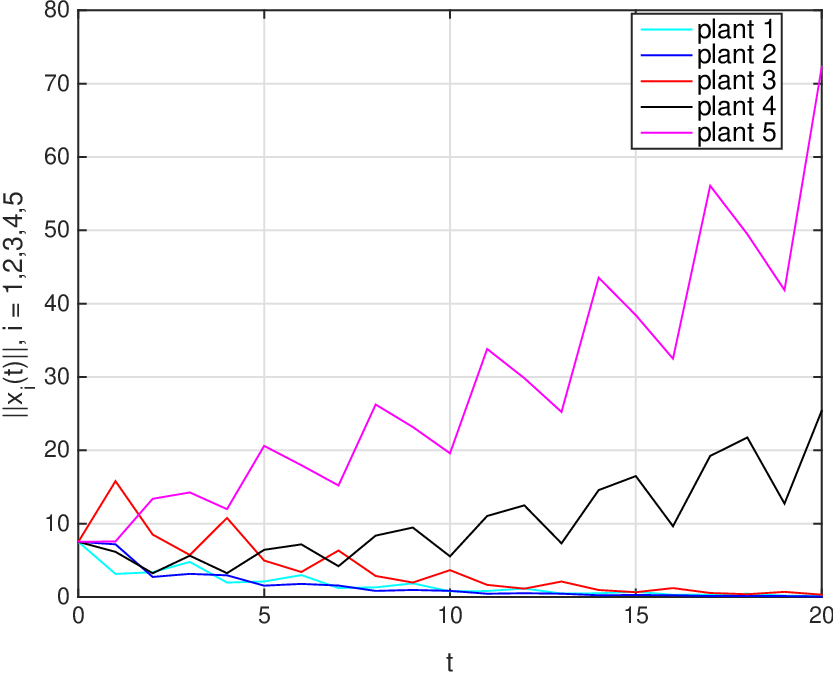
We note that designing a stabilizing scheduling policy in the above setting is not a trivial problem. Indeed, consider a round-robin scheduling policy plants 11 and 22 followed by plants 2 and 3 followed by plants 4 and 5 accessing the channel, each combination being active for 11 unit of time. In Figure 3 we demonstrate that the plants 44 and 55 are unstable under this scheduling policy, and consequently, a careful design of γ\gamma is essential.

5.1.3. The underlying weighted directed graph

We construct the underlying directed graph 𝒢⁡(𝒱,ℰ)\mathcal{G}(\mathcal{V},\mathcal{E}) of the NCS under consideration. For the given setting we have (NM)=10{N\choose M}=10. 𝒢\mathcal{G} consists of:

  • ∘\circ

    𝒱={v¯1,v¯2,…,v¯10}\mathcal{V}=\{\overline{v}_{1},\overline{v}_{2},\ldots,\overline{v}_{10}\} with
    L⁡(v¯1)={1s,2s,3u,4u,5u}L(\overline{v}_{1})=\{1_{s},2_{s},3_{u},4_{u},5_{u}\}, L⁡(v¯2)={1s,2u,3s,4u,5u}L(\overline{v}_{2})=\{1_{s},2_{u},3_{s},4_{u},5_{u}\}, L⁡(v¯3)={1s,2u,3u,4s,5u}L(\overline{v}_{3})=\{1_{s},2_{u},3_{u},4_{s},5_{u}\}, L⁡(v¯4)={1s,2u,3u,4u,5s}L(\overline{v}_{4})=\{1_{s},2_{u},3_{u},4_{u},5_{s}\},
    L⁡(v¯5)={1u,2s,3s,4u,5u}L(\overline{v}_{5})=\{1_{u},2_{s},3_{s},4_{u},5_{u}\}, L⁡(v¯6)={1u,2s,3u,4s,5u}L(\overline{v}_{6})=\{1_{u},2_{s},3_{u},4_{s},5_{u}\}, L⁡(v¯7)={1u,2s,3u,4u,5s}L(\overline{v}_{7})=\{1_{u},2_{s},3_{u},4_{u},5_{s}\}, L⁡(v¯8)={1u,2u,3s,4s,5u}L(\overline{v}_{8})=\{1_{u},2_{u},3_{s},4_{s},5_{u}\},
    L⁡(v¯9)={1u,2u,3s,4u,5s}L(\overline{v}_{9})=\{1_{u},2_{u},3_{s},4_{u},5_{s}\}, L⁡(v¯10)={1u,2u,3u,4s,5s}L(\overline{v}_{10})=\{1_{u},2_{u},3_{u},4_{s},5_{s}\}, and

  • ∘\circ

    ℰ={(v¯p,v¯q),p,q=1,2,…,10,p≠q}\mathcal{E}=\{(\overline{v}_{p},\overline{v}_{q}),\>\>p,q=1,2,\ldots,10,\>\>p\neq q\}.

5.1.4. A TT-contractive cycle

Fix a candidate contractive cycle W=v0,(v0,v1),v1,(v1,v2),v2,(v2,v0),v0W=v_{0},(v_{0},v_{1}),v_{1},(v_{1},v_{2}),v_{2},(v_{2},v_{0}),v_{0} on 𝒢\mathcal{G}, where v0=v¯5v_{0}=\overline{v}_{5}, v1=v¯4v_{1}=\overline{v}_{4}, v2=v¯10v_{2}=\overline{v}_{10}. We apply Algorithm 2 with hs=0.0001h_{s}=0.0001 and hu=0.1h_{u}=0.1, and obtain that WW is TT-contractive with TT-factors: Tv0=4T_{v_{0}}=4, Tv1=3T_{v_{1}}=3, Tv2=5T_{v_{2}}=5. Indeed, Ξ1​(W)=−2.7629\Xi_{1}(W)=-2.7629, Ξ2​(W)=−8.0877\Xi_{2}(W)=-8.0877, Ξ3​(W)=−7.9572\Xi_{3}(W)=-7.9572, Ξ4​(W)=−0.2626\Xi_{4}(W)=-0.2626, Ξ5​(W)=−5.8414\Xi_{5}(W)=-5.8414. The corresponding values of the scalars λp\lambda_{p}, p∈{is,iu}p\in\{i_{s},i_{u}\} and μp​q\mu_{pq}, p,q∈{is,iu}p,q\in\{i_{s},i_{u}\}, i=1,2,…,Ni=1,2,\ldots,N are given in Table 2.

ii λis\lambda_{i_{s}} λiu\lambda_{i_{u}} μis​iu\mu_{i_{s}i_{u}} μiu​is\mu_{i_{u}i_{s}}
11 0.13600.1360 1.23461.2346 2.84522.8452 1.32321.3232
22 0.07200.0720 1.23461.2346 1.56811.5681 1.35091.3509
33 0.07150.0715 1.23461.2346 1.90251.9025 1.30461.3046
44 0.17570.1757 2.77782.7778 3.08543.0854 1.16651.1665
55 0.24300.2430 2.77782.7778 3.46643.4664 1.15761.1576
Table 2. Description of scalars admitting a solution to feasibility problem (24)

5.1.5. The scheduling policy

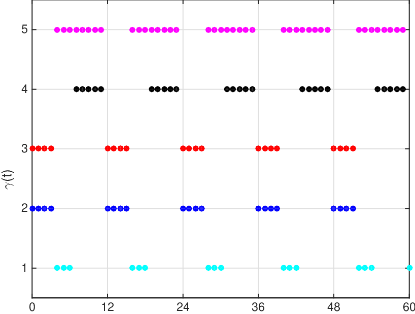
A scheduling policy γ\gamma is obtained from Algorithm 1. γ\gamma is constructed by employing WW, and it is periodic with period Tv0+Tv1+Tv2=12T_{v_{0}}+T_{v_{1}}+T_{v_{2}}=12 units of time. In Figure 4 we illustrate γ\gamma until time t=60t=60.

Refer to caption
Figure 4. Scheduling policy γ\gamma obtained from Algorithm 1

5.1.6. GAS of NCS

We choose 100 different initial conditions from the interval [−10,10]2[-10,10]^{2} uniformly at random, and plot (‖xi​(t)‖)t∈ℕ0(\left\lVert x_{i}(t)\right\rVert)_{t\in\mathbb{N}_{0}} under the scheduling policy γ\gamma, i=1,2,3,4,5i=1,2,3,4,5. Figure 5 contains plots for ‖xi​(t)‖\left\lVert x_{i}(t)\right\rVert, i=1,2,3,4,5i=1,2,3,4,5 until time t=60t=60. It is observed that the individual plants of the NCS under consideration are GAS under our scheduling policy.

Refer to caption
Refer to caption
Refer to caption

Refer to caption Refer to caption

Figure 5. Plot for ‖xi​(t)‖\left\lVert x_{i}(t)\right\rVert versus tt for each plant i=1,2,3,4,5i=1,2,3,4,5

5.1.7. Comparison

We choose three distinct TT-contractive cycles Wj=v0(j),(v0(j),v1(j)),v1(j),(v1(j),v2(j)),v2(j),(v2(j),v0(j)),v0(j)W_{j}=v_{0}^{(j)},(v_{0}^{(j)},v_{1}^{(j)}),v_{1}^{(j)},(v_{1}^{(j)},v_{2}^{(j)}),v_{2}^{(j)},(v_{2}^{(j)},v_{0}^{(j)}),v_{0}^{(j)} on 𝒢\mathcal{G}. The description of the cycles and the corresponding values of Ξi​(Wj)\Xi_{i}(W_{j}), j=1,2,3j=1,2,3, i=1,2,3,4,5i=1,2,3,4,5 are given in Table 3.

jj v0v_{0} v1v_{1} v2v_{2} Tv0T_{v_{0}} Tv1T_{v_{1}} Tv2T_{v_{2}} Ξ1​(Wj)\Xi_{1}(W_{j}) Ξ2​(Wj)\Xi_{2}(W_{j}) Ξ3​(Wj)\Xi_{3}(W_{j}) Ξ4​(Wj)\Xi_{4}(W_{j}) Ξ5​(Wj)\Xi_{5}(W_{j})
11 v¯5\overline{v}_{5} v¯3\overline{v}_{3} v¯9\overline{v}_{9} 22 77 88 −10.5325-10.5325 −1.3503-1.3503 −23.9963-23.9963 −0.67556-0.67556 −0.73315-0.73315
22 v¯2\overline{v}_{2} v¯6\overline{v}_{6} v¯7\overline{v}_{7} 33 88 99 −1.0769-1.0769 −43.3456-43.3456 −3.4224-3.4224 −0.37122-0.37122 −0.10453-0.10453
33 v¯8\overline{v}_{8} v¯9\overline{v}_{9} v¯1\overline{v}_{1} 88 99 33 −1.0769-1.0769 −3.5599-3.5599 −43.3057-43.3057 −0.37122-0.37122 −0.10453-0.10453
Table 3. Description of different TT-contractive cycles on 𝒢\mathcal{G}

We now illustrate that with smaller values of Ξi​(Wj)\Xi_{i}(W_{j}), the rate of convergence of ‖xi​(t)‖\left\lVert x_{i}(t)\right\rVert to 00 becomes faster. For this purpose, we pick 10 different initial conditions xi​(0)x_{i}(0) from the interval [−1,1]2[-1,1]^{2} uniformly at random and simulate (‖xi​(t)‖)t∈ℕ0(\left\lVert x_{i}(t)\right\rVert)_{t\in\mathbb{N}_{0}} for the cycles WjW_{j}. Figure 6 contains plots for averagexi​(0)⁡(‖xi​(t)‖)t∈ℕ0\displaystyle{\average_{x_{i}(0)}}({\left\lVert x_{i}(t)\right\rVert})_{t\in\mathbb{N}_{0}} for the plant i=3i=3 corresponding to the cycles WjW_{j}.

Refer to caption
Figure 6. Plot for averagex3​(0)⁡‖x3​(t)‖\average_{x_{3}(0)}\left\lVert x_{3}(t)\right\rVert versus tt corresponding to cycles WjW_{j}.

5.2. Experiment 2

We now test the performance of our techniques in large scale settings. This involves a three-step procedure:

  • ∘\circ

    First, we generate NN non-Schur matrices Ai∈ℝ2×2A_{i}\in\mathbb{R}^{2\times 2} and vectors Bi∈ℝ2×1B_{i}\in\mathbb{R}^{2\times 1} with entries from the interval [−2,2][-2,2] and the set {0,1}\{0,1\}, respectively, chosen uniformly at random, and ensuring that each pair (Ai,Bi)(A_{i},B_{i}), i=1,2,…,Ni=1,2,\ldots,N, is controllable. The associated linear quadratic regulators KiK_{i} are computed with Qi=Q=5​I2×2Q_{i}=Q=5I_{2\times 2} and Ri=R=1R_{i}=R=1.

  • ∘\circ

    Second, the underlying directed graph 𝒢\mathcal{G} of the NCS is considered, and a candidate contractive cycle W=v0,(v0,v1),v1,…W=v_{0},(v_{0},v_{1}),v_{1},\ldots,
    vn−1,(vn−1,v0),v0v_{n-1},(v_{n-1},v_{0}),v_{0} on 𝒢\mathcal{G} is chosen in the following manner:

    • ⋄\diamond

      Fix M=10M=10. We pick 1010 distinct numbers from the set {1,2,…,N}\{1,2,\ldots,N\} uniformly at random, and repeat this process until each element of {1,2,…,N}\{1,2,\ldots,N\} is picked at least once.

    • ⋄\diamond

      For each set of 1010 distinct numbers picked above, we choose a vertex vv on 𝒢\mathcal{G} that satisfies ℓv​(i)=is\ell_{v}(i)=i_{s} for these numbers. WW is constructed by concatenating these vertices neglecting repetitions.

  • ∘\circ

    Third, Algorithm 2 is employed with the chosen AiA_{i}, BiB_{i}, KiK_{i} and WW to design the scalars λis\lambda_{i_{s}}, λiu\lambda_{i_{u}}, μis​iu\mu_{i_{s}i_{u}}, μiu​is\mu_{i_{u}i_{s}}, i=1,2,…,Ni=1,2,\ldots,N for TT-contractivity of WW. The step-sizes are chosen as hs=hu=0.001h_{s}=h_{u}=0.001.

We repeat the above procedure for large values of NN and study the total computation times. The procedure is implemented on a MATLAB platform.66 6 Version: R2015a, System specifications: Intel Core i7 processor, 8GB RAM, 64-bit OS. In Table 4 we list sizes of 𝒢\mathcal{G} and lengths of candidate contractive cycles W=v0,(v0,v1),v1,…,vn−1W=v_{0},(v_{0},v_{1}),v_{1},\ldots,v_{n-1},
(vn−1,v0),v0(v_{n-1},v_{0}),v_{0} for various values of NN, and the computation times. In case of N=700N=700, the first choice of candidate contractive cycle WW did not turn out to be TT-contractive from Algorithm 2. We then repeated the process of generating a candidate contractive cycle, and obtained a solution from Algorithm 2 for the new choice of WW.

NN |𝒱|\left\lvert{\mathcal{V}}\right\rvert nn Computation time (sec)
100100 1.73×10131.73\times 10^{13} 6161 4681.77
200200 2.24×10162.24\times 10^{16} 104104 7966.65
500500 2.45×10202.45\times 10^{20} 345345 35268.59
700700 7.3×10217.3\times 10^{21} 532532 76746.32
10001000 2.63×10232.63\times 10^{23} 822822 70453.28
Table 4. Graph and cycle data

6. Concluding remarks

In this paper we presented a stabilizing scheduling policy for NCSs under medium access constraints. A switched system representation is associated to the individual plants, and a weighted directed graph is associated to the NCS. Our scheduling policy is designed by employing a TT-contractive cycle on the underlying weighted directed graph of the NCS. We also address algorithmic construction of TT-contractive cycles. Since our algorithm for designing TT-contractive cycles does not conclude about their non-existence, an important question is regarding the design of such cycles when our algorithm does not yield a solution for all choices of candidate contractive cycle on a weighted directed graph. Also, a natural extension of our work is to accommodate network induced uncertainties such as access delays, packet dropouts, etc. in the feedback control loop. These aspects are currently under investigation and will be reported elsewhere.

7. Proofs of results

Proof of Theorem 1.

Consider the NCS described in §2 and its underlying directed graph 𝒢⁡(𝒱,ℰ)\mathcal{G}(\mathcal{V},\mathcal{E}). Let W=v0,(v0,v1),v1,…W=v_{0},(v_{0},v_{1}),v_{1},\ldots,
vn−1,(vn−1,v0),v0v_{n-1},(v_{n-1},v_{0}),v_{0} be a TT-contractive cycle on 𝒢\mathcal{G}. Consider a scheduling policy γ\gamma obtained from Algorithm 1 constructed by employing WW. We will show that each plant in (1) is GAS under γ\gamma.

Fix an arbitrary plant i∈{1,2,…,N}i\in\{1,2,\ldots,N\}. In view of the switched systems representation of plant ii in (3), it suffices to show that the switching logic σi\sigma_{i} corresponding to γ\gamma, ensures GAS of plant ii.

Fix a time t∈ℕt\in\mathbb{N}. Recall that 0=:τ0<τ1<⋯0=:\tau_{0}<\tau_{1}<\cdots are the points in time at which γ\gamma changes values. Let NtγN^{\gamma}_{t} be the total number of times γ\gamma has changed its values on ]0:t]]0:t]. In view of (5), we have

(18) Vσi​(t)​(xi​(t))≤λσi​(τNtγ)t−τNtγ​Vσi​(τNtγ)​(xi​(τNtγ)).\displaystyle V_{\sigma_{i}(t)}(x_{i}(t))\leq\lambda_{\sigma_{i}(\tau_{N^{\gamma}_{t}})}^{t-\tau_{N^{\gamma}_{t}}}V_{\sigma_{i}(\tau_{N^{\gamma}_{t}})}(x_{i}(\tau_{N^{\gamma}_{t}})).

A straightforward iteration of (18) using (5) and (6) gives

(19) Vσi​(t)(xi(t))≤(∏j=0τNtγ+1:=tNtγλσi​(τj)τj+1−τj⋅∏j=0Ntγ−1μσi​(τj)​σi​(τj+1))Vσi​(0)(xi(0)).\displaystyle V_{\sigma_{i}(t)}(x_{i}(t))\leq\Biggl(\prod_{\begin{subarray}{c}{j=0}\\ {\tau_{N^{\gamma}_{t}+1}:=t}\end{subarray}}^{N^{\gamma}_{t}}\lambda_{\sigma_{i}(\tau_{j})}^{\tau_{j+1}-\tau_{j}}\cdot\prod_{j=0}^{N^{\gamma}_{t}-1}\mu_{\sigma_{i}(\tau_{j})\sigma_{i}(\tau_{j+1})}\Biggr)V_{\sigma_{i}(0)}(x_{i}(0)).

The first term on the right-hand side of the above inequality can be rewritten as

exp(ln(∏j=0τNtγ+1:=tNtγλσi​(τj)τj+1−τj)+ln(∏j=0Ntγ−1μσi​(τj)​σi​(τj+1))).\displaystyle\exp\Biggl(\ln\Biggl(\prod_{\begin{subarray}{c}{j=0}\\ {\tau_{N^{\gamma}_{t}+1}:=t}\end{subarray}}^{N^{\gamma}_{t}}\lambda_{\sigma_{i}(\tau_{j})}^{\tau_{j+1}-\tau_{j}}\Biggr)+\ln\Biggl(\prod_{j=0}^{N^{\gamma}_{t}-1}\mu_{\sigma_{i}(\tau_{j})\sigma_{i}(\tau_{j+1})}\Biggr)\Biggr).

Now,

(20) ln(∏j=0τNtγ+1:=tNtγλσi​(τj)τj+1−τj)=∑j=0τNtγ+1:=tNtγ(τj+1−τj)lnλσi​(τj)=∑j=0τNtγ+1:=tNtγ(∑p∈{is,iu}1(σi(τj)=p)(τj+1−τj)lnλp).\displaystyle\ln\Biggl(\prod_{\begin{subarray}{c}{j=0}\\ {\tau_{N^{\gamma}_{t}+1}:=t}\end{subarray}}^{N^{\gamma}_{t}}\lambda_{\sigma_{i}(\tau_{j})}^{\tau_{j+1}-\tau_{j}}\Biggr)=\sum_{\begin{subarray}{c}{j=0}\\ {\tau_{N^{\gamma}_{t}+1}:=t}\end{subarray}}^{N^{\gamma}_{t}}(\tau_{j+1}-\tau_{j})\ln\lambda_{\sigma_{i}(\tau_{j})}=\sum_{\begin{subarray}{c}{j=0}\\ \tau_{N^{\gamma}_{t}+1}:=t\end{subarray}}^{N^{\gamma}_{t}}\biggl(\sum_{p\in\{i_{s},i_{u}\}}\mathrm{1}(\sigma_{i}(\tau_{j})=p)(\tau_{j+1}-\tau_{j})\ln\lambda_{p}\biggr).

Let Ds​(s,t)D_{s}(s,t) and Du​(s,t)D_{u}(s,t) denote the total durations number of time-steps of activation of the stable and unstable modes of ii on ]s:t]]s:t], respectively. Recall that 0<λis<10<\lambda_{i_{s}}<1 and λiu≥1\lambda_{i_{u}}\geq 1. Consequently, ln⁡λis<0\ln\lambda_{i_{s}}<0 and ln⁡λiu≥0\ln\lambda_{i_{u}}\geq 0. Thus, the right-hand side of (20) is equal to

(21) −|ln⁡λis|​Ds​(0,t)+|ln⁡λiu|​Du​(0,t).\displaystyle-\left\lvert{\ln\lambda_{i_{s}}}\right\rvert D_{s}(0,t)+\left\lvert{\ln\lambda_{i_{u}}}\right\rvert D_{u}(0,t).

Let Np​q​(s,t)N_{pq}(s,t) denote the total number of transitions from subsystem (mode) pp to subsystem (mode) qq, p,q∈{is,iu}p,q\in\{i_{s},i_{u}\} on ]s:t]]s:t]. We have

ln⁡(∏j=0Ntγ−1μσi​(τj)​σi​(τj+1))=∑j=0Ntγ−1ln⁡μσi​(τj)​σi​(τj+1)\displaystyle\ln\Biggl(\prod_{j=0}^{N^{\gamma}_{t}-1}\mu_{\sigma_{i}(\tau_{j})\sigma_{i}(\tau_{j+1})}\Biggr)=\sum_{j=0}^{N^{\gamma}_{t}-1}\ln\mu_{\sigma_{i}(\tau_{j})\sigma_{i}(\tau_{j+1})} =∑p∈{is,iu}∑j=0Ntγ−1∑p→q:q∈{is,iu},σi​(τj)=p,σi​(τj+1)=qlnμp​q\displaystyle=\sum_{p\in\{i_{s},i_{u}\}}\sum_{j=0}^{N^{\gamma}_{t}-1}\sum_{\begin{subarray}{c}{p\to q:}\\ {q\in\{i_{s},i_{u}\},}\\ {\sigma_{i}(\tau_{j})=p,}\\ {\sigma_{i}(\tau_{j+1})=q}\end{subarray}}\ln\mu_{pq}
(22) =ln⁡μis​iu​Nis​iu​(0,t)+ln⁡μiu​is​Niu​is​(0,t),\displaystyle=\ln\mu_{i_{s}i_{u}}N_{i_{s}i_{u}}(0,t)+\ln\mu_{i_{u}i_{s}}N_{i_{u}i_{s}}(0,t),

since μis​is=μiu​iu=1\mu_{i_{s}i_{s}}=\mu_{i_{u}i_{u}}=1. Substituting (21) and (7) in (19), we obtain

(23) Vσi​(t)​(xi​(t))≤ψi​(t)​Vσi​(0)​(xi​(0)),\displaystyle V_{\sigma_{i}(t)}(x_{i}(t))\leq\psi_{i}(t)V_{\sigma_{i}(0)}(x_{i}(0)),

where

(24) ℕ∋t↦ψi​(t)\displaystyle\mathbb{N}\ni t\mapsto\psi_{i}(t) :=exp⁡(−|ln⁡λis|​Ds​(0,t)+|ln⁡λiu|​Du​(0,t)+ln⁡μis​iu​Nis​iu​(0,t)+ln⁡μiu​is​Niu​is​(0,t)).\displaystyle:=\exp\Biggl(-\left\lvert{\ln\lambda_{i_{s}}}\right\rvert D_{s}(0,t)+\left\lvert{\ln\lambda_{i_{u}}}\right\rvert D_{u}(0,t)+\ln\mu_{i_{s}i_{u}}N_{i_{s}i_{u}}(0,t)+\ln\mu_{i_{u}i_{s}}N_{i_{u}i_{s}}(0,t)\Biggr).

From the definition of VpV_{p}, p∈{is,iu}p\in\{i_{s},i_{u}\} in (4) and properties of positive definite matrices [2, Lemma 8.4.3], it follows that

(25) ‖xi​(t)‖≤c​ψi​(t)​‖xi​(0)‖​for all​t∈ℕ0,\displaystyle\left\lVert x_{i}(t)\right\rVert\leq c\psi_{i}(t)\left\lVert x_{i}(0)\right\rVert\>\>\text{for all}\>\>t\in\mathbb{N}_{0},

where c=maxp∈{is,iu}⁡λmax​(Pp)minp∈{is,iu}⁡λmin​(Pp)\displaystyle{c=\sqrt{\frac{\displaystyle{\max_{p\in\{i_{s},i_{u}\}}\lambda_{\max}(P_{p})}}{\displaystyle{\min_{p\in\{i_{s},i_{u}\}}\lambda_{\min}(P_{p})}}}}, where for a matrix A∈ℝd×dA\in\mathbb{R}^{d\times d}, λmin​(A)\lambda_{\min}(A) denotes the minimum eigenvalue of AA. By Definition 1, to establish GAS of (3), we need to show that c⁡‖xi​(0)‖​ψi​(t)c\left\lVert x_{i}(0)\right\rVert\psi_{i}(t) can be bounded above by a class 𝒦​ℒ\mathcal{KL} function. Towards this end, we already see that c​‖xi​(0)‖c\left\lVert x_{i}(0)\right\rVert is a class 𝒦∞\mathcal{K}_{\infty} function. Therefore, it remains to show that ψi​(t)\psi_{i}(t) is bounded above by a function in class ℒ\mathcal{L}.

Recall that γ\gamma is constructed by employing a TT-contractive cycle W=v0,(v0,v1),v1,…,vn−1,(vn−1,v0),v0W=v_{0},(v_{0},v_{1}),v_{1},\ldots,v_{n-1},(v_{n-1},v_{0}),v_{0} on 𝒢\mathcal{G}, and TvjT_{v_{j}}, j=0,1,…,n−1j=0,1,\ldots,n-1 are the TT-factors associated to vertices vjv_{j}, j=0,1,…,n−1j=0,1,\ldots,n-1. Let TW:=∑j=0n−1Tvj\displaystyle{T_{W}:=\sum_{j=0}^{n-1}T_{v_{j}}}, t≥m​TWt\geq mT_{W}, m∈ℕ0m\in\mathbb{N}_{0}, and Ξi​(W)=−εi\Xi_{i}(W)=-\varepsilon_{i}, εi>0\varepsilon_{i}>0, where Ξi​(W)\Xi_{i}(W) is as defined in (9). By construction of γ\gamma, we have

ψi​(t)\displaystyle\psi_{i}(t) =exp⁡(−|ln⁡λis|​Ds​(0,t)+|ln⁡λiu|​Du​(0,t)+ln⁡μis​iu​Nis​iu​(0,t)+ln⁡μiu​is​Niu​is​(0,t))\displaystyle=\exp\Biggl(-\left\lvert{\ln\lambda_{i_{s}}}\right\rvert D_{s}(0,t)+\left\lvert{\ln\lambda_{i_{u}}}\right\rvert D_{u}(0,t)+\ln\mu_{i_{s}i_{u}}N_{i_{s}i_{u}}(0,t)+\ln\mu_{i_{u}i_{s}}N_{i_{u}i_{s}}(0,t)\Biggr)
=−|ln⁡λis|​Ds​(0,m​TW)−|ln⁡λis|​Ds​(m​TW,t)+|ln⁡λiu|​Du​(0,m​TW)+|ln⁡λiu|​Du​(m​TW,t)\displaystyle=-\left\lvert{\ln\lambda_{i_{s}}}\right\rvert D_{s}(0,mT_{W})-\left\lvert{\ln\lambda_{i_{s}}}\right\rvert D_{s}(mT_{W},t)+\left\lvert{\ln\lambda_{i_{u}}}\right\rvert D_{u}(0,mT_{W})+\left\lvert{\ln\lambda_{i_{u}}}\right\rvert D_{u}(mT_{W},t)
(26) +ln⁡μis​iu​Nis​iu​(0,m​TW)+ln⁡μis​iu​Nis​iu​(m​TW,t)+ln⁡μiu​is​Niu​is​(0,m​TW)+ln⁡μiu​is​Niu​is​(m​TW,t).\displaystyle\>\>\>\>\>+\ln\mu_{i_{s}i_{u}}N_{i_{s}i_{u}}(0,mT_{W})+\ln\mu_{i_{s}i_{u}}N_{i_{s}i_{u}}(mT_{W},t)+\ln\mu_{i_{u}i_{s}}N_{i_{u}i_{s}}(0,mT_{W})+\ln\mu_{i_{u}i_{s}}N_{i_{u}i_{s}}(mT_{W},t).

Notice that

−|ln⁡λis|​Ds​(0,m​TW)+|ln⁡λiu|​Du​(0,m​TW)+ln⁡μis​iu​Nis​iu​(0,m​TW)+ln⁡μiu​is​Niu​is​(0,m​TW)\displaystyle-\left\lvert{\ln\lambda_{i_{s}}}\right\rvert D_{s}(0,mT_{W})+\left\lvert{\ln\lambda_{i_{u}}}\right\rvert D_{u}(0,mT_{W})+\ln\mu_{i_{s}i_{u}}N_{i_{s}i_{u}}(0,mT_{W})+\ln\mu_{i_{u}i_{s}}N_{i_{u}i_{s}}(0,mT_{W})
=−|lnλis|m∑j:ℓvj​(i)=isj=0,1,…,n−1Tvj+|lnλiu|m∑j:ℓvj​(i)=iuj=0,1,…,n−1Tvj+lnμis​ium#(is→iu)W+lnμiu​ism#(iu→is)W,\displaystyle=-\left\lvert{\ln\lambda_{i_{s}}}\right\rvert m\sum_{\begin{subarray}{c}{j:\ell_{v_{j}}(i)=i_{s}}\\ {j=0,1,\ldots,n-1}\end{subarray}}T_{v_{j}}+\left\lvert{\ln\lambda_{i_{u}}}\right\rvert m\sum_{\begin{subarray}{c}{j:\ell_{v_{j}}(i)=i_{u}}\\ {j=0,1,\ldots,n-1}\end{subarray}}T_{v_{j}}+\ln\mu_{i_{s}i_{u}}m\#(i_{s}\to i_{u})_{W}+\ln\mu_{i_{u}i_{s}}m\#(i_{u}\to i_{s})_{W},

where #​(p→q)W\#(p\to q)_{W} denotes the number of times a transition from a vertex vjv_{j} to a vertex vj+1v_{j+1} has occurred in WW such that ℓvj​(i)=p\ell_{v_{j}}(i)=p and ℓvj+1​(i)=q\ell_{v_{j+1}}(i)=q, p,q∈{is,iu}p,q\in\{i_{s},i_{u}\}, p≠qp\neq q. The right-hand side of the above equality can be rewritten as

(27) m(−|lnλis|∑j:ℓvj​(i)=isj=0,1,…,n−1Tvj\displaystyle m\Biggl(-\left\lvert{\ln\lambda_{i_{s}}}\right\rvert\sum_{\begin{subarray}{c}{j:\ell_{v_{j}}(i)=i_{s}}\\ {j=0,1,\ldots,n-1}\end{subarray}}T_{v_{j}} +|lnλiu|∑j:ℓvj​(i)=iuj=0,1,…,n−1Tvj+lnμis​iu#(is→iu)W+lnμiu​is#(iu→is)W).\displaystyle+\left\lvert{\ln\lambda_{i_{u}}}\right\rvert\sum_{\begin{subarray}{c}{j:\ell_{v_{j}}(i)=i_{u}}\\ {j=0,1,\ldots,n-1}\end{subarray}}T_{v_{j}}+\ln\mu_{i_{s}i_{u}}\#(i_{s}\to i_{u})_{W}+\ln\mu_{i_{u}i_{s}}\#(i_{u}\to i_{s})_{W}\Biggr).

From the definition of weights associated to vertices and edges of 𝒢\mathcal{G}, we have that the above expression is equal to −m​εi-m\varepsilon_{i}. Also,

−|ln⁡λis|​Ds​(m​TW,t)+|ln⁡λiu|​Du​(m​TW,t)+ln⁡μis​iu​Nis​iu​(m​TW,t)+ln⁡μiu​is​Niu​is​(m​TW,t)\displaystyle-\left\lvert{\ln\lambda_{i_{s}}}\right\rvert D_{s}(mT_{W},t)+\left\lvert{\ln\lambda_{i_{u}}}\right\rvert D_{u}(mT_{W},t)+\ln\mu_{i_{s}i_{u}}N_{i_{s}i_{u}}(mT_{W},t)+\ln\mu_{i_{u}i_{s}}N_{i_{u}i_{s}}(mT_{W},t)
(28) ≤|ln⁡λiu|​(t−m​TW)+m​n​(ln⁡μis​iu+ln⁡μiu​is):=a​(say).\displaystyle\leq\left\lvert{\ln\lambda_{i_{u}}}\right\rvert(t-mT_{W})+mn(\ln\mu_{i_{s}i_{u}}+\ln\mu_{i_{u}i_{s}}):=a\>\text{(say)}.

From (27) and (7), we obtain that the right-hand side of (7) is bounded above by exp⁡(−m​εi+a)\exp\bigl(-m\varepsilon_{i}+a\bigr).

Let φi:[0,t]→ℝ\varphi_{i}:[0,\>t]\to\mathbb{R} be a function connecting (0,exp⁡(a)+TW)(0,\exp(a)+T_{W}), (r​TW,exp⁡(−(r−1)​εi+a))(rT_{W},\exp(-(r-1)\varepsilon_{i}+a)), (t,exp⁡(−m​εi+a))(t,\exp(-m\varepsilon_{i}+a)), r=1,2,…,mr=1,2,\ldots,m, with straight line segments. By construction, φi\varphi_{i} is an upper envelope of T↦ψi​(T)T\mapsto\psi_{i}(T) on [0,t][0{,}t], is continuous, decreasing, and tends to 00 as t→+∞t\to+\infty. Hence, φi∈ℒ\varphi_{i}\in\mathcal{L}.

Recall that i∈{1,2,…,N}i\in\{1,2,\ldots,N\} was selected arbitrarily. It follows that our assertion holds for all plants ii in (1). ∎

Remark 15.

Our scheduling policy γ\gamma is constructed by employing TT-contractive cycles on 𝒢\mathcal{G}. The definition of the functions ψt\psi_{t}, i=1,2,…,Ni=1,2,\ldots,N clarifies the association of natural logarithm with the scalars λp\lambda_{p}, p∈{is,iu}p\in\{i_{s},i_{u}\} and μp​q\mu_{pq}, p,q∈{is,iu}p,q\in\{i_{s},i_{u}\} in the vertex and edge weights of 𝒢\mathcal{G}, respectively, i=1,2,…,Ni=1,2,\ldots,N. The use of absolute values with ln⁡λp\ln\lambda_{p}, p∈{is,iu}p\in\{i_{s},i_{u}\}, i=1,2,…,Ni=1,2,\ldots,N allows for an easy distinction between the positive and negative terms in ψi\psi_{i}, i=1,2,…,Ni=1,2,\ldots,N. Alternatively, one may exclude the absolute values and keep track of which terms are negative in the subsequent analysis.

Proof of Proposition 1.

Let M=1M=1. Fix a cycle W=v0,(v0,v1),v1,…,vN−1,(vN−1,v0),v0W=v_{0},(v_{0},v_{1}),v_{1},\ldots,v_{N-1},(v_{N-1},v_{0}),v_{0} on 𝒢\mathcal{G} that satisfies vks∩vℓs=∅v_{k}^{s}\cap v_{\ell}^{s}=\emptyset for all k,ℓ=0,1,…,N−1k,\ell=0,1,\ldots,N-1, l≠ℓl\neq\ell. Clearly, WW is a candidate contractive cycle on 𝒢\mathcal{G}.

Without loss of generality, let us assume that ℓvi−1​(i)=is\ell_{v_{i-1}}(i)=i_{s}, i=1,2,…,Ni=1,2,\ldots,N. Suppose that Tvj=T~T_{v_{j}}=\tilde{T}, j=0,1,…,N−1j=0,1,\ldots,N-1. By construction of WW, the left-hand side of (11) is

−|ln⁡λis|​Tvi−1+|ln⁡λiu|​(∑j=0j≠i−1N−1Tvj)+ln⁡μis​iu+ln⁡μiu​is\displaystyle-\left\lvert{\ln\lambda_{i_{s}}}\right\rvert T_{v_{i-1}}+\left\lvert{\ln\lambda_{i_{u}}}\right\rvert\Bigl(\sum_{\begin{subarray}{c}j=0\\ j\neq i-1\end{subarray}}^{N-1}T_{v_{j}}\Bigr)+\ln\mu_{i_{s}i_{u}}+\ln\mu_{i_{u}i_{s}}
=\displaystyle= (−|ln⁡λis|+(N−1)​|ln⁡λiu|)​T~+ln⁡μis​iu+ln⁡μiu​is,i=1,2,…,N.\displaystyle\Bigl(-\left\lvert{\ln\lambda_{i_{s}}}\right\rvert+(N-1)\left\lvert{\ln\lambda_{i_{u}}}\right\rvert\Bigr)\tilde{T}+\ln\mu_{i_{s}i_{u}}+\ln\mu_{i_{u}i_{s}},\>i=1,2,\ldots,N.

Since (16) holds, it is possible to choose an integer T~>0\tilde{T}>0 such that the above expression is strictly less than 00. ∎

Proof of Proposition 2.

Let M≥N/2\displaystyle{M\geq{N}/{2}}. Fix a cycle W=v0,(v0,v1),v1,(v1,v0),v0W=v_{0},(v_{0},v_{1}),v_{1},(v_{1},v_{0}),v_{0} on 𝒢\mathcal{G} that satisfies v1s⊃{1,2,…,N}∖V0sv_{1}^{s}\supset\{1,2,\ldots,N\}\setminus V_{0}^{s}. Let j1,j2,…,jMj_{1},j_{2},\ldots,j_{M} and k1,k2,…,kN−M∈{1,2,…,N}k_{1},k_{2},\ldots,k_{N-M}\in\{1,2,\ldots,N\} be the elements for which ℓv0​(jp)=jps\ell_{v_{0}}(j_{p})=j_{p_{s}}, p=1,2,…,Mp=1,2,\ldots,M and ℓv1​(kq)=kqs\ell_{v_{1}}(k_{q})=k_{q_{s}}, q=1,2,…,N−Mq=1,2,\ldots,N-M, respectively. We have |{j1,j2,…,jM}|≥|k1,k2,…,kN−M|\left\lvert{\{j_{1},j_{2},\ldots,j_{M}\}}\right\rvert\geq\left\lvert{k_{1},k_{2},\ldots,k_{N-M}}\right\rvert. It is immediate that WW is a candidate contractive cycle.

Suppose that Tv0=Tv1=T~T_{v_{0}}=T_{v_{1}}=\tilde{T}. By construction of WW, we have N¯is​iu\overline{N}_{i_{s}i_{u}}, N¯iu​is∈{0,1}\overline{N}_{i_{u}i_{s}}\in\{0,1\}, i=1,2,…,Ni=1,2,\ldots,N. The left-hand side of (11) is bounded above by

(−|ln⁡λis|+|ln⁡λiu|)​T~+ln⁡μis​iu+ln⁡μiu​is.\Bigl(-\left\lvert{\ln\lambda_{i_{s}}}\right\rvert+\left\lvert{\ln\lambda_{i_{u}}}\right\rvert\Bigr)\tilde{T}+\ln\mu_{i_{s}i_{u}}+\ln\mu_{i_{u}i_{s}}.

Since condition (17) holds, there exists T~>0\tilde{T}>0 such that the above expression is strictly less than 00. ∎

References

  • [1] S. Al-Areqi, D. Görges, and S. Liu, Event-based control and scheduling codesign: stochastic and robust approaches, IEEE Transactions on Automatic Control, 60 (2015), pp. 1291–1303.
  • [2] D. S. Bernstein, Matrix mathematics, Princeton University Press, Princeton, NJ, second ed., 2009. Theory, facts, and formulas.
  • [3] B. Bollobás, Modern graph theory, vol. 184 of Graduate Texts in Mathematics, Springer-Verlag, New York, 1998.
  • [4] M. S. Branicky, Multiple Lyapunov functions and other analysis tools for switched and hybrid systems, IEEE Trans. Automat. Control, 43 (1998), pp. 475–482. Hybrid control systems.
  • [5] S.-L. Dai, H. Lin, and S. S. Ge, Scheduling-and-control codesign for a collection of networked control systems with uncertain delays, IEEE Transactions on Control Systems Technology, 18 (2010), pp. 66–78.
  • [6] D. Han, J. Wu, Y. Mo, and L. Xie, On stochastic sensor network scheduling for multiple processes, IEEE Trans. Automat. Control, 62 (2017), pp. 6633–6640.
  • [7] A. Hassibi, S. Boyd, and J. How, A class of lyapunov functionals for analyzing hybrid dynamical systems. Proceedings of American Control Conference, 1999, pp. 2455–2460.
  • [8] Q. He, V. Angelakis, A. Ephremides, and D. Yuan, Polynomial complexity minimum-time scheduling in a class of wireless networks, IEEE Transactions on Control of Netw. Syst., 3 (2016), pp. 322–331.
  • [9] D. Hristu-Varsakelis, Feedback control systems as users of a shared network: Communication sequences that guarantee stability. Proceedings of the 40th IEEE Conference on Decision and Control, 2001, Orlando, Florida, USA, pp. 3631-3636.
  • [10] D. Hristu-Varsakelis, Short-period communication and the role of zero-order holding in networked control systems, IEEE Trans. Automat. Control, 53 (2008), pp. 1285–1290.
  • [11] D. Hristu-Varsakelis and L. Zhang, LQG control of networked control systems with access constraints and delays, Internat. J. Control, 81 (2008), pp. 1266–1280.
  • [12] D. Hristu-Versakelis, Feedback control with communication constraints. In D. Hristu-Varsakelis, W. S. Levine (Eds.), Handbook of networked and embedded systems, Boston/Basel/Berlin: Birkhäuser, 2005.
  • [13] H. Ishii and B. A. Francis, Stabilizing a linear system by switching control with dwell time, IEEE Trans. Automat. Control, 47 (2002), pp. 1962–1973.
  • [14] H. K. Khalil, Nonlinear Systems, Prentice-Hall, Englewood Cliffs, NJ, 2nd ed., 1996.
  • [15] A. Kundu, Stabilizing switched nonlinear systems under restricted switching. Proceedings of the 21st ACM International Conference on Hybrid Systems: Computation & Control, 2018, Porto, Portugal, pp. 101-110.
  • [16] A. Kundu and D. Chatterjee, Stabilizing discrete-time switched linear systems. Proceedings of the 17th ACM International Conference on Hybrid Systems: Computation & Control, 2014, Berlin, Germany, pp. 11-20.
  • [17]  , On stability of discrete-time switched systems, Nonlinear Analysis: Hybrid Systems (Special Issue: HSCC), 23 (2017), pp. 191–210.
  • [18] A. S. Leong, S. Dey, and D. E. Quevedo, Sensor scheduling in variance based event triggered estimation with packet drops, IEEE Trans. Automat. Control, 62 (2017), pp. 1880–1895.
  • [19] Y. Li, J. Wu, and T. Chen, Transmit power control and remote state estimation with sensor networks: A bayesian inference approach, Automatica, 97 (2018), pp. 292–300.
  • [20] D. Liberzon, Switching in systems and control, Systems & Control: Foundations & Applications, Birkhäuser Boston Inc., Boston, MA, 2003.
  • [21] H. Lin, G. Zhai, L. Fang, and P. J. Antsaklis, Stability and h-inf performance preserving scheduling policy for networked control systems. Proc. of the 16th IFAC World Congress, 2005, Prague, Czech Republic.
  • [22] S. Longo, T. Su, G. Hermann, and P. Barber, Optimal and robust scheduling for networked control systems, Automation and Control Engineering, CRC Press, 1st ed., 2013.
  • [23] L. Miao, J. Mao, and C. G. Cassandras, Optimal energy-efficient downlink transmission scheduling for real-time wireless networks, IEEE Trans. Control Netw. Syst., 4 (2017), pp. 692–706.
  • [24] M. A. Müller and D. Liberzon, Input/output-to-state stability and state-norm estimators for switched nonlinear systems, Automatica J. IFAC, 48 (2012), pp. 2029–2039.
  • [25] L. Orihuela, E.Gómez-Estern, and F. R. Rubio, Scheduled communication in sensor networks, IEEE Transactions on Control Systems Technology, 22 (2014), pp. 801–808.
  • [26] E. G. W. Peters, D. E. Quevedo, and M. Fu, Controller and scheduler codesign for feedback control over IEEE 802.15.4 networks, IEEE Transactions on Control Systems Technology, 24 (2016), pp. 2016–2030.
  • [27] H. Rehbinder and M. Sanfridson, Scheduling of a limited communication channel for optimal control, Automatica, 40 (2004), pp. 491––500.
  • [28] I. Saha, S. Baruah, and R. Majumdar, Dynamic scheduling for networked control systems. Proceedings of the 18th ACM International Conference on Hybrid Systems: Computation & Control, 2015, Seattle, Washington, pp. 98-107.
  • [29] M. A. Sid, S. Chiraganti, and K. Chabir, Medium access scheduling for input reconstruction under deception attacks, Journal of the Franklin Institute, 354 (2017), pp. 3678–3689.
  • [30] S. Wen and G. Guo, Control and resource allocation of cyber-physical systems, IET Control Theory & Applications, 10 (2016), pp. 2038–2048.
  • [31] L. Zhang and D. Hristu-Varsakelis, Communication and control co-design for networked control systems, Automatica J. IFAC, 42 (2006), pp. 953–958.