Bottom-up Object Detection by Grouping Extreme and Center Points
Abstract
With the advent of deep learning, object detection drifted from a bottom-up to a top-down recognition problem. State of the art algorithms enumerate a near-exhaustive list of object locations and classify each into: object or not. In this paper, we show that bottom-up approaches still perform competitively. We detect four extreme points (top-most, left-most, bottom-most, right-most) and one center point of objects using a standard keypoint estimation network. We group the five keypoints into a bounding box if they are geometrically aligned. Object detection is then a purely appearance-based keypoint estimation problem, without region classification or implicit feature learning. The proposed method performs on-par with the state-of-the-art region based detection methods, with a bounding box AP of on COCO test-dev. In addition, our estimated extreme points directly span a coarse octagonal mask, with a COCO Mask AP of , much better than the Mask AP of vanilla bounding boxes. Extreme point guided segmentation further improves this to Mask AP.
1 Introduction
Top-down approaches have dominated object detection for years. Prevalent detectors convert object detection into rectangular region classification, by either explicitly cropping the region girshick2014rich or region feature girshick2015fast; ren2015faster (two-stage object detection) or implicitly setting fix-sized anchors for region proxies lin2018focal; redmon2016you; liu2016ssd (one-stage object detection). However, top-down detection is not without limits. A rectangular bounding box is not a natural object representation. Most objects are not axis-aligned boxes, and fitting them inside a box includes many distracting background pixels (Figure. 1). In addition, top-down object detectors enumerate a large number of possible box locations without truly understanding the compositional visual grammars felzenszwalb2010object; girshick2011object of objects themselves. This is computationally expensive. Finally, boxes are a bad proxy for the object themselves. They convey little detailed object information, e.g., object shape and pose.


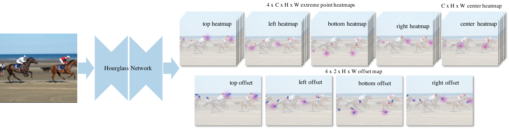
In this paper, we propose ExtremeNet, a bottom-up object detection framework that detects four extreme points (top-most, left-most, bottom-most, right-most) of an object. We use a state-of-the-art keypoint estimation framework newell2016stacked; Chen_2018_CVPR; xiao2018simple; newell2017associative; cao2017realtime to find extreme points, by predicting four multi-peak heatmaps for each object category. In addition, we use one heatmap per category predicting the object center, as the average of two bounding box edges in both the and dimension. We group extreme points into objects with a purely geometry-based approach. We group four extreme points, one from each map, if and only if their geometric center is predicted in the center heatmap with a score higher than a pre-defined threshold. We enumerate all combinations of extreme point prediction, and select the valid ones. The number of extreme point prediction is usually quite small, for COCO lin2014microsoft , and a brute force algorithm implemented on GPU is sufficient. Figure 2 shows an overview of the proposed method.
We are not the first to use deep keypoint prediction for object detection. CornerNet Law_2018_ECCV predicts two opposing corners of a bounding box. They group corner points into bounding boxes using an associative embedding feature newell2017associative. Our approach differs in two key aspects: keypoint definition and grouping. A corner is another form of bounding box, and suffers many of the issues top-down detection suffers from. A corner often lies outside an object, without strong appearance features. Extreme points, on the other hand, lie on objects, are visually distinguishable, and have consistent local appearance features. For example, the top-most point of human is often the head, and the bottom-most point of a car or airplane will be a wheel. This makes the extreme point detection easier. The second difference to CornerNet is the geometric grouping. Our detection framework is fully appearance-based, without any implicit feature learning. In our experiments, the appearance-based grouping works significantly better.
Our idea is motivated by Papadopoulos et al. papadopoulos2017extreme, who proposed to annotate bounding boxes by clicking the four extreme points. This annotation is roughly four times faster to collect and provides richer information than bounding boxes. Extreme points also have a close connection to object masks. Directly connecting the inflated extreme points offers a more fine-grained object mask than the bounding box. In our experiment, we show that fitting a simple octagon to the extreme points yields a good object mask estimation. Our method can be further combined with Deep Extreme Cut (DEXTR) Man+18, which turns extreme point annotations into a segmentation mask for the indicated object. Directly feeding our extreme point predictions as guidance to DEXTR Man+18 leads to close to state-of-the-art instance segmentation results.
Our proposed method achieves a bounding box AP of on COCO test-dev, out-performing all reported one-stage object detectors lin2018focal; zhang2018single; redmon2018yolov3; Law_2018_ECCV and on-par with sophisticated two-stage detectors. A Pascal VOC pascal-voc-2012; BharathICCV2011 pre-trained DEXTR Man+18 model yields a Mask AP of , without using any COCO mask annotations. Code is available at https://github.com/xingyizhou/ExtremeNet.
2 Related Work
Two-stage object detectors Region-CNN family girshick2014rich; he2014spatial; girshick2015fast; ren2015faster; he2017mask considers object detection as two sequential problems: first propose a (large) set of category-agnostic bounding box candidates, crop them, and use an image classification module to classify the cropped region or region feature. R-CNN girshick2014rich uses selective search uijlings2013selective to generate region proposals and feeds them to an ImageNet classification network. SPP he2014spatial and Fast RCNN girshick2015fast first feed an image through a convolutional network and crop an intermediate feature map to reduce computation. Faster RCNN ren2015faster further replaces region proposals uijlings2013selective with a Region Proposal Network. The detection-by-classification idea is intuitive and keeps the best performance so far dai2016r; Dai_2017_ICCV; peng2017megdet; liu2018path; lin2017feature; zhu2017couplenet; huang2017speed; tychsen2017improving; tychsen2017denet; Jiang_2018_ECCV.
Our method does not require region proposal or region classification. We argue that a region is not a necessary component in object detection. Representing an object by four extreme points is also effective and provides as much information as bounding boxes.
One-stage object detector One-stage object detectors lin2018focal; redmon2016you; liu2016ssd; redmon2017yolo9000; Law_2018_ECCV; wang2017point; shen2017dsod do not have a region cropping module. They can be considered as category-specific region or anchor proposal networks and directly assign a class label to each positive anchor. SSD liu2016ssd; fu2017dssd uses different scale anchors in different network layers. YOLOv2 redmon2017yolo9000 learns anchor shape priors. RetinaNet lin2018focal proposes a focal loss to balance the training contribution between positive and negative anchors. RefineDet zhang2018single learns to early reject negative anchors. Well-designed single-stage object detectors achieve very close performance with two-stage ones at higher efficiency.
Our method falls in the one-stage detector category. However, instead of setting anchors in an space, we detects five individual parts (four extreme points and one center) of a bounding box in space. Instead of setting default scales or aspect-ratios as anchors at each pixel location, we only predict the probability for that location being a keypoint. Our center map can also be seen as a scale and aspect ratio agnostic region proposal network without bounding box regression.
Deformable Part Model As a bottom-up object detection method, our idea of grouping center and extreme points is related to Deformable Part Model felzenszwalb2010object. Our center point detector functions similarly with the root filter in DPM felzenszwalb2010object, and our four extreme points can be considered as a universal part decomposition for all categories. Instead of learning the part configuration, our predicted center and four extreme points have a fixed geometry structure. And we use a state-of-the-art keypoint detection network instead of low-level image filters for part detection.
Grouping in bottom-up human pose estimation Determining which keypoints are from the same person is an important component in bottom-up multi-person pose estimation. There are multiple solutions: Newell et al. newell2017associative proposes to learn an associative feature for each keypoint, which is trained using an embedding loss. Cao et al. cao2017realtime learns an affinity field which resembles the edge between connected keypoints. Papandreous et al. papandreou2018personlab learns the displacement to the parent joint on the human skeleton tree, as a 2-d feature for each keypoint. Nie et al. nie2018ppn also learn a feature as the offset with respect to the object center.
In contrast to all the above methods, our center grouping is pure appearance-based and is easy to learn, by exploiting the geometric structure of extreme points and their center.
Implicit keypoint detection Prevalent keypoint detection methods work on well-defined semantic keypoints, e.g., human joints. StarMap zhou2018starmap mixes all types of keypoints using a single heatmap for general keypoint detection. Our extreme and center points are a kind of such general implicit keypoints, but with more explicit geometry property.
3 Preliminaries
Extreme and center points
Let denote the four sides of a bounding box. To annotate a bounding box, a user commonly clicks on the top-left and bottom-right corners. As both points regularly lie outside an object, these clicks are often inaccuracy and need to be adjusted a few times. The whole process takes seconds on average su2012crowdsourcing. Papadopoulos et al. papadopoulos2017extreme propose to annotate the bounding box by clicking the four extreme points , , , , where the box is . An extreme point is a point such that no other point on the object lies further along one of the four cardinal directions : top, bottom, left, right. Extreme click annotation time is 7.2 seconds on average papadopoulos2017extreme. The resulting annotation is on-par with the more time-consuming box annotation. Here, we use the extreme click annotations directly and bypass the bounding box. We additionally use the center point of each object as .
Keypoint detection
Keypoint estimation, e.g., human joint estimation newell2017associative; cao2017realtime; Chen_2018_CVPR; xiao2018simple; he2017mask or chair corner point estimation zhou2018starmap; pavlakos20176, commonly uses a fully convolutional encoder-decoder network to predict a multi-channel heatmap for each type of keypoint (e.g., one heatmap for human head, another heatmap for human wrist). The network is trained in a fully supervised way, with either an L2 loss to a rendered Gaussian map newell2017associative; cao2017realtime; Chen_2018_CVPR; xiao2018simple or with a per-pixel logistic regression loss papandreou2017towards; papandreou2018personlab; Law_2018_ECCV. State-of-the-art keypoint estimation networks, e.g., 104-layer HourglassNet newell2016stacked; Law_2018_ECCV, are trained in a fully convolutional manner. They regress to a heatmap of width and height for each output channel. The training is guided by a multi-peak Gaussian heatmap , where each keypoint defines the mean of a Gaussian Kernel. The standard deviation is either fixed, or set proportional to the object size Law_2018_ECCV. The Gaussian heatmap serves as the regression target in the L2 loss case or as the weight map to reduce penalty near a positive location in the logistic regression case Law_2018_ECCV.
CornerNet
CornerNet Law_2018_ECCV uses keypoint estimation with an HourglassNet newell2016stacked as an object detector. They predict two sets of heatmaps for the opposing corners of the box. In order to balance the positive and negative locations they use a modified focal loss lin2018focal for training:
| (1) |
where and are hyper-parameters and fixed to and during training. is the number of objects in the image.
For sub-pixel accuracy of extreme points, CornerNet additionally regresses to category-agnostic keypoint offset for each corner. This regression recovers part of the information lost in the down-sampling of the hourglass network. The offset map is trained with smooth L1 Loss girshick2015fast on ground truth extreme point locations:
| (2) |
where is the down-sampling factor ( for HourglassNet), is the coordinate of the keypoint.
CornerNet then groups opposing corners into detection using an associative embedding newell2017associative. Our extreme point estimation uses the CornerNet architecture and loss, but not the associative embedding.
Deep Extreme Cut
Deep Extreme Cut (DEXTR) Man+18 is an extreme point guided image segmentation method. It takes four extreme points and the cropped image region surrounding the bounding box spanned by the extreme points as input. From this it produces a category-agnostic foreground segmentation of the indicated object using the semantic segmentation network of Chen et al. chen2018deeplab. The network learns to generate the segmentation mask that matches the input extreme point.
4 ExtremeNet for Object detection
ExtremeNet uses an HourglassNet newell2016stacked to detect five keypoints per class (four extreme points, and one center). We follow the training setup, loss and offset prediction of CornerNet Law_2018_ECCV. The offset prediction is category-agnostic, but extreme-point specific. There is no offset prediction for the center map. The output of our network is thus heatmaps and offset maps, where is the number of classes ( for MS COCO lin2014microsoft). Figure 3 shows an overview. Once the extreme points are extracted, we group them into detections in a purely geometric manner.
4.1 Center Grouping
// are sets of points.
for , , , do
if and then
// If the center is detected
if then
Extreme points lie on different sides of an object. This complicates grouping. For example, an associative embedding newell2017associative might not have a global enough view to group these keypoints. Here, we take a different approach that exploits the spread out nature of extreme points.
The input to our grouping algorithm is five heatmaps per class: one center heatmap and four extreme heatmaps , , , for the top, left, bottom, right, respectively. Given a heatmap, we extract the corresponding keypoints by detecting all peaks. A peak is any pixel location with a value greater than , that is locally maximal in a window surrounding the pixel. We name this procedure as ExtrectPeak.
Given four extreme points , , , extracted from heatmaps , , , , we compute their geometric center . If this center is predicted with a high response in the center map , we commit the extreme points as a valid detection: for a threshold . We then enumerate over all quadruples of keypoints , , , in a brute force manner. We extract detections for each class independently. Algorithm 1 summarizes this procedure. We set and in all experiments.
This brute force grouping algorithm has a runtime of , where is the number of extracted extreme points for each cardinal direction. Supplementary material presents a algorithm that is faster on paper. However, then it is harder to accelerate on a GPU and slower in practice for the MS COCO dataset, where .
4.2 Ghost box suppression
Center grouping may give a high-confidence false-positive detection for three equally spaced colinear objects of the same size. The center object has two choices here, commit to the correct small box, or predict a much larger box containing the extreme points of its neighbors. We call these false-positive detections “ghost” boxes. As we’ll show in our experiments, these ghost boxes are infrequent, but nonetheless a consistent error mode of our grouping.
We present a simple post-processing step to remove ghost boxes. By definition a ghost box contains many other smaller detections. To discourage ghost boxes, we use a form of soft non-maxima suppression bodla2017soft. If the sum of scores of all boxes contained in a certain bounding box exceeds times of the score of itself, we divide its score by . This non-maxima suppression is similar to the standard overlap-based non-maxima suppression, but penalizes potential ghost boxes instead of multiple overlapping boxes.
4.3 Edge aggregation


Extreme points are not always uniquely defined. If vertical or horizontal edges of an object form the extreme points (e.g., the top of a car) any point along that edge might be considered an extreme point. As a result, our network produces a weak response along any aligned edges of the object, instead of a single strong peak response. This weak response has two issues: First, the weaker response might be below our peak selection threshold , and we will miss the extreme point entirely. Second, even if we detect the keypoint, its score will be lower than a slightly rotated object with a strong peak response.
We use edge aggregation to address this issue. For each extreme point, extracted as a local maximum, we aggregate its score in either the vertical direction, for left and right extreme points, or the horizontal direction, for top and bottom keypoints. We aggregate all monotonically decreasing scores, and stop the aggregation at a local minimum along the aggregation direction. Specifically, let be an extreme point and be the vertical or horizontal line segment at that point. Let and be the two closest local minima and . Edge aggregation updates the keypoint score as , where is the aggregation weight. In our experiments, we set . See Fig. 4 for en example.
4.4 Extreme Instance Segmentation
Extreme points carry considerable more information about an object, than a simple bounding box, with at least twice as many annotated values (8 vs 4). We propose a simple method to approximate the object mask using extreme points by creating an octagon whose edges are centered on the extreme points. Specifically, for an extreme point, we extend it in both directions on its corresponding edge to a segment of of the entire edge length. The segment is truncated when it meets a corner. We then connect the end points of the four segments to form the octagon. See Figure 1 for an example.
To further refine the bounding box segmentation, we use Deep Extreme Cut (DEXTR) Man+18, a deep network trained to convert the manually provided extreme points into instance segmentation mask. In this work, we simply replace the manual input of DEXTR Man+18 with our extreme point prediction, to perform a 2-stage instance segmentation. Specifically, for each of our predicted bounding box , we crop the bounding box region, render a Gaussian map with our predicted extreme point, and then feed the concatenated image to the pre-trained DEXTR model. DEXTR Man+18 is class-agnostic, thus we directly use the detected class and score of ExtremeNet. No further post-processing is used.
5 Experiments
We evaluate our method on the popular MS COCO dataset lin2014microsoft. COCO contains rich bounding box and instance segmentation annotations for 80 categories. We train on the train2017 split, which contains 118k images and 860k annotated objects. We perform all ablation studies on val2017 split, with 5k images and 36k objects, and compare to prior work on the test-dev split with contains 20k images The main evaluation metric is average precision over a dense set of fixed recall threshold We show average precision at IOU threshold (), (), and averaged over all thresholds between and (). We also report AP for small, median and large objects (, , ). The test evaluation is done on the official evaluation server. Qualitative results are shown in Table. 4 and can be found more in the supplementary material.
5.1 Extreme point annotations
There are no direct extreme point annotation in the COCO lin2014microsoft. However, there are complete annotations for object segmentation masks. We thus find extreme points as extrema in the polygonal mask annotations. In cases where an edge is parallel to an axis or within a angle, we place the extreme point at the center of the edge. Although our training data is derived from the more expensive segmentation annotation, the extreme point data itself is cheaper to collect than the standard bounding box papadopoulos2017extreme.
5.2 Training details
Our implementation is based on the public implementation of CornerNet Law_2018_ECCV. We strictly follow CornerNets hyper-parameters: we set the input resolution to and output resolution to . Data augmentation consists of flipping, random scaling between and , random cropping, and random color jittering. The network is optimized with Adam kingma2014adam with learning rate . CornerNet Law_2018_ECCV was originally trained on 10 GPUs for 500k iterations, and an equivalent of over GPU days. Due to limited GPU resources, the self-comparison experiments (Table. 1) are finetuned from a pre-trained CornerNet model with randomly initialized head layers on 5 GPUs for iterations with a batch size of 24. Learning rate is dropped at the iteration. The state-of-the-art comparison experiment is trained from scratch on 5 GPUs for iterations with learning rate dropped at the iteration.
5.3 Testing details
For each input image, our network produces four -channel heatmaps for extreme points, one -channel heatmap for center points, and four -channel offset maps. We apply edge aggregation (Section. 4) to each extreme point heatmap, and multiply the center heatmap by to correct for the overall scale change. We then apply the center grouping algorithm (Section. 4.1) to the heatmaps. At most top points are extracted in ExtrectPeak to keep the enumerating efficiency. The predicted bounding box coordinates are refined by adding an offset at the corresponding location of offsetmaps.
Following CornerNet Law_2018_ECCV, we keep the original image resolution instead of resizing it to a fixed size. We use flip augmentation for testing. In our main comparison, we use additional multi-scale (0.5, 0.75, 1, 1.25, 1.5) augmentation. Finally, Soft-NMS bodla2017soft filters all augmented detection results. Testing on one image takes 322ms (3.1FPS), with 168ms on network forwarding, 130ms on decoding and rest time on image pre- and post-processing (NMS).
5.4 Ablation studies
| 40.3 | 55.1 | 43.7 | 21.6 | 44.0 | 56.1 | |
| w/ multi-scale testing | 43.3 | 59.6 | 46.8 | 25.7 | 46.6 | 59.4 |
| w/o Center grouping | 38.2 | 53.8 | 40.4 | 20.6 | 41.5 | 52.9 |
| w/o Edge aggregation | 39.6 | 54.7 | 43.0 | 22.0 | 43.0 | 54.1 |
| w/o Ghost removal | 40.0 | 54.7 | 43.3 | 21.6 | 44.2 | 54.1 |
| w/ gt center | 48.6 | 62.1 | 53.9 | 26.3 | 53.7 | 66.7 |
| w/ gt extreme | 56.3 | 67.2 | 60.0 | 40.9 | 62.0s | 64.0 |
| w/ gt extreme + center | 79.8 | 94.5 | 86.2 | 65.5 | 88.7 | 95.5 |
| w/ gt ex. + ct. + offset | 86.0 | 94.0 | 91.3 | 73.4 | 95.7 | 98.4 |
| Backbone | Input resolution | |||||||
|---|---|---|---|---|---|---|---|---|
| Two-stage detectors | ||||||||
| Faster R-CNN w/ FPN lin2017feature | ResNet-101 | 36.2 | 59.1 | 39.0 | 18.2 | 39.0 | 48.2 | |
| Deformable-CNN Dai_2017_ICCV | Inception-ResNet | 37.5 | 58.0 | - | 19.4 | 40.1 | 52.5 | |
| Deep Regionlets Xu_2018_ECCV | ResNet-101 | 39.3 | 59.8 | - | 21.7 | 43.7 | 50.9 | |
| Mask R-CNN he2017mask | ResNeXt-101 | 39.8 | 62.3 | 43.4 | 22.1 | 43.2 | 51.2 | |
| LH R-CNN li2017light | ResNet-101 | 41.5 | - | - | 25.2 | 45.3 | 53.1 | |
| Cascade R-CNN cai2017cascade | ResNet-101 | 42.8 | 62.1 | 46.3 | 23.7 | 45.5 | 55.2 | |
| D-RFCN + SNIP singh2018analysis | DPN-98 | 45.7 | 67.3 | 51.1 | 29.3 | 48.8 | 57.1 | |
| PANet liu2018path | ResNeXt-101 | 47.4 | 67.2 | 51.8 | 30.1 | 51.7 | 60.0 | |
| One-stage detectors | ||||||||
| YOLOv2 redmon2017yolo9000 | DarkNet-19 | 21.6 | 44.0 | 19.2 | 5.0 | 22.4 | 35.5 | |
| YOLOv3 redmon2018yolov3 | DarkNet-53 | 33.0 | 57.9 | 34.4 | 18.3 | 35.4 | 41.9 | |
| SSD liu2016ssd | ResNet-101 | 31.2 | 50.4 | 33.3 | 10.2 | 34.5 | 49.8 | |
| DSSD fu2017dssd | ResNet-101 | 33.2 | 53.3 | 35.2 | 13.0 | 35.4 | 51.1 | |
| RetinaNet lin2018focal | ResNet-101 | 39.1 | 59.1 | 42.3 | 21.8 | 42.7 | 50.2 | |
| RefineDet (SS) zhang2018single | ResNet-101 | 36.4 | 57.5 | 39.5 | 16.6 | 39.9 | 51.4 | |
| RefineDet (MS) zhang2018single | ResNet-101 | 41.8 | 62.9 | 45.7 | 25.6 | 45.1 | 54.1 | |
| CornerNet (SS) Law_2018_ECCV | Hourglass-104 | 40.5 | 56.5 | 43.1 | 19.4 | 42.7 | 53.9 | |
| CornerNet (MS) Law_2018_ECCV | Hourglass-104 | 42.1 | 57.8 | 45.3 | 20.8 | 44.8 | 56.7 | |
| ExtremeNet (SS) | Hourglass-104 | 40.2 | 55.5 | 43.2 | 20.4 | 43.2 | 53.1 | |
| ExtremeNet (MS) | Hourglass-104 | 43.7 | 60.5 | 47.0 | 24.1 | 46.9 | 57.6 | |
| BBox | 12.1 | 34.9 | 6.2 | 8.2 | 12.7 | 16.9 |
|---|---|---|---|---|---|---|
| Ours octagon | 18.9 | 44.5 | 13.7 | 10.4 | 20.4 | 28.3 |
| Ours+DEXTR Man+18 | 34.6 | 54.9 | 36.6 | 16.6 | 36.5 | 52.0 |
| Mask RCNN-50 he2017mask | 34.0 | 55.5 | 36.1 | 14.4 | 36.7 | 51.9 |
| Mask RCNN-101 he2017mask | 37.5 | 60.6 | 39.9 | 17.7 | 41.0 | 55.4 |
| Extreme point heatmap | Center heatmap | Octagon mask | Extreme points+DEXTR Man+18 |
|---|---|---|---|
![[Uncaptioned image]](1901.08043v3/qualitative/712_ex.png) |
![[Uncaptioned image]](1901.08043v3/qualitative/712_ct.png) |
![[Uncaptioned image]](1901.08043v3/qualitative/712_oct.png) |
![[Uncaptioned image]](1901.08043v3/qualitative/712_mask.png) |
![[Uncaptioned image]](1901.08043v3/qualitative/816_ex.png) |
![[Uncaptioned image]](1901.08043v3/qualitative/816_ct.png) |
![[Uncaptioned image]](1901.08043v3/qualitative/816_oct.png) |
![[Uncaptioned image]](1901.08043v3/qualitative/816_mask.png) |
![[Uncaptioned image]](1901.08043v3/qualitative/934_ex.png) |
![[Uncaptioned image]](1901.08043v3/qualitative/934_ct.png) |
![[Uncaptioned image]](1901.08043v3/qualitative/934_oct.png) |
![[Uncaptioned image]](1901.08043v3/qualitative/934_mask.png) |
![[Uncaptioned image]](1901.08043v3/qualitative/581_ex.png) |
![[Uncaptioned image]](1901.08043v3/qualitative/581_ct.png) |
![[Uncaptioned image]](1901.08043v3/qualitative/581_oct.png) |
![[Uncaptioned image]](1901.08043v3/qualitative/581_mask.png) |
Center Grouping vs. Associative Embedding
Our ExtremeNet can also be trained with an Associative Embedding newell2017associative similar to CornerNet Law_2018_ECCV, instead of our geometric center point grouping. We tried this idea and replaced the center map with a four-channel associative embedding feature map trained with a Hinge Loss Law_2018_ECCV. Table 1 shows the result. We observe a AP drop when using the associative embedding. While associative embeddings work well for human pose estimation and CornerNet, our extreme points lie on the very side of objects. Learning the identity and appearance of entire objects from the vantage point of its extreme points might simply be too hard. While it might work well for small objects, where the entire object easily fits into the effective receptive field of a keypoint, it fails for medium and large objects as shown in Table 1. Furthermore, extreme points often lie at the intersection between overlapping objects, which further confuses the identity feature. Our geometric grouping method gracefully deals with these issues, as it only needs to reason about appearance.
Edge aggregation
Edge aggregation (Section 4) gives a decent AP improvement of . It proofs more effective for larger objects, that are more likely to have a long axis aligned edges without a single well defined extreme point. Removing edge aggregation improves the decoding time to 76ms and overall speed to 4.1 FPS.
Ghost box suppression
Our simple ghost bounding box suppression (Section 4.2) yields AP improvement. This suggests that ghost boxes are not a significant practical issue in MS COCO. A more sophisticated false-positive removal algorithm, e.g., learn NMS hosang2017learning, might yield a slightly better result.
Error Analysis
To better understand where the error comes from and how well each of our components is trained, we provide error analysis by replacing each output component with its ground truth. Table 1 shows the result. A ground truth center heatmap alone does not increase AP much. This indicates that our center heatmap is trained quite well, and shows that the implicit object center is learnable. Replacing the extreme point heatmap with ground truth gives AP improvement. When replacing both extreme point heatmap and center heatmap, the result comes to , much higher than replacing one of them. This is due to that our center grouping is very strict in the keypoint location and a high performance requires to improve both extreme point heatmap and center heatmap. Adding the ground truth offsets further increases the AP to . The rest error is from the ghost box (Section 4.2).
5.5 State-of-the-art comparisons
Table 2 compares ExtremeNet to other state-of-the-art methods on COCO test-dev. Our model with multi-scale testing achieves an AP of , outperforming all reported one-stage object detectors and on-par with popular two-stage detectors. Notable, it performs higher than CornerNet, which shows the advantage of detecting extreme and center points over detecting corners with associative features. In single scale setting, our performance is AP below CornerNet Law_2018_ECCV. However, our method has higher AP for small and median objects than CornerNet, which is known to be more challenging. For larger objects our center response map might not be accurate enough to perform well, as a few pixel shift might make the difference between a detection and a false-negative. Further, note that we used the half number of GPUs to train our model.
5.6 Instance Segmentation
Finally, we compare our instance segmentation results with/ without DEXTR Man+18 to other baselines in Table 3.
As a dummy baseline, we directly assign all pixels inside the rectangular bounding box as the segmentation mask. The result on our best-model (with bounding box AP) is Mask AP. The simple octagon mask (Section. 4.4) based on our predicted extreme points gets a mask AP of , much better than the bounding box baseline. This shows that this simple octagon mask can give a relatively reasonable object mask without additional cost. Note that directly using the quadrangle of the four extreme points yields a too-small mask, with a lower IoU.
When combined with DEXTR Man+18, our method achieves a mask AP of on COCO val2017. To put this result in a context, the state-of-the-art Mask RCNN he2017mask gets a mask AP of with ResNeXt-101-FPN lin2017feature; xie2017aggregated backbone and AP with Res50-FPN. Considering the fact that our model has not been trained on the COCO segmentation annotation, or any class specific segmentations at all, our result which is on-par with Res50 he2016deep and AP below ResNeXt-101 is very competitive.
6 Conclusion
In conclusion, we present a novel object detection framework based on bottom-up extreme points estimation. Our framework extracts four extreme points and groups them in a purely geometric manner. The presented framework yields state-of-the-art detection results and produces competitive instance segmentation results on MSCOCO, without seeing any COCO training instance segmentations.
Acknowledgement
We thank Chao-Yuan Wu, Dian Chen, and Chia-Wen Cheng for helpful feedback.
References
- (1) N. Bodla, B. Singh, R. Chellappa, and L. S. Davis. Soft-nms—improving object detection with one line of code. In ICCV, 2017.
- (2) Z. Cai and N. Vasconcelos. Cascade r-cnn: Delving into high quality object detection. CVPR, 2018.
- (3) Z. Cao, T. Simon, S.-E. Wei, and Y. Sheikh. Realtime multi-person 2d pose estimation using part affinity fields. In CVPR, 2017.
- (4) L.-C. Chen, G. Papandreou, I. Kokkinos, K. Murphy, and A. L. Yuille. Deeplab: Semantic image segmentation with deep convolutional nets, atrous convolution, and fully connected crfs. PAMI, 2018.
- (5) Y. Chen, Z. Wang, Y. Peng, Z. Zhang, G. Yu, and J. Sun. Cascaded pyramid network for multi-person pose estimation. In CVPR, 2018.
- (6) J. Dai, Y. Li, K. He, and J. Sun. R-fcn: Object detection via region-based fully convolutional networks. In NIPS, 2016.
- (7) J. Dai, H. Qi, Y. Xiong, Y. Li, G. Zhang, H. Hu, and Y. Wei. Deformable convolutional networks. In ICCV, 2017.
- (8) M. Everingham, L. Van Gool, C. K. I. Williams, J. Winn, and A. Zisserman. The PASCAL Visual Object Classes Challenge 2012 (VOC2012) Results. http://www.pascal-network.org/challenges/VOC/voc2012/workshop/index.html.
- (9) P. F. Felzenszwalb, R. B. Girshick, D. McAllester, and D. Ramanan. Object detection with discriminatively trained part-based models. PAMI, 2010.
- (10) C.-Y. Fu, W. Liu, A. Ranga, A. Tyagi, and A. C. Berg. Dssd: Deconvolutional single shot detector. arXiv preprint, 2017.
- (11) R. Girshick. Fast r-cnn. In ICCV, 2015.
- (12) R. Girshick, J. Donahue, T. Darrell, and J. Malik. Rich feature hierarchies for accurate object detection and semantic segmentation. In CVPR, 2014.
- (13) R. B. Girshick, P. F. Felzenszwalb, and D. A. Mcallester. Object detection with grammar models. In NIPS, 2011.
- (14) B. Hariharan, P. Arbelaez, L. Bourdev, S. Maji, and J. Malik. Semantic contours from inverse detectors. In ICCV, 2011.
- (15) K. He, G. Gkioxari, P. Dollár, and R. Girshick. Mask r-cnn. In ICCV, 2017.
- (16) K. He, X. Zhang, S. Ren, and J. Sun. Spatial pyramid pooling in deep convolutional networks for visual recognition. In ECCV, 2014.
- (17) K. He, X. Zhang, S. Ren, and J. Sun. Deep residual learning for image recognition. In CVPR, 2016.
- (18) J. H. Hosang, R. Benenson, and B. Schiele. Learning non-maximum suppression. In CVPR, 2017.
- (19) J. Huang, V. Rathod, C. Sun, M. Zhu, A. Korattikara, A. Fathi, I. Fischer, Z. Wojna, Y. Song, S. Guadarrama, et al. Speed/accuracy trade-offs for modern convolutional object detectors. In CVPR, 2017.
- (20) B. Jiang, R. Luo, J. Mao, T. Xiao, and Y. Jiang. Acquisition of localization confidence for accurate object detection. In ECCV, September 2018.
- (21) D. P. Kingma and J. Ba. Adam: A method for stochastic optimization. ICLR, 2014.
- (22) H. Law and J. Deng. Cornernet: Detecting objects as paired keypoints. In ECCV, 2018.
- (23) Z. Li, C. Peng, G. Yu, X. Zhang, Y. Deng, and J. Sun. Light-head r-cnn: In defense of two-stage object detector. arXiv preprint, 2017.
- (24) T.-Y. Lin, P. Dollár, R. B. Girshick, K. He, B. Hariharan, and S. J. Belongie. Feature pyramid networks for object detection. In CVPR, 2017.
- (25) T.-Y. Lin, P. Goyal, R. Girshick, K. He, and P. Dollár. Focal loss for dense object detection. ICCV, 2017.
- (26) T.-Y. Lin, M. Maire, S. Belongie, J. Hays, P. Perona, D. Ramanan, P. Dollár, and C. L. Zitnick. Microsoft coco: Common objects in context. In ECCV, 2014.
- (27) S. Liu, L. Qi, H. Qin, J. Shi, and J. Jia. Path aggregation network for instance segmentation. In CVPR, 2018.
- (28) W. Liu, D. Anguelov, D. Erhan, C. Szegedy, S. Reed, C.-Y. Fu, and A. C. Berg. Ssd: Single shot multibox detector. In ECCV, 2016.
- (29) K. Maninis, S. Caelles, J. Pont-Tuset, and L. Van Gool. Deep extreme cut: From extreme points to object segmentation. In CVPR, 2018.
- (30) A. Newell, Z. Huang, and J. Deng. Associative embedding: End-to-end learning for joint detection and grouping. In NIPS, 2017.
- (31) A. Newell, K. Yang, and J. Deng. Stacked hourglass networks for human pose estimation. In ECCV, 2016.
- (32) X. Nie, J. Feng, J. Xing, and S. Yan. Pose partition networks for multi-person pose estimation. In ECCV, 2018.
- (33) D. P. Papadopoulos, J. R. Uijlings, F. Keller, and V. Ferrari. Extreme clicking for efficient object annotation. In ICCV, 2017.
- (34) G. Papandreou, T. Zhu, L.-C. Chen, S. Gidaris, J. Tompson, and K. Murphy. Personlab: Person pose estimation and instance segmentation with a bottom-up, part-based, geometric embedding model. ECCV, 2018.
- (35) G. Papandreou, T. Zhu, N. Kanazawa, A. Toshev, J. Tompson, C. Bregler, and K. Murphy. Towards accurate multi-person pose estimation in the wild. In CVPR, 2017.
- (36) G. Pavlakos, X. Zhou, A. Chan, K. G. Derpanis, and K. Daniilidis. 6-dof object pose from semantic keypoints. In ICRA, 2017.
- (37) C. Peng, T. Xiao, Z. Li, Y. Jiang, X. Zhang, K. Jia, G. Yu, and J. Sun. Megdet: A large mini-batch object detector. CVPR, 2018.
- (38) J. Redmon, S. Divvala, R. Girshick, and A. Farhadi. You only look once: Unified, real-time object detection. In CVPR, 2016.
- (39) J. Redmon and A. Farhadi. Yolo9000: better, faster, stronger. CVPR, 2017.
- (40) J. Redmon and A. Farhadi. Yolov3: An incremental improvement. arXiv preprint, 2018.
- (41) S. Ren, K. He, R. Girshick, and J. Sun. Faster r-cnn: Towards real-time object detection with region proposal networks. In NIPS, 2015.
- (42) Z. Shen, Z. Liu, J. Li, Y.-G. Jiang, Y. Chen, and X. Xue. Dsod: Learning deeply supervised object detectors from scratch. In ICCV, 2017.
- (43) B. Singh and L. S. Davis. An analysis of scale invariance in object detection–snip. In CVPR, 2018.
- (44) H. Su, J. Deng, and L. Fei-Fei. Crowdsourcing annotations for visual object detection. In AAAIW, 2012.
- (45) L. Tychsen-Smith and L. Petersson. Denet: Scalable real-time object detection with directed sparse sampling. arXiv preprint arXiv:1703.10295, 2017.
- (46) L. Tychsen-Smith and L. Petersson. Improving object localization with fitness nms and bounded iou loss. CVPR, 2017.
- (47) J. R. Uijlings, K. E. Van De Sande, T. Gevers, and A. W. Smeulders. Selective search for object recognition. IJCV, 2013.
- (48) X. Wang, K. Chen, Z. Huang, C. Yao, and W. Liu. Point linking network for object detection. arXiv preprint arXiv:1706.03646, 2017.
- (49) B. Xiao, H. Wu, and Y. Wei. Simple baselines for human pose estimation and tracking. In ECCV, 2018.
- (50) S. Xie, R. Girshick, P. Dollár, Z. Tu, and K. He. Aggregated residual transformations for deep neural networks. In CVPR, 2017.
- (51) H. Xu, X. Lv, X. Wang, Z. Ren, N. Bodla, and R. Chellappa. Deep regionlets for object detection. In ECCV, 2018.
- (52) S. Zhang, L. Wen, X. Bian, Z. Lei, and S. Z. Li. Single-shot refinement neural network for object detection. In CVPR, 2018.
- (53) X. Zhou, A. Karpur, L. Luo, and Q. Huang. Starmap for category-agnostic keypoint and viewpoint estimation. In ECCV, 2018.
- (54) Y. Zhu, C. Zhao, J. Wang, X. Zhao, Y. Wu, H. Lu, et al. Couplenet: Coupling global structure with local parts for object detection. In ICCV, 2017.