The future is not always openThanks: This work was supported by research grant P28770 of the Austrian Science Fund FWF, and WTZ Project No. CZ 12/2018 of OeAD
Abstract.
We demonstrate the breakdown of several fundamentals of Lorentzian causality theory in low regularity. Most notably, chronological futures (defined naturally using locally Lipschitz curves) may be non-open, and may differ from the corresponding sets defined via piecewise -curves. By refining the notion of a causal bubble from [CG12], we characterize spacetimes for which such phenomena can occur, and also relate these to the possibility of deforming causal curves of positive length into timelike curves (push-up). The phenomena described here are, in particular, relevant for recent synthetic approaches to low regularity Lorentzian geometry where, in the absence of a differentiable structure, causality has to be based on locally Lipschitz curves.
Key words and phrases:
Causality theory, low regularity, chronological future, causal bubbles2010 Mathematics Subject Classification
53C50; 83C751. Introduction
Until a decade ago Lorentzian causality theory had mostly been studied under the assumption of a smooth spacetime metric. However, with the analytic viewpoint on general relativity becoming more and more prevalent, issues of regularity have increasingly come to the fore. In particular, while the geometric core of the theory is traditionally formulated in the smooth category, the analysis of the initial value problem, for example, requires one to consider metrics of low regularity.
Beginning in 2011 with the independent works of [FS12] and [CG12], a systematic study of Lorentzian causality theory under low regularity assumptions began and has brought to light several, sometimes surprising, facts. In a nutshell, while some features of causality theory are rather robust and topological in nature, other results are usually proved by local arguments involving geodesically convex neighbourhoods, which do exist for -metrics [Min15, KSS14]. Consequently for this regularity class the bulk of causality theory [CG12, Min15, KSSV14] including the singularity theorems [KSSV15, KSV15, GGKS18] remains valid. Moreover, arguments from causality theory which neither explicitly involve the exponential map nor geodesics have been found to extend to locally Lipschitz metrics, see [CG12, Thm. 1.25], [Min19, Rem. 2.5]. However, below , explicit counterexamples show that convex neighbourhoods may no longer exist for metrics of Hölder regularity for any [HW51, SS18].
Moreover, Lorentzian causality theory has been generalized to a theory of cone structures, i.e., set-valued maps that assign a cone in the tangent space to each point on a manifold. This setting allows one to develop those aspects of the theory that merely depend on topological arguments under weak regularity assumptions. At the same time, this has led to the introduction of new methods to the field: Using weak KAM theory, existence results for smooth time functions have been derived for -cone structures in [FS12, Fat15], while in [BS18] dynamical systems theory has been employed to derive similar results for merely upper semi-continuous cone structures. In a landmark paper [Min19], Minguzzi has extended these studies using methods from set-valued analysis, convexity and order topology to develop large parts of causality theory for locally Lipschitz cone structures.
Returning to the metric spacetime setting, some results, such as the Avez–Seifert theorem, have been extended to -Lorentzian metrics [Säm16]. Moreover, a number of fundamental works on the -extendibility of spacetimes [Sbi18a, Sbi18b, GLS18] have appeared recently. However, already in [CG12] it was observed that two key features of causality may fail for metrics of regularity below Lipschitz:
- (1)
The push up principle, i.e., , may cease to hold11 1 Here and denote the chronological and the causal relation, respectively, and e.g. with and .;
- (2)
Light cones may cease to be hypersurfaces as they “bubble up” to have a nonempty interior.
Moreover, some fundamental questions raised in [CG12] remained open, especially the openness of the chronological future of a point . In this paper, we answer this question (in the negative) and clarify its relation to points (1) and (2) above. This leads to a number of natural questions concerning the relation between causal and timelike futures and pasts when defined using various classes of curves (like Lipschitz or piecewise ). To answer these, we construct several counterexamples that exhibit a further breakdown of standard causality properties beyond those already investigated in [CG12].
Classical accounts on causality theory mainly use piecewise -curves.
It has to be noted, however, that limit curve theorems, which form a
fundamental tool in causality theory, fail to respect this regularity class. This has
led Chruściel in [Chr11] to base smooth causality theory entirely on
the class of locally Lipschitz curves, an approach that has been adopted in most
of the subsequent studies in low regularity. In fact, Chruściel put it as follows in [Chr11, p. 14]:
“In previous treatments of causality theory [BEE96, Ger70, HE73, O’N83, Pen72, Wal84] one defines future
directed timelike paths as those paths which are piecewise differentiable, with timelike and future
directed wherever defined; at break points one further assumes that both the left-sided and right-sided derivatives are
timelike. This definition turns out to be quite inconvenient for several purposes. For instance, when studying
the global causal structure of space-times one needs to take limits of timelike curves,
obtaining thus — by definition — causal future directed paths. Such limits will
not be piecewise differentiable most of the time, which leads one to the necessity
of considering paths with poorer differentiability properties. One then faces the
unhandy situation in which timelike and causal paths have completely different
properties. In several theorems separate proofs have then to be given. The approach
we present avoids this, leading — we believe — to a considerable simplification of
the conceptual structure of the theory.”
Besides the above, a strong reason for basing causality theory entirely on locally Lipschitz curves comes from the desire to develop synthetic methods in Lorentzian geometry. In fact, following the pioneering works [Har82, AB08], recently methods from synthetic geometry and, in particular, length spaces have been implemented in the Lorentzian setting and in causality theory [KS18, GKS19]. In this framework, which generalizes low regularity Lorentzian geometry to the level of metric spaces, -curves are not available. Thus one needs a broad enough framework within which to address the problems highlighted by the examples given in Section 3 of the present paper.
This article is structured as follows. In Section 2 we define the basic notions of causality theory in several variants and establish some fundamental relations between them. We then introduce tools tailored to low regularity, which enable us to characterise openness of chronological futures and pasts, relate non-bubbling with push-up and clarify several aspects of pathological behaviour of continuous spacetimes. In Section 3 we provide explicit continuous spacetimes that display various pathologies. In particular, we give for the first time examples where the chronological future is not open and where the chronological future defined via smooth curves and the one defined via Lipschitz curves differ. This answers several open questions raised in [CG12]. The final section provides an overview of the interdependence of the various causality notions studied in this work.
To conclude this introduction we introduce some basic notation. Throughout this paper, will denote a smooth connected second countable Hausdorff manifold. Unless otherwise stated, will be a continuous Lorentzian metric on , and we will assume that is time-oriented (i.e., there exists a continuous timelike vector field , that is, everywhere). We then call a continuous spacetime. We shall also fix a smooth complete Riemannian metric on and denote the induced (length) metric by and the induced norm by . Given Lorentzian metrics , , we say that has strictly wider light cones than , denoted by , if for any tangent vector , implies that (cf. [MS08, Sec. 3.8.2], [CG12, Sec. 1.2]). Thus any -causal vector is timelike for .
2. Curves, bubbles, and open questions
For Lorentzian metrics of regularity at least , chronological futures and pasts are usually defined via piecewise (or )-curves (e.g., [HE73, O’N83, BEE96, MS08]). Especially when working in lower regularity, several authors have employed more general classes of curves, the widest one being that of absolutely continuous curves, basically due to the fact that this is the largest class of functions for which the Fundamental Theorem of Calculus holds. This in turn is required to obtain a reasonable notion of length of curves and to control the curves via their causality. To see this let be the Cantor function (which has bounded variation) and consider the curve in two-dimensional Minkowski spacetime . Then parametrizes the timelike curve , but its tangent is almost everywhere, i.e., spacelike.
Furthermore, absolutely continuous causal curves always possess a locally Lipschitz reparametrisation (cf. Lemma 2.8 below). On the other hand, irrespective of the regularity of the metric, the limit curve theorems ([Min08]), which are of central importance in causality theory, even when applied to families of smooth causal curves typically yield curves that are merely locally Lipschitz continuous. It is therefore natural to define causal futures and pasts using such curves, and indeed it was demonstrated in [Chr11, CG12, Min15, KSSV14] for spacetimes, as well as in the significantly more general setting of cone structures in [FS12, BS18, Min19] that a fully satisfactory causality theory can be based on locally Lipschitz causal curves. As we shall see below, the situation is more involved in the case of timelike curves.
To discuss the dependence of causality theory on the underlying notions of timelike respectively causal curves, we introduce the following notations:
Definition 2.1.
We denote by
- (1)
the set of all absolutely continuous curves from an interval into .
- (2)
the set of all locally Lipschitz curves from an interval into .
- (3)
the set of all piecewise continuously differentiable curves from an interval into .
- (4)
the set of all smooth curves from an interval into .
Here, a curve is called absolutely continuous if its components in any chart are absolutely continuous, or, equivalently, if it is absolutely continuous as a map into the metric space , where we recall that is the metric on induced by the Riemannian metric on (cf. the discussion preceding Thm. 6 in [Min15]).
Clearly, we have
| (2.1) |
Henceforth, when we say that a curve in is in fact an element of one of these smaller classes then we mean that there exists a re-parametrization of that lies in this class.
The definition typically employed in the smooth case (cf. the above references), but sometimes also used for continuous metrics (e.g. in [Sbi18a]), is the following.
Definition 2.2.
Let , then is called
-
timelike if everywhere.
-
causal if and everywhere.
At breakpoints, the understanding is that the above conditions are satisfied for both the one-sided tangents. A causal curve is called future (past) directed if belongs to the future (past) light cone everywhere (at the breakpoints this means that both one-sided tangents belong to the same light cone).
The usual definition of causal curves of regularity below piecewise is as follows (cf. [CG12, Def. 1.3]).
Definition 2.3.
Let , then is called
- (1)
timelike if almost everywhere,
- (2)
causal if and almost everywhere.
A causal curve is called future (past) directed if belongs to the future (past) light cone almost everywhere.
Remark 2.4.
In [BS18], there is one further notion of timelike curve that we should mention: The authors call a Lipschitz curve timelike if its Clarke differential lies in the open chronological cone in the tangent space at each parameter value. They then show ([BS18, Lem. 2.11]) that, using this definition, the chronological futures and pasts of a point are precisely the sets (see Definition 2.5 below). Therefore, there is no need for a separate treatment of this approach.
Henceforth we will adhere to the following convention: Whenever a curve is in we will use Definition 2.3, however if a curve is explicitly noted to be in , then we use Definition 2.2.
We now can define the chronological and causal future and past of a point depending on the class of curves chosen.
Definition 2.5.
Let and let . The chronological and causal future/past of with respect to are
| (2.2) | ||||
| (2.3) |
Moreover, for any subset we set and .
From (2.1) we immediately see that for any we have
| (2.4) | ||||
| (2.5) |
Next we recall some key notions from [CG12] that will be important for our further considerations. For any , let denote the metric on (so is the Minkowski metric).
Definition 2.6.
A chart of centred at is called cylindrical for if is relatively compact, for some interval and open, and
- (i)
, the Minkowski metric.
- (ii)
There exists some such that on .
Note that point (ii) above implies that is timelike and () is spacelike on . By [CG12, Prop. 1.10], every point lies in the domain of a cylindrical chart. Such a domain is called a cylindrical neighbourhood.
Following [CG12, Def. 1.3], an absolutely continuous curve is called locally uniformly timelike (l.u.t.) if there exists a smooth Lorentzian metric such that almost everywhere. For open and , by we denote the set of all points that can be reached by a future (respectively past) directed l.u.t. curve in emanating from . So
(with the chronological future/past of in with respect to the smooth Lorentzian metric and using smooth curves). In particular it follows that is open.
It was shown in the proof of [CG12, Prop. 1.10] that in terms of a cylindrical chart (where we usually will suppress notationally), is given as the graph of a Lipschitz function , that is contained in the epigraph of , and that the interior of , denoted by , equals the strict epigraph of . Here, is defined as the pointwise limit of the (Lipschitz) graphing functions of , where the are smooth Lorentzian metrics converging locally uniformly to as . Moreover, the graphing function of is denoted by .

Lemma 2.7.
For any continuous spacetime and any ,
| (2.6) |
In particular, is open.
Proof.
Clearly, . Conversely, let be a future-directed timelike piecewise curve from to some and set (with the maximum taken over both values at the finitely many breakpoints). Moreover, we have that on for some . By [CG12, Prop. 1.2] there exists a smooth Lorentzian metric such that , where
| (2.7) |
Consequently, for all , so . ∎
The following Lemma is an analogue of [Kri99, Lem. 3.2.1] (providing a distinguished local parametrization for continuous causal curves in smooth spacetimes) for continuous metrics and cylindrical neighbourhoods:
Lemma 2.8.
Let be a continuous spacetime, and let be a cylindrical chart around . Let be an absolutely continuous future directed causal curve. Then there is a reparametrisation of , with strictly increasing and absolutely continuous, such that in the chart , for all one has
| (2.8) |
Proof.
Suppressing notationally, let and on . Then is also future directed with respect to and hence
| (2.9) |
almost everywhere. Thus almost everywhere, and so is strictly monotonically increasing. Setting and observing that almost everywhere, we obtain that is absolutely continuous by a result of Zarecki [Nat55, p. 271]. Consequently, is absolutely continuous by [Nat55, Thm. 3, Ch. IX, §1] and so is a future directed causal curve with (note that absolutely continuous functions map sets of measure zero to sets of measure zero — Lusin’s property, see e.g. [AT04, Thm. 3.4.3]). ∎
The previous result allows us to conclude that absolutely continuous causal curves always possess a reparametrisation that is Lipschitz-continuous. This fact was already noticed in [Min19, Rem. 2.3]. We include an alternative proof based on cylindrical neighbourhoods for convenience.
Lemma 2.9.
Let be a continuous spacetime. Then any causal curve in is locally Lipschitz continuous, hence lies in . Thus, for any , and .
Proof.
Let be an absolutely continuous future directed causal curve and let . Set and let be a cylindrical neighbourhood of . Moreover, let such that and let with on . Without loss of generality we can assume that on by Lemma 2.8. Then is timelike for and hence
| (2.10) |
where denotes the Euclidean norm in the chart. This implies that . Consequently, is bounded and hence is Lipschitz continuous. ∎
Based on this result, for a continuous spacetime we shall henceforth define the chronological respectively causal future/past of a point by and . This is in accordance with the conventions used in, e.g., [Chr11, CG12, FS12, KSSV14, Säm16, GGKS18, GL18, GLS18], and, for the case of also with [BS18, Min15, Min19].
For chronological (i.e., possessing no closed timelike curves) spacetimes we have the following characterization of openness of chronological futures and pasts:
Theorem 2.10.
Let be a continuous and chronological spacetime. Then the following are equivalent:
- (i)
For all , is open.
- (ii)
For all , is achronal.
- (iii)
For all , is an achronal Lipschitz-hypersurface.
- (iv)
If is a future/past set with , then is an achronal Lipschitz-hypersurface.
Proof.
(iii)(ii) is clear.
(ii)(i): Suppose that were not open for some . Then there exists some . As is chronological, . Since clearly , it follows that . But then the elements and of can be connected by a timelike curve, contradicting achronality.
(i)(iv): Using cylindrical neighbourhoods, this follows exactly as in the smooth case (cf., e.g., [O’N83, Cor. 14.27]), cf. also [GL17, Proof of Thm. 2.6]. For a detailed proof see [Lec16, Thm. 2.3.5].
(iv)(iii): One only has to note that each is non-empty, which follows from being chronological, cf. the argument in (ii)(i) above. ∎
The spacetime is called causally plain ([CG12, Def. 1.16]) if every possesses a cylindrical neighbourhood such that . Otherwise it is called bubbling22 2 We note that the phenomenon of bubbling, albeit not under this name, was first observed in [Chr91].. Note that whenever we work in a cylindrical chart, all topological notions (like closure, boundary, interior) refer to the relative topology in . If , then the open and non-empty set ([CG12, Prop. 1.10 (vi)])
is called the future bubble set of (and analogously for the past bubble set), cf. Figure 1. Refining this terminology, we additionally introduce the interior future bubble set
as well as the exterior future bubble set
and analogously for the past.
Using Lemma 2.7 and Lemma 2.9, it follows that consists of those points that can be reached from by a future directed Lipschitz timelike curve, but not by a future directed piecewise timelike curve. It remained an open problem in [CG12] whether spacetimes with non-trivial interior bubble sets actually exist. We will give examples of this phenomenon in the next section.
The exterior bubbling set is closely connected to push-up properties. To relate these to the concepts introduced above, let us first give a formal definition:
Definition 2.11.
A continuous spacetime is said to possess the push-up property if the following holds: Whenever is a (absolutely continuous) future/past directed causal curve from to and if has non-zero Lebesgue measure, then in any neighbourhood of there exists a future/past directed timelike Lipschitz curve connecting and . In particular, respectively .
This property implies all the commonly used versions of push-up results. In particular, for an absolutely continuous causal curve the set exists and is future/past directed timelike has non-zero Lebesgue measure if and only if has positive length. A spacetime that possesses the push-up property in the sense of Definition 2.11 also satisfies what in [Chr11, Lemma 2.4.14] and [CG12, Lemma 1.22] are called push-up Lemma I (i.e., for any ) and push-up Lemma II, cf. [Chr11, Lemma 2.9.10] and [CG12, Lemma 1.24]. The following result shows that push-up is in fact equivalent to the non-existence of exterior bubbling:
Theorem 2.12.
Let be a continuous spacetime. The following are equivalent:
- (i)
For each and each cylindrical chart centred at , .
- (ii)
For each and each cylindrical chart centred at , .
- (iii)
possesses the push-up property.
Proof.
We will use the facts and notations for cylindrical charts introduced prior to Lemma 2.7.
(i)(iii): By covering with cylindrical charts contained in the given neighbourhood of it suffices to show push-up for a curve emanating from that is future-directed causal and such that the set has positive Lebesgue-measure . Moreover, by Lemma 2.9 we only need to work with Lipschitz curves. So we need to establish that . To begin with, suppose that . Since is dense in by assumption and since on , we can find an element such that lies in the -future of , and thereby in itself. Note that this argument in fact shows that . We are therefore left with the case . Suppose, then, that such a were not contained in .
We claim that there exists a non-trivial interval such that and that for some . To see this, we adapt an argument from the proof of [CG12, Prop. 1.21]. As was shown there, if and then there exists some such that lies in and thereby in by the above. Arguing analogously to the past, it follows that can be chosen so small that also is disjoint from (in fact, lies in ). To prove our claim, it suffices to show that there exists some with (hence ), as then also a non-trivial interval around is mapped by to . So it only remains to exclude the possibility that for each . To do this, we note that since , must contain accumulation points of (otherwise would consist of isolated points and thereby be countable). However, if is such an accumulation point and is a sequence in converging to , then choosing as above for we obtain that for large, contradicting the assumption that .
Now let be the graphing function of .33 3 It follows from the proof of [CG12, Prop. 1.10] that the cylindrical neighbourhood of can be chosen ‘locally uniformly’ in the sense that each possesses a cylindrical chart with domain . Then no point in can lie strictly below the graph of since otherwise , and a fortiori , contrary to our assumption. Hence must lie on the graph of . But then the same argument as above, using and working in the past direction leads to a contradiction since at the curve must enter . Summing up, we conclude that , as claimed.
(iii)(ii): Since is future-directed timelike, (iii) implies that , so . Conversely, considering a vertical line through any point in and using push-up again, it follows that in any neighbourhood of there lie points from as well as points from the complement of , so .
(ii)(i): Since , it suffices to show that . Suppose, to the contrary, that there exists some . We can then connect via a continuous path that runs entirely in with a point in (e.g., with any point on the positive -axis). But then has to intersect , producing a point in , a contradiction. ∎
Remark 2.13.
We note that the equivalence between the push-up property and the absence of causal bubbles was first observed, even in the more general setting of closed cone structures (with chronological futures/pasts defined via piecewise -curves) by E. Minguzzi in [Min19, Thm. 2.8].
Concerning the relationship between the various bubble sets we have:
Lemma 2.14.
Let be a continuous spacetime and let be a cylindrical neighbourhood of . Then
| (2.11) |
and analogously for the past-directed case.
Proof.
By [CG12, Prop. 1.10] and [CG12, Prop. 1.21], the bubble set is the intersection of and the strict hypograph of the graphing function of . From this, the second inclusion follows immediately. To see the first one, note that by the properties of cylindrical neighbourhoods detailed before Lemma 2.7, any is contained in . Now suppose, in addition, that . Then . ∎
Theorem 2.15.
Let be a continuous spacetime. The following are equivalent:
- (i)
For any ,
- (ii)
There is no internal bubbling, i.e., for every and every cylindrical neighbourhood of .
- (iii)
for every .
Corollary 2.16.
Let be a continuous spacetime. The following are equivalent:
- (i)
is causally plain.
- (ii)
There is neither internal nor external bubbling, i.e. , for all .
Proof.
Let be causally plain. By [CG12, Prop. 1.21], we have for all , so there is no interior bubbling. By [CG12, Lemma 1.22], has the push-up property, so, by Theorem 2.12, we have .
The other direction follows directly from Lemma 2.14. ∎
Any spacetime with a Lipschitz continuous metric is causally plain by [CG12, Cor. 1.17] and so, by Corollary 2.16, such a spacetime has neither internal nor external bubbling. Moreover, by Theorem 2.15, for spacetimes without internal bubbling, it does not matter which type of curves is used in the definition of chronological futures and pasts.
After these preparations we can now formulate the questions that will be addressed in the remainder of this paper. Let be a continuous spacetime. The following two questions have already been posed in [CG12]:
- (Q1)
Is open for each ?
- (Q2)
Is for each ?
According to Theorem 2.15, (Q2) is equivalent to the question
- (Q2′)
Is it true that, for all , ?
Obviously, for spacetimes such that (Q2) can be answered affirmatively, the same is true for (Q1). It is natural to ask for the converse of this implication:
- (3)
Heuristically speaking, to call a set a bubble, one would expect it to have a non-empty interior. A natural question that therefore arises is the following.
- (4)
Is dense in , i.e., is , for all ?
Finally, we address the relation between bubbling and interior bubbling: As noted above, non-bubbling, i.e., causally plain, spacetimes cannot exhibit interior bubbling. On the other hand, in the only currently known examples of bubbling metrics ([CG12, Ex. 1.11]) there is no interior bubbling, so all bubble sets are exterior (i.e., lie outside of ). Another natural question is therefore:
- (5)
Given a non-causally plain spacetime, are all bubble sets of the same type (interior or exterior)?
In the following section, we provide examples that answer all of these questions in the negative.
3. Counterexamples
In this section, we present examples of Lorentzian metrics which show that the answers to the questions (Q1)–(5) are negative. The metrics are all defined on a two-dimensional domain with coordinates , and are taken to be of the form
| (3.1) |
for an appropriately chosen function . Note that this metric has the property that the vectors
are null, and .
Example 3.1.
Let and . We define the function
With this function , the metric (3.1) is -Hölder continuous, but not Lipschitz. It is smooth away from and . If we wish to confine the non-smooth behaviour of the metric to the -axis alone, we may restrict to the region . Alternatively, we may simply smooth out the metric near the set .
The light cones of this metric are illustrated in Figure 2.

If we consider a null generator parametrised by its -value leaving a point with , tangent to the -axis, then its tangent vector will be proportional to and, as such, will satisfy the ordinary differential equation
for with . Therefore, the generator will reach the -axis, i.e. , at time
Note that this argument crucially relies on the fact that . If were Lipschitz (), for example, the above curve does not reach the -axis in finite time. This is consistent with the fact that Lipschitz metrics are causally plain (cf. Corollary 2.16).
The generator constructed above reaches the -axis at a finite value , and can then be continued vertically up the -axis as a null generator of . Indeed, we note that any absolutely continuous, future-directed, causal curve from a point on the -axis cannot enter the region . In particular, let be an absolutely continuous, future-directed, causal curve with , and assume that there exists such that . Then, there exists a subset with positive Lebesgue measure such that for all , exists and is strictly positive. (If this were not the case, then .) However, any vector of the form with and is not future-directed causal in the region . This contradicts the assumption that the curve is future-directed causal, i.e. that is future-directed causal almost everywhere.
The preceding observation implies that the set consists of the light blue region in Figure 2, along with the vertical null generator from and the right-moving null generator from . (In particular, the subset of the -axis with is part of the boundary of .)
We now note, however, that any point in the null cone of with can also be reached by a curve from that is and timelike at all points except the intersection of the curve with the -axis. In particular, let with . Then . Consider the curve , with
where is constant. Note that for all and . Moreover, , and, since , it follows that is null at this point. Finally, noting that
we now calculate that
As such, the curve is timelike for small and null only at . It follows that, for small , the point lies in . Since the metric is smooth for , there exists a timelike curve from to . We may assume, without loss of generality, that the tangent vector of this curve coincides with that of the curve at the point . Concatenating this curve with the restriction of to gives a curve with , , that is with timelike tangent vector on the open interval and whose tangent vector at is null.
This example has the following properties:
- •
- •
- •
The exceptional curve constructed in the example may be taken to be smooth, with only one point at which it is null. It may be extended in a timelike fashion to give a curve that is smooth except at one point of non-differentiability, and timelike everywhere where its derivative is defined (at which point, the tangent vector from the past direction is null and the tangent vector to the future is timelike). As such, the curve is not timelike in the sense of Definition 2.2, but it is timelike in the sense of Definition 2.3.
- •
Since is not equal to , it follows from Theorem 2.15 and Corollary 2.16 that the spacetime cannot be causally plain, so there must exist a point with , for some cylindrical neighbourhood of . Indeed, while the bubble set of is empty, every point on the -axis has a non-empty past bubble set. This behaviour will be even more pronounced in the following example.
Example 3.2.
Let , and . We take the metric to be of the form (3.1), but with
As in Example 3.1, the metric (3.1) is -Hölder but not Lipschitz, and smooth away from .
The light cone structure for this metric is illustrated in Figure 3.
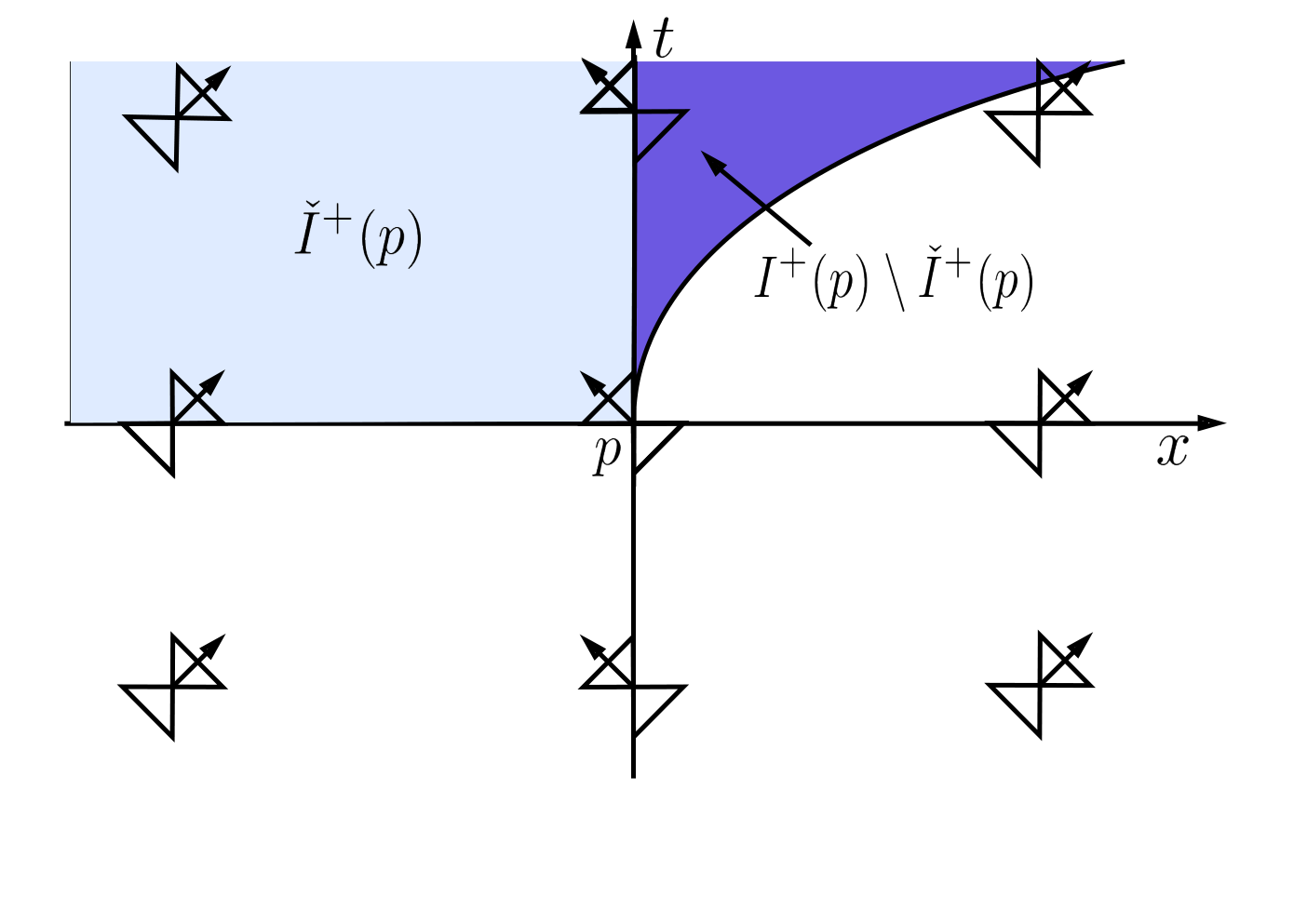
For the point in the figure, the light blue set is the set , while the union of the light blue and dark blue sets (including all points on the -axis above the point ) is the set . As such, non-trivial internal bubbling occurs for this metric. In particular,
- •
- •
Example 3.3.
In [CG12], the metric
| (3.2) |
for with was considered, which exhibits external bubbling. In our next example, we define a different metric where the external bubbling effect is localised. We then glue this metric into Example 3.2 above to construct a metric where there exists a point such that and at the same time.
Let , , and . Let , and fix such that . We define the regions
We consider the Lorentzian metric (3.1) where the function is defined as follows:
-
For , we define
-
For , let
-
We choose the function on the set in such a way that
- (i).
is continuous on ;
- (ii).
For each fixed the angle is a non-decreasing function of , i.e., for each fixed , the function is non-decreasing;
- (iii).
The light cones match up to those on the boundary of the sets and . In particular, we require
and
- (i).
Remark 3.4.
The function may be chosen to be smooth away from the -axis and the points of the set that lie on the -axis. Globally, we then have that has Hölder regularity , with .
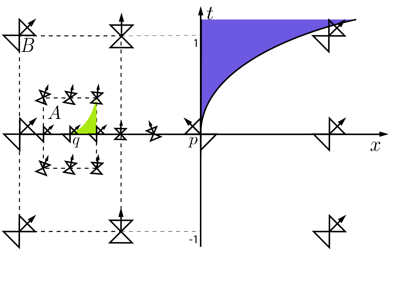
Let be a point in the interior of the set . We denote by the right-moving null generator from that immediately leaves the -axis at , i.e. for all . However, right-moving null generators from can travel along the -axis for a finite time, and then leave the -axis. We denote by the right-moving null generator from that leaves the -axis at the largest value of , i.e. leaves the -axis at the point where . The null generators , later intersect the -axis at the points , , respectively, where . The set contains the area between and up to the -axis, and hence has non-empty interior. As in Example 3.2, for any , the point and contains a subset of the set with non-empty interior. Since is contained in the set , it follows that has non-empty interior as well.
This example therefore answers (5) in the negative, and indeed shows that there exist points in the spacetime such that is non-empty for some cylindrical neighbourhood of , and .
Remark 3.5.
In all of the above examples, the exceptional curves can, in fact, be chosen to be with non-timelike tangent vector at only one point. Heuristically, one might expect that the seemingly innocuous change of allowing curves that have timelike tangent vector except at a finite number of points at which the tangent vector may be null should not affect chronological pasts and futures. However, our examples show that in fact all of the pathologies exhibited above would persist if this definition were adopted.
4. Conclusions
The following diagram collects the (non-)implications between the causal regularity properties we have studied in the previous sections. Let be a continuous spacetime and recall that . Then:
Here, \raisebox{0.4pt}{\tiny$1$}⃝ was shown in [CG12, Cor. 1.17]. Irreversibility of this arrow can be seen by considering a metric that is conformally equivalent to the Minkowski metric via a non-Lipschitz factor. Of more interest is the fact that warped products with one-dimensional base (i.e., metrics of the form with any Riemannian metric and continuous) are causally plain for continuous, not necessarily Lipschitz, warping functions , cf. [AGKS19]. Equivalence \raisebox{0.4pt}{\tiny$2$}⃝ is Corollary 2.16. Irreversibility in \raisebox{0.4pt}{\tiny$3$}⃝, \raisebox{0.4pt}{\tiny$4$}⃝ and \raisebox{0.4pt}{\tiny$8$}⃝, as well as the claims in \raisebox{0.4pt}{\tiny$9$}⃝ follow from [CG12, Ex. 1.12] and Example 3.2, respectively. Equivalence \raisebox{0.4pt}{\tiny$5$}⃝ holds by Theorem 2.15, while \raisebox{0.4pt}{\tiny$6$}⃝ is a consequence of Theorem 2.12. The claims in \raisebox{0.4pt}{\tiny$7$}⃝ follow from [CG12, Ex. 1.12] and Example 3.1. Finally, Example 3.2 entails irreversibility of \raisebox{0.4pt}{\tiny$8$}⃝.
The watershed in this chain of implications is the case of causally plain spacetimes. Indeed, for such metrics all versions of chronological futures and pasts coincide. Moreover, there are no bubble sets, chronological futures and pasts are open and the standard push-up properties hold. Indeed, it was demonstrated in [KS18, Sec. 5.1] that strongly causal and causally plain spacetimes form strongly localisable Lorentzian length spaces, implying that their causality theory is optimal in the sense of synthetic low regularity Lorentzian geometry.
On the other hand, the examples in Section 3 demonstrate that continuous but non-Lipschitz spacetimes display a number of unexpected new causal phenomena that are entirely absent from the causally plain setting. The most drastic of these is the occurrence of non-open chronological futures/pasts. It is no exaggeration to state that openness of is ubiquitous throughout standard causality theory. For example, Theorem 2.10 (iv) is a property that features prominently in proofs of the singularity theorems of General Relativity: for the most general version of the causal part of these theorems we refer to [Min19, Sec. 2.15] (cf., in particular, the proof of Penrose’s singularity theorem [Min19, Thm. 65] that relies on this property in the form of [Min19, Thm. 20]). That this condition is (for chronological spacetimes) in fact equivalent to openness of chronological futures/pasts (Theorem 2.10 (i)) is a strong indication that it is preferable to adopt a different definition for these sets in regularities below Lipschitz. Indeed, the arguments put forward in this paper suggest that the optimal strategy for obtaining a satisfactory causality theory is the following:
- •
In order to derive the maximal benefit from limit curve theorems, set (cf. Lemma 2.9).
- •
To guarantee openness of chronological futures and pasts and to avoid interior bubbling, set . Then in fact by Lemma 2.7.
The first point here is valid across all regularities of the metric. For the second one, we have seen in Theorem 2.15 that for spacetimes without internal bubbling (in particular: for Lipschitz spacetimes) the choice of class of curves makes no difference, while the examples in Section 3 clearly underline the advantage of adhering to this convention for non-Lipschitz metrics.
While this strategy returns us to the “unhandy situation in which timelike and causal paths have completely different properties” [Chr11, p. 14], it appears to us to be the most fitting approach. Moreover, note that, in fact, several fundamental works on low regularity Lorentzian geometry have adopted these conventions, in particular [Min15, Min19, BS18] and, in the timelike case, [GL17, Sbi18a]. On the other hand, in synthetic approaches to low regularity Lorentzian geometry (such as [KS18, GKS19]), where this strategy is not an option (due to the absence of a differentiable structure), phenomena such as the ones laid out in Section 3 have to be taken into consideration.
Acknowledgement
We are indebted to two anonymous referees for several remarks that have led to considerable improvements of the manuscript.
References
- [AB08] S. B. Alexander and R. L. Bishop. Lorentz and semi-Riemannian spaces with Alexandrov curvature bounds. Comm. Anal. Geom., 16(2):251–282, 2008.
- [AGKS19] S. B. Alexander, M. Graf, M. Kunzinger, and C. Sämann. Generalized cones as Lorentzian length spaces: Causality, curvature, and singularity theorems. In preparation. 2019.
- [AT04] L. Ambrosio and P. Tilli. Topics on analysis in metric spaces, volume 25 of Oxford Lecture Series in Mathematics and its Applications. Oxford University Press, Oxford, 2004.
- [BEE96] J. K. Beem, P. E. Ehrlich, and K. L. Easley. Global Lorentzian geometry, volume 202 of Monographs and Textbooks in Pure and Applied Mathematics. Marcel Dekker Inc., New York, second edition, 1996.
- [BS18] P. Bernard and S. Suhr. Lyapounov Functions of Closed Cone Fields: From Conley Theory to Time Functions. Comm. Math. Phys., 359(2):467–498, 2018.
- [Chr91] P. T. Chruściel. On uniqueness in the large of solutions of Einstein’s equations (“strong cosmic censorship”). Proceedings of the Centre for Mathematics and its Applications, Australian National University 27, Canberra 1991.
- [Chr11] P. T. Chruściel. Elements of causality theory. 2011. arXiv:1110.6706 [gr-qc].
- [CG12] P. T. Chruściel and J. D. E. Grant. On Lorentzian causality with continuous metrics. Classical Quantum Gravity, 29(14):145001, 32, 2012.
- [Fat15] A. Fathi. Time functions revisited. Int. J. Geom. Methods Mod. Phys., 12(8):1560027, 12, 2015.
- [FS12] A. Fathi and A. Siconolfi. On smooth time functions. Math. Proc. Cambridge Philos. Soc., 152(2):303–339, 2012.
- [GL17] G. J. Galloway and E. Ling. Some remarks on the -(in)extendibility of spacetimes. Ann. Henri Poincaré, 18(10):3427–3447, 2017.
- [GLS18] G. J. Galloway, E. Ling, and J. Sbierski. Timelike completeness as an obstruction to -extensions. Comm. Math. Phys., 359(3):937–949, 2018.
- [Ger70] R. Geroch. Domain of dependence. J. Mathematical Phys., 11:437–449, 1970.
- [GGKS18] M. Graf, J. D. E. Grant, M. Kunzinger, and R. Steinbauer. The Hawking–Penrose Singularity Theorem for -Lorentzian Metrics. Comm. Math. Phys., 360(3):1009–1042, 2018.
- [GL18] M. Graf and E. Ling. Maximizers in Lipschitz spacetimes are either timelike or null. Classical Quantum Gravity, 35(8):087001, 6, 2018.
- [GKS19] J. D. E. Grant, M. Kunzinger, and C. Sämann. Inextendibility of spacetimes and Lorentzian length spaces. Ann. Glob. Anal. Geom. 55:133-147, 2019.
- [Har82] S. G. Harris. A triangle comparison theorem for Lorentz manifolds. Indiana Univ. Math. J., 31(3):289–308, 1982.
- [HE73] S. W. Hawking and G. F. R. Ellis. The large scale structure of space-time. Cambridge University Press, London-New York, 1973. Cambridge Monographs on Mathematical Physics, No. 1.
- [HW51] P. Hartman and A. Wintner. On the problems of geodesics in the small. Amer. J. Math., 73:132–148, 1951.
- [Kri99] M. Kriele. Spacetime, volume 59 of Lecture Notes in Physics. New Series m: Monographs. Springer-Verlag, Berlin, 1999. Foundations of general relativity and differential geometry.
- [KS18] M. Kunzinger and C. Sämann. Lorentzian length spaces. Ann. Glob. Anal. Geom. 54(3):399–447, 2018.
- [KSS14] M. Kunzinger, R. Steinbauer, and M. Stojković. The exponential map of a -metric. Differential Geom. Appl., 34:14–24, 2014.
- [KSSV14] M. Kunzinger, R. Steinbauer, M. Stojković, and J. A. Vickers. A regularisation approach to causality theory for -Lorentzian metrics. Gen. Relativity Gravitation, 46(8):Art. 1738, 18, 2014.
- [KSSV15] M. Kunzinger, R. Steinbauer, M. Stojković, and J. A. Vickers. Hawking’s singularity theorem for -metrics. Classical Quantum Gravity, 32(7):075012, 19, 2015.
- [KSV15] M. Kunzinger, R. Steinbauer, and J. A. Vickers. The Penrose singularity theorem in regularity . Classical Quantum Gravity, 32(15):155010, 12, 2015.
- [Lec16] A. Lecke. Non-smooth Lorentzian geometry and causality theory. PhD thesis, University of Vienna, Faculty of Mathematics, 2016.
- [Min08] E. Minguzzi. Limit curve theorems in Lorentzian geometry. J. Math. Phys., 49(9):092501, 18, 2008.
- [Min15] E. Minguzzi. Convex neighborhoods for Lipschitz connections and sprays. Monatsh. Math., 177(4):569–625, 2015.
- [Min19] E. Minguzzi. Causality theory for closed cone structures with applications. Reviews in Mathematical Physics, 31(5):1930001, 139, 2019.
- [MS08] E. Minguzzi and M. Sánchez. The causal hierarchy of spacetimes. In Recent developments in pseudo-Riemannian geometry, ESI Lect. Math. Phys., pages 299–358. Eur. Math. Soc., Zürich, 2008.
- [Nat55] I. P. Natanson. Theory of functions of a real variable. Frederick Ungar Publishing Co., New York, 1955. Translated by Leo F. Boron with the collaboration of Edwin Hewitt.
- [O’N83] B. O’Neill. Semi-Riemannian geometry with applications to relativity, volume 103 of Pure and Applied Mathematics. Academic Press, Inc. [Harcourt Brace Jovanovich, Publishers], New York, 1983.
- [Pen72] R. Penrose. Techniques of differential topology in relativity. Society for Industrial and Applied Mathematics, Philadelphia, Pa., 1972. Conference Board of the Mathematical Sciences Regional Conference Series in Applied Mathematics, No. 7.
- [Säm16] C. Sämann. Global hyperbolicity for spacetimes with continuous metrics. Ann. Henri Poincaré, 17(6):1429–1455, 2016.
- [Sbi18a] J. Sbierski. The -inextendibility of the Schwarzschild spacetime and the spacelike diameter in Lorentzian geometry. J. Differential Geom., 108(2):319–378, 2018.
- [Sbi18b] J. Sbierski. On the proof of the -inextendibility of the Schwarzschild spacetime. Journal of Physics: Conference Series, 968(1):012012, 2018.
- [SS18] C. Sämann and R. Steinbauer. On geodesics in low regularity. Journal of Physics: Conference Series, 968(1):012010, 2018.
- [Wal84] R. M. Wald. General relativity. University of Chicago Press, Chicago, IL, 1984.