Plasma Lenses for Relativistic Laser Beams in Laser Wakefield Accelerators

Nowadays petawatt lasers have become high-priority tools for studying the intrinsic properties of the microscopic physical world SEL. Manipulation of such powerful lasers is a big challenge due to the lack of high damage-threshold optical materials. The current solution is to use large beam apertures so that the laser power is spread across a large area of the optical element to prevent damage. For example, $\rm SiO_{2}$ has a damage threshold of the order of $1\text{\,}\mathrm{J}\mathrm{/}\mathrm{c}\mathrm{m}^{2}$ if it is irradiated by a femtosecond laser Gallais et al. 2015. If we assume the laser pulse duration is $50\text{\,}\mathrm{f}\mathrm{s}$, the wavelength is $800\text{\,}\mathrm{n}\mathrm{m}$ and the laser beam is perfectly Gaussian, to focus a $1\text{\,}\mathrm{P}\mathrm{W}$ laser beam a mirror with a $0.34\text{\,}\mathrm{m}$ diameter is required to prevent mirror damage, resulting in high costs for high-quality focusing optics. The cost issue is compounded by the fact that for each laser system multiple focusing systems are required for different applications: short focal length optics for laser-solid interactions and long focal length ones for laser-gas interactions. A particularly demanding application is the laser wakefield accelerator (LWFA), where the laser beam should be focused to a matched spot size that stabilizes laser propagation in the plasma, with the size of this matched spot changing with laser power, the plasma density, and the plasma channel depth in the external guiding case Esarey et al. 2009; Benedetti et al. 2012; Lu et al. 2007; Kostyukov et al. 2004; Poder et al. 2018. For photon-nuclear interaction applications a changeable laser spot size is also advantageous for maximizing the electron flux Zeng and Tesileanu 2017.

In order to avoid damaging laser optics, the beam near field diameter $D$ must scale as $D\propto\sqrt{P}$ with laser power $P$. The f-number $N\equiv f/D\propto kw_{0}$, where $f$ is the focal length, $w_{0}$ is the laser beam waist at focus and $k=2\pi/\lambda$ is the wavenumber for laser with wavelength $\lambda$. Thus $f\propto w_{0}\sqrt{P}\propto P/a_{0}$, where $a_{0}\approx 8.5\times 10^{-10}\lambda\left[{\rm\mu m}\right]\sqrt{I_{0}\left[{\rm W/cm^{2}}\right]}\propto\sqrt{P}/w_{0}$ is the normalized laser amplitude and $I_{0}$ is the peak intensity. For LWFA studies an optimum $a_{0}$ is required even with increasing $P$ Lu et al. 2007, resulting in the focal length $f\propto P$ being extremely long. For example, focal lengths on the order of 10 meters are required for $1\text{\,}\mathrm{P}\mathrm{W}$ lasers Leemans et al. 2014, while for $100\text{\,}\mathrm{P}\mathrm{W}$ lasers the focal lengths would be on the order of 1000 meters. With such scales presenting obvious difficulties, a focusing system with a variable focal spot size and small footprint is urgently required.

In this paper, we introduce such a focusing system employing the laser self-focusing effect in plasmas Max et al. 1974. The scheme is illustrated in Fig. 1. A high power laser beam is pre-focused to $z_{0}$ by a conventional focusing system with a focal length of $f_{0}$ to a spot size of $w_{0}$. After propagating a distance $d$, the laser enters the plasma region starting at $z_{1}$. After another distance $l$, the laser beam is refocused to a spot size $w_{2}$ at $z_{2}$ because of the self-focusing effects Max et al. 1974. Consequently the total function of this system is to focus the laser to a spot size of $w_{2}$ within a distance of $L=f_{0}+d+l$. Due to the strong plasma response, $L$ can be much shorter than a conventional focusing system resulting in the same spot size. In addition, $w_{2}$ is adjustable by changing $d$, $l$ and the plasma density $n_{p}$.

This paper is organized as follows. In Sec. II an analytical model describing the plasma lens is developed. In Sec. III an empirical model is found based on particle-in-cell simulations. The empirical and analytical model are compared in Sec. IV and a full scale LWFA simulation employing the proposed plasma lens is presented in Sec. V.

The evolution of the laser pulse in an underdense plasma in the long pulse and slow profile variation assumptions is given by Mora and Thomas M. Antonsen 1997

where $z$ is the laser propagation distance, $n$ is the local plasma electron density and $\gamma$ is the plasma electron Lorentz factor. Normalized units are adopted with densities being normalized to the background plasma density $n_{p}$, wavenumbers to the plasma wavenumber $k_{p}=\sqrt{4\pi r_{e}n_{p}}$ where $r_{e}\approx 2.82\times 10^{-15}\ \rm m$ is the classical electron radius, and lengths normalized to the plasma skin depth $k_{p}^{-1}$. The cylindrically symmetrical normalized laser vector potential $\tilde{a}$, including the transverse phase modulation but excluding the laser quiver factor $\exp\left(-ikz+i\omega t\right)$, is given by

where $r$ is radius, $a=a\left(z\right)$ is the axial normalized laser vector potential amplitude, $u=u\left(z\right)$ is the spatial phase modulation factor (effectively, the radius of the wavefront curvature is $k/2u$), and $w=w\left(z\right)$ is the laser spot size.

In general, solving Eq. (1) analytically is difficult. However, it has been found that under weakly relativistic assumptions where the plasma density is unperturbed $n=1$, the approximate solution of Eq. (1) for a linearly polarized laser beam can be obtained by calculus of variations Anderson and Bonnedal 1979; Sheng et al. 1996; Sprangle et al. 1987 as the following (derivation is given in App. C):

where Eq. (3) represents the energy conservation law and Eq. (4) describes the evolution of the laser spot size in the weakly relativistic regime $a\lesssim 1$ Tzeng and Mori 1998.

We apply Eq. (4) to our case with the initial conditions at the vacuum-plasma interface ($z=z_{1}$) reading

where $z_{R}=kw_{0}^{2}/2$ is the Rayleigh length. After integrating Eq. (4) the refocused spot size can be found by requiring $\mathrm{d}w/\mathrm{d}z=0$ and is given by

The length of the plasma lens $l$ is given by

with the limit

Thus $d_{\rm M}$ is the upper limit of the pre-focusing distance $d$ for self-refocusing to occur.

Eqs. (7), (8) and (9) show that in the analytical model the effective laser spot size $w_{2}$ and the plasma lens thickness $l$ are the functions of the normalized laser vector potential amplitude at vacuum focus $a_{0}$, the vacuum focal size $w_{0}$, the vacuum Rayleigh length $z_{R}$ and the pre-focusing distance $d$ (all the lengths are normalized to $k_{p}^{-1}$). Effectively, $w_{2}$ and $l$ are functions of $k$ (normalized to $k_{p}$), $w_{0}$, $a_{0}$ and $d$, indicating the parameter space to be scanned in the simulation studies in Sec. III.

The analytic model presented in Sec. II is valid for $a_{0}\lesssim 1$, while for realistic LWFA applications a relativistic laser intensity is required. To examine the behaviour of the plasma lens in the highly relativistic regime, three-dimensional (3D) particle-in-cell (PIC) simulations using the code OSIRIS Fonseca et al. 2002 were performed. To characterize the plasma lens, the refocused spot size $w_{2}$ and plasma lens length $l$ were found by scanning a four-dimensional parameter space of ($k$, $w_{0}$, $a_{0\max}$, $d$), where $a_{0\max}$ is the peak normalized laser amplitude along the laser co-moving coordinate $\xi=z-ct$ (i. e. at the vacuum focus, $a_{0}$ is a function of $\xi$, varies between 0 and $a_{0\max}$). The longitudinal profile of the laser pulse is a bell shape (both the rise and fall envelopes of the laser take the form $10X^{3}-15X^{4}+6X^{5}$ in the range $0\leq X\leq 1$ where $X=\left|\xi-\xi_{0}\right|/\tau$ and $\xi_{0}$ is the pulse center), thus the averaged $a_{0}$ is approximately $a_{0\max}/2$. The initial full-width-at-half-maximum pulse duration was $\tau_{\mathrm{FWHM}}=4$ (time is normalized to $\omega_{p}^{-1}=k_{p}^{-1}c^{-1}$). The simulations were performed using a moving window of length 10, co-moving with the laser pulse towards the positive $z$ direction with the speed of light. The transverse extent of the simulation box was adjusted to be between $10w_{2}$ and $12w_{2}$. In order to ensure convergence, two resolutions for each of the simulations were used as shown in Tab. 1. Simulation time steps were set close to the Courant condition to prevent numerical dispersion. The number of macro-particles per cell is 8 and they are initiated with a thermal momentum of $p_{\rm t}/m_{e}c=0.01$.

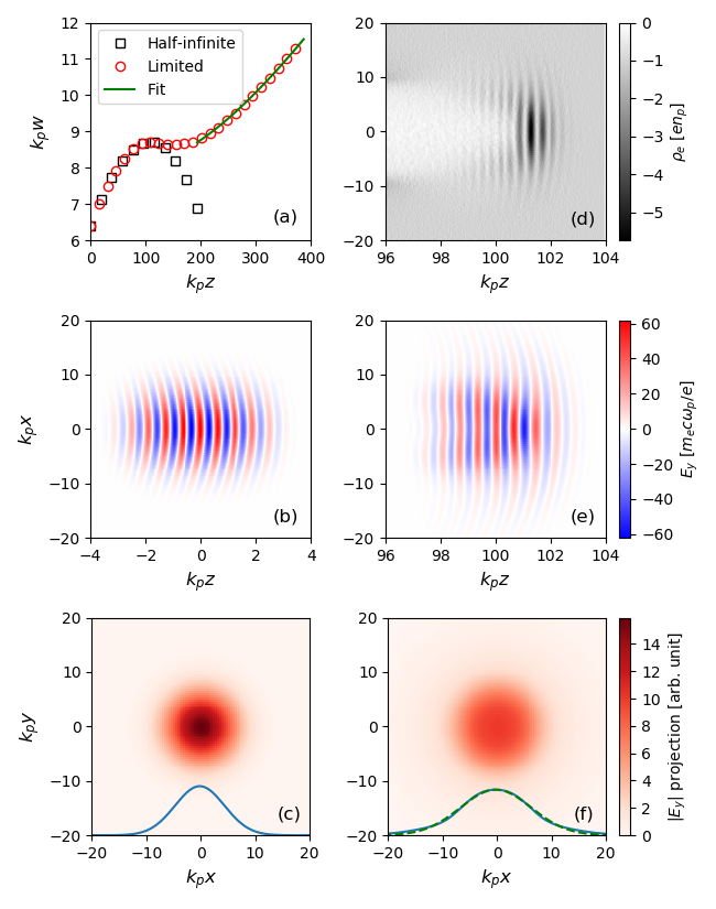
For each simulation, snapshots of the absolute value of the laser electric field are projected to the $x$-$y$ plane (front view). Two-dimensional Gaussian fits are then performed to obtain the spot size $w$ for each snapshot. Example simulation results are shown in Fig. 2. A laser with $k=10$ and $a_{0\max}=10$ is focused to $w_{0}=4$ at $z=-100$. It then enters the plasma region starting at $z=0$ and self-refocusing occurs. As seen in Fig. 2 (a), $w$ reaches a local maximum $w_{2}=8.7$ at $z=z_{2}=104\pm 4$ for the half-infinite plasma case, plotted as black squares. In the case of a limited plasma region ending at $z=z_{2}$ which is plotted as red circles in Fig. 2 (a), after the plasma ends the laser spot size approximately evolves as

where $w_{0e}$ is the effective focal size, $z_{0e}$ is the effective focal position and $z_{Re}=kw_{0e}^{2}/2$ is the effective Rayleigh length with $k=10$ in this case. The evolution of the spot size in the vacuum of the rear side can be fitted by Eq. (10), resulting in $z_{0e}=53.8$ and $w_{0e}=8.0$. The data in the region $z<200$ are ignored in the fit, because the far-distance measurement can better represent the beam size due to the non-perfectly Gaussian profile of the laser beam. The mismatch $z_{0e}\neq z_{2}$ and $w_{0e}\neq w_{2}$ is due to the laser transverse profile not being perfectly Gaussian at $z=z_{2}$, as highlighted in Fig. 2 (e) and (f). However, with only a $10\%$ difference between the spot sizes, $w_{2}$ is used as the effective focal size of our plasma lens in the following.

By comparing Eqs. (7) and (11), an analytical correspondence of $\zeta$ can be written as

This suggests $\zeta_{a}$ is mainly dependent on, but smaller than the Rayleigh length $z_{R}$, which is similar to the empirical expression for $\zeta$ in Eq. (14). Also by comparing Eqs. (8) and (15) an analytical correspondence of $\chi$ can be found as

In the limit of the laser power being much higher than the critical power for self-focusing $a_{0}^{2}w_{0}^{2}/32\gg 1$ Sprangle et al. 1987, applying the weakly relativistic approximation $a_{0}\lesssim 1$ (thus $w_{0}\gg 1$) and with the assumption of short distance from vacuum focus to plasma $d\ll z_{R}$, Eq. (20) reduces to $\chi_{a}\propto w_{0}^{-2}$, which is again similar to the empirical expression for $\chi$ in Eq. (17).

The variation of the refocused spot size $w_{2}$ and the plasma lens thickness $l$ with pre-focusing distance $d$ in both the empirical formulas and the analytical model (by setting $a_{0}=a_{0\max}/2$) is compared to some simulations in Fig. 9. It is evident that in most cases the empirical formulas fit the simulations well, but the analytical model only partially agrees with the simulations for a smaller $a_{0\max}$. The disagreement arises from the fact that for $a_{0\max}\gg 1$, the plasma cannot be regarded as unperturbed and thus the weekly relativistic assumption used in the analytical model is no longer applicable.

In order to show the physical scales of the plasma lens explicitly, unnormalized units will be used in this section. Using Eqs. (11), (14), (18), and applying the matching condition Lu et al. 2007 at $z_{2}$ (i. e. $k_{p}w_{2}=2\sqrt{a_{2}}$), A plasma lens is designed for a $1\text{\,}\mathrm{P}\mathrm{W}$, $800\text{\,}\mathrm{n}\mathrm{m}$ laser with $108\text{\,}\mathrm{f}\mathrm{s}$ pulse duration. A linear density ramp from $z=-20k_{p}^{-1}=$-216\text{\,}\mathrm{\SIUnitSymbolMicro m}$$ to $z=0$ is followed by a density plateau with density $n_{p}=$2.43\text{\times}{10}^{17}\text{\,}{\mathrm{cm}}^{-3}$$ (thus $k_{p}^{-1}=$10.8\text{\,}\mathrm{\SIUnitSymbolMicro m}$$ and $\omega_{p}^{-1}=$35.9\text{\,}\mathrm{f}\mathrm{s}$$). The laser frequency is thus $\omega/\omega_{p}=k/k_{p}=84.7$, the FWHM pulse duration is $\tau=3\omega_{p}^{-1}$ and the laser vacuum focus is set to $z=-80k_{p}^{-1}=$-864\text{\,}\mathrm{\SIUnitSymbolMicro m}$$ with $w_{0}=2k_{p}^{-1}=$21.6\text{\,}\mathrm{\SIUnitSymbolMicro m}$$, thus $a_{0}=8$. The influence of the density transition region is neglected, thus the pre-focusing distance is $k_{p}d=80$. According to Eqs. (11), (14) and (18), this setup results in $w_{2}=4k_{p}^{-1}=$43.2\text{\,}\mathrm{\SIUnitSymbolMicro m}$$ and $a_{2}=4$, with plasma lens thickness $l=397k_{p}^{-1}=$4.29\text{\,}\mathrm{mm}$$.

A confirmation simulation is run with the parameters just discussed, setting the simulation box size to $17k_{p}^{-1}\times 40k_{p}^{-1}\times 40k_{p}^{-1}$ and number of cells to $4096\times 256\times 256$. The time step is $\Delta t=4.147\times 10^{-3}\omega_{p}^{-1}$. Snapshots of a transverse slice through the laser pulse and laser spot size evolution are shown in the top panels of Fig. 10. It is evident that at $z=l=397k_{p}^{-1}$, the laser size $w$ is increased to $4k_{p}^{-1}$ and the bubble radius is also approximately $4k_{p}^{-1}$. At later times the laser front becomes not well guided and at around $z=2000k_{p}^{-1}$ the spot size $w$ stabilizes at about $5.9k_{p}^{-1}$. The source of the mismatch between the local maximum of the spot size $w$ and the prediction from the empirical formulas can be the change of pulse duration; $\omega_{p}\tau=3$ is used here while the value $\omega_{p}\tau=4$ was used for obtaining the empirical formulas. Another source of error can be the extrapolation of the results for $10\leq k/k_{p}\leq 40$ to $k/k_{p}=84.7$. Nevertheless, the bubble radius remains at about $4k_{p}^{-1}$ for later times. Although the plasma lens parameters are chosen to satisfy Eq. (35) to avoid self-injection, a small bunch of electrons with a charge of $16\text{\,}\mathrm{p}\mathrm{C}$ is self-injected due to bubble evolution. However, the charge of this bunch is negligible compared to the loading capacity of this bubble which is a few nanocoulombs according to Eq. (10) of Ref. Lu et al. 2007 and Eq. (10) of Ref. Tzoufras et al. 2008. Moreover, According to Eqs. (3) and (4) of Ref. Lu et al. 2007, both the pump depletion length $l_{\rm dep}\approx\left(k/k_{p}\right)^{2}\omega_{p}\tau k_{p}^{-1}=2.15\times 10^{4}k_{p}^{-1}=$232\text{\,}\mathrm{m}\mathrm{m}$$ and the dephasing length $l_{d}\approx\frac{2}{3}\left(k/k_{p}\right)^{2}w_{2}=1.91\times 10^{4}k_{p}^{-1}=$206\text{\,}\mathrm{m}\mathrm{m}$$ are much larger than $l$, thus the plasma lens does not significantly shorten the acceleration length.

To highlight the performance of the plasma lens, a simulation without the plasma lens was performed with $a_{0}=4$, $w_{0}=4k_{p}^{-1}=$43.2\text{\,}\mathrm{\SIUnitSymbolMicro m}$$ and $k_{p}d=0$. The results of this simulation are shown in the bottom panels in Fig. 10. The spot size evolution, shown in Fig. 10 (d) and Fig. 10 (f) for the simulation with and without the plasma lens, respectively, is evidently not the same for the two cases. Nevertheless, the laser spot size approaches $k_{p}w=5.5$ in the case without the plasma lens, which is similar to the value of $k_{p}w=5.9$ for the simulation with the plasma lens. The spot size does not become stabilized at the matched value 4 is again due to the the front of the laser being not very well guided, thus increasing the front-view spot size of the laser. Moreover, a bunch of electrons is also injected due to the evolution of the driver in this case, with the charge $15\text{\,}\mathrm{p}\mathrm{C}$ being similar to that in the former case.

The similarities in the results of the two cases clearly highlight the usefulness of the plasma lens. For the $1\text{\,}\mathrm{P}\mathrm{W}$ laser simulated, reaching a spot size of $w_{0}=$21.6\text{\,}\mathrm{\SIUnitSymbolMicro m}$$ requires a focal length of about $10\text{\,}\mathrm{m}$. Employing the plasma lens, a $0.86\text{\,}\mathrm{mm}$ pre-focusing distance and a $4.3\text{\,}\mathrm{m}\mathrm{m}$ long plasma lens result in similar bubble sizes as a different focusing optic with $\sim$20\text{\,}\mathrm{m}$$ focal length would.

A set of plasma lens parameters for LWFAs driven by $800\text{\,}\mathrm{n}\mathrm{m}$ wavelength lasers with powers of $10\text{\,}\mathrm{P}\mathrm{W}$ and $100\text{\,}\mathrm{P}\mathrm{W}$, resulting from our empirical expressions and satisfying the matching condition $k_{p}w_{2}=2\sqrt{a_{2}}$ are shown in Tab. 3. Simulations to verify these parameter sets are, however, extremely consuming in computational resources, thus requiring fast algorithms such as the quasi-3D algorithm Davidson et al. 2015.

A plasma lens based on the self-focusing effect was introduced to overcome the experimental limitations for focusing high power lasers to a variety of spot sizes. With a pre-focusing optical system to focus the laser to a waist of $w_{0}$, adjustable effective focal spot sizes $w_{2}>w_{0}$ can be achieved by changing the pre-plasma focusing distance $d$ and the plasma density $n_{p}$. Empirical formulas for $w_{2}$ and the plasma lens thickness $l$ were developed as Eqs. (11), (14) and (18). The focal length of the system can be reduced by the factor of $w_{2}/w_{0}$ if we compare our plasma lens with conventional focusing elements that result in the same laser spot size. Further reductions of the focal length may be achievable by cascading plasma lenses.

The upper limit of the effective focal spot size is determined by the upper limit of the pre-focusing distance $d_{\lim}$. We found the analytical correspondence $d_{\rm M}$ expressed by Eq. (9) presents a good estimation for $d_{\lim}$ especially when $a_{0\max}$ is not large ($a_{0\max}\leq 6$). A more universal expression for $d_{\lim}$ requires further studies.

References

- (1) http://www.sciencemag.org/news/2018/01/physicists-are-planning-build-lasers-so-powerful-they-could-rip-apart-empty-space, doi:10.1126/science.aat0939.
- Gallais et al. (2015) L. Gallais, D.-B. Douti, M. Commandré, G. Batavičiūtė, E. Pupka, M. Ščiuka, L. Smalakys, V. Sirutkaitis, and A. Melninkaitis, J. App. Phys. 117, 223103 (2015), https://doi.org/10.1063/1.4922353 .
- Esarey et al. (2009) E. Esarey, C. B. Schroeder, and W. P. Leemans, Rev. Mod. Phys. 81, 1229 (2009).
- Benedetti et al. (2012) C. Benedetti, C. B. Schroeder, E. Esarey, and W. P. Leemans, Phys. Plasmas 19, 053101 (2012), https://doi.org/10.1063/1.4707393 .
- Lu et al. (2007) W. Lu, M. Tzoufras, C. Joshi, F. S. Tsung, W. B. Mori, J. Vieira, R. A. Fonseca, and L. O. Silva, Phys. Rev. ST Accel. Beams 10, 061301 (2007).
- Kostyukov et al. (2004) I. Kostyukov, A. Pukhov, and S. Kiselev, Phys. Plasmas 11, 5256 (2004), https://doi.org/10.1063/1.1799371 .
- Poder et al. (2018) K. Poder, J. M. Cole, J. C. Wood, N. C. Lopes, S. Alatabi, P. S. Foster, C. Kamperidis, O. Kononenko, C. A. Palmer, D. Rusby, A. Sahai, G. Sarri, D. R. Symes, J. R. Warwick, S. P. D. Mangles, and Z. Najmudin, Plasma Phys. Control. Fusion 60, 014022 (2018).
- Zeng and Tesileanu (2017) M. Zeng and O. Tesileanu, Plasma Sci. Technol. 19, 070502 (2017).
- Leemans et al. (2014) W. Leemans, A. Gonsalves, H.-S. Mao, K. Nakamura, C. Benedetti, C. Schroeder, C. Tóth, J. Daniels, D. Mittelberger, S. Bulanov, et al., Phys. Rev. Lett. 113, 245002 (2014).
- Max et al. (1974) C. E. Max, J. Arons, and A. B. Langdon, Phys. Rev. Lett. 33, 209 (1974).
- Mora and Thomas M. Antonsen (1997) P. Mora and J. Thomas M. Antonsen, Phys. Plasmas 4, 217 (1997), https://doi.org/10.1063/1.872134 .
- Anderson and Bonnedal (1979) D. Anderson and M. Bonnedal, Phys. Fluids 22, 105 (1979), https://aip.scitation.org/doi/pdf/10.1063/1.862445 .
- Sheng et al. (1996) Z.-M. Sheng, Y. Cui, N. Cheng, and Y. Wei, J. Opt. Soc. Am. B 13, 584 (1996).
- Sprangle et al. (1987) P. Sprangle, C.-M. Tang, and E. Esarey, IEEE Trans. Plasma Sci. 15, 145 (1987).
- Tzeng and Mori (1998) K.-C. Tzeng and W. B. Mori, Phys. Rev. Lett. 81, 104 (1998).
- Fonseca et al. (2002) R. A. Fonseca, L. O. Silva, F. S. Tsung, V. K. Decyk, W. Lu, C. Ren, W. B. Mori, S. Deng, S. Lee, T. Katsouleas, and J. C. Adam, in Computational Science — ICCS 2002, edited by P. M. A. Sloot, A. G. Hoekstra, C. J. K. Tan, and J. J. Dongarra (Springer Berlin Heidelberg, Berlin, Heidelberg, 2002) pp. 342–351.
- (17) In this paper, all the errors from the fits are the standard deviations if not explicitly specified.
- Tzoufras et al. (2008) M. Tzoufras, W. Lu, F. S. Tsung, C. Huang, W. B. Mori, T. Katsouleas, J. Vieira, R. A. Fonseca, and L. O. Silva, Phys. Rev. Lett. 101, 145002 (2008).
- Davidson et al. (2015) A. Davidson, A. Tableman, W. An, F. S. Tsung, W. Lu, J. Vieira, R. A. Fonseca, L. O. Silva, and W. B. Mori, Journal of Computational Physics 281, 1063 (2015).
- Sun et al. (1987) G. Sun, E. Ott, Y. C. Lee, and P. Guzdar, Phys. Fluids 30, 526 (1987), https://aip.scitation.org/doi/pdf/10.1063/1.866349 .
- Wang et al. (2012) W.-M. Wang, Z.-M. Sheng, M. Zeng, Y. Liu, Z.-D. Hu, S. Kawata, C.-Y. Zheng, W. B. Mori, L.-M. Chen, Y.-T. Li, and J. Zhang, Appl. Phys. Lett. 101, 184104 (2012), https://doi.org/10.1063/1.4765056 .
- Pukhov and Meyer-ter Vehn (2002) A. Pukhov and J. Meyer-ter Vehn, Appl. Phys. B 74, 355 (2002).
- Schroeder et al. (2005) C. B. Schroeder, E. Esarey, and B. A. Shadwick, Phys. Rev. E 72, 055401 (2005).
- Kalmykov et al. (2011) S. Y. Kalmykov, A. Beck, S. A. Yi, V. N. Khudik, M. C. Downer, E. Lefebvre, B. A. Shadwick, and D. P. Umstadter, Phys. Plasmas 18, 056704 (2011), https://doi.org/10.1063/1.3566062 .
- Corde et al. (2013) S. Corde, C. Thaury, A. Lifschitz, G. Lambert, K. T. Phuoc, X. Davoine, R. Lehe, D. Douillet, A. Rousse, and V. Malka, Nat. Comm. 4, 1501 (2013).
- Chen et al. (2006) M. Chen, Z.-M. Sheng, Y.-Y. Ma, and J. Zhang, J. Appl. Phys. 99, 056109 (2006), https://doi.org/10.1063/1.2179194 .
- Oz et al. (2007) E. Oz, S. Deng, T. Katsouleas, P. Muggli, C. D. Barnes, I. Blumenfeld, F. J. Decker, P. Emma, M. J. Hogan, R. Ischebeck, R. H. Iverson, N. Kirby, P. Krejcik, C. O’Connell, R. H. Siemann, D. Walz, D. Auerbach, C. E. Clayton, C. Huang, D. K. Johnson, C. Joshi, W. Lu, K. A. Marsh, W. B. Mori, and M. Zhou, Phys. Rev. Lett. 98, 084801 (2007).
- Pak et al. (2010) A. Pak, K. A. Marsh, S. F. Martins, W. Lu, W. B. Mori, and C. Joshi, Phys. Rev. Lett. 104, 025003 (2010).
- McGuffey et al. (2010) C. McGuffey, A. G. R. Thomas, W. Schumaker, T. Matsuoka, V. Chvykov, F. J. Dollar, G. Kalintchenko, V. Yanovsky, A. Maksimchuk, K. Krushelnick, V. Y. Bychenkov, I. V. Glazyrin, and A. V. Karpeev, Phys. Rev. Lett. 104, 025004 (2010).
- Liu et al. (2011) J. S. Liu, C. Q. Xia, W. T. Wang, H. Y. Lu, C. Wang, A. H. Deng, W. T. Li, H. Zhang, X. Y. Liang, Y. X. Leng, X. M. Lu, C. Wang, J. Z. Wang, K. Nakajima, R. X. Li, and Z. Z. Xu, Phys. Rev. Lett. 107, 035001 (2011).
- Pollock et al. (2011) B. B. Pollock, C. E. Clayton, J. E. Ralph, F. Albert, A. Davidson, L. Divol, C. Filip, S. H. Glenzer, K. Herpoldt, W. Lu, K. A. Marsh, J. Meinecke, W. B. Mori, A. Pak, T. C. Rensink, J. S. Ross, J. Shaw, G. R. Tynan, C. Joshi, and D. H. Froula, Phys. Rev. Lett. 107, 045001 (2011).
- Chen et al. (2012) M. Chen, E. Esarey, C. B. Schroeder, C. G. R. Geddes, and W. P. Leemans, Phys. Plasmas 19, 033101 (2012), https://doi.org/10.1063/1.3689922 .
- Zeng et al. (2014) M. Zeng, M. Chen, Z.-M. Sheng, W. B. Mori, and J. Zhang, Phys. Plasmas 21, 030701 (2014), https://doi.org/10.1063/1.4868404 .
- Suk et al. (2001) H. Suk, N. Barov, J. B. Rosenzweig, and E. Esarey, Phys. Rev. Lett. 86, 1011 (2001).
- Geddes et al. (2008) C. G. R. Geddes, K. Nakamura, G. R. Plateau, C. Toth, E. Cormier-Michel, E. Esarey, C. B. Schroeder, J. R. Cary, and W. P. Leemans, Phys. Rev. Lett. 100, 215004 (2008).
- Martinez de la Ossa et al. (2017) A. Martinez de la Ossa, Z. Hu, M. J. V. Streeter, T. J. Mehrling, O. Kononenko, B. Sheeran, and J. Osterhoff, Phys. Rev. Accel. Beams 20, 091301 (2017).
- Umstadter et al. (1996) D. Umstadter, J. K. Kim, and E. Dodd, Phys. Rev. Lett. 76, 2073 (1996).
- Rechatin et al. (2009) C. Rechatin, J. Faure, A. Ben-Ismail, J. Lim, R. Fitour, A. Specka, H. Videau, A. Tafzi, F. Burgy, and V. Malka, Phys. Rev. Lett. 102, 164801 (2009).
- Lehe et al. (2013) R. Lehe, A. F. Lifschitz, X. Davoine, C. Thaury, and V. Malka, Phys. Rev. Lett. 111, 085005 (2013).
- Benedetti et al. (2013) C. Benedetti, C. B. Schroeder, E. Esarey, F. Rossi, and W. P. Leemans, Phys. Plasmas 20, 103108 (2013), https://doi.org/10.1063/1.4824811 .