Independence-Checking Coding for OFDM Channel Training Authentication: Protocol Design, Security, Stability, and Tradeoff Analysis
Abstract
In wireless OFDM communications systems, pilot tones, due to their publicly-known and deterministic characteristic, suffer significant jamming/nulling/spoofing risks. Thus, the convectional channel training protocol using pilot tones could be attacked and paralysed, which raises the issue of anti-attack channel training authentication (CTA), that is, verifying the claims of identities of pilot tones and channel estimation samples. In this paper, we consider one-ring scattering scenarios with large-scale uniform linear arrays (ULA) and develop an independence-checking coding (ICC) theory to build a secure and stable CTA protocol, namely ICC based CTA (ICC-CTA) protocol. In this protocol, pilot tones are not merely randomized and inserted into subcarriers, but also encoded as diversified subcarrier activation patterns (SAPs) simultaneously. Those encoded SAPs, though camouflaged by malicious signals, can be identified and decoded into original pilots, and hence for high-accuracy channel impulse response (CIR) estimation. The CTA security is first characterised by the error probability of identifying legitimate CIR estimation samples. We prove that the identification error probability (IEP) is equal to zero under the continuously-distributed mean angle of arrival (AoA) and also derive a closed-form expression of IEP under the discretely-distributed case. The CTA instability is formulated as the function of probability of stably estimating CIR against all available diversified SAPs. A realistic tradeoff between the CTA security and instability under the discretely-distributed AoA is identified and an optimally-stable tradeoff problem is formulated, with the objective of optimizing the code rate to maximize security while maintaining maximum stability for ever. Solving this, we derive the closed-form expression of optimal code rate. Numerical results finally validate the resilience of proposed ICC-CTA protocol.
Index Terms:
Physical-layer authentication, anti-attack, OFDM, channel training, independence-checking coding.I Introduction
With the evolution of air interface towards 5G, security paradigms for the protection of air interface technologies have attracted increasing attentions in wireless communications systems. Safeguarding the current standard, for instance, orthogonal frequency-division multiplexing (OFDM) or securely implementing the initiation, such as massive antenna technique, gradually come up on the agenda [1]. The common problem encountered is that the imperishable characteristic of wireless channels, such as the open and shared nature, has always been rendering those technologies vulnerable to the growing denial of service (DoS) attacks [2]. A phenomenon, if we notice, has emerged in the physical (PHY) layer that DoS attacks, with moderate size of the involved network segment and modest implementation complexity, have become increasingly common and potent [3]. As their major hacking behaviors, radio jamming (RJ) attacks have been exhibiting its astonishing destructive power on those existing [4] and emerging air interface techniques [5].
Among these RJ attacks, protocol-aware attack serves as the most effective one as the attacker could sense the specific protocols and intensify its effectiveness significantly by jamming a physical layer mechanism instead of data payload directly [6]. The typical case which frequently occurs in massive-antenna OFDM systems is that protocol-aware attackers always show a great appetite for the channel training protocol. In this protocol, frequency-domain subcarrier (FS) channels and channel impulse response (CIR) samples, are estimated to further the high-quality user experience using those estimations. The motivations for this case are twofold. On one hand, multi-antenna OFDM technique has been deployed universally in current commercial and military applications, which incurs huge interests of malicious nodes. Since the channel training protocol requires that deterministic and publicly-known pilot tones should be shared on the time-frequency resource grid (TFRG) by all parties [7], a pilot-aware attacker could sense and acquire the public pilot information, and practically behave in such a way that the regular channel training process may not be maintained as usual [8, 9, 10]. On the other hand, everyone has witnessed the introduction of massive antennas into OFDM technique which has been promoted significantly in the recent practice, such as in 3GPP new radio (NR) specifications. In this era, the precise channel training becomes very crucial to maintaining the significant multiplexing gains of target users. The bad news is that imprecise estimation samples could not only lower down those gains but also benefit others, such as the attacker, due to the high resolution of antenna arrays. What’s more, when the channel training is misguided in favour of attacker, actually without too much efforts, massive antenna arrays in OFDM systems will be well loved by the attacker.
In this context, authenticating channel training becomes very critical to the massive antenna OFDM systems since it determines the authenticity of channel estimation results. Generally, channel training launched by any certain subscriber is authenticated by default through the designated public pilot tones allocated to that subscriber [11, 12]. Applying the same pilot tones as the subscriber at the receiver to channel estimation means the exact authentication for channel training. This process is called the channel training authentication (CTA) which belongs to the field of physical-layer authentication [13]. Intrinsically, exact CTA mainly depends on the authenticity of pilot tones in a sense that the claims of identities of pilot tones should be verified. The uniqueness and non-reproducibility of pilot tones are two foremost requirements which however will no longer hold true when a pilot-aware attacker jams/nulls/spoofs those pilot tones. In practice, attacking CTA process in OFDM systems is a common phenomenon, e.g., in scenarios with tactical consideration [14] or in Long Term Evolution (LTE)-based public safety networks [15]. Those attacks, including pilot tone jamming (PTJ) attack [8], pilot tone nulling (PTN) attack [9] and pilot tone spoofing (PTS) attack [10], are very hard to eliminate once they have occurred successfully.
I-A Related Works
Much of the work related to securing CTA has been investigated thus far. How to detect the alteration to authenticity and how to protect and further maintain the high authenticity are two major branches in this area.
The first attempt for narrow-band single-carrier systems is made in [16] in which the pilot contamination (PC) attack, one type of PTS attack, was introduced and evaluated. Following [16], much of the work was studied, but limited to the detection of authenticity of pilot signals by exploiting the physical layer information, such as auxiliary training or data sequences [17, 19, 18] and some prior-known channel information [20, 21]. Different from those, authors in [22] first studied the advantage of spatial correlation in the maintenance of authenticity of pilots, and found that the natural spatial separation of massive antenna arrays can force PC attack to occur effectively only in a particular angular domain. However, we should never forget that the attacker is out of control. In this regard, PC attack actually becomes more well-directed, rather than less effective.
The first attempt for multi-subcarrier scenarios was presented by Clancy et al. [23], verifying the possibility and effectiveness of PTJ attack. Following this, PTJ attack was then studied for single-input single-output (SISO)-OFDM communications in [8] which also introduced the PTN attack and then extended it to the multiple-input multiple-output (MIMO)-OFDM system [9]. The initial attempt to resolve pilot aware attack for conventional OFDM systems was proposed in [24], that is, transforming the PTN and PTS attack into PTJ attack by randomizing the locations and values of regular pilot tones on time-frequency resource grid (TFRG). It figured out the importance that pilot tone scheduling, even being random, would also affect channel acquisition. Hinted by this, authors in [10] proposed a FS channel estimation framework under the PTS attack by exploiting pilot randomization and the independence component analysis (ICA) theory. One key problem is that the practical subcarriers are not mutually independent in the scenarios with limited channel taps, and thus ICA does not apply in this case. Most importantly, the CIR estimation is impossible. Basically, CIR is very critical to the CTA in future 5G mobile eco-systems in which measuring the multipath before designing systems is mandatory since the channel has to carry the big amount of data for our “everything wireless” applications. The knowledge of the channel response represents the aggregate values of gross physical multipath information. CIR is such a wideband channel characterization and contains all information necessary to simulate or analyze any type of radio transmission through the channel. For instance, the amplitude of channel taps could reflect the sparsity of channel in some cases and their variations could tell us the Doppler spread, coherence bandwidth, and so forth [25].
To solve those issues, our previous work in [26] proposed an independence-checking coding (ICC) method which provides high authenticity guarantee on the FS channel and CIR estimation based on randomized pilot tones. Nevertheless, the influence of randomization on CIR estimation was not evaluated and optimized, which incurs the instability of CIR estimation. In this sense, CTA not only merely requires the high security against attacks, but also strongly and necessarily calls for the high stability of CIR estimation accuracy. As far as we know, there were very few studies jointly considering the security and instability during the channel training phase.

I-B Motivations and Contributions
The hints from the above investigation further motive us to build up a secure CTA protocol for massive-antenna OFDM systems with considerations of the heterogeneity of attack modes and the instability of CIR estimation
Recall that pilot randomization serves as a commonsense technique for defending against pilot-aware attack. However, inserting randomized pilot tones on TFRG solely functions to transform the attack modes such that the attack issue will not be insolvable, rather than to resolve the issue practically. To be more specific, this brings two bottlenecks, i.e., 1) Unpredictable attack modes;
Problem 1 (Attack Model).
A pilot-aware attacker chooses on TFRG a hybrid attack mode including PTJ attack and silence cheating (SC) mode. In PTJ attack mode, two behaviors are available, i. e., wide-band pilot jamming (WB-PJ) attack [27] and partial-band pilot jamming (PB-PJ) attack [28]. In SC mode, the attacker keeps silent for cheating the legitimate node. The legitimate node can never acquire the behaviors of the attacker in advance. All of the three modes can be very effective due to the node transparency (i.e., no association or independent with each other) and should never be ignored.
2) Irreversible pilot information. Randomized pilot information become irreversible in the following sense:
Problem 2.
Randomized pilot information are naturally camouflaged by random channel information. Those information, if transmitted by pilot tones for uplink channel training through wireless channels, cannot be separated and identified.
This problem inspires us to perform the protocol design for the overall channel training process. The guideline for this is presented in Fig. 1 where two key requirements are detailed as follows:
- 1.
Share pilot information through encoded subcarrier activation patterns (SAPs): Selectively activate and deactivate OFDM subcarriers by transmitting pilots on subcarriers or not, and create various SAP candidates. Encode all SAPs as a binary code. Optimize the code set in such a way that arbitrary one SAP, namely, codeword, if suffering a hybrid attack in the wireless environment, are enabled to be separated and identified securely. With this preparation, pilot information is conveyed and encoded as one codeword and further expressed as a SAP. Secure pilot sharing is thus constructed between transceiver pairs.
- 2.
Reuse subcarriers in activation to estimate channels: Generate channel estimators according to the identified pilots and apply them on the activated subcarriers for FS channel estimation. Enhance the pilot identification using the estimated FS channels. Derive CIR estimation samples from the estimated FS channels.
In this methodology, channel estimation coexists with the information coding and the two techniques influence each other. In spite of the security guarantee provided by encoded SAPs, SAP diversification also incurs the uncertainties as to the amount and distribution of subcarriers in activation, further instabilizing the CIR estimation extremely. This entanglement between security and instability motivates us to perform the protocol optimization. The main contributions of this paper are summarized as follows:
- 1.
Protocol Design: First, we establish a fundamental principle for encoding arbitrary SAPs as a binary code set precisely. Following this, we develop an ICC theory to further optimize the code such that arbitrary two codewords in the code, if being superimposed on each other, can be separated and identified securely. In order to evaluate the security for this, we formulate two key performance indicators (KPIs), i.e., the separation error probability (SEP) and identification error probability (IEP). We prove that SEP is always guaranteed to be zero and also derive the analytical expression of IEP. We build up an uplink ICC based CTA (ICC-CTA) protocol in which legitimate transceiver pair encodes and decodes randomized pilot phases securely through the ICC codebook, and then performs FS channel and CIR estimation using the identified pilots.
- 2.
Next, we discover a hidden phenomenon that when FS channel estimation is performed on the basis of this protocol, the array spatial correlation existing in the overlapping subcarriers that also carry information from both the legitimate node and the attacker can further help reduce IEP in one-ring scattering scenarios. At this point, the attacker can actually help the legitimate node to enhance the security. Interestingly, it can be proved that zero IEP cannot be achieved only when the attacker is located in the clusters with the same mean angle of arrival (AoA) as the legitimate node. This principle, in this sense, could facilitate the acquisition of the position of attacker. Theoretically when we consider the mean AoA with continuous probability distribution, the security, in theory, can be perfectly guaranteed. Practically in discretely-distributed case, we give an analytical expression of how much the security could be further improved.
- 3.
Protocol Optimization: Finally, we identify the phenomenon of instable CIR estimation in this protocol and define the stability by the function of probability of stable CIR estimation against diversified SAPs. In the realistic scenario with discretely-distributed mean AoAs, we identify and model the tradeoff between the security and instability. Interestingly, we prove that there always exists an optimally-stable tradeoff for which the CIR estimation can always achieve its optimal stability without losing estimation precision asymptotically. Maintaining this stability, we further determine a closed-form expression of optimal code rate that maximizes the security. This code rate indicates how to flexibly configure the number of activated subcarriers under this hybrid attack such that desirable security and maximum stability of CIR estimation can be both guaranteed.
Organization: In Section II , we present an overview of pilot-aware attack on massive-antenna OFDM systems. In Section III, we introduce an ICC-CTA protocol. FS channel estimation and security enhancement are described in Section IV. Security-instability tradeoff in CIR estimation is provided in Section V. Numerical results are presented in Section VI and finally we conclude our work in Section VII.
Notations: We use boldface capital letters for matrices, boldface small letters for vectors , and small letters for scalars. , , and respectively denotes the conjugate operation, the transpose, the conjugate transpose and the first columns of matrix . denotes the Euclidean norm of a vector or a matrix. is the cardinality of a set. is the expectation operator. denotes the Kronecker product operator. stands for the diagonal matrix with the elements of column vector on its diagonal.
II Overview of Pilot-Aware Attack on Massive-Antenna OFDM Systems
We in this section outline a fundamental overview of CTA issue under pilot aware attack, from a mathematical point of view. This refers to the basic system model, signal model, and channel estimation model. Finally, the pilot randomization technique is described and most importantly, we identify its potential challenges in resolving the attack.

II-A System Description
| Notations | Description |
| ; | Number of antennas at BS; Antenna spacing |
| ; | Angle spread at BS; Mean AoA of Bob, and Ava, |
| ; ; | Total available number of subcarriers within each OFDM symbol time; Length of FFT points |
| Number of subcarriers allocated for Bob and Ava | |
| Index set of total available subcarriers | |
| , | Index set of subcarriers allocated for Bob and Ava |
| ; | Pilot tones for Bob and Ava at the -th subcarrier and -th symbol time |
| , ; , | Uplink training power for Bob and Ava; Pilot phases of Bob and Ava |
| ; | Number of sampled multi-path taps in baseband, Average noise power of BS |
| ; | CIR vectors, respectively from Bob and Ava to the -th receive antenna of Alice |
| ; ; ; | DFT matrix; ; -row matrix of ; -row matrix of . |
| , | AWGN vector at the -th antenna of BS within the -th symbol time |
| , | AWGN vector across subcarriers for -th antenna of BS within -th symbol |
| ; | PDP of the -th path of Bob and Ava |
| Received signal vector at the -th subcarrier and -th OFDM symbol. | |
| ; | ; denotes the quantization resolution |
| , | Index set of ambiguous subcarriers under hybrid attack |
| , | Index set of overlapping subcarriers under hybrid attack |
| , , | Index set of the intersection of with |
| ; | Channel covariance matrix of Bob () and Ava (); |
| ; | Rank of ; Rank of |
| ; | Total number of non-zero digits in S.1 and zero digits in S.2 |
| ; , | Total number of nonzero digits for ; Total number of zero digits for |
| Digit indicated by RS |
We consider a synchronous large-scale multiple-input single-output (MISO)-OFDM system with a -antenna base station (named as Alice) and a single-antenna legitimate user (named as Bob). As shown in Fig. 2, the based station (BS) is equipped with a -spacing directive uniform linear array (ULA) and placed at the origin along the -axis to serve a 120-degree sector that is centered around the -axis (). We assume no energy is received for angles . The summary of notations is given in Table I.
For a typical cellular configuration, the channel from Bob to Alice is a correlated random vector with covariance matrix that depends on the scattering geometry. Assuming a macro-cellular tower-mounted BS with no significant local scattering, the propagation between Bob and Alice is characterized by the local scattering around Bob, resulting in the well-known one-ring model [22]. For OFDM systems with frequency-selective channels, the wide-band configuration is more realistic. Here, we consider the wide-band one-ring scattering model in which Bob is surrounded by local scatterers within [22, 29].This will contribute to the following mathematical characterisation of the advantage of spatial correlation in security provision as an explicit result, rather than a complex and unintuitive implication.
We consider pilot tone based uplink channel training process on time-frequency domain with available subcarriers at each OFDM symbol time. In principle, subcarriers indexed by are employed for pilot tone insertion and the following channel estimation. Those pilot tones, known as reference signals in LTE-A and/or beyond, are deterministic and publicly-known in TFRG. Each transceiver, by sharing those tones, can deduce the FS channels and further estimate the CIR samples. Therefore a single-antenna malicious node (named as Ava) could disturb this training process by jamming/spoofing/nulling those pilot tones. We denote the set of victim subcarriers by and make the following assumption:
Assumption 1.
Ava is surrounded by local scatterers within and always has common or overlapping AoA intervals with Bob, this is,
This assumption is supported by the scenario where a common large scattering body (e.g., a large building) could create a set of angles common to all nodes in the system. In this case, the angular spread of BS is broad and the overlapping of AoA intervals is inevitable. The result is that the channel covariance eigenspaces of Bob and Eva are coupled and the attack is hard to eliminate through angular separation [22].
Assumption 2.
II-B Receiving Signal Model
In this subsection, we introduce the receiving signal model at Alice. To begin with, we will give the concept of pilot insertion pattern (PIP) which indicates the way of inserting pilot tones across subcarriers and OFDM symbols.
Assumption 3 (Frequency-domain PIP).
We in this paper assume , for low overhead consideration and theoretical analysis. Alternatively, we can superimpose onto a dedicated pilot sequence optimized under a non-security oriented scenario and utilize this new pilot for training. At this point, can be an additional phase difference for security consideration. We do not impose the phase constraint on the PIP strategies of Ava, that is, .
Let us proceed to the basic OFDM procedure. First, the frequency-domain pilot signals of Bob and Ava over subcarriers are respectively stacked as by vectors and . Here there exist:
| (1) |
Assume that the length of cyclic prefix is larger than . The parallel streams, i.e., and , are modulated with inverse fast Fourier transform (IFFT). After removing the cyclic prefix at the -th receive antenna and -th OFDM symbol time, Alice derive the time-domain by vector as:
| (2) |
where and are circulant matrices for which the first column of and are respectively given by and . Here, is assumed to be independent with . Taking fast Fourier transform (FFT), Alice finally derives the frequency-domain by signal vector at the -th receive antenna and -th OFDM symbol time as
| (3) |
Throughout this paper, we assume that the CIRs belonging to different paths at each antenna exhibit spatially uncorrelated Rayleigh fading. Without loss of generality, each path has the uniform and normalized power delay profile (PDP) satisfying [31]. For each path, CIRs of different antennas are spatially correlated. With the one-ring scattering model, the correlation between channel coefficients of antennas , is defined by [22, 29]:
| (4) |
Here, are symmetric positive semi-definite matrices. Note that is unknown for Alice and Bob while is known by Alice.
II-C Channel Estimation Model
For the PTS attack, Ava could learn the pilot tones employed by Bob in advance and impersonate Bob by utilizing the same pilot tone learned. There exists and . Signals in Eq. (3) can be rewritten as:
| (5) |
Finally, a least square (LS) based channel estimation is formulated by the equation where is the Moore-Penrose pseudoinverse of . We see that the estimation of is contaminated by with a noise bias when a PTS attack happens. As to the characterisation of PTN attack and PTJ attack, we can refer to the mathematical interpretation in [26].
II-D Influence of Pilot Randomization on Pilot-Aware Attack
Pilot randomization can avoid the pilot aware attack without imposing any prior information on the pilot design. The common method is to randomly select phase candidates. Each of the phase candidates is mapped by default into a unique quantized sample, chosen from the set . Since phase information only provides the security guarantee as shown in Assumption 3, thus without the need of huge overheads, we make the following assumptions:
Assumption 4 (Time-domain PIP).
During two adjacent OFDM symbol time, such as, , two pilot phases and are kept with fixed phase difference, that is, , for reducing the authentication overheads. Here, and are both random but are deterministic and publicly known.
Institutively, how the value increases affects the performance of anti-attack technique. This technique also brings up the subject of Problem 2.
III ICC-CTA Protocol
As shown in the Fig. 1, this section presents the principles of pilot conveying, separation and identification.
III-A Pilot Conveying on Code-Frequency Domain
Basically, the more phases supported in , the higher coding diversity is required, and thus the more available SAPs should be created. Theoretically, this requires a delicately-designed binary code and practically depends on how to activate and deactivate subcarriers as the code indicates. This operation will inevitably induce a concurrence of activated and deactivated subcarriers, and therefore detecting the number of signals coexisting on one subcarrier is a necessary work before coding.
To achieve this goal, we will employ the technique of eigenvalue ratio based detection (ERD) proposed in [32]. Here we consider three symbol time and a receiving signal matrix, denoted by , is created for detection. Given the normalized covariance matrix defined by , we define its ordered eigenvalues by and construct the test statistics by where denotes the decision threshold. The hypothesis means that there exist signals and means the opposite.
III-A1 Construction of Code Frequency Domain
Given the threshold , the cumulative distribution function (CDF) of , denoted by , can be expressed by where [32] . Here denotes CDF of a standard Gaussian random variable. In order to measure how many antennas are required on each subcarrier to achieve a certain , a decision threshold function is derived, with where , . Here , and . The related parameters can be shown as follows:
| (6) |
where there exists
| (7) |
where .
| (8) |
where and we have . For the parameters therein, there exist , , , and . is the Signum function and is the upper incomplete Gamma function.

Using the expression of , we establish a single-subcarrier encoding (SSE) principle to encode the number of detected signals into binary digits, i.e, 0 or 1.
Definition 1 (SSE Principle).
One subcarrier can be precisely encoded if, for any , there exists a positive number such that, for all , is smaller than .
Based on the Definition 1, we can encode the -th subcarrier as a binary digit according to . We should note that is a monotone decreasing function of two independent variables, i.e., and . For a given probability constraint , we could always expect a lower bound such that is satisfied. Under this equation, we could flexibly configure and to make approach zero [32]. We also find that the value of achieving zero- is decreased with the increase of .
To verify this, we consider three OFDM symbols and flexible configuration of , such as, from to . We simulate against various in Fig. 3. As we can see, the required decision threshold is decreased with the increase of the number of antennas. This fact also further verifies the feasibility of Definition 1. For example, we can find a desirable point at where is equal to zero, thus facilitating perfect binary coding for each kind of SAPs.

Based on the formulated binary digits for subcarriers in detection, we denote a set of binary code vectors by with where denotes the maximum length of the code. Then, a code frequency domain could be constructed as a set of pairs with and where is an integer representing the subcarrier index of appearance of the code. This is shown in Fig. 4.
III-A2 Binary Codebook Matrix
On the formulated code-frequency domain, we group the binary digits and construct the binary code by presenting a binary codebook as follows:
Definition 2.
Given a binary matrix with each element satisfying , we denote the -th column of by with . We call a binary codebook matrix and a codeword of of length .
The codebook size is equal to the quantization resolution of phases in the set . Based on this codebook matrix, a mapping from pilot phases, to codewords and further to SAPs is developed in Fig. 4 for pilot conveying.
Pilot conveying provides the basis for pilot separation and identification which also means the codeword separation and identification. Therefore, the performance of CTA becomes totally dependent on the property of binary codebook.
III-B Pilot Separation and Identification Via ICC
In this subsection, we present the ICC theory to optimize the previous binary codebook. Its crucial feature is to create the “difference” by checking the independence of channels experienced by different parties. In what follows, we will introduce the ICC theory by formulating its encoding/decoding principle.
III-B1 Encoding Principle

Based on the Definition 2, we further have the following definition:
Definition 3.
A binary matrix is called a ICC- code of length and order , if for any column set such that , there exist at least a set of rows such that .
For this principle, any two codewords in must superimpose with each other on at least non-zero digits.
Remark 1.
Basically, denotes the discriminatory feature we have created. This feature intrinsically can be seen as a characteristic that there always exist more nonzero digits than zero digits. Returning to the subcarriers, means the available number of overlapping subcarriers for channel estimation. The overlapping of subcarriers means the coexistence of signals from two nodes on the same subcarrier and same OFDM symbol time.
Theorem 1.
The weight of ICC- code of length and order satisfies with . is an integer smaller than .
Proof.
See proof in Appendix VIII-A ∎
Here and in the following sections, we assume the ratio of two integer is always kept to be an integer without loss of generality. Based on the theorem, we can derive the number of codewords or namely the columns in , by a binomial coefficient . Then we have the following proposition about the code rate:

Proposition 1.
The code rate of ICC- code, defined by , is calculated as:
| (9) |
III-B2 Decoding Procedure
Despite the fact that the encoding principle provides the discriminatory feature of ICC, Alice has to construct a decoding principle according with this feature to perform codeword separation and identification
Considering the hybrid attack environment, Alice could recognize three types of results on the -th subcarrier : Case 1:None of Bob and Ava transmits signals. Case 2: Bob and Ava both transmit signals. Case 3: One unknown node (Bob or Ava) transmits signals. Obviously, Alice can identify the behaviors in the first two cases but this cannot work well in Case 3 due to the ambiguity of superposition operation of signals on subcarriers. For simplicity, we define the subcarriers in Case 1 and Case 2 as the deterministic subcarriers while those in Case 3 are defined as the ambiguous subcarriers. The related decoding principle is depicted in Fig. 5.
Now that we have explored the principle of ICC method in theory, we ought to look at its performance evaluation.
Proposition 2.
SEP, defined by error probability of separating two right codewords from the observed codeword, is zero.
It is sufficiently feasible that the distance between Bob and Ava can guarantee that their channels fade independently with each other. The inner product of high-dimensional receiving signals on different subcarriers is therefore always precisely measured under massive antennas, providing the perfect differential decoding and thus perfect pilot separation in Fig. 5.
Theorem 2.
IEP, defined by the error probability of identifying Bob’s codeword from the two separated codewords, is given by
| (10) |
Proof.
See proof in Appendix VIII-B. ∎
The overall pilot conveying, separation and identification can be seen in part of Fig. 6.
IV FS Channel Estimation and Security Enhancement
In this section, we continue our design work for the ICC-CTA protocol architecture and focus on the FS channel estimation. Two questions will be answered further:
Question 1.
How to estimate FS channels based on the identified pilots?
Question 2.
Is it possible to improve the security performance of ICC theory by further digging the properties of estimated FS channels ?
IV-A FS Channel Estimation
It is well-known that LS estimator is a natural choice when there is no attack. In this subsection, we only consider the FS channel estimation under PTJ attack shown in the attack model in Introduction part.
In principle, performing linear channel estimation requires specifying the receiving signal model and linear decorrelating estimator (LDE) that weights on the receiving signals for channel estimation.
Let us consider the construction of LDE. Basically, Alice examines the decoded pilots which can be, 1) successfully identified; ( no identification error) or 2) confusing (identification error happens). We in this section consider the latter and forget the case without identification error. In this way, the estimator to be designed naturally apply to the case without identification error. Within two OFDM symbol time, i.e., and , Alice could collect two confusing pilot vectors defined by and where and . The notation of can be found in Assumption 3. Here the confusing case happens when Ava keeps the same frequency-domain and time-domain PIP as Bob, which is proved in Remark 2. Then we use the notation of with the only difference, that is, different value with .
Then we consider the receiving signal model for which two facts involved should be clarified:
Fact 1.
1) The phenomenon that arbitrary two codewords within ICC- must overlap at least on code digits does not mean that the total number of overlapping subcarriers always keeps stable and constant; 2) The superimposed signals on those overlapping subcarriers could be employed for channel estimation and security enhancement whereas the subcarrier on which only one signal exists can be utilized for, but limited to channel estimation.
In order to formulate the receiving signal, we choose two OFDM symbol time, i.e., and , and randomly-overlapping subcarriers. The randomness here means the random frequency positions of subcarriers. The signals received are stacked as the matrix , equal to
| (11) |
where the matrix satisfies . The integrated channel matrix satisfies where and . is the -row matrix for which each index of rows belongs to the set . represents the noise matrix with where for .
Remark 2.
Since the specific values of elements in are randomly distributed between 1 and , the is no longer a semi-unitary matrix.
We formulate the sample covariance matrix by and then could derive the asymptotically-optimal linear minimum mean square error (LMMSE) estimators as and where and . Here, there exists and therefore we could define .
Finally, the estimated versions of FS channels are respectively derived as
| (12) |
The normalized mean square error (NMSE) for the two estimations are respectively defined by . Furthermore, the relationship between the ideal channels with estimated versions can be given by and where is uncorrelated with and is uncorrelated with . Here, the entries of and are i.i.d zero-mean complex Gaussian vectors with each element having unity variance.
Proposition 3.
In the large-scale array regime, there exists at high SNR .
Proof:
See proof in Appendix VIII-C ∎
Remark 3.
When no identification error happens, Alice only utilizes the identified pilots of Bob to derive and finally gets .
IV-B Security Enhancement: Exploiting Spatial Correlation
We are now ready to answer Question 2. Security enhancement in this section means reducing IEP further. To this end, we should focus on the case where Bob gets two confusing pilots, i.e, and and two confusing estimated channels, i.e., and . Even in this case, the identification error will occur only when Ava keeps the same frequency-domain and time-domain PIP as Bob, which is proved in Remark 2. In this section, we will reduce the probability of this happening in an independent dimension, i.e., the angular domain.
IV-B1 Angular Domain Identification
Basically, the process of identification can be modelled as a decision process between two hypotheses:
| (13) |
For the sake of simplicity, we define several useful eigenvalue decompositions, including , , and . Here, and denote the eigenvector matrices and eigenvalue matrices satisfy , , , .
We build up an error decision function as
| (14) |
where . Then we have the following theorem to identify two hypotheses.
Theorem 3.
When , the error decision function can be simplified as:
| (15) |
Proof:
See proof in Appendix VIII-D ∎
The further simplification of above equation requires exploiting the relationship between and . Backing to the Eq. (15), we know that the trace function satisfies where and are respectively defined by and . The matrix denotes the tall unitary matrix of channel covariance eigenvectors . As discussed in [22], can be approximated using . We define where denotes the support of , a uniformly-bounded absolutely-integrable function satisfying , over . There exists where . We then discuss the influence of on . When , we can have . When , we assume and have
| (16) |
This is because the eigenvectors labeled by the indexes out of the interacted set are mutually orthogonal [22].
Theorem 4.
When , there always exists . If , there must exist and . Otherwise if , there must exist and .
Proof:
See proof in Appendix VIII-E. ∎Thus far, we can know that Ava is restricted on a line lying the center of clusters surrounding Bob, otherwise, its attack is invalidated, which shows another potential of angular domain identification in countering attack.
IV-B2 Combine Angular Domain with Code Domain to Enhance Security
Since the pilot identification breaks down iff , we have the following theorem:
Theorem 5.
Under the assumption of mean AoA obeying CPD, the IEP is equal to zero. Under the assumption of mean AoA obeying DPD, for instance, uniform distribution with interval length , the IEP is updated to be .
The proof is institutive since we consider two independent dimensions, that is, angular domain and code domain, to reduce IEP. The IEP is lowered to by using coding approach and further reduced to by exploiting angular domain identification. In this sense, the security provided on the code domain by the ICC-CTA protocol is enhanced at the same time by fully exploiting the angular domain. Finally, we give the overall process of channel estimation and security enhancement in Algorithm 4.
Remark 4.
We aim to evaluate the influence of different PIP principles of Ava on Theorem 4. We need to stress that the key lies in the following two aspects. On one hand, Ava selects different frequency-domain PIP principles with Bob. It adopts different phases across its own activated subcarriers in order to protect its own correlation property from being exploited by Alice. In this case, the original DFT submatrix in of Eq. (11) is now represented by with . Here, represents the strategies of Ava across subcarriers on which are random. As we can see, there exists . This does not affect the value of function and thus not violate the Theorem 4. On the other hand, we examine the case where Ava adopts different time-domain PIP principles with Bob. In this case, LLE vector derived by Bob is not optimal for Ava’s channel estimation since the final pilot vectors demapped from Ava’s SAPs are actually wrong for channel estimation. The elements of in Eq. (12) are further imposed on significant estimation error. Thus Bob acquires very large , compared with derived under asymptotically-optimal LMMSE estimation. Finally, the value of must be much larger than zero, which does not violate the Theorem 4. Actually, this can guarantee perfect security even .
In summary, those PIP principles different with Bob’s strategy can benefit Alice and are not prudent for Ava.
V Security-Instability Tradeoff in CIR Estimation
Security advantages originate from the diversified SAPs using ICC-. However, various superimposed modes of SAPs (SSAPs) affect the stability of CIR estimation significantly as those subcarriers in activation are utilized for estimating CIR samples from estimated FS channels. To begin with, we show when and why this instability could occur and then gradually wean ourselves from the constraint of instability to find a tradeoff between the security and instability in CIR estimations. Finally, we present an optimal code rate under which a sufficiently-stable estimation performance is secured.
V-A Essence of Unstable CIR Estimation: Random SSAPs
Recall that each pilot phase in use has been mapped to one unique SAP and thus randomized pilots mean random SSAPs. When random SAPs from Bob and Ava are superimposed in wireless environment, Alice will observe two typical SSAPs which both incur unstable performance. This can be seen in Fig. 7. The key question is: How to evaluate and reduce the influence of the instability resulting from random SSAPs on CIR estimation ?
To answer this question, let us focus on the mathematical expression of CIR estimation. The CIR generally satisfies the equation where is the integrated CIR vector of i.i.d. random variables. Given and , the estimation of , denoted by , will fluctuate under various forms of . Note that the structure of is determined by the number and the frequency positions of overlapping subcarriers. Therefore, the key factor influencing the stability of is .

Specifically, we examine Fig. 8 (a). When , the CIR estimation from is under-determined with low estimation precision. We turn to consider in Fig. 8 (b) where we could always find a non-underdetermined recovery model.
Nevertheless, the fluctuation of will directly influence the estimation stability. Particularly, the random value of those elements in will cause unequally-spaced overlapping subcarriers which continue to cause instability and limited estimation precision. To show this mathematically, we begin by giving the CIR estimation as . By using , we then expand the equation into . Given the correlation matrix and , the minimization of defined by the equation , is equivalent to:
| (17) |
For this optimization problem, the minimization is achieved iff has the identical eigenvalues, and thus the overlapping subcarriers are equally spaced, satisfying
| (18) |
The total number of subcarriers within the interval that extends from the first overlapping position to the last one can be derived as:
| (19) |
Hinted by this, we know how any mismatch between the indices of with those of could increase the estimation error and instability.
Based on above observations, we define the condition of being stable (CS) for CIR estimation as follows:
Definition 4 (CS).
The overlapping subcarriers are equally spaced and meet the number constraint, that is , and
Returning to examine the previous SSAPs in Fig. 7, we can know that SAPs are diversified, completely under the direction of ICC- code. Basically, the instability originates from the random use of codewords and the constraint of and in ICC- code. Therefore. any mechanism for reduction of instability must reconsider the code design. In this design process, we must deal with the relationship between security and instability.
V-B Security-Instability Tradeoff
To begin with, we identify and define the instability by the following metirc:
Definition 5.
The KPI indicating the instability of CIR estimation using ICC- code is defined by with
| (20) |
where denotes the total possibilities of codeword pair for which each codeword represents the one choice from one node, i.e. Bob or Ava. denotes the number of codeword pairs that satisfy CS when they overlap with each other.
In this definition, we should note that relies on a fundamental fact:
Fact 2.
1) The number of zero digits in each codeword determines how frequency CS can be broken down; 2) Those zero digits, with uniform spacing, incur the most severe interference on CIR estimation accuracy.
This fact also determines why the instability of CIR estimation could occur. We define the Optimal Stability (OS) condition by:
Definition 6.
There always exists under arbitrary SSAPs.
V-B1 Low- scenario

Without loss of generality, we consider the low- scenario where is equal to . Obviously, CS is satisfied when is equal to the set . In this case, we derive the expression of instability, defined by
| (21) |
with .
Based on this equation, we could characterize the relationship between the security (defined by equal to ) and instability (i.e., ) as a fundamental tradeoff existing in the whole uplink training process:
Fact 3 (A Realistic Tradeoff).
The lower code rate brings the lower instability (Eq. (21)); However, the lower code rate causes the higher security (Theorem 2 and Theorem 5).
Remark 5.
For a mean AoA model with CPD, the tradeoff does not exist since is always zero and thus independent with the stability of CIR estimation. However, this is not realistic since the mean AoA is discretely distributed in practical scenarios with limited clusters. In this sense, the security-stability tradeoff is necessary and inevitable.
The drawback of low- configuration is that there is no security when Alice expects to achieve OS condition and thus should be equal to according to Eq. (21). In other words, the tradeoff under OS condition cannot provide desirable security guarantee when is low. See the example in Fig. 8 (c).
We always expect to maximize the lower bound of security by jointly optimizing and . This object motives us to turn to large- case.
V-B2 High- scenario and Optimally-Stable Tradeoff
In this part, we aim to determine the optimal such that the security is maximized while the OS condition is satisfied. Maximizing security means maximizing the code rate since the security is a monotonic increasing function of code rate . The optimization problem, also namely Optimally-Stable Tradeoff problem, can be formulated by:
| (22) | ||||
Before solving this problem, we need to fully understand under high-. According to Fact 2 and Fig. 8 (d), we have the following propositon:
Proposition 4.
OS condition is satisfied iff the number of adjacent non-zero digits between any adjacent zero digits is at least equal to when zero digits are equally spaced for each of ICC codeword. We say this is named as the -OS condition.
Inspired by this, we should optimize and such that the non-zero digits are constrained to create the -OS condition. Under -OS condition, should always satisfy
| (23) |
The weight of ICC- should therefore satisfy . Especially, when is equal to , we have . This corresponds to the low- case.


(a) (b) (c)
In this way, the -OS condition is represented by the Eq. (23). And the maximization operation should be constrained by this equation.
Theorem 6.
The optimal code rate maximizing the security while maintaining the -OS condition can be calculated by
| (24) |
The weight and order of optimally-stable code satisfy and .
Proof.
See proof in Appendix VIII-F. ∎
By exploiting the property that there exists for all values of and , the lower bound approximation of optimally-stable ICC- code can be given by:
| (25) |
with .
VI Numerical Results
In this section, numerical simulations are presented to evaluate above-mentioned techniques during the CTA process.
VI-A Numerical Verification for Theorem 4
We confirm the feasibility of Theorem 4 in Fig. 9 (a) where the strength of is plotted against by configuring and . To be more specific, the examples of are derived from the estimated FS channels and the correlation model in Eq. (4). are assumed to lie within the set . As we can see, the identification error happens when , that is, . In this sense, we verified the feasibility of Theorem 4 and could envision that the IEP is zero under the assumption of the mean AoA with CPD.
VI-B Security-Instability Tradeoff Curve
In this subsection, we focus on the trade-off related results. We evaluate in Fig. 9 (b) the fluctuation of NMSE employing ICC- code under various SSAPs, and then show how the security-instability tradeoff is developed in Fig. 9 (c).
In Fig. 9 (b), we take the cumulative distribution function (CDF) of NMSE as the evaluation matric. The simulation is averaged over 100 runs, each of which perform 1000 channel average. We further consider that are provided and at most subcarriers overlap for channel estimation. As a benchmark for measuring the instability, we simulate the ideal case where six overlapping subcarriers are always right selected. As we can see, the CDF of NMSE under this ideal case is always stable. However, in practice, ICC- code causes an undesirable status where the phenomenon of less-overlapping and unequally-spaced subcarriers occurs inevitably. This induces significant fluctuations of NMSE. As a consequence, we present in Fig. 9 (c) the possibility of tradeoff between the security and instability by using parameters and . We consider where the FFT points is set to be either 16 or 32 while and are respectively fixed to be 4 and 10. As we can see, there exists a tradeoff curve on which the security has to be sacrificed to maintain a certain level of stability.


(a) (b) (c)
VI-C Security Under Optimally-Stable Tradeoff
For this part, we should note that the IEP is zero under the assumption of mean AoA obeying CPD. We consider the DPD model for the sake of practical analysis, and further simulate the IEP performance corresponding to the optimally-stable tradeoff in Fig. 10 (a). In this figure, the 3D plot of IEP is sketched versus and . We consider to be from 4 to 12 and to be 20. , related to , satisfies . As we can see, IEP decreases with the increase of and . On one hand, the initial value of determines how fast the IEP can decrease and what is the minimum value IEP can achieve. For example, IEP decreases faster with the increase of , and achieves as low as at when is equal to 12. In this case, the number of occupied subcarriers is required to be . On the other hand, the initial value of also determines the tendency for the variable to be reduced. Specially, at a large , a decreasing function of , at least within the interval , can be created.
VI-D Code Rate Under Optimally-Stable Tradeoff
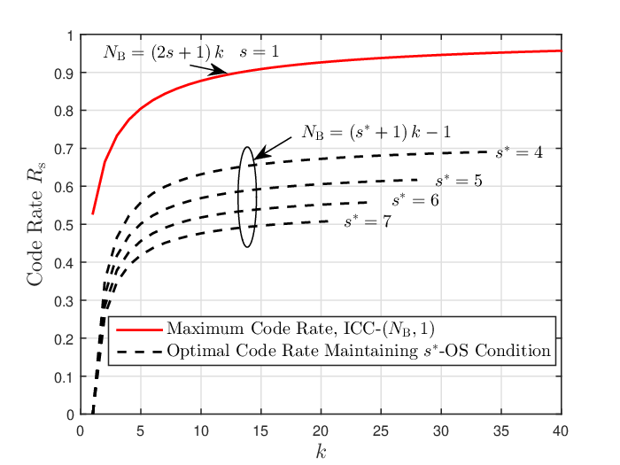
In Fig. 10 (b), we evaluate the code rate under the optimally-stable tradeoff. Before that, we consider the Eq. (9) for comparison and sketch the curve of maximum code rate under over . On this reference curve, the code rate increases and gradually approach 1 with the increase of . As to the optimally-stable tradeoff, we simulate the curves of code rate shown in Eq. (24) over from 4 to 7. As we can see, the code rate in this case is reduced compared with that without tradeoff consideration. With the increase of , we have to get less code rate. For example, the code rate under and thus is equal to 0.5083, which means the rate loss of 0.4205 (almost 45 percent) is caused by the tradeoff at this point.
VI-E CIR Estimation Under Optimally-Stable Tradeoff
Finally, we stimulate the performance of stable CIR estimation in Fig. 10 (c) where the NMSE is presented versus SNR of Bob under different number of antennas. and are respectively configured to be 6 and 256. Here, we consider the estimation using Eq. (12) and assume perfect identification for attacks. The performance under this type of estimator is not influenced by the specific value of due to the subspace projection property. We configure and do not consider the case where there is no attack since in this case LS estimator is a natural choice. For the simplicity of comparison, we only present the channel estimation under PTS attack because the estimation error floor under PTN and PTJ attack can be easily understood to be very high. The binned scheme proposed in [24] is simulated as an another comparison scheme. As we can see, PTS attack causes a high-NMSE floor on CIR estimation for Bob. This phenomenon can also be seen in the binned scheme. However, the estimation in our proposed framework breaks down this floor and its NMSE gradually decreases with the increase of transmitting antennas. Also, we consider perfect MMSE to be a performance benchmark for which perfect pilot tones, including Ava’s pilot tones, are assumed to be known by Alice. We find that the NMSE brought in our scheme gradually approaches the level under perfect MMSE with the increase of antennas. That’s because the asymptotically-optimal estimator highly relies on the statistical covariance matrix which is determined by the number of antennas.
VII Conclusions
This paper investigated the issue of pilot-aware attack on the uplink CTA in large-scale MISO-OFDM systems. We proposed a secure ICC-CTA protocol in which pilot tones, usually exposed in public, are now enabled to be shared between legitimate transceiver pair, with high security under hybrid attack environment. Theoretically, we discovered an critical fact that this architecture could exhibit a perfect security if the CPD model of mean AoA was considered. In practical scenarios with the DPD model of mean AoA, this architecture was required to make tradeoff between the security and stability of CIR estimation. We showed that given a suitable code rate, stable CIR estimation could be always maintained under a high security. We conclude this paper by pointing out some interesting topics for future work. As one interesting direction, more delicate optimization on the tradeoff could be further researched such that the code rate under optimally-stable tradeoff could be higher. The extension to solving the issue of pilot contamination in massive MIMO systems could be another interesting direction since the pilot phases guaranteed by our scheme can be superimposed onto the traditional optimized pilots and thus control even avoid pilot contamination in multi-cell scenarios with only three OFDM symbol time.
VIII Appendix
VIII-A Proof of Theorem 1
Since codewords in this constant-weight code are constrained to be with same and fixed length, the number of overlapping digits achieves its minimum only when the zero digits of each codeword are fully occupied. In this case, the remanent digits, i.e., the overlapping digits, account for which should be equal to and less than . Therefore, we can prove the theorem.
VIII-B Proof of Theorem 2
Considering the hybrid attack, we know that there exists the possibility of codewords to appear. Two interpreted codewords derived under and , if satisfying , will confuse Alice. In this case, each assumption is decided with the probability of . The possible number of codewords that satisfy this condition is equal to . One exception is when the codeword of Ava is identical to that of Bob. In this case, the codeword can be uniquely identified. Finally, there exists the possibility of codewords that could cause identification errors. Then the ultimate IEP can be proved.
VIII-C Proof of Proposition 3
Taking Bob for example, we can derive the estimation error as . Now let us focus on the term . We can express as where is the integrated CIR vector of i.i.d. random variables. Based on the Lemma B.26 in [33], is then transformed into . Here, the matrix satisfies . Therefore, we can derive at high SNR region. In the same way, we can derive . After calculating the matrix inverse and performing matrix multiplication, we can finally verify . This completes the proof.
VIII-D Proof of Theorem 3
Thanks to , the measure can be expressed as the equation satisfying . This equation can be expanded into with , and . By using the Lemma B.26 in [33] for each term, we can have . In the same way, we can obtain the relationship . As indicated in Proposition 3, there exists . By comparing the two simplified results of and , we can complete the proof.
VIII-E Proof of Theorem 4
First, we will prove . As shown in [22], the empirical CDF of eigenvalues of can be asymptotically approximated by the samples from . Therefore, the eigenvalues of different individuals, if overlapping at the same location, e.g., , can be approximated with the same eigenvalue. In this case, the ratio of two eigenvalues at the same location is one and therefore, we can prove for overlapping positions. Then we prove that there must . Examining and , we found that if is satisfied, there must exist since must have non-empty intersection with . In this case, the number of elements in is reduced to be smaller than that . Now we turn to the case in which we easily have and therefore the theorem is proved.
VIII-F Proof of Theorem 6
Let us determine the value of minimum of . From Eq. (23), we know that there exists and . Since , we can acquire as the minimum of . Note that it satisfies for . In this case, the value of will decrease with the increase of . Thus the maximum code rate, i.e. maximum security, can be achieved at this weight. Moreover, according to the Theorem 1, we can know there exists for an ICC- code and therefore we can derive the relationship between and . The theorem is finally proved.
References
- [1] T. E. Bogale and L. B. Le, “Massive MIMO and mmWave for 5G wireless HetNet: Potentials and challenges," IEEE Veh. Technol. Mag., vol. 11, no. 1, pp. 64-75, Feb. 2016.
- [2] Q. Yan, H. Zeng, T. Jiang, M. Li, W. Lou, and Y. T. Hou, “Jamming resilient communication using MIMO interference cancellation," IEEE Trans. Inf. Forensics Security, vol. 11, no. 7, pp. 1486-1499, Jul. 2016.
- [3] H. Rahbari, M. Krunz, and L. Lazos, “Swift jamming attack on frequency offset estimation: The Achilles�� Heel of OFDM systems," IEEE Trans. Mobile Comput., vol. 15, no. 5, pp. 1264-1278, May 2016.
- [4] C. Shahriar, M. La Pan, M. Lichtman, T. C. Clancy, R. McGwier, R. Tandon, S. Sodagari, and J. H. Reed, “PHY-Layer resiliency in OFDM communications: A tutorial," IEEE Commun. Surveys Tuts., vol. 17, no. 1, pp. 292-314, Aug. 2015.
- [5] H. Pirzadeh, S. M. Razavizadeh, and E. Bjornson, “Subverting massive MIMO by smart jamming," IEEE Wireless Commun. Lett., vol. 5, no. 1, pp. 20-23, Feb. 2016.
- [6] M. Lichtman, J. D. Poston, S. Amuru, C. Shahriar, T. C. Clancy, R. M. Buehrer, and J. H. Reed, “A communications jamming taxonomy," IEEE Security Privacy, vol. 14, no. 1, pp. 47-54, Jan. 2016.
- [7] M. Lichtman, R. P. Jover, M. Labib, R. Rao, V. Marojevic, and J. H. Reed, “LTE/LTE-A jamming, spoofing, and sniffing: Threat assessment and mitigation," IEEE Commun. Mag., vol. 54, no. 4, pp. 54-61, Apr. 2016.
- [8] T. C. Clancy, “Efficient OFDM denial: Pilot jamming and pilot nulling," in Proc. IEEE Int. Conf. Commun. (ICC), June 2011, pp. 1-5.
- [9] S. Sodagari and T. C. Clancy, “Efficient jamming attacks on MIMO channels," in Proc. IEEE Int. Conf. Commun. (ICC), June 2012, pp. 852-856.
- [10] D. Xu, P. Ren, Y. Wang, Q. Du, and L. Sun, “ICA-SBDC: a channel estimation and identification mechanism for MISO-OFDM systems under pilot spoofing attack," in Proc. IEEE Int. Conf. Commun. (ICC), May 2017, pp. 1-5.
- [11] W. Tu and L. Lai, “Keyless authentication and authenticated capacity,” IEEE Trans. Inf. Theory, vol. 64, no. 5, pp. 3696-3714, May 2018.
- [12] L. Lai, H. EI Gamal, and H. V. Poor, “Authentication over noisy channels,” IEEE Trans. Inf. Theory, vol. 55, no. 2, pp. 906-916, Feb. 2009.
- [13] P. L. Yu, J. S. Baras, and B. M. Sadler, “Physical-layer authentication,” IEEE Trans. Inf. Forensics and Security, vol. 3, no. 1, pp. 38-51, Mar. 2008.
- [14] Q. Peng, P. C. Cosman, and L. B. Milstein, “Spoofing or jamming: Performance analysis of a tactical cognitive radio adversary," IEEE J. Sel. Areas Commun., vol. 29, no. 4, pp. 903-911, Apr. 2011.
- [15] T. Doumi, M. F. Dolan, S. Tatesh, A. Casati, G. Tsirtsis, K. Anchan, and D. Flore, “LTE for public safety networks," IEEE Commun. Mag., vol. 51, no. 2, pp. 106-112, Feb. 2013.
- [16] X. Zhou, B. Maham, and A. Hjorungnes, “Pilot contamination for active eavesdropping," IEEE Trans. Wireless Commun., vol. 11, no. 3, pp. 903-907, Mar. 2012.
- [17] D. Kapetanovic, G. Zheng, K.-K. Wong, and B. Ottersten, “Detection of pilot contamination attack using random training and massive MIMO," in Proc. IEEE Int. Symp. on Personal, Indoor and Mobile Radio Commun. (PIMRC’13), Sep. 2013, pp. 13-18.
- [18] Q. Xiong, Y.-C. Liang, K. H. Li and Y. Gong, “An energy-ratio-based approach for detecting pilot spoofing attack in multiple-antenna systems,” IEEE Trans. Inf. Forensics and Security, vol. 10, no. 5, pp. 932-940, May 2015.
- [19] J. K. Tugnait, “On mitigation of pilot spoofing attack,” in Proc. 2017 IEEE Int. Conf. Acous. Speech Signal Proc., Mar. 2017, pp. 2097-2101.
- [20] D. Kapetanovic, A. Al-Nahari, A. Stojanovic, and F. Rusek, “Detection of active eavesdroppers in massive MIMO,” in Proc. IEEE Int. Symp. on Personal Indoor and Mobile Radio Commun. (PIMRC’14), Sep. 2014, pp. 585-589.
- [21] J.-M. Kang, C. In, and H. M. Kim, “Detection of pilot contamination attack for multi-antenna based secrecy systems,” in Proc. IEEE Vehicular Technology Conf. (VTC Spring), May 2015, pp. 1-5.
- [22] A. Adhikary, J. Nam, J.-Y. Ahn, and G. Caire, “Joint spatial division and multiplexing-The large-scale array regime,,” IEEE Trans. Inf. Theory, vol. 59, no. 10, pp. 6441-6463, Oct. 2013.
- [23] T. C. Clancy and N.Georgen, “Security in cognitive radio networks: threats and mitigations," in Proc. 3rd Int. Conf. CrownCom., May 2008, pp. 1-8.
- [24] C. Shahriar and T. C. Clancy, “Performance impact of pilot tone randomization to mitigate OFDM jamming attacks," in Proc. IEEE CCNC, Jan. 2013, pp. 813-816.
- [25] D. Tse and P. Viswanath, Fundamentals of Wireless Communication. Cambridge, U.K.: Cambridge Univ. Press, 2005.
- [26] D. Xu, P. Ren, and J. A. Ritcey, “Optimal independence-checking coding for secure uplink training in large-scale MISO-OFDM systems," accepted in Proc. IEEE Int. Conf. Commun. (ICC) 2018.
- [27] Q. Yan, H. Zeng, T. Jiang, M. Li, W. Lou, and Y. T. Hou, “MIMO based jamming resilient communication in wireless networks," in IEEE INFOCOM��14, Apr. 2014, pp. 2697-2706.
- [28] M. Abdelhakim, J. Ren, and T. Li, “Reliable OFDM system design under hostile multi-tone jamming," in Proc. IEEE Global Commun. Conf. (GLOBECOM), Dec. 2012, pp. 4290-4295.
- [29] B. Han and Y. R. Zheng, “Higher rank principal Kronecker model for triply selective fading channels with experimental validation," IEEE Trans. Veh. Technol., vol. 64, no. 5, pp. 1654-1663, May 2015.
- [30] R. Bhagavatula and R. W. Heath Jr., “Computing the receive spatial correlation for a multi-cluster MIMO channel using different array configurations,” in Proc. IEEE Global Commun. Conf. (GLOBECOM), Dec. 2008, pp. 3959-3963.
- [31] M. R. McKay, P. J. Smith, H. A. Suraweera, and I. B. Collings, “On the mutual information distribution of OFDM-based spatial multiplexing: exact variance and outage approximation," IEEE Trans. Inf. Theory, vol. 54, no. 7, pp. 3260-3278, July 2008.
- [32] M. Z. Shakir, A. Rao, and M. Alouini, “On the decision threshold of eigenvalue ratio detector based on moments of joint and marginal distributions of extreme eigenvalues,” IEEE Trans. Wireless Commun., vol. 12, no. 3, pp. 974-983, Mar. 2013.
- [33] Z. D. Bai and J. W. Silverstein, Spectral Analysis of Large Dimensional Random Matrices, 2nd ed. Springer Series in Statistics, New York, NY, USA, 2009.