Understanding Geometry of Encoder-Decoder CNNs

Jong Chul Ye Affiliation: Dept. of Bio/Brain Engineering, KAIST Daejeon 34141, Republic of Korea. Affiliation: Dept. of Mathematical Sciences, KAIST, Daejeon 34141, Republic of Korea. Correspondence to: jong.ye@gmail.com Woon Kyoung Sung Affiliation: Dept. of Mathematical Sciences, KAIST, Daejeon 34141, Republic of Korea.

Abstract

Encoder-decoder networks using convolutional neural network (CNN) architecture have been extensively used in deep learning literatures thanks to its excellent performance for various inverse problems. However, it is still difficult to obtain coherent geometric view why such an architecture gives the desired performance. Inspired by recent theoretical understanding on generalizability, expressivity and optimization landscape of neural networks, as well as the theory of deep convolutional framelets, here we provide a unified theoretical framework that leads to a better understanding of geometry of encoder-decoder CNNs. Our unified framework shows that encoder-decoder CNN architecture is closely related to nonlinear frame representation using combinatorial convolution frames, whose expressibility increases exponentially with the depth. We also demonstrate the importance of skipped connection in terms of expressibility, and optimization landscape.

Keywords:

Encoder-decoder network, expressivity, generalizability, optimization landscape, convolution framelets

marginparsep has been altered.
topmargin has been altered.
marginparwidth has been altered.
marginparpush has been altered.

The page layout violates the ICML style.

Please do not change the page layout, or include packages like geometry, savetrees, or fullpage, which change it for you.

We’re not able to reliably undo arbitrary changes to the style. Please remove the offending package(s), or layout-changing commands and try again.

1 Introduction

For the last decade, we have witnessed the unprecedented success of deep neural networks (DNN) in various applications in computer vision, classification, medical imaging, etc. Aside from traditional applications such as classification (Krizhevsky et al. 2012), segmentation (Ronneberger et al. 2015), image denoising (Zhang et al. 2017), super-resolution (Kim et al. 2016), etc, deep learning approaches have already become the state-of-the-art technologies in various inverse problems in x-ray CT, MRI, etc (Kang et al. 2017; Jin et al. 2017; Hammernik et al. 2018)

However, the more we see the success of deep learning, the more mysterious the nature of deep neural networks becomes. In particular, the amazing aspects of expressive power, generalization capability, and optimization landscape of DNNs have become an intellectual challenge for machine learning community, leading to many new theoretical results with varying capacities to facilitate the understanding of deep neural networks (Ge & Ma 2017; Hanin & Sellke 2017; Yarotsky 2017; Nguyen & Hein 2017; Arora et al. 2016; Du et al. 2018; Raghu et al. 2017; Bartlett et al. 2017; Neyshabur et al. 2018; Nguyen & Hein 2018; Rolnick & Tegmark 2017; Shen 2018).

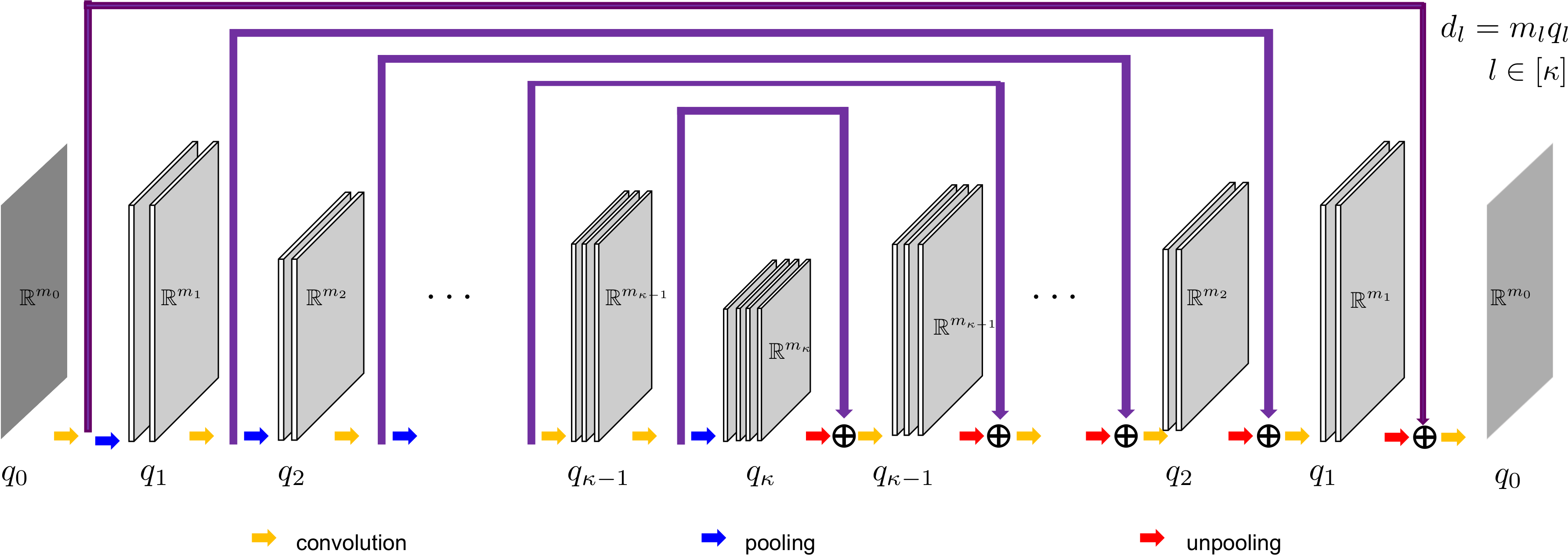
Refer to caption — Figure 1: An architecture of $\kappa$ -layer symmetric encoder-decoder CNN with skipped connections. Here, $q_{l}$ denotes the number of channels at the $l$ -th layer, whereas $m_{l}$ refers to each channel dimension, and $d_{l}$ represents the total dimension of the feature at the $l$ -th layer.

In inverse problems, one of the most widely employed network architectures is so-called encoder-decoder CNN architectures (Ronneberger et al. 2015). In contrast to the simplified form of the neural networks that are often used in theoretical analysis, these encoder-decoder CNNs usually have more complicated network architectures such as symmetric network configuration, skipped connections, etc. Therefore, it is not clear how the aforementioned theory can be used to understand the geometry of encoder-decoder CNNs to examine the origin of their superior performance.

Recently, the authors in (Ye et al. 2018) proposed so-called deep convolutional framelets to explain the encoder-decoder CNN architecture from a signal processing perspective. The main idea is that a data-driven decomposition of Hankel matrix constructed from the input data provides encoder-decoder layers that have striking similarity to the encoder-decoder CNNs. However, one of the main weaknesses of the theory is that it is not clear where the exponential expressiveness comes from. Moreover, many theoretical issues of neural networks such as generalizability and the optimization landscape, which have been extensively studied in machine learning literature, have not been addressed.

Therefore, this work aims at filling the gap and finding the connections between machine learning and signal processing to provide a unified theoretical analysis that facilitates the geometric understanding of encoder-decoder CNNs. Accordingly, we have revealed the following geometric features of encoder-decoder CNNs:

•

An encoder-decoder CNN with an over-parameterized feature layer approximates a map between two smooth manifolds that is decomposed as a high-dimensional embedding followed by a quotient map.
•

An encoder-decoder CNN with ReLU nonlinearity can be understood as deep convolutional framelets that use combinatorial frames of spatially varying convolutions. Accordingly, the number of linear representations increases exponentially with the network depth. This also suggests that the input space is divided into non-overlapping areas where each area shares the common linear representation.
•

We derive an explicit form of the Lipschitz condition that determines the generalization capability of the encoder-decoder CNNs. The expression shows that the expressiveness of the network is not affected by the control of the Lipschitz constant.
•

We provide explicit conditions under which the optimization landscape for encoder-decoder CNNs is benign. Specifically, we show that the skipped connection play important roles in smoothing out the optimization landscape.

All the proof of the theorems and lemmas in this paper are included in the Supplementary Material.

2 Related Works

Choromanska et al (Choromanska et al. 2015) employed the spin glass model from statistical physics to analyze the representation power of deep neural networks. Telgarsky constructs interesting classes of functions that can be only computed efficiently by deep ReLU nets, but not by shallower networks with a similar number of parameters (Telgarsky 2016). Arora et al (Arora et al. 2016) showed that for every natural number $k$ there exists a ReLU network with $k^{2}$ hidden layers and total size of $k^{2}$ , which can be represented by $\frac{1}{2}k^{k+1}-1$ neurons with at most $k$ -hidden layers. All these results agree that the expressive power of deep neural networks increases exponentially with the network depth.

The generalization capability have been addressed in terms of various complexity measures such as Rademacher complexity (Bartlett & Mendelson 2002), VC bound (Anthony & Bartlett 2009), Kolmorogov complexity (Schmidhuber 1997), etc. However, a recent work (Zhang et al. 2016) showed intriguing results that these classical bounds are too pessimistic to explain the generalizability of deep neural networks. Moreover, it has been repeatedly shown that over-parameterized deep neural networks, which are trained with fewer samples than the number of neurons, generalize well rather than overfitting (Cohen et al. 2018; Wei et al. 2018; Brutzkus et al. 2017; Du & Lee 2018), which phenomenon cannot be explained by the classical complexity results.

The optimization landscape of neural networks have been another important theoretical issue in neural networks. Originally observed in linear deep neural networks (Kawaguchi 2016), the benign optimization landscape has been consistently observed in various neural networks (Du et al. 2018; Nguyen & Hein 2018; Du et al. 2017; Nguyen & Hein 2017).

However, these theoretical works mainly focus on simplified network architectures, and we are not aware of analysis for encoder-decoder CNNs.

3 Encoder-Decoder CNNs

3.1 Definition

In this section, we provide a formal definition of encoder-decoder CNNs (E-D CNNs) to facilitate the theoretical analysis. Although our definition is for 1-dimensional signals, its extension to 2-D images is straightforward.

3.1.1 Basic Architecture

Consider encoder-decoder networks in Fig. 1. Specifically, the encoder network maps a given input signal $x\in\boldsymbol{\mathcal{X}}\subset{\mathbb{R}}^{d_{0}}$ to a feature space $z\in\boldsymbol{\mathcal{Z}}\subset{\mathbb{R}}^{d_{\kappa}}$ , whereas the decoder takes this feature map as an input, process it and produce an output $y\in\boldsymbol{\mathcal{Y}}\subset{\mathbb{R}}^{d_{L}}$ . In this paper, symmetric configuration is considered so that both encoder and decoder have the same number of layers, say $\kappa$ ; the input and output dimensions for the encoder layer ${\mathcal{E}}^{l}$ and the decoder layer ${\mathcal{D}}^{l}$ are symmetric:

\displaystyle{\mathcal{E}}^{l}:{\mathbb{R}}^{d_{l-1}}\mapsto{\mathbb{R}}^{d_{l}},\quad{\mathcal{D}}^{l}:{\mathbb{R}}^{d_{l}}\mapsto{\mathbb{R}}^{d_{l-1}}

where $l\in[\kappa]$ with $[n]$ denoting the set $\{1,\cdots,n\}$ ; and both input and output dimension is $d_{0}$ . More specifically, the $l$ -th layer input signal for the encoder layer comes from $q_{l-1}$ number of input channels:

\xi^{l-1}=\begin{bmatrix}\xi_{1}^{l-1\top}&\cdots&\xi^{l-1\top}_{q_{l-1}}\end{bmatrix}^{\top}\in{\mathbb{R}}^{d_{l-1}},\quad

where ^⊤ denotes the transpose, and $\xi_{j}^{l-1}\in{\mathbb{R}}^{m_{l-1}}$ refers to the $j$ -th channel input with the dimension $m_{l-1}$ . Therefore, the overall input dimension is given by $d_{l-1}:={m_{l-1}q_{l-1}}$ . Then, the $l$ -th layer encoder generates $q_{l}$ channel output using the convolution operation:

\displaystyle\xi_{j}^{l}=\sigma\left(\Phi^{l\top}\sum_{k=1}^{q_{l-1}}\left(\xi_{k}^{l-1}\circledast\overline{\psi}_{j,k}^{l}\right)\right),~j\in[q_{l}]

(1)

where $\xi_{j}^{l}\in{\mathbb{R}}^{m_{l}}$ refers to the $j$ -th channel output after the convolutional filtering with the $r$ -tap filters $\overline{\psi}_{j,k}^{l}\in{\mathbb{R}}^{r}$ and pooling operation $\Phi^{l\top}\in{\mathbb{R}}^{m_{l}\times m_{l-1}}$ , and $\sigma(\cdot)$ denotes the element wise rectified linear unit (ReLU). More specifically, $\overline{\psi}_{j,k}^{l}\in{\mathbb{R}}^{r}$ denotes the $r$ -tap convolutional kernel that is convolved with the $k$ -th input to contribute to the output of the $j$ -th channel, $\circledast$ is the circular convolution via periodic boundary condition to avoid special treatment of the convolution at the boundary, and $\overline{v}$ refers to the flipped version of the vector $v$ . For the formal definition of the convolution operation used in this paper, see Appendix A in Supplementary Material.

Moreover, as shown in Appendix B in Supplementary Material, an equivalent matrix representation of the encoder layer is then given by

\displaystyle\xi^{l}:=\sigma(E^{l\top}\xi^{l-1})=\begin{bmatrix}\xi^{l\top}_{1}&\cdots&\xi^{l\top}_{q_{l}}\end{bmatrix}^{\top}

where $E^{l}\in{\mathbb{R}}^{d_{l-1}\times d_{l}}$ is computed by¹¹ 1 Here, without loss of generality, bias term is not explicitly shown, since it can be incorporated into the matrix $E^{l}$ and $D^{l}$ as an additional column.

\displaystyle E^{l}=\begin{bmatrix}\Phi^{l}\circledast\psi^{l}_{1,1}&\cdots&\Phi^{l}\circledast\psi^{l}_{q_{l},1}\\ \vdots&\ddots&\vdots\\ \Phi^{l}\circledast\psi^{l}_{1,q_{l-1}}&\cdots&\Phi^{l}\circledast\psi^{l}_{q_{l},q_{l-1}}\end{bmatrix}

(2)

with

\displaystyle\begin{bmatrix}\Phi^{l}\circledast\psi_{i,j}^{l}\end{bmatrix}:=\begin{bmatrix}\phi^{l}_{1}\circledast\psi_{i,j}^{l}&\cdots&\phi^{l}_{m_{l}}\circledast\psi_{i,j}^{l}\end{bmatrix}

(3)

On the other hand, the $l$ -th layer input signal for the decoder layer comes from $q_{l}$ channel inputs, i.e. $\tilde{\xi}^{l}=\begin{bmatrix}\tilde{\xi}_{1}^{l\top}&\cdots&\tilde{\xi}^{l}_{q_{l}\top}\end{bmatrix}^{\top}\in{\mathbb{R}}^{d_{l}},$ and the decoder layer convolution is given by

\displaystyle\tilde{\xi}_{j}^{l-1}=\sigma\left(\sum_{k=1}^{q_{l}}\left(\tilde{\Phi}^{l}\tilde{\xi}^{l}_{k}\circledast{\tilde{\psi}_{j,k}^{l}}\right)\right),\quad j\in[q_{l-1}]

(4)

where the unpooling layer is denoted by $\tilde{\Phi}^{l}\in{\mathbb{R}}^{m_{l-1}\times m_{l}}$ . Note that (1) and (4) differ in their order of the pooling or unpooling layers. Specifically, a pooling operation is applied after the convolution at the encoder layer, whereas, at the decoder, an unpooling operation is performed before the convolution to maintain the symmetry of the networks. In matrix form, a decoder layer is given by

\displaystyle\tilde{\xi}^{l-1}:=\sigma(D^{l}\tilde{\xi}^{l})=\begin{bmatrix}\tilde{\xi}^{l-1\top}_{1}&\cdots&\tilde{\xi}^{l-1\top}_{q_{l-1}}\end{bmatrix}^{\top}\

where $D^{l}\in{\mathbb{R}}^{d_{l}\times d_{l-1}}$ is computed by

\displaystyle D^{l}=\begin{bmatrix}\tilde{\Phi}^{l}\circledast\tilde{\psi}^{l}_{1,1}&\cdots&\tilde{\Phi}^{l}\circledast\tilde{\psi}^{l}_{1,q_{l}}\\ \vdots&\ddots&\vdots\\ \tilde{\Phi}^{l}\circledast\tilde{\psi}^{l}_{q_{l-1},1}&\cdots&\tilde{\Phi}^{l}\circledast\tilde{\psi}^{l}_{q_{l-1},q_{l}}\end{bmatrix}

(5)

3.1.2 E-D CNN with skipped connection

As shown in Fig. 1, a skipped connection is often used to bypass an encoder layer output to a decoder layer. The corresponding filtering operation at the $l$ -th layer encoder is described by

\displaystyle\begin{bmatrix}\xi_{j}^{l}\\ \chi_{j}^{l}\end{bmatrix}=\begin{bmatrix}\sigma\left(\Phi^{l\top}\sum_{k=1}^{q_{l-1}}\left(\xi_{k}^{l-1}\circledast\overline{\psi}_{j,k}^{l}\right)\right)\\ \sigma\left(\sum_{k=1}^{q_{l-1}}\left(\xi_{k}^{l-1}\circledast\overline{\psi}_{j,k}^{l}\right)\right)\end{bmatrix}

(6)

where $\chi_{j}^{l}$ and $\xi_{j}^{l}$ denote the skipped output, and the pooled output via $\Phi^{l\top}$ , respectively, after the filtering with $\overline{\psi}_{j,k}$ . As shown in Fig. 1, the skipped branch is no more filtered at the subsequent layer, but is merged at the symmetric decoder layer:

\displaystyle\tilde{\xi}_{j}^{l-1}=\sigma\left(\sum_{k=1}^{q_{l}}\left((\tilde{\Phi}^{l}\tilde{\xi}^{l}_{k}+\chi^{l}_{k})\circledast{\tilde{\psi}_{j,k}^{l}}\right)\right)

In matrix form, the encoder layer with the skipped connection can be represented by

{\mathcal{E}}^{l}:\xi^{l-1}\mapsto\begin{bmatrix}\xi^{l\top}&\chi^{l\top}\end{bmatrix}^{\top}

where

\displaystyle\xi^{l}:=\sigma(E^{l\top}\xi^{l-1})

\displaystyle\chi^{l}:=\sigma(S^{l\top}\xi^{l-1})

(7)

where $E^{l}$ is given in (2) and the skipped branch filter matrix $S^{l}$ is represented by

\displaystyle S^{l}=\begin{bmatrix}I_{m_{l-1}}\circledast\psi^{l}_{1,1}&\cdots&I_{m_{l-1}}\circledast\psi^{l}_{q_{l},1}\\ \vdots&\ddots&\vdots\\ I_{m_{l-1}}\circledast\psi^{l}_{1,q_{l-1}}&\cdots&I_{m_{l-1}}\circledast\psi^{l}_{q_{l},q_{l-1}}\end{bmatrix}

(8)

where $I_{m_{l-1}}$ denotes the $m_{l-1}\times m_{l-1}$ identity matrix. This implies that we can regard the skipped branch as the identity pooling $I_{m_{l-1}}$ applied to the filtered signals. Here, we denote the output dimension of the skipped connection as

s_{l}:=m_{l-1}q_{l}\quad.

Then, the skipped branch at the $l$ -th encoder layer is merged at the $l$ -th decoder layer, which is defined as

{\mathcal{D}}^{l}:\begin{bmatrix}\tilde{\xi}^{l\top}&\chi^{l\top}\end{bmatrix}^{\top}\mapsto\tilde{\xi}^{l-1}

where

\displaystyle\tilde{\xi}^{l-1}:=\sigma(D^{l}\tilde{\xi}^{l}+\tilde{S}^{l}\chi^{l})

(9)

and $D^{l}$ is defined in (5), and $\tilde{S}^{l}$ is given by

\displaystyle\tilde{S}^{l}=\begin{bmatrix}I_{m_{l-1}}\circledast\tilde{\psi}^{l}_{1,1}&\cdots&I_{m_{l-1}}\circledast\tilde{\psi}^{l}_{1,q_{l}}\\ \vdots&\ddots&\vdots\\ I_{m_{l-1}}\circledast\tilde{\psi}^{l}_{q_{l-1},1}&\cdots&I_{m_{l-1}}\circledast\tilde{\psi}^{l}_{q_{l-1},q_{l}}\end{bmatrix}

(10)

3.2 Parameterization of E-D CNNs

At the $l$ -th encoder (resp. decoder) layer, there are $q_{l}q_{l-1}$ filter set that generates the $q_{l}$ (resp. $q_{l-1}$ ) output channels from $q_{l-1}$ (resp. $q_{l}$ ) input channels. In many CNNs, the filter lengths are set to equal across the layer. In our case, we set this as $r$ , so the number of filter coefficients for the $l$ -layer is

n_{l}:=rq_{l}q_{l-1},\quad l\in[\kappa]

These parameters should be estimated during the training phase. Specifically, by denoting the set of all parameter matrices $\boldsymbol{\mathcal{W}}=\boldsymbol{\mathcal{W}}_{E}\times\boldsymbol{\mathcal{W}}_{D}$ where $\boldsymbol{\mathcal{W}}_{E}:={\mathbb{R}}^{n_{\kappa}}\times\cdots\times{\mathbb{R}}^{n_{1}}$ and $\boldsymbol{\mathcal{W}}_{D}:={\mathbb{R}}^{n_{1}}\times\cdots\times{\mathbb{R}}^{n_{\kappa}}$ , we compose all layer-wise maps to define an encoder-decoder CNN as

\displaystyle z=F({\mathbf{W}},x).

(11)

Regardless of the existence of skipped connections, note that the same number of unknown parameters is used because the skipped connection uses the same set of filters.

4 Theoretical Analysis of E-D CNNs

4.1 Differential Topology

First, we briefly revisit the work by Shen (Shen 2018), which gives an topological insight on the E-D CNNs.

Proposition 1 (Extension of Theorem 3 in (Shen 2018)).

Let $f:\boldsymbol{\mathcal{X}}\mapsto\boldsymbol{\mathcal{Y}}\subset{\mathbb{R}}^{q}$ be a continuous map of smooth manifolds such that $f=g\circ h$ , where $g:{\mathbb{R}}^{p}\mapsto{\mathbb{R}}^{q}$ with $p\geq q$ is a Lipschitz continuous map. If $p>2\dim\boldsymbol{\mathcal{X}}$ , then there exists a smooth embedding $\tilde{h}:\boldsymbol{\mathcal{X}}\mapsto{\mathbb{R}}^{p}$ , so that the following inequality holds true for a chosen norm and all $x\in\boldsymbol{\mathcal{X}}$ and $\epsilon>0$ :

\|f(x)-g\circ\tilde{h}(x)\|\leq\epsilon

Here, $p>2\dim\boldsymbol{\mathcal{X}}$ comes from the weak Whitney embedding theorem (Whitney 1936; Tu 2011). Note that Theorem 1 informs that a neural network, designed as a continuous map of smooth manifolds, can be considered as an approximation of a task map that is composed of a smooth embedding followed by an additional map. In fact, this decomposition is quite general for a map between smooth manifolds as shown in the following proposition:

Proposition 2.

(Shen 2018) Let $f:\boldsymbol{\mathcal{X}}\mapsto\boldsymbol{\mathcal{Y}}\subset{\mathbb{R}}^{q}$ be a map of smooth manifolds, then the task $f$ admits a decomposition of $f=g\circ h$ , where $h:\boldsymbol{\mathcal{X}}\mapsto\boldsymbol{\mathcal{Z}}\subset{\mathbb{R}}^{p}$ with $p\geq 2\dim\boldsymbol{\mathcal{X}}$ is a smooth embedding. Furthermore, the task map $f$ is a quotient map, if and only if the map $g$ is a quotient map.

To understand the meaning of the last sentence in Proposition 2, we briefly review the concept of the quotient space and quotient map (Tu 2011). Specifically, let $\sim$ be an equivalence relation on $\boldsymbol{\mathcal{X}}$ . Then, the quotient space, $\boldsymbol{\mathcal{Y}}=\boldsymbol{\mathcal{X}}/\sim$ is defined to be the set of equivalence classes of elements of $\boldsymbol{\mathcal{X}}$ . For example, we can declare images perturbed by noises as an equivalent class such that our quotient map is designed to map the noisy signals to its noiseless equivalent image.

It is remarkable that Proposition 1 and Proposition 2 give interpretable conditions for design parameters such as network width (i.e. no of channels), pooling layers, etc. For example, if there are no pooling layers, the dimensionality conditions in Proposition 1 and Proposition 2 can be easily met in practice by increasing the number of channels more than twice the input channels. With the pooling layers, one could calculate the number of channels in a similar way. In general, Proposition 1 and Proposition 2 strongly suggest an encoder-decoder architecture with the constraint $d_{0}\leq d_{1}\leq\cdots\leq d_{\kappa}$ with $d_{\kappa}>2d_{0}$ , where an encoder maps an input signal to higher dimensional feature space whose dimension is at least twice bigger than the input space. Then, the decoder determines the nature of the overall neural network.

4.2 Links to the frame representation

One of the important contributions of recent theory of deep convolutional framelets (Ye et al. 2018) is that encoder-decoder CNNs have an interesting link to multi-scale convolution framelet expansion. To see this, we first define filter matrices $\Psi^{l}\in{\mathbb{R}}^{rq_{l-1}\times q_{l}}$ and $\tilde{\Psi}^{l}\in{\mathbb{R}}^{rq_{l-1}\times q_{l}}$ for encoder and decoder:

\Psi^{l}:=\begin{bmatrix}\psi^{l}_{1,1}&\cdots&\psi^{l}_{q_{l},1}\\ \vdots&\ddots&\vdots\\ \psi^{l}_{1,q_{l-1}}&\cdots&\psi^{l}_{q_{l},q_{l-1}}\end{bmatrix}

\tilde{\Psi}^{l}:=\begin{bmatrix}\tilde{\psi}^{l}_{1,1}&\cdots&\tilde{\psi}^{l}_{1,q_{l}}\\ \vdots&\ddots&\vdots\\ \tilde{\psi}^{l}_{q_{l-1},1}&\cdots&\tilde{\psi}^{l}_{q_{l-1},q_{l}}\end{bmatrix}

Then, the following proposition, which is novel and significantly extended from (Ye et al. 2018), states the importance of the frame conditions for the pooling layers and filters to obtain convolution framelet expansion (Yin et al. 2017).

Proposition 3.

Consider an encoder-decoder CNN without ReLU nonlinearities. Let $\Phi^{l\top}$ and $\tilde{\Phi}^{l}$ denote the $l$ -th encoder and decoder layer pooling layers, respectively, and $\Psi^{l}$ and $\tilde{\Psi}^{l}$ refer to the encoder and decoder filter matrices. Then, the following statements are true.

1) For the encoder-decoder CNN without skipped connection, if the following frame conditions are satisfied for all $l\in[\kappa]$

\displaystyle\tilde{\Phi}^{l}\Phi^{l\top}=\alpha I_{m_{l-1}},~\Psi^{l}\tilde{\Psi}^{l\top}=\frac{1}{r\alpha}I_{rq_{l-1}}

(12)

then we have

\displaystyle x

\displaystyle=

\displaystyle\sum_{i}\langle b_{i},x\rangle\tilde{b}_{i}

(13)

where $b_{i}$ and $\tilde{b}_{i}$ denote the $i$ -th column of the following frame basis and its dual:

	$\displaystyle B$	$\displaystyle=$	$\displaystyle E^{1}E^{2}\cdots E^{\kappa},~\quad$		(14)
	$\displaystyle\tilde{B}$	$\displaystyle=$	$\displaystyle D^{1}D^{2}\cdots D^{\kappa}$		(15)

2) For the encoder-decoder CNN with skipped connection, if the following frame conditions are satisfied for all $l\in[\kappa]$ :

\displaystyle\tilde{\Phi}^{l}\Phi^{l\top}=\alpha I_{m_{l-1}},~\Psi^{l}\tilde{\Psi}^{l\top}=\frac{1}{r(\alpha+1)}I_{rq_{l-1}}

(16)

then (13) holds, where $b_{i}$ and $\tilde{b}_{i}$ denote the $i$ -th column of the following frame and its duals:

\displaystyle B^{skp}\quad(\in{\mathbb{R}}^{d_{0}\times(d_{\kappa}+\sum_{l=1}^{\kappa}s_{l}}))

(17)

:=\begin{bmatrix}E^{1}\cdots E^{\kappa}&E^{1}\cdots E^{\kappa-1}S^{\kappa}&\cdots&E^{1}S^{2}&S^{1}\end{bmatrix}

\displaystyle\tilde{B}^{skp}\quad(\in{\mathbb{R}}^{d_{0}\times(d_{\kappa}+\sum_{l=1}^{\kappa}s_{l}}))

(18)

:=\begin{bmatrix}D^{1}\cdots D^{\kappa}&D^{1}\cdots D^{\kappa-1}\tilde{S}^{\kappa}&\cdots&D^{1}\tilde{S}^{2}&\tilde{S}^{1}\end{bmatrix}

Furthermore, the following corollary shows that the total basis and its dual indeed come from multiple convolutional operations across layers:

Corollary 4.

If there exist no pooling layers, then the $t$ -th block of the frame basis matrix for $t\in[q_{l}]$ is given by

\left[E^{1}\cdots E^{l}\right]_{t}=\left[E^{1}\cdots E^{l-1}S^{l}\right]_{t}

=I_{m}\circledast\left(\sum_{j_{l-1},\cdots,j_{1}=1}^{q_{l-1},\cdots,q_{1}}\psi_{j_{1},1}^{l}\circledast\cdots\circledast\psi_{t,j_{l-1}}^{l}\right)

Similarly,

\left[D^{1}\cdots D^{l}\right]_{t}=\left[D^{1}\cdots D^{l-1}\tilde{S}^{l}\right]_{t}

=I_{m}\circledast\left(\sum_{j_{l-1},\cdots,j_{1}=1}^{q_{l-1},\cdots,q_{1}}\tilde{\psi}_{j_{1},1}^{l}\circledast\cdots\circledast{\tilde{\psi}}_{t,j_{l-1}}^{l}\right)

This suggests that the length of the convolutional filters increases with the depth by cascading multiple convolution operations across the layers. While Proposition 3 informs that the skipped connection increases the dimension of the feature space from $d_{\kappa}$ to $d_{\kappa}+\sum_{l=1}^{\kappa}s_{l}$ , Corollary 4 suggest that the cascaded expression of the filters becomes more diverse for the case of encoder-decoder CNNs with skipped connection. Specifically, instead of convolving all $\kappa$ layers of filters, the skipped connection allows the combination of subset of filters. All these make the frame representation from skipped connection more expressive.

4.3 Expressiveness

However, to satisfy the frame conditions (12) or (16), we need $q_{l}\geq rq_{l-1}$ so that the number of output filter channel $q_{l}$ should increase exponentially. While this condition can be relaxed when the underlying signal has low-rank Hankel matrix structure (Ye et al. 2018), the explicit use of the frame condition is still rarely observed. Moreover, in contrast to the classical wavelet analysis, the perfect reconstruction condition itself is not interesting in neural networks, since the output of the network should be different from the input due to the task dependent processing.

Here, we claim that one of the important roles of using ReLU is that it allows combinatorial basis selection such that exponentially large number of basis expansion is feasible once the network is trained. This is in contrast with the standard framelet basis estimation. For example, for a given target data $Y=\begin{bmatrix}y^{(1)}&\cdots&y^{(T)}\end{bmatrix}$ and the input data $X=\begin{bmatrix}x^{(1)}&\cdots&x^{(T)}\end{bmatrix}$ , the estimation problem of the frame basis and its dual in Proposition 3 is optimal for the given training data, but the network is not expressive and does not generalize well when the different type of input data is given. Thus, one of the important requirements is to allow large number of expressions that are adaptive to the different inputs.

Indeed, ReLU nonlinearity makes the network more expressive. For example, consider a trained two layer encoder-decoder CNN:

\displaystyle y=\tilde{B}\Lambda(x)B^{\top}x

(19)

where $\tilde{B}\in{\mathbb{R}}^{d_{0}\times d_{1}}$ and $B\in{\mathbb{R}}^{d_{0}\times d_{1}}$ and $\Lambda(x)$ is a diagonal matrix with 0, 1 elements that are determined by the ReLU output. Now, the matrix can be equivalently represented by

\displaystyle\tilde{B}\Lambda(x)B^{\top}=\sum_{i=1}^{d_{1}}\sigma_{i}(x)\tilde{b}_{i}b_{i}^{\top}

(20)

where $\sigma_{i}(x)$ refers to the $(i,i)$ -th diagonal element of $\Lambda(x)$ . Therefore, depending on the input data $x\in{\mathbb{R}}^{d_{0}}$ , $\sigma_{i}(x)$ is either 0 or 1 so that a maximum $2^{d_{1}}$ distinct configurations of the matrix can be represented using (20), which is significantly more expressive than using the single representation with the frame and its dual. This observation can be generalized as shown in Theorem 5.

Theorem 5 (Expressiveness of encoder-decoder networks).

Let

	$\displaystyle\tilde{\Upsilon}^{l}=\tilde{\Upsilon}^{l}(x):=\tilde{\Upsilon}^{l-1}\tilde{\Lambda}^{l}(x)D^{l},~$		(21)
	$\displaystyle\Upsilon^{l}=\Upsilon^{l}(x):=\Upsilon^{l-1}E^{l}\Lambda^{l}(x),~$		(22)

with $\tilde{\Upsilon}^{0}(x)=I_{d_{0}}$ and $\Upsilon^{0}(x)=I_{d_{0}}$ , and

	$\displaystyle M^{l}=M^{l}(x):=S^{l}\Lambda_{S}^{l}(x)$		(23)
	$\displaystyle\tilde{M}^{l}=\tilde{M}^{l}(x):=\tilde{\Lambda}^{l}(x)\tilde{S}^{l}$		(24)

where $\Lambda^{l}(x)$ and $\tilde{\Lambda}^{l}(x)$ refer to the diagonal matrices from ReLU at the $l$ -th layer encoder and decoder, respectively, which have 1 or 0 values; $\Lambda_{S}^{l}(x)$ refers to a similarly defined diagonal matrices from ReLU at the $l$ -th skipped branch of encoder. Then, the following statements are true.

1) Under ReLUs, an encoder-decoder CNN without skipped connection can be represented by

\displaystyle y=\tilde{\mathcal{B}}(x){\mathcal{B}}^{\top}(x)x=\sum_{i}\langle x,b_{i}(x)\rangle\tilde{b}_{i}(x)

(25)

where

\displaystyle{\mathcal{B}}(x)=\Upsilon^{\kappa}(x)

\displaystyle\tilde{\mathcal{B}}(x)=\tilde{\Upsilon}^{\kappa}(x)

(26)

Furthermore, the maximum number of available linear representation is given by

\displaystyle N_{rep}=2^{\sum_{i=1}^{\kappa}d_{i}-d_{\kappa}},\quad

(27)

2) An encoder-decoder CNN with skipped connection under ReLUs is given by

\displaystyle y=\tilde{\mathcal{B}}^{skp}(x){\mathcal{B}}^{skp\top}(x)x=\sum_{i}\langle x,b_{i}^{skp}(x)\rangle\tilde{b}_{i}^{skp}(x)

(28)

where

{\mathcal{B}}^{skp}(x):=

\displaystyle\begin{bmatrix}\Upsilon^{\kappa}&\Upsilon^{\kappa-1}M^{\kappa}&\Upsilon^{\kappa-2}M^{\kappa-1}&\cdots&M^{1}\end{bmatrix}

(29)

\tilde{\mathcal{B}}^{skp}(x):=

\displaystyle\begin{bmatrix}\tilde{\Upsilon}^{\kappa}&\tilde{\Upsilon}^{\kappa-1}\tilde{M}^{\kappa}&\tilde{\Upsilon}^{\kappa-2}\tilde{M}^{\kappa-1}&\cdots&\tilde{M}^{1}\end{bmatrix}

(30)

Furthermore, the maximum number of available linear representation is given by

\displaystyle N_{rep}=2^{\sum_{i=1}^{\kappa}d_{i}-d_{\kappa}}\times 2^{\sum_{i=1}^{\kappa}s_{k}}

(31)

This implies that the number of representation increase exponentially with the network depth, which again confirm the expressive power of the neural network. Moreover, the skipped connection also significantly increases the expressive power of the encoder-decoder CNN. Another important consequence of Theorem 5 is that the input space $\boldsymbol{\mathcal{X}}$ is partitioned into the maximum $N_{rep}$ non-overlapping regions so that inputs for each region shares the same linear representation.

Due to the ReLU, one may wonder whether the cascaded convolutional interpretation of the frame basis in Corollary 4 still holds. A close look of the proof of Corollary 4 reveals that this is still the case. Under ReLUs, note that $(I_{m}\circledast\psi_{j,s}^{l})(I_{m}\circledast\psi_{t,j}^{l+1})=I_{m}\circledast(\psi_{j,s}^{l}\circledast\psi_{t,j}^{l+1})$ in Lemma 11 should be replaced with $(I_{m}\circledast\psi_{j,s}^{l})\Lambda_{j}^{l}(x)(I_{m}\circledast\psi_{t,j}^{l+1})$ where $\Lambda_{j}^{l}(x)$ is a diagonal matrix with 0 and 1 values due to the ReLU. This means that the $\Lambda_{j}^{l}(x)$ provides spatially varying mask to the convolution filter $\psi_{t,j}^{l+1}$ so that the net effect is a convolution with the the spatially varying filters originated from masked version of $\psi_{t,j}^{l+1}$ . This results in a spatially variant cascaded convolution, and only change in the interpretation of Corollary 4 is that the basis and its dual are composed of spatial variant cascaded convolution filters. Furthermore, the ReLU works to diversify the convolution filters by masking out the various filter coefficients. It is believed that this is another source of expressiveness from the same set of convolutional filters.

4.4 Generalizability

To understand the generalization capability of DNNs, recent research efforts have been focused on reducing the gap by suggesting different ways of measuring the network capacity (Bartlett et al. 2017; Neyshabur et al. 2018). These works consistently showed the importance of Lipschitz condition for the encoder and decoder parts of the networks.

More specifically, we have shown that the neural network representation varies in exponentially many different forms depending on inputs, so one may be concerned that the output might vary drastically with small perturbation of the inputs. However, Lipschitz continuity of the neural network prevents such drastic changes. Specifically, a neural network $F({\mathbf{W}},x)$ is Lipschitz continuous, if there exists a constant $K>0$ such that

\|F({\mathbf{W}},x^{(1)})-F({\mathbf{W}},x^{(2)})\|_{2}\leq K\|x^{(1)}-x^{(2)}\|_{2}\ .

where the Lipschitz constant $K$ can be obtained by

\displaystyle K=\sup_{x\in\boldsymbol{\mathcal{X}}}\|D_{2}F({\mathbf{W}},x)\|_{2}

(32)

where $D_{2}F({\mathbf{W}},x)$ is the Jacobian with respect to the second variable. The following proposition shows that the Lipschitz constant of encoder-decoder CNNs is closely related to the frame basis and its duals.

Proposition 6.

The Lipschitz constant for encoder-decoder CNN without skipped connection is given by

\displaystyle K=\sup_{x\in\boldsymbol{\mathcal{X}}}{\|\tilde{\mathcal{B}}(x){\mathcal{B}}(x)^{\top}\|_{2}}

(33)

whereas Lipschitz constant for encoder-decoder CNN with skipped connection is given by

\displaystyle K=\sup_{x\in\boldsymbol{\mathcal{X}}}{\|\tilde{\mathcal{B}}^{skp}(x){\mathcal{B}}^{skp\top}(x)\|_{2}}

(34)

where ${\mathcal{B}}(x),\tilde{\mathcal{B}}(x),{\mathcal{B}}^{skp}(x)$ and $\tilde{\mathcal{B}}^{skp}(x)$ are defined in (26), (29) and (30).

Recall that the input space $\boldsymbol{\mathcal{X}}$ is partitioned into regions that share the same linear representation. Therefore, the local Lipschitz constant within the $p$ -th partition is given by

	$\displaystyle K_{p}$	$\displaystyle=$	$\displaystyle\sup_{z\in\boldsymbol{\mathcal{X}}_{p}}{\\|\tilde{\mathcal{B}}(z){\mathcal{B}}^{\top}(z)\\|_{2}}$		(35)
		$\displaystyle=$	$\displaystyle{\\|\tilde{\mathcal{B}}(z_{p}){\mathcal{B}}^{\top}(z_{p})\\|_{2}},\quad\forall z_{p}\in\boldsymbol{\mathcal{X}}_{p}$		(35)

for the case of E-D CNN without skipped connections. Here, $\boldsymbol{\mathcal{X}}_{p}$ denotes the $p$ -th input space partition, and the last equality in (35) comes from the fact that every point in $\boldsymbol{\mathcal{X}}_{p}$ shares the same linear representation. Thus, it is easy to see that the global Lipschitz constant can be given by

\displaystyle K=\sup_{x\in\boldsymbol{\mathcal{X}}}{\|\tilde{\mathcal{B}}(x){\mathcal{B}}(x)^{\top}\|_{2}}=\sup_{p}K_{p}

(36)

Furthermore, Theorem 5 informs that the number of partition is bonded by $N_{rep}$ . Therefore, (36) suggests that by bounding the local Lipschitz constant within each linear region, one could control the global Lipschitz constant of the neural network. Similar observation holds for E-D CNNs with skipped connection.

One of the most important implications of (36) is that the expressiveness of the network is not affected by the control of the Lipschitz constant. This in turn is due to the combinatorial nature of the ReLU nonlinearities, which allows for an exponentially large number of linear representations.

4.5 Optimization landscape

For a given ground truth task map $f^{*}:\boldsymbol{\mathcal{X}}\mapsto\boldsymbol{\mathcal{Y}}$ and given training data set $\{(x^{(i)},y^{(i)})\}_{i=1}^{T}$ such that $y^{(i)}=f^{*}(x^{(i)})$ , an encoder-decoder CNN training problem can be formulated to find a neural network parameter weight ${\mathbf{W}}$ by minimizing a specific loss function. Then, for the case of $l_{2}$ loss:

\displaystyle C({\mathbf{W}})=\frac{1}{2}\sum_{i=1}^{T}\|F({\mathbf{W}},x^{(i)})-y^{(i)}\|^{2}\ ,

(37)

Nguyen et al (Nguyen & Hein 2018) showed that over-parameterized CNNs can produce zero training errors. Their results are based on the following key lemma.

Lemma 7.

(Nguyen & Hein 2018) Consider an encoder-decoder CNN without skipped connection. Then, the Jacobian of the cost function in (37) with respect to $E^{\kappa}$ is bounded as

\|\nabla_{E^{\kappa}}C\|_{F}

\displaystyle\geq\sigma_{\min}(\Xi^{\kappa})\min_{i\in[T]}\sigma_{\min}\left(\Lambda^{\kappa}(x^{(i)})\left(\tilde{\Upsilon}^{\kappa}(x^{(i)})\right)^{\top}\right)\sqrt{2C({\mathbf{W}})}

and

\|\nabla_{E^{\kappa}}C\|_{F}

\displaystyle\leq\sigma_{\max}(\Xi^{\kappa})\max_{i\in[T]}\sigma_{\max}\left(\Lambda^{\kappa}(x^{(i)})\left(\tilde{\Upsilon}^{\kappa}(x^{(i)})\right)^{\top}\right)\sqrt{2C({\mathbf{W}})}

where $\sigma_{\min}(A)$ and $\sigma_{\max}(A)$ denote the minimum and maximum singular value for a matrix $A\in{\mathbb{R}}^{n\times m}$ with $n\geq m$ , respectively; $\tilde{\Upsilon}^{\kappa}$ is defined in (21), and $\Xi^{\kappa}$ denotes the feature matrix for the training data

\Xi^{\kappa}=\begin{bmatrix}\xi^{\kappa(1)}&\cdots&\xi^{\kappa(T)}\end{bmatrix}\quad\in{\mathbb{R}}^{d_{\kappa}\times T}

and $C({\mathbf{W}})$ is the cost in (37).

The authors in (Nguyen & Hein 2018) further showed that if every shifted $r$ -segment of training samples is not identical to each other and $d_{\kappa}\geq T$ , then $\Xi^{\kappa}$ has full column rank. Additionally, if the nonlinearity at the decoder layer is analytic, then they showed that $\tilde{\Upsilon}^{\kappa}(x)\Lambda^{\kappa}(x)$ has almost always full row rank. This implies that both $\sigma_{\min}(\Xi^{\kappa})$ and $\sigma_{\min}(\Lambda^{\kappa}(\tilde{\Upsilon}^{\kappa})^{\top})$ are non-zero so that $\left.\nabla_{E^{\kappa}}C\right|_{\mathbf{W}}=0$ if and only if $y^{(i)}=F({\mathbf{W}},x^{(i)})$ for all $i\in[T]$ (that is, the loss becomes zero, i.e. $C({\mathbf{W}})=0$ ).

Unfortunately, this almost always guarantee cannot be used for the ReLU nonlinearities at the decoder layers, since the ReLU nonlinearity is not analytic. In this paper, we extend the result of (Nguyen & Hein 2018) for the encoder-decoder CNN with skipped connection when ReLU nonlinearities are used. In addition to Lemma 7, the following lemma, which is original, does hold for this case.

Lemma 8.

Consider an encoder-decoder CNN with skipped connection. Then, the Jacobian of the cost function in (37) with respect to $\tilde{S}^{l}$ for $l\in[\kappa]$ is bounded as

\|\nabla_{\tilde{S}^{l}}C\|_{F}

\displaystyle\geq\sigma_{\min}(\Gamma^{l})\min_{i\in[T]}\sigma_{\min}\left(\tilde{\Lambda}^{l}(x^{(i)})\left(\tilde{\Upsilon}^{l-1}(x^{(i)})\right)^{\top}\right)\sqrt{2C({\mathbf{W}})}

and

\|\nabla_{\tilde{S}^{l}}C\|_{F}

\displaystyle\leq\sigma_{\max}(\Gamma^{l})\max_{i\in[T]}\sigma_{\max}\left(\tilde{\Lambda}^{l}(x^{(i)})\left(\tilde{\Upsilon}^{l-1}(x^{(i)})\right)^{\top}\right)\sqrt{2C({\mathbf{W}})}

where $\Gamma^{l}$ denotes the feature matrix from the skipped branch

\Gamma^{l}=\begin{bmatrix}\chi^{l(1)}&\cdots&\chi^{l(T)}\end{bmatrix}\quad\in{\mathbb{R}}^{s_{l}\times T}

and $C({\mathbf{W}})$ is the cost in (37).

Lemma 8 leads to the following key results on the optimization landscape for the encoder-decoder network with skipped connections.

Theorem 9.

Suppose that there exists a layer $l\in[\kappa]$ such that

•

skipped features $\chi^{l(1)},\cdots,\chi^{l(T)}$ are linear independent.
•

$\tilde{\Upsilon}^{l-1}(x)\tilde{\Lambda}^{l}(x)$ has full row rank for all training data $x\in[x^{(1)},\cdots,x^{(T)}]$ .

Then, $\left.\nabla_{\tilde{S}^{l}}C\right|_{\mathbf{W}}=0$ if and only if $y^{(i)}=F({\mathbf{W}},x^{(i)})$ for all $i\in[T]$ (that is, the loss becomes zero, i.e. $C({\mathbf{W}})=0$ ).

Proof.

Under the assumptions, both $\sigma_{\min}(\Gamma^{l})$ and $\sigma_{\min}(\tilde{\Lambda}^{l}(\tilde{\Upsilon}^{l-1})^{\top})$ are non-zero. Therefore, Lemma 8 leads to the conclusion. ∎

Note that the proof for the full column rank condition for $\Xi^{\kappa}$ in (Nguyen & Hein 2018) is based on the constructive proof using independency of intermediate features $\chi^{l(1)},\cdots,\chi^{l(T)}$ for all $l\in[\kappa]$ . Furthermore, for the case of ReLU nonlinearities, even when $\tilde{\Upsilon}^{\kappa}(x)\Lambda^{\kappa}(x)$ does not have full row rank, there are chances that $\tilde{\Upsilon}^{l-1}(x)\tilde{\Lambda}^{l}(x)$ has full row rank at least one $l\in[\kappa]$ . Therefore, our result has more relaxed assumptions than the optimization landscape results in (Nguyen & Hein 2018) that relies on Lemma 7. This again confirms the advantages of the skipped connection in encoder-decoder networks.

5 Discussion and Conclusion

In this paper, we investigate the geometry of encoder-decoder CNN from various theoretical aspects such as differential topological view, expressiveness, generalization capability and optimization landscape. The analysis was feasible thanks to the explicit construction of encoder-decoder CNNs using the deep convolutional framelet expansions. Our analysis showed that the advantages of the encoder-decoder CNNs comes from the expressiveness of the encoder and decoder layers, which are originated from the combinatorial nature of ReLU for decomposition and reconstruction frame basis selection. Moreover, the expressiveness of the network is not affected by controlling Lipschitz constant to improve the generalization capability of the network. In addition, we showed that the optimization landscape can be enhanced by the skipped connection.

This analysis coincides with our empirical verification using deep neural networks for various inverse problems. For example, in a recent work of $k$ -space deep learning (Han & Ye 2018), we showed that a neural network for compressed sensing MRI can be more effectively designed in the $k$ -space domain, since the frame representation is more concise in the Fourier domain. Similar observation was made in sub-sampled ultrasound (US) imaging (Yoon et al. 2018), where we show that the frame representation in raw data domain is more effective in US so that the deep network is designed in the raw-date domain rather than image domain. These empirical examples clearly showed that the unified view between signal processing and machine learning as suggested in this paper can help to improve design and understanding of deep models.

Acknowledgements

The authors thank to reviewers who gave useful comments. This work was supported by the National Research Foundation (NRF) of Korea grant NRF-2016R1A2B3008104.

References

Anthony & Bartlett (2009) Anthony, M. and Bartlett, P. L. Neural network learning: Theoretical foundations. cambridge university press, 2009.
Arora et al. (2016) Arora, R., Basu, A., Mianjy, P., and Mukherjee, A. Understanding deep neural networks with rectified linear units. arXiv preprint arXiv:1611.01491, 2016.
Bartlett & Mendelson (2002) Bartlett, P. L. and Mendelson, S. Rademacher and Gaussian complexities: Risk bounds and structural results. Journal of Machine Learning Research, 3(Nov):463–482, 2002.
Bartlett et al. (2017) Bartlett, P. L., Foster, D. J., and Telgarsky, M. J. Spectrally-normalized margin bounds for neural networks. In Advances in Neural Information Processing Systems, pp. 6240–6249, 2017.
Brutzkus et al. (2017) Brutzkus, A., Globerson, A., Malach, E., and Shalev-Shwartz, S. SGD learns over-parameterized networks that provably generalize on linearly separable data. arXiv preprint arXiv:1710.10174, 2017.
Choromanska et al. (2015) Choromanska, A., Henaff, M., Mathieu, M., Arous, G. B., and LeCun, Y. The loss surfaces of multilayer networks. Journal of Machine Learning Research, 38:192–204, 2015.
Cohen et al. (2018) Cohen, G., Giryes, R., and Sapiro, G. DNN or $k$ -NN: That is the generalize vs. memorize question. arXiv preprint arXiv:1805.06822, 2018.
Du & Lee (2018) Du, S. S. and Lee, J. D. On the power of over-parametrization in neural networks with quadratic activation. arXiv preprint arXiv:1803.01206, 2018.
Du et al. (2017) Du, S. S., Lee, J. D., Tian, Y., Póczos, B., and Singh, A. Gradient descent learns one-hidden-layer CNN: don’t be afraid of spurious local minima. arXiv preprint arXiv:1712.00779, 2017.
Du et al. (2018) Du, S. S., Zhai, X., Poczos, B., and Singh, A. Gradient descent provably optimizes over-parameterized neural networks. arXiv preprint arXiv:1810.02054, 2018.
Ge & Ma (2017) Ge, R. and Ma, T. On the optimization landscape of tensor decompositions. In Advances in Neural Information Processing Systems, pp. 3656–3666, 2017.
Hammernik et al. (2018) Hammernik, K., Klatzer, T., Kobler, E., Recht, M. P., Sodickson, D. K., Pock, T., and Knoll, F. Learning a variational network for reconstruction of accelerated MRI data. Magnetic resonance in medicine, 79(6):3055–3071, 2018.
Han & Ye (2018) Han, Y. and Ye, J. k-space deep learning for accelerated MRI. arXiv 2018(1805.03779), 2018.
Hanin & Sellke (2017) Hanin, B. and Sellke, M. Approximating continuous functions by ReLU nets of minimal width. arXiv preprint arXiv:1710.11278, 2017.
Jin et al. (2017) Jin, K. H., McCann, M. T., Froustey, E., and Unser, M. Deep convolutional neural network for inverse problems in imaging. IEEE Transactions on Image Processing, 26(9):4509–4522, 2017.
Kang et al. (2017) Kang, E., Min, J., and Ye, J. C. A deep convolutional neural network using directional wavelets for low-dose X-ray CT reconstruction. Medical Physics, 44(10):e360–e375, 2017.
Kawaguchi (2016) Kawaguchi, K. Deep learning without poor local minima. In Advances in Neural Information Processing Systems, pp. 586–594, 2016.
Kim et al. (2016) Kim, J., Lee, J. K., and Lee, K. M. Accurate image super-resolution using very deep convolutional networks. In Proceedings of the IEEE Conference on Computer Vision and Pattern Recognition, pp. 1646–1654, 2016.
Krizhevsky et al. (2012) Krizhevsky, A., Sutskever, I., and Hinton, G. E. Imagenet classification with deep convolutional neural networks. In Advances in neural information processing systems, pp. 1097–1105, 2012.
Neyshabur et al. (2018) Neyshabur, B., Li, Z., Bhojanapalli, S., LeCun, Y., and Srebro, N. Towards understanding the role of over-parametrization in generalization of neural networks. arXiv preprint arXiv:1805.12076, 2018.
Nguyen & Hein (2017) Nguyen, Q. and Hein, M. The loss surface of deep and wide neural networks. arXiv preprint arXiv:1704.08045, 2017.
Nguyen & Hein (2018) Nguyen, Q. and Hein, M. Optimization landscape and expressivity of deep CNNs. In International Conference on Machine Learning, pp. 3727–3736, 2018.
Raghu et al. (2017) Raghu, M., Poole, B., Kleinberg, J., Ganguli, S., and Sohl-Dickstein, J. On the expressive power of deep neural networks. In International Conference on Machine Learning, pp. 2847–2854, 2017.
Rolnick & Tegmark (2017) Rolnick, D. and Tegmark, M. The power of deeper networks for expressing natural functions. arXiv preprint arXiv:1705.05502, 2017.
Ronneberger et al. (2015) Ronneberger, O., Fischer, P., and Brox, T. U-net: Convolutional networks for biomedical image segmentation. In International Conference on Medical Image Computing and Computer-Assisted Intervention, pp. 234–241. Springer, 2015.
Schmidhuber (1997) Schmidhuber, J. Discovering neural nets with low Kolmogorov complexity and high generalization capability. Neural Networks, 10(5):857–873, 1997.
Shen (2018) Shen, H. A differential topological view of challenges in learning with feedforward neural networks. arXiv preprint arXiv:1811.10304, 2018.
Telgarsky (2016) Telgarsky, M. Benefits of depth in neural networks. In Conference on Learning Theory, pp. 1517–1539, June 2016.
Tu (2011) Tu, L. W. An introduction to manifolds. Springer,, 2011.
Wei et al. (2018) Wei, C., Lee, J. D., Liu, Q., and Ma, T. On the margin theory of feedforward neural networks. arXiv preprint arXiv:1810.05369, 2018.
Whitney (1936) Whitney, H. Differentiable manifolds. Annals of Mathematics, pp. 645–680, 1936.
Yarotsky (2017) Yarotsky, D. Error bounds for approximations with deep ReLU networks. Neural Networks, 94:103–114, 2017.
Ye et al. (2018) Ye, J. C., Han, Y., and Cha, E. Deep convolutional framelets: A general deep learning framework for inverse problems. SIAM Journal on Imaging Sciences, 11(2):991–1048, 2018.
Yin et al. (2017) Yin, R., Gao, T., Lu, Y. M., and Daubechies, I. A tale of two bases: Local-nonlocal regularization on image patches with convolution framelets. SIAM Journal on Imaging Sciences, 10(2):711–750, 2017.
Yoon et al. (2018) Yoon, Y. H., Khan, S., Huh, J., Ye, J. C., et al. Efficient b-mode ultrasound image reconstruction from sub-sampled rf data using deep learning. IEEE transactions on medical imaging, 2018.
Zhang et al. (2016) Zhang, C., Bengio, S., Hardt, M., Recht, B., and Vinyals, O. Understanding deep learning requires rethinking generalization. arXiv preprint arXiv:1611.03530, 2016.
Zhang et al. (2017) Zhang, K., Zuo, W., Chen, Y., Meng, D., and Zhang, L. Beyond a Gaussian denoiser: Residual learning of deep CNN for image denoising. IEEE Transactions on Image Processing, 2017.

Appendix A Basic Definitions and Lemmas

The definition and lemma are from (Ye et al. 2018), which are included here for self-containment.

Let $x\in{\mathbb{R}}^{n}$ and $\psi\in{\mathbb{R}}^{r}$ . We further denote $\overline{\psi}[n]:=\psi[-n]$ as the flipped version of vector whose indices are reversed using periodic boundary condition. Then, a single-input single-output (SISO) circular convolution of the input $f$ and the filter $\overline{\psi}$ can be represented in a matrix form:

\displaystyle y=x\circledast\overline{\psi}

\displaystyle=

\displaystyle\mathbb{H}_{r}^{n}(x)\psi\ ,

(38)

where $\mathbb{H}_{r}^{n}(x)\in{\mathbb{R}}^{n\times r}$ is a wrap-around Hankel matrix:

\displaystyle\mathbb{H}_{r}^{n}(x)=\left[\begin{array}[]{cccc}x[0]&x[1]&\cdots&x[r-1]\\ x[1]&x[2]&\cdots&x[r]\\ \vdots&\vdots&\ddots&\vdots\\ x[n-1]&x[n]&\cdots&x[r-2]\\ \end{array}\right]

By convention, when we use the circular convolution $u\circledast v$ between the different length vectors $u$ and $v$ , we assume that the period of the convolution follows that of the longer vector. Furthermore, when we construct a $n\times r$ Hankel matrix using a small size vector, e.g $\mathbb{H}_{r}^{n}(z)$ with $z\in{\mathbb{R}}^{d}$ with $d<n$ , then we implicitly imply that appropriate number of zeros is added to $z$ to construct a Hankel matrix. This ensures the following commutative relationship:

\displaystyle x\circledast\psi=\mathbb{H}_{r}^{n}(x)\overline{\psi}=\mathbb{H}_{n}^{n}(\psi)\overline{x}=\psi\circledast x

(44)

Similarly, multi-input multi-output (MIMO) convolution for the $p$ -channel input $Z=[z_{1},\cdots,z_{p}]$ and $q$ -channel output can be represented by

\displaystyle y_{i}=\sum_{j=1}^{p}z_{j}\circledast\overline{\psi}_{i,j},\quad i=1,\cdots,q

(45)

where $p$ and $q$ are the number of input and output channels, respectively; $\overline{\psi}_{i,j}\in{\mathbb{R}}^{r}$ denotes the length $r$ - filter that convolves the $j$ -th channel input to compute its contribution to the $i$ -th output channel. By defining the MIMO filter kernel $\Phi$ as follows:

\displaystyle\Psi=\begin{bmatrix}\Psi_{1}\\ \vdots\\ \Psi_{p}\end{bmatrix}\,\quad\mbox{where}\quad\Psi_{j}=\begin{bmatrix}\psi_{1,j}&\cdots&\psi_{q,j}\end{bmatrix}

the corresponding matrix representation of the MIMO convolution is then given by

\displaystyle Y

\displaystyle=

\displaystyle\sum_{j=1}^{p}\mathbb{H}_{r}^{n}(z_{j})\Psi_{j}=\mathbb{H}_{r|p}^{n}\left(Z\right)\Psi

where $\mathbb{H}_{r|p}^{n}\left(Z\right)$ is an extended Hankel matrix by stacking $p$ Hankel matrices side by side:

\displaystyle\mathbb{H}_{r|p}^{n}\left(Z\right):=\begin{bmatrix}\mathbb{H}_{r}^{n}(z_{1})&\mathbb{H}_{r}^{n}(z_{2})&\cdots&\mathbb{H}_{r}^{n}(z_{p})\end{bmatrix}\

(46)

where $z_{i}$ denotes the $i$ -th column of $Z$ . The following basic properties of Hankel matrix are from (Yin et al. 2017)

Lemma 10.

For a given $f\in{\mathbb{R}}^{n}$ , let $\mathbb{H}_{r}^{n}(f)\in{\mathbb{R}}^{n\times r}$ denote the associated Hankel matrix. Then, for any vectors $u,v\in{\mathbb{R}}^{n}$ and any Hankel matrix $F:=\mathbb{H}_{r}^{n}(f)$ , we have

\displaystyle u^{\top}Fv=u^{\top}\left(f\circledast\overline{v}\right)=f^{\top}\left(u\circledast v\right)=\langle f,u\circledast v\rangle

(47)

where $\overline{v}[n]:=v[-n]$ denotes the flipped version of the vector $v$ .

Appendix B Derivation of the matrix representations

Using definition in (3), we have

	$\displaystyle(\Phi^{l}\circledast\psi_{j,k}^{l})^{\top}\xi_{k}^{l-1}$	$\displaystyle=$	$\displaystyle\begin{bmatrix}\phi_{1}^{l\top}(\xi_{k}^{l-1}\circledast\overline{\psi}_{j,k})\\ \vdots\\ \phi_{m_{l}}^{l\top}(\xi_{k}^{l-1}\circledast\overline{\psi}_{j,k}^{l})\end{bmatrix}$
		$\displaystyle=$	$\displaystyle\Phi^{l\top}(\xi_{k}^{l-1}\circledast\overline{\psi}_{j,k}^{l})$

where the first equality comes from (47), i.e.

(\phi_{i}^{l}\circledast\psi_{j,k}^{l})^{\top}\xi_{k}^{l-1}=\phi_{i}^{l\top}(\xi_{k}^{l-1}\circledast\overline{\psi}_{j,k}^{l}).

Therefore,

	$\displaystyle\sigma\left(\sum_{k=1}^{q_{l-1}}(\Phi^{l}\circledast\psi_{j,k}^{l})^{\top}\xi_{k}^{l-1}\right)$	$\displaystyle=$	$\displaystyle\sigma\left(\sum_{k=1}^{q_{l-1}}\Phi^{\top}(\xi_{k}^{l-1}\circledast\overline{\psi}_{j,k}^{l})\right)$
		$\displaystyle=$	$\displaystyle\xi_{j}^{l}$

This proves the encoder representation.

For the decoder part, note that

(\tilde{\Phi}^{l}\circledast\tilde{\psi}_{j,k}^{l})\tilde{\xi}_{k}^{l}

		$\displaystyle=$	$\displaystyle\begin{bmatrix}\mathbb{H}_{{m_{l-1}}}^{r}(\tilde{\phi}_{1}^{l})\overline{\tilde{\psi}}_{j,k}^{l}&\cdots&\mathbb{H}_{{m_{l-1}}}^{r}(\tilde{\phi}_{m_{l}}^{l})\overline{\tilde{\psi}}_{j,k}^{l}\end{bmatrix}\tilde{\xi}_{k}^{l}$
		$\displaystyle=$	$\displaystyle\mathbb{H}_{{m_{l-1}}}^{m_{l-1}}(\tilde{\psi}_{j,k}^{l})\begin{bmatrix}\overline{\tilde{\phi}}_{1}^{l}&\cdots&\overline{\tilde{\phi}}_{m_{l}}^{l}\end{bmatrix}\tilde{\xi}_{k}^{l}$
		$\displaystyle=$	$\displaystyle\mathbb{H}_{{m_{l-1}}}^{m_{l-1}}(\tilde{\psi}_{j,k}^{l})\overline{\tilde{\Phi}^{l}\tilde{\xi}_{k}^{l}}$
		$\displaystyle=$	$\displaystyle\tilde{\Phi}^{l}\tilde{\xi}_{k}^{l}\circledast\tilde{\psi}_{j,k}^{l}$

where we use the commutativity in (44) for the second equality. Therefore,

	$\displaystyle\sigma\left(\sum_{k=1}^{q_{l}}(\tilde{\Phi}^{l}\circledast\tilde{\psi}_{j,k}^{l})\tilde{\xi}_{k}^{l}\right)$	$\displaystyle=$	$\displaystyle\sigma\left(\sum_{k=1}^{q_{l}}\tilde{\Phi}^{l}\tilde{\xi}_{k}^{l}\circledast\tilde{\psi}_{j,k}^{l}\right)$
		$\displaystyle=$	$\displaystyle\tilde{\xi}_{j}^{l-l}$

This proves the decoder representation. The proof for the skipped branch is a simple corollary by using the identity pooling operation.

Appendix C Proof of Proposition 1

The proof is basically same as in Theorem 3 in (Shen 2018). Only modification is to replace a linear surjective map with a Lipschitz continuous map. Specifically, we need to show that for a continuous function $h:\boldsymbol{\mathcal{X}}\mapsto{\mathbb{R}}^{p}$ , there is a smooth embedding $\tilde{h}:\boldsymbol{\mathcal{X}}\mapsto{\mathbb{R}}^{p}$ that satisfies

\displaystyle\|g\circ h(x)-g\circ\tilde{h}(x)\|\leq\epsilon

(48)

Due to the Lipschitz continuity, there exist $K\geq 0$ such that

\displaystyle\|g\circ h(x)-g\circ\tilde{h}(x)\|_{2}\leq K\|h(x)-\tilde{h}(x)\|_{2}

(49)

Now, according to the weak Whitney Embedding Theorem (Whitney 1936; Tu 2011), for any $\epsilon^{\prime}>0$ , if $p>2\dim\boldsymbol{\mathcal{X}}$ , then there exists a smooth embedding $\tilde{h}:\boldsymbol{\mathcal{X}}\mapsto{\mathbb{R}}^{p}$ such that

\|h(x)-\tilde{h}(x)\|_{2}\leq\epsilon^{\prime}

By plugging this into (49) and using the inequalities between norm, we can prove (48). Q.E.D.

Appendix D Proof of Proposition 3

First, consider an encoder-decoder CNN without skipped connection. The $(s,t)$ block of the $l$ -th layer encoder-decoder pair is given by

\left[D^{l}E^{l\top}\right]_{s,t}=\sum_{j=1}^{q_{l}}(\tilde{\Phi}^{l}\circledast\tilde{\psi}^{l}_{s,j})(\Phi^{l}\circledast\psi^{l}_{j,t})^{\top}

		$\displaystyle=$	$\displaystyle\sum_{j=1}^{q_{l}}\begin{bmatrix}\tilde{\phi}_{1}^{l}\circledast\tilde{\psi}^{l}_{s,j}&\cdots&\tilde{\phi}_{m_{l}}^{l}\circledast\tilde{\psi}^{l}_{s,j}\end{bmatrix}$
			$\displaystyle\quad\cdot\begin{bmatrix}(\phi_{1}^{l}\circledast\psi^{l}_{j,t})^{\top}\\ \vdots\\ (\phi_{m_{l}}^{l}\circledast\psi^{l}_{j,t})^{\top}\end{bmatrix}$
		$\displaystyle=$	$\displaystyle\sum_{i=1}^{m_{l}}\sum_{j=1}^{q_{l}}\mathbb{H}_{r}^{m_{l-1}}(\tilde{\phi}_{i}^{l})\overline{\tilde{\psi}^{l}}_{s,j}\overline{\psi}_{j,t}^{l\top}\mathbb{H}_{r}^{{m_{l-1}}\top}(\phi_{i}^{l})$
		$\displaystyle=$	$\displaystyle\frac{1}{\alpha r}\sum_{i=1}^{m_{l}}\mathbb{H}_{r}^{m_{l-1}}(\tilde{\phi}_{i}^{l})\delta_{s,t}\mathbb{H}_{r}^{m_{l-1}\top}(\phi_{i}^{l})$
		$\displaystyle=$	$\displaystyle\frac{\delta_{s,t}}{\alpha r}\sum_{k=1}^{r}\sum_{i=1}^{m_{l}}P_{k}\tilde{\phi}_{i}^{l}\phi_{i}^{l\top}P_{k}^{\top}$
		$\displaystyle=$	$\displaystyle\frac{\delta_{s,t}}{r}\sum_{k=1}^{r}P_{k}P_{k}^{\top}=\delta_{s,t}I_{m_{l-1}}$

where $\delta_{s,t}=1$ for $s=t$ or zero otherwise, $P_{k}$ denotes the periodic shift by $k$ , and the fourth and the sixth equalities come from the frame condition for the filters and pooling layers. This results in $D^{l}E^{l\top}=I_{d_{l-1}}$ . Now, note that

	$\displaystyle\sum_{i}\langle b^{i},x\rangle\tilde{b}_{i}$	$\displaystyle=$	$\displaystyle\tilde{B}B^{\top}x$
		$\displaystyle=$	$\displaystyle D^{1}\cdots D^{\kappa}E^{\kappa\top}\cdots E^{1\top}x$

By applying $D^{l}E^{l\top}=I_{d_{l-1}}$ from $l=\kappa$ to $l=1$ , we conclude the proof.

Second, consider an encoder-decoder CNN with skipped connections. In this case,

\left[D^{l}E^{l\top}+\tilde{S}^{l}S^{l\top}\right]_{s,t}=

\sum_{j=1}^{q_{l}}(\tilde{\Phi}^{l}\circledast\tilde{\psi}^{l}_{s,j})(\Phi^{l}\circledast\psi^{l}_{j,t})^{\top}+(I_{m_{l-1}}\circledast\tilde{\psi}^{l}_{s,j})(I_{m_{l-1}}\circledast\psi^{l}_{j,t})^{\top}

Using the same trick, we have

\displaystyle\sum_{j=1}^{q_{l}}(\tilde{\Phi}^{l}\circledast\tilde{\psi}^{l}_{s,j})(\Phi^{l}\circledast\psi^{l}_{j,t})^{\top}=\frac{\alpha}{\alpha+1}\delta_{s,t}I_{d_{l-1}}

and for the second part, we have

\displaystyle\sum_{j=1}^{q_{l}}(I_{m_{l-1}}\circledast\tilde{\psi}^{l}_{s,j})(I_{m_{l-1}}\circledast\psi^{l}_{j,t})^{\top}=\frac{1}{\alpha+1}\delta_{s,t}I_{d_{l-1}}

Therefore, $\left[D^{l}E^{l\top}+\tilde{S}^{l}S^{l\top}\right]_{s,t}=\delta_{s,t}I_{d_{l-1}}$ and

\displaystyle D^{l}E^{l\top}+\tilde{S}^{l}S^{l\top}=I_{d_{l-1}},\quad\forall l\in[\kappa]

(50)

Now, we derive the basis representation in (17) and (18). Let

z:=\begin{bmatrix}\xi^{\kappa}\\ \chi^{\kappa}\\ \vdots\\ \chi^{1}\end{bmatrix}

Then, using the construction in (7) without considering ReLUs, we can easily show that

$\displaystyle\xi^{\kappa}$	$\displaystyle=$	$\displaystyle E^{\kappa\top}\cdots E^{1\top}x$
$\displaystyle\chi^{\kappa}$	$\displaystyle=$	$\displaystyle S^{\kappa\top}E^{(\kappa-1)\top}\cdots E^{1\top}x$
$\displaystyle\chi^{1}$	$\displaystyle=$	$\displaystyle S^{1\top}x$

Accordingly, we have

z=B^{skp\top}x

where $B^{skp}$ is defined in (17). Now, from the definition of the decoder layer in (9), we have

$\displaystyle\tilde{\xi}^{0}$	$\displaystyle=$	$\displaystyle D^{1}\tilde{\xi}^{1}+\tilde{S}^{1}\chi^{1}$
$\displaystyle\tilde{\xi}^{1}$	$\displaystyle=$	$\displaystyle D^{2}\tilde{\xi}^{2}+\tilde{S}^{2}\chi^{2}$
$\displaystyle\tilde{\xi}^{\kappa-1}$	$\displaystyle=$	$\displaystyle D^{\kappa}\tilde{\xi}^{\kappa}+\tilde{S}^{\kappa}\chi^{\kappa}$
$\displaystyle\tilde{\xi}^{\kappa}$	$\displaystyle=$	$\displaystyle\xi^{\kappa}$

Accordingly, we have

\tilde{\xi}^{0}=\tilde{B}^{skp}z=\tilde{B}B^{skp\top}x

where $\tilde{B}^{skp}$ is defined in (18). This proves the representation.

Now, for any $l\in[\kappa]$ , note that

D^{1}\cdots D^{l}E^{l\top}\cdots E^{1\top}+D^{1}\cdots D^{l-1}\tilde{S}^{l}S^{l}E^{(l-1)\top}\cdots E^{1\top}

=D^{1}\cdots D^{l-1}(D^{l}E^{l\top}+\tilde{S}^{l}S^{l})E^{(l-1)\top}\cdots E^{1\top}

=D^{1}\cdots D^{l-1}E^{(l-1)\top}\cdots E^{1\top}

where we use (50). By applying this recursively from $l=\kappa$ to $l=1$ , we can easily show that

\tilde{B}^{skp}B^{skp}=I_{d_{0}}.

This concludes the proof.

Appendix E Proof of Corollary 4

Lemma 11.

For given vectors $v,w\in{\mathbb{R}}^{m}$ , we have

\displaystyle(I_{m}\circledast v)(I_{m}\circledast w)=I_{m}\circledast(w\circledast v)

(51)

Proof.

By definition in (3), we have

	$\displaystyle I_{m}\circledast v$	$\displaystyle=$	$\displaystyle\begin{bmatrix}e_{1}^{m}\circledast v&e_{2}^{m}\circledast v&\cdots&e_{m}^{m}\circledast v\end{bmatrix}$
		$\displaystyle=$	$\displaystyle\begin{bmatrix}v[0]&v[m-1]&\cdots&v[1]\\ v[1]&v[0]&\cdots&v[2]\\ \vdots&\vdots&\ddots&\vdots\\ v[m-1]&v[m-2]&\cdots&v[0]\end{bmatrix}$

Accordingly, for any vector $u\in{\mathbb{R}}^{m}$ , we have

(I_{m}\circledast v)u

\displaystyle=\begin{bmatrix}v[0]&v[m-1]&\cdots&v[1]\\ v[1]&v[0]&\cdots&v[2]\\ \vdots&\vdots&\ddots&\vdots\\ v[m-1]&v[m-2]&\cdots&v[0]\end{bmatrix}u=u\circledast v

Therefore, we have

(I_{m}\circledast v)(I_{m}\circledast w)

		$\displaystyle=$	$\displaystyle(I_{m}\circledast v)\begin{bmatrix}e_{1}^{m}\circledast w&e_{2}^{m}\circledast w&\cdots&e_{m}^{m}\circledast w\end{bmatrix}$
		$\displaystyle=$	$\displaystyle\begin{bmatrix}e_{1}^{m}\circledast w\circledast v&e_{2}^{m}\circledast w\circledast v&\cdots&e_{m}^{m}\circledast w\circledast v\end{bmatrix}$
		$\displaystyle=$	$\displaystyle I_{m}\circledast(w\circledast v)$

This concludes the proof. ∎

Lemma 12.

\displaystyle\left[E^{l}E^{l+1}\right]_{s,t}=I_{m}\circledast\left(\sum_{j=1}^{q_{l}}\psi_{j,s}^{l}\circledast\psi_{t,j}^{l+1}\right)

Proof.

Since there is no pooling layers, we have $m_{l}=m,\forall l\in[\kappa]$ . Therefore, using Lemma 11, the $(s,t)$ block is given by

$\displaystyle\left[E^{l}E^{l+1}\right]_{s,t}$	$\displaystyle=$	$\displaystyle\sum_{j=1}^{q_{l}}(I_{m}\circledast\psi^{l}_{j,s})(I_{m}\circledast\psi^{l+1}_{t,j})$
	$\displaystyle=$	$\displaystyle\sum_{j=1}^{q_{l}}I_{m}\circledast(\psi_{j,s}^{l}\circledast\psi_{t,j}^{l+1})$
	$\displaystyle=$	$\displaystyle I_{m}\circledast\left(\sum_{j=1}^{q_{l}}\psi_{j,s}^{l}\circledast\psi_{t,j}^{l+1}\right)$

Q.E.D. ∎

E.1 Proof

If there exists no pooling layers, then $E^{l}=S^{l}$ and $D^{l}=\tilde{S}^{l}$ for all $l\in[\kappa]$ . Therefore, we only show the case for $E^{l}$ . We will prove by induction. For $\kappa=1$ , using Lemma 12, we have

\displaystyle\left[E^{1}E^{2}\right]_{t}

\displaystyle=

\displaystyle I_{m}\circledast\left(\sum_{j=1}^{q_{1}}\psi_{j,1}^{1}\circledast\psi_{t,j}^{2}\right)

Suppose that this is true for $k$ . Then, for $k+1$ , we have

\left[E^{1}\cdots E^{k}E^{k+1}\right]_{t}=

\sum_{j_{k}=1}^{q_{k}}I_{m}\circledast\left(\sum_{j_{k-1},\cdots,j_{1}=1}^{q_{k-1},\cdots,q_{1}}\psi_{j_{1},1}^{l}\circledast\psi_{j_{2},j_{1}}^{2}\cdots\circledast\psi_{j_{k},j_{k-1}}^{k}\right)

\cdot I_{m}\circledast(\psi_{t,j_{k}}^{k+1})

=I_{m}\circledast\left(\sum_{j_{k},\cdots,j_{1}=1}^{q_{k},\cdots,q_{1}}\psi_{j_{1},1}^{l}\circledast\cdots\circledast\psi_{j_{k},j_{k-1}}^{k}\circledast\psi_{t,j_{k}}^{k+1}\right)

where the last equality comes from Lemma 11. This concludes the proof of the first part. The second part of the corollary is a simple repetition of the proof.

Appendix F Proof of Theorem 5

First, we will prove the case for the encoder-decoder CNN without skipped connection. Note that the main difference of the encoder-decoder CNN without skipped connection from the convolutional framelet expansion in (13) is the existence of the ReLU for each layer. This can be readily implemented using a diagonal matrix $\Lambda^{l}(x)$ or $\tilde{\Lambda}^{l}(x)$ with 1 and 0 values in front of the $l$ -th layer, whose diagonal values are determined by the ReLU output. Note that the reason we put a dependency $x$ in $\Lambda^{l}(x)$ is that the ReLU output is a function of input $x$ . Therefore, by adding $\Lambda^{l}(x)$ or $\tilde{\Lambda}^{l}(x)$ between layers in (14) and (15), we can readily obtain the expression (25). Then, for $\kappa$ -layer encoder decoder CNN, the number of diagonal elements for the ReLU matrices are $\sum_{l=1}^{\kappa}{d_{l}}-d_{\kappa}$ where the last subtraction comes from the existence of one ReLU layer at the $\kappa$ layer. Since these diagonal matrix $\Lambda^{l}(x)$ or $\tilde{\Lambda}^{l}(x)$ can have either 0 or 1 values, the total number of representation becomes $2^{\sum_{l=1}^{\kappa}{d_{l}}-d_{\kappa}}$ .

Second, we will prove the case for the encoder-decoder CNN with skipped connection. Note that the main difference of the encoder-decoder CNN with skipped connection from the convolutional framelet expansion using basis in (17) and (18) is the existence of the ReLU for each layer. This can be again readily implemented using a diagonal matrix $\Lambda^{l}(x)$ or $\tilde{\Lambda}^{l}(x)$ . Therefore, by adding $\Lambda^{l}(x)$ or $\tilde{\Lambda}^{l}(x)$ between layers in (17) and (18), we can readily obtain the expression (28). Now, compared to the encoder-decoder CNN without skipped connection, there exists additional $\kappa$ ReLU layer in front of the skipped branch from each encoder layers. Since the dimension of the $l$ -th skipped branch output is $s_{l}=m_{l-1}q_{l}$ , the $l$ -th ReLU layer in front of skipped branch can have $2^{s_{l}}$ representation. By considering all these cases, we can arrive at (31). Q.E.D.

Appendix G Proof of Proposition 6

Here, we derive the condition by assuming a skipped connection. The case without skipped connection can be derived as a special case of this.

Lemma 13.

If there is a skipped connection, then for any $l\in[\kappa]$ we have

	$\displaystyle\frac{\partial\tilde{\xi}^{l-1}}{\partial x}$	$\displaystyle=$	$\displaystyle\tilde{\Lambda}^{l}D^{l}\frac{\partial\tilde{\xi}^{l}}{\partial x}+\tilde{\Lambda}^{l}\tilde{S}^{l}\frac{\partial\chi^{l}}{\partial x}$
	$\displaystyle\frac{\partial\xi^{l}}{\partial x}$	$\displaystyle=$	$\displaystyle\tilde{\Lambda}^{l}E^{l\top}\frac{\partial\xi^{l-1}}{\partial x}$

where $\tilde{\Lambda}^{l}$ denotes the diagonal matrix representing the derivative of ReLU operation and

\displaystyle\frac{\partial\chi^{l}}{\partial x}

\displaystyle=

\displaystyle\tilde{\Lambda}_{S}^{l}S^{l\top}\frac{\partial\xi^{l-1}}{\partial x}

(52)

Proof.

With the skipped connection, only $\tilde{\xi}^{l-1}$ is a function of $\tilde{\xi}_{l}$ and $s_{l}$ . Then, the proof is a simple application of the chain rule. The reason we replace $\dot{\tilde{\Lambda}}^{l}$ with $\tilde{\Lambda}^{l}$ is that the derivative of ReLU operation also results in a diagonal matrix with the same 0 and 1 values depending on the ReLU output. ∎

Lemma 14.

For any $k\in[\kappa]$ , we have

\displaystyle\frac{\partial\tilde{\xi}^{0}}{\partial x}=\tilde{\Upsilon}^{k}\frac{\partial\tilde{\xi}^{k}}{\partial x}+\sum_{i=1}^{k}\tilde{\Upsilon}^{i-1}\tilde{M}^{i}M^{i\top}\Upsilon^{i-1\top}

(53)

where $\tilde{\Upsilon}^{l},\Upsilon^{l}$ and $M^{l}$ are defined in (21), (22) and (23), respectively.

Proof.

We will prove this by induction. When $k=1$ , using Lemma 13, we have

	$\displaystyle\frac{\partial\tilde{\xi}^{0}}{\partial x}$	$\displaystyle=$	$\displaystyle\tilde{\Lambda}^{1}D^{1}\frac{\partial\tilde{\xi}^{1}}{\partial x}+\tilde{\Lambda}^{1}\tilde{S}^{1}\tilde{\Lambda}^{1}S^{1\top}$
		$\displaystyle=$	$\displaystyle\tilde{\Upsilon}^{1}\frac{\partial\tilde{\xi}^{1}}{\partial x}+\tilde{\Upsilon}^{0}\tilde{M}^{1}M^{1\top}\Upsilon^{0\top}\ .$

Now, assuming that this is true for $k$ , we will prove it for $k+1$ . Using Lemma 13, we have

$\displaystyle\frac{\partial\tilde{\xi}^{k}}{\partial x}$	$\displaystyle=$	$\displaystyle\tilde{\Lambda}^{k+1}D^{k+1}\frac{\partial\tilde{\xi}^{k+1}}{\partial x}+\tilde{\Lambda}^{k+1}\tilde{S}^{k+1}\frac{\partial\chi^{k+1}}{\partial x}$
	$\displaystyle=$	$\displaystyle\tilde{\Lambda}^{k+1}D^{k+1}\frac{\partial\tilde{\xi}^{k+1}}{\partial x}+\tilde{M}^{k+1}M^{k+1\top}\frac{\partial\xi^{k}}{\partial x}$
	$\displaystyle=$	$\displaystyle\tilde{\Lambda}^{k+1}D^{k+1}\frac{\partial\tilde{\xi}^{k+1}}{\partial x}+\tilde{M}^{k+1}M^{k+1\top}\Upsilon^{k\top}$

where we use (52) for the second equality. By plugging this in (53), we conclude the proof. ∎

G.1 Proof

By applying Lemma 14 up to $k=\kappa$ , we have

$\displaystyle\frac{\partial\xi^{0}}{\partial x}$	$\displaystyle=$	$\displaystyle\tilde{\Upsilon}^{\kappa}\frac{\partial\tilde{\xi}^{\kappa}}{\partial x}+\sum_{i=1}^{\kappa}\tilde{\Upsilon}^{i-1}\tilde{M}^{i}M^{i\top}\Upsilon^{i-1\top}$
	$\displaystyle=$	$\displaystyle\tilde{\Upsilon}^{\kappa}\Upsilon^{\kappa}+\sum_{i=1}^{\kappa}\tilde{\Upsilon}^{i-1}\tilde{M}^{i}M^{i\top}\Upsilon^{i-1\top}$
	$\displaystyle=$	$\displaystyle\tilde{\mathcal{B}}^{skp}(x){\mathcal{B}}^{skp\top}(x)$

Using (32), we have

$\displaystyle K$	$\displaystyle=$	$\displaystyle\sup_{x\in\boldsymbol{\mathcal{X}}}\\|D_{2}F({\mathbf{W}},x)\\|_{2}=\sup_{x\in\boldsymbol{\mathcal{X}}}\left\\|\frac{\partial\xi^{0}}{\partial x}\right\\|_{2}$
	$\displaystyle=$	$\displaystyle\sup_{x\in\boldsymbol{\mathcal{X}}}\\|\tilde{\mathcal{B}}^{skp}(x){\mathcal{B}}^{skp\top}(x)\\|_{2}$
	$\displaystyle=$	$\displaystyle\sup_{z\neq 0,x,z\in\boldsymbol{\mathcal{X}}}\frac{\\|\tilde{\mathcal{B}}^{skp}(x){\mathcal{B}}^{skp\top}(x)z\\|_{2}}{\\|z\\|_{2}}$

where the last equality comes from the definition of spectral norm. The proof for the case without skipped connection is a simple corollary. This concludes the proof.

Appendix H Proof of Lemma 8

Lemma 15.

For any $l\in[\kappa]$ , we have

\displaystyle\frac{\partial\tilde{\xi}^{0}}{\partial\tilde{S}^{l}}=\tilde{\Upsilon}^{l-1}\tilde{\Lambda}^{l}\left(\chi^{l\top}\otimes I_{d_{l-1}}\right)

(54)

Proof.

Using the chain rule and noting the $\dot{\tilde{\Lambda}}^{l}(x)=\tilde{\Lambda}^{l}(x)$ , we have

\frac{\partial\tilde{\xi}^{0}}{\partial\tilde{S}^{l}}=\tilde{\Upsilon}^{l-1}\tilde{\Lambda}^{l}\frac{\partial\tilde{S}^{l}\chi^{l}}{\partial\tilde{S}^{l}}.

Furthermore, note that $\mathrm{vec}(AXB)=\left(B^{\top}\otimes A\right)\mathrm{vec}(X)$ where $\mathrm{vec}(\cdot)$ denotes the vectorization operation. Accordingly, we have

$\displaystyle\frac{\partial\tilde{S}^{l}\chi^{l}}{\partial\tilde{S}^{l}}$	$\displaystyle:=$	$\displaystyle\frac{\partial\tilde{S}^{l}\chi^{l}}{\partial\mathrm{vec}(\tilde{S}^{l})}$
	$\displaystyle=$	$\displaystyle\frac{\partial(\chi^{l\top}\otimes I_{d_{l-1}})\mathrm{vec}(\tilde{S}^{l})}{\partial\mathrm{vec}(\tilde{S}^{l})}$
	$\displaystyle=$	$\displaystyle\chi^{l\top}\otimes I_{d_{l-1}}$

This concludes the proof. ∎

Lemma 16.

For $A\in{\mathbb{R}}^{n\times m}$ and $B\in{\mathbb{R}}^{m\times p}$ with $n\geq m$ ,

\displaystyle\sigma_{\min}(A)\|B\|_{F}\leq\|AB\|_{F}\leq\sigma_{\max}(A)\|B\|_{F}

Proof.

See Lemma H.3 in (Nguyen & Hein 2018). ∎

H.1 Proof

For the cost function (37), we have

\displaystyle-\nabla_{\tilde{S}^{l}}C

\displaystyle=

\displaystyle\sum_{i=1}^{T}\left(\frac{\partial\tilde{S}^{l}\chi^{(i)l}}{\partial\tilde{S}^{l}}\right)^{\top}\left(y^{(i)}-F({\mathbf{W}},x^{(i)})\right)

		$\displaystyle=$	$\displaystyle\sum_{i=1}^{T}(\chi^{(i)l}\otimes I_{d_{l-1}})\tilde{\Lambda}^{l}(x^{(i)})\left(\tilde{\Upsilon}^{l-1}(x^{(i)})\right)^{\top}\left(y^{(i)}-F({\mathbf{W}},x^{(i)})\right)$
		$\displaystyle=$	$\displaystyle\left(\Gamma^{l}\otimes I_{d_{l-1}}\right){\mathbf{D}}^{l}{\mathbf{R}}$

where

{\mathbf{D}}^{l}:=

\displaystyle\begin{bmatrix}\tilde{\Lambda}^{l}(x^{(1)})\left(\tilde{\Upsilon}^{l-1}(x^{(1)})\right)^{\top}&\cdots&0\\ \vdots&\ddots&\vdots\\ 0&\cdots&\tilde{\Lambda}^{l}(x^{(T)})\left(\tilde{\Upsilon}^{l-1}(x^{(T)})\right)^{\top}\end{bmatrix}

(55)

and

{\mathbf{R}}=\begin{bmatrix}y^{(1)}-F({\mathbf{W}},x^{(1)})\\ \vdots\\ y^{(T)}-F({\mathbf{W}},x^{(T)})\end{bmatrix}

Because $\left(\Gamma^{l}\otimes I_{d_{l-1}}\right)\in{\mathbb{R}}^{s_{l}d_{l-1}\times Td_{l-1}}$ and $s_{l}\geq T$ , Lemma 16 informs that

\|\nabla_{\tilde{S}^{l}}C\|_{F}

		$\displaystyle\leq$	$\displaystyle\sigma_{\max}\left(\Gamma^{l}\otimes I_{d_{l-1}}\right)\\|{\mathbf{D}}^{l}{\mathbf{R}}^{l}\\|_{F}$
		$\displaystyle=$	$\displaystyle\sigma_{\max}\left(\Gamma^{l}\right)\\|{\mathbf{D}}^{l}{\mathbf{R}}^{l}\\|_{F}$

Furthermore, ${\mathbf{D}}^{l}\in{\mathbb{R}}^{Td_{l-1}\times Td_{0}}$ and $d_{l-1}\geq d_{0}$ , Lemma 16 informs that we have $\|{\mathbf{D}}^{l}{\mathbf{R}}^{l}\|_{F}\leq\sigma_{\max}({\mathbf{D}}^{l})\|{\mathbf{R}}^{l}\|_{F}$ . Furthermore, from the definition in (55), we have

\sigma_{\max}({\mathbf{D}}^{l})=\max_{i\in[T]}\sigma_{\max}\left(\tilde{\Lambda}^{l}(x^{(i)})\left(\tilde{\Upsilon}^{l-1}(x^{(i)})\right)^{\top}\right).

Therefore,

\|\nabla_{\tilde{S}^{l}}C\|_{F}

\displaystyle\leq

\displaystyle\sigma_{\max}\left(\Gamma^{l}\right)\max_{i\in[T]}\sigma_{\max}\left(\tilde{\Lambda}^{l}(x^{(i)})\left(\tilde{\Upsilon}^{l-1}(x^{(i)})\right)^{\top}\right)\|{\mathbf{R}}\|_{F}

Similarly, using Lemma 16, we have

\|\nabla_{\tilde{S}^{l}}C\|_{F}

\displaystyle\geq

\displaystyle\sigma_{\min}\left(\Gamma^{l}\right)\min_{i\in[T]}\sigma_{\min}\left(\tilde{\Lambda}^{l}(x^{(i)})\left(\tilde{\Upsilon}^{l-1}(x^{(i)})\right)^{\top}\right)\|{\mathbf{R}}\|_{F}

Using $\|{\mathbf{R}}\|_{F}^{2}=\sum_{i=1}^{T}\|y^{(i)}-F({\mathbf{W}},x^{(i)})\|^{2}=2C({\mathbf{W}})$ , we conclude the proof.