On orthogonal projections for dimension reduction and applications in augmented target loss functions for learning problems

The total sample variance¹¹ 1 We use lower case letters for samples and upper case letters for random vectors/matrices. $\tvar(x)$ of $x=\{x_{i}\}_{i=1}^{m}\subset\mathbb{R}^{d}$ is the sum of the corrected variances along each dimension,

PCA aims to construct $p\in\G_{k,d}$, such that the total sample variance of (2.1) is maximized among all projectors in $\G_{k,d}$. For other equivalent optimality criteria, we refer to [51].

The total sample variance of $px=\{px_{i}\}_{i=1}^{m}\subset V$ coincides with the one of (2.1) and satisfies

for all $p\in\G_{k,d}$. Thus, PCA achieves optimal variance preservation. The total variance (2.2) can also be expressed via pairwise absolute distances

which reveals that PCA maximizes the sample mean of the projected pairwise absolute distances.

In contrast to pairwise absolute distances, the Johnson-Lindenstrauss Lemma targets the global property of preservation of pairwise relative distances:

For small $\epsilon>0$, the projector $p$ in Lemma 2.1 yields that all of the $\frac{m(m-1)}{2}$ pairwise relative distances

are close to $1$, i.e. the projection $p$ preserves all scaled pairwise relative distances well. A good choice of $p$ in Lemma 2.1 is based on random projectors $P\sim\lambda_{k,d}$, where $\lambda_{k,d}$ denotes the unique orthogonally invariant probability measure on $\G_{k,d}$. The following Theorem is essentially proved by following the lines of the proof of Lemma 2.1 in [14] after replacing the constant $4$ with $(2+\tau)2$ in the respective bound on $k$.

A projector $p$ satisfying the near-isometry property (2.5) implies

so that the total variance of the projected data $px$ may not be maximized for $k<d$. In particular, with high probability a random projector $P\sim\lambda_{k,d}$ does not suit the objective of maximizing the total variance, and we even observe $\mathbb{E}\tvar(Px)=\frac{k}{d}\tvar(x)$, see (A.2) in the appendix. PCA does not guarantee any local geometric property and distances between pairs of points can be arbitrarily distorted [1], see [41] for more robust PCA. The preservation of larger distances is favored since PCA maximizes (2.4) among all $p\in\G_{k,d}$ and $\|p(x_{i})-p(x_{j})\|\leq\|x_{i}-x_{j}\|$ holds for all $i<j$. Close but distinct points, could even be projected onto a single point, which violates the preservation of pairwise relative distances, see Figure 2.1.

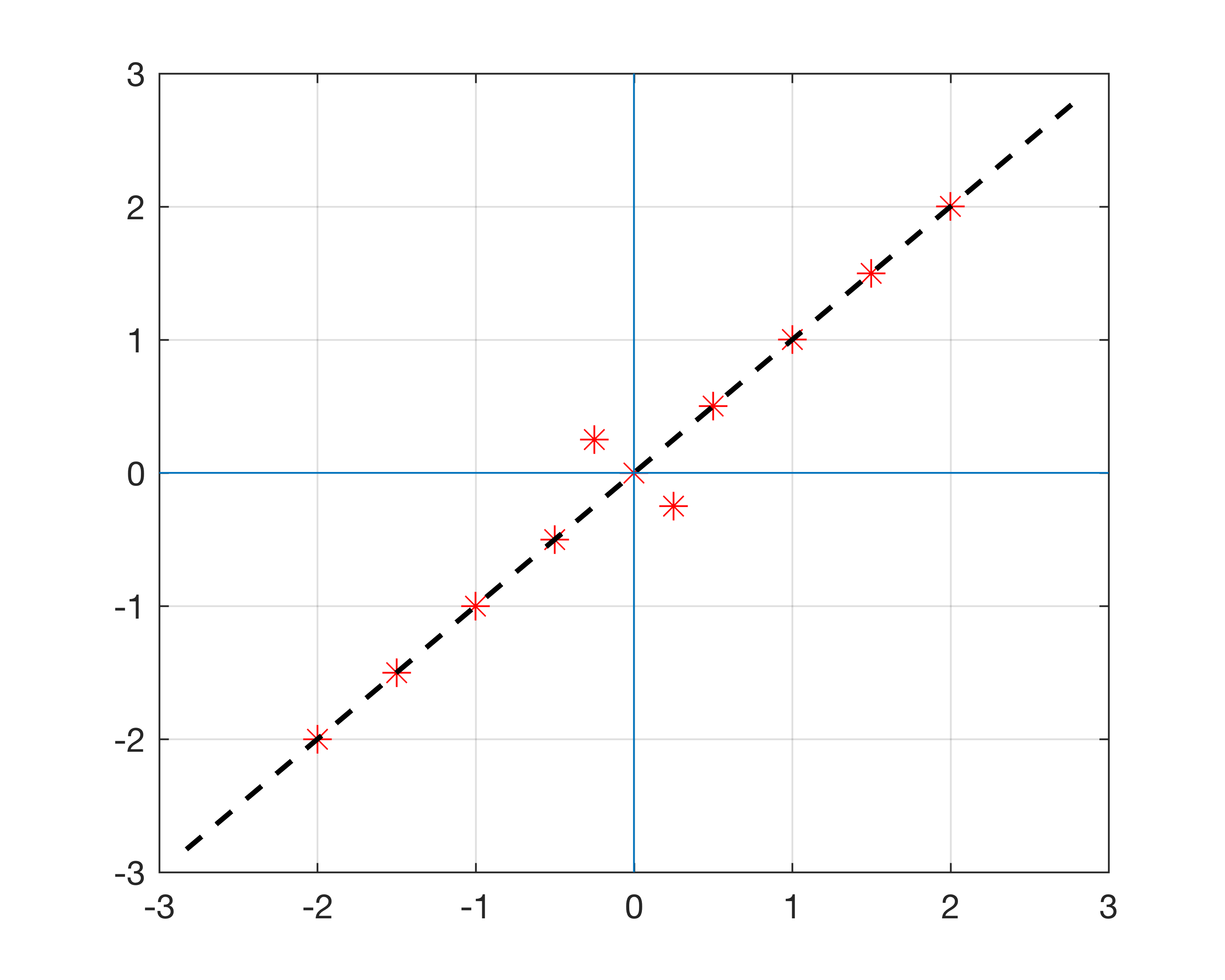
To more quantitatively understand the relation between the two competing objectives, we consider the sample mean and the uncorrected sample variance of the pairwise relative distances (2.6),

Recall that good preservation of the relative pairwise distances in (2.6) asks for $\mathcal{M}(p,x)$ being close to $1$ and the variance $\mathcal{V}(p,x)$ being small. In the following, we analyze $\tvar(px)$, $\mathcal{M}(p,x)$, and $\mathcal{V}(p,x)$ and their expectations for random $P\in\G_{k,d}$.

In Figure 2.2 we see a simple numerical experiment, where we first create an independent, normally distributed fixed data set $\{x_{i}\}_{i=1}^{m}$ with $x_{i}\in\mathbb{R}^{d}$ for $i=1,\dots,m$ and $m=100$, $d=50$. We then compute PCA, for $k=10,20,30,40$, as well as $n=10000$ random projections $p$ distributed according to $\lambda_{k,50}$. In Figure 2.2 (a) - (d) we can see that the more $k$ differs from $d$, the more PCA and random projections differ concerning $\tvar(px)$ and $\mathcal{M}(p,x)$. Those differences may lead diverse behavior in subsequent data analysis. Moreover, we compare $\mathcal{M}(p,x)$ and $\mathcal{V}(p,x)$ in Figure 2.2 (e) - (h) for the different $k$. We can see that again when $k$ is much smaller than $d$, random projections and PCA differ more concerning the variance of pairwise distances $\mathcal{V}(p,x)$. For $k=10$ the variance for PCA is higher in comparison to random projections, see Figure 2.2 (e), for $k=40$ vice versa, see Figure 2.2 (h). Note that the theoretical bounds stated in Theorem 2.1 are much higher than the dimensions $k$ used in the experiments, but the projections still preserve relative pairwise distances very well. In [7] similar observations were made on empiric experiments with image and text data.

The amount of variance kept in the principal components comparing real world and random data has been experimentally studied, e.g. in [31] and [48]. Both studies determine that the difference occurs mainly in the first principal component.

Information of data can be quantified and expressed in different ways. One crucial part in dimension reduction is the decision of what kind of information shall be kept, which depends on several parameters including the quality of the data and the analysis task. Variants of PCA, focusing on the preservation of variance, have been widely used in real world problems with big success, especially in denoising, when the preservation of all pairwise relative distances may be counterproductive, e.g. in dMRI imaging [53] and color filter array images [57]. Drawbacks are the necessity for all data being available from the start and the high computational costs. For very high dimensional and large data sets the computation of PCA is often not feasible. Besides the huge benefit of data independence and low computational cost when using random projections, the near-isometry property often allows to establish that the solution found in the low-dimensional space is a good approximation to the solution in the original space ([1], [37]).

Algorithms in machine learning often need or benefit from sufficient estimates of pairwise distances, e.g. approximate nearest-neighbor problems, supervised classification [29] and subspace clustering [28]. In [35] algorithmic applications of near-isometry embeddings have been introduced. In [7] random projections have been successfully applied to noisy and noiseless text and image data. The experimental studies include the comparison of preservation of pairwise distances between random projections and PCA. The results coincide with our observations, that for $k>d/2$ PCA is able to preserve the pairwise distances sufficiently, whereas for $k<d/2$ PCA distorts them. The smaller $k$ the worse the distortion, whereas random projections preserve similarities still well for very small $k$, while being computationally much cheaper than PCA. One should point out again that favoring preservation of pairwise distances relies on the accuracy of the original distances.

PCA and random projections are orthogonal projections favoring two different aims. We want to study in the context of the whole set of orthogonal projections if the two objectives O1) and O2) could be reached at the same time. We will see that the objectives act competing and therefore we suggest a balancing projector for tasks that benefit from both objectives.

For further mathematical analysis we first introduce a more general class of probability measures on $\G_{k,d}$ that resemble $\lambda_{k,d}$ sufficiently well:

Existence of cubature measures is studied, for instance, in [16]. For random $P$, we now determine the expectation values for our $3$ quantities of interest: $\tvar(Px)$, $\mathcal{M}(P,x)$, and $\mathcal{V}(P,x)$. If $P\sim\lambda$ and $\lambda$ is a cubature measure of strength at least $2$, the identities (A.2) and (A.3) in the appendix and a short calculation yield

where $a_{k,d}=\tfrac{2d(d-k)}{k(d-1)(d+2)}$. The expected sample variance in (2.12) satisfies

This asymptotic bound relates to Theorem 2.2 and alludes to a near-isometry property of the type (2.7) for $k$ sufficiently large.

The following Theorem 2.5 provides a lower bound for random $P$ on the population correlation

It holds for arbitrary dimensions $d$ and subsequently specifies the asymptotic behavior for $d\rightarrow\infty$:

The strong correlation for large dimensions $d$ in the second part of Theorem 2.5 suggests that increasing $\tvar(Px)$ may also lead to increasing $\mathcal{M}(P,x)$, see Figure 2.3 for illustration. Thus, large projected total variance $\tvar(Px)$ and the preservation of scaled pairwise distances, i.e. $\mathcal{M}(P,x)$ being close to $1$, are competing properties. As discussed in Section 2.3, the choice of which kind of information is favorable to preserve, depends on the data and the task; e.g. denoising (O1) and nearest neighbor classification (O2). PCA and random projections are extreme in preserving either O1) or O2). We will heuristically study the behavior of orthogonal projections balancing both objectives in the next section and will state a numerical experiment where a balancing projector yields highest classification accuracy.

Let the covering radius of a set $\{p_{l}\}_{l=1}^{n}\subset\G_{k,d}$ be denoted by

where $\|\cdot\|_{\F}$ is the Frobenius norm. The smaller the covering radius, the better the set $\{p_{l}\}_{l=1}^{n}$ represents the entire space $\G_{k,d}$. I.e., there are smaller holes and the points $\{p_{l}\}_{l=1}^{n}$ are better distributed within $\G_{k,d}$. Following Lemma 2.1 we can connect finite sets of projections and their covering radius to the near-isometry property:

The accuracy of the near-isometry property in (3.2) depends on the covering radius. Therefore, a set $\{p_{l}\}_{l=1}^{n}\in\G_{k,d}$ with a small covering radius $\varrho$ is more likely to contain a projector with better preservation of pairwise relative distances. According to [11], it holds that ¹¹ 1 We use the symbols $\lesssim$ and $\gtrsim$ to indicate that the corresponding inequalities hold up to a positive constant factor on the respective right-hand side. The notation $\asymp$ means that both relations $\lesssim$ and $\gtrsim$ hold. $\varrho\gtrsim n^{-\frac{1}{k(d-k)}}$, and we shall see next, how to achieve this lower bound.

A set of projectors $\{p_{l}\}_{l=1}^{n}\subset\G_{k,d}$ is called a $t$-design if the associated normalized atomic measure $\frac{1}{n}\sum_{l=1}^{n}\delta_{p_{l}}$ is a cubature measure of strength $t$ (see Definition 2.4), see [46] for general existence results. Any sequence of $t_{i}$-designs $\{p^{i}_{l}\}_{l=1}^{n_{i}}\subset\G_{k,d}$ with $t_{i}\rightarrow\infty$ satisfies

and moreover, the bound $n_{i}\gtrsim t_{i}^{k(d-k)}$ holds, cf. [16, 11]. To relate $n_{i}$ with $\varrho_{i}$ via $t_{i}$, a sequence of $t_{i}$-designs $\{p^{i}_{l}\}_{l=1}^{n_{i}}\subset\G_{k,d}$ is called a low-cardinality design sequence if $t_{i}\rightarrow\infty$ and

For their existence and numerical constructions, we refer to [22] and [10, 11]. According to [11], see also (3.3) and (3.4), any low-cardinality design sequence $\{p^{i}_{l}\}_{l=1}^{n_{i}}$ covers asymptotically optimal, i.e.,

Benefiting from the covering property, we will use low-cardinality design sequences as a representation of the overall space of orthogonal projectors $\G_{k,d}$.

With the linear least squares fit we can directly gain information about the relation between $\mathcal{M}(p,x)$ and $\tvar(px)$ for a given data set $x=\{x_{i}\}_{i=1}^{m}\subset\mathbb{R}^{d}$ when $p$ varies. Given the two samples

the linear least squares fitting provides the best fitting straight line,

where $s$ and $\gamma$ are determined by the sample variances and the sample covariance. If $\{p_{l}\}_{l=1}^{n}$ is a $2$-design, then the sample (co)variances coincide with the respective population (co)variances for $P\sim\lambda_{k,d}$, see Appendix A.3 for further details. It follows that

The quantities $s$ and $\gamma$ can be directly computed, where $\tvar(x)$ is given by (2.2) and the covariances are stated in Corollary A.1. Note that (3.6) and (3.7) are now independent of the particular choice of $\{p_{l}\}_{l=1}^{n}$.

The correlation between the two samples (3.5) yields additional information about their relation. As before, if $\{p_{l}\}_{l=1}^{n}$ is a $2$-design, then the sample correlation coincides with the population correlation (2.13) for $P\sim\lambda_{k,d}$, cf. Appendix A.3. High correlation for a specific data set $x$ suggests that random projections and PCA preserve competing properties, whose benefits need to be assessed for the specific subsequent task.

In the experiment we use projections $p\in\G_{2,4}$ reducing the original dimension from $d=4$ to $k=2$. As a finite representation of the overall space, we use a t-design of strength $14$ from a low-cardinality sequence (see Section 3.1) consisting of $8475$ orthogonal projectors. Note that the dimension reduction in practice takes place by applying $q\in\mathcal{V}_{k,d}$ with $q^{\top}q=p\in\G_{k,d}$, where

denotes the Stiefel manifold. When taking norms, $p$ and $q$ are interchangeable, i.e., $\|q(x)\|^{2}=\|p(x)\|^{2}$, for all $x\in\mathbb{R}^{d}$. Therefore we can use w.l.o.g. the theory developed for $p$.

The projections are chosen in a deterministic manner viewing the previously described competing properties. In Figure 4.1 the three quantities $\tvar(px)$, $\mathcal{M}(p,x)$ and $\mathcal{V}(p,x)$ are pairwise plotted for all projectors in $\{p_{l}\}_{l=1}^{8475}$. For comparison we choose the following projections $p\in\{p_{l}\}_{l=1}^{8475}\subset\G_{2,4}$, see Figure 4.1(a) for a visualization.

• $p_{\times}$

  closest to the expected values $1$ and $\tfrac{k}{d}\tvar(x)$ (see (2.10) and (2.11)),

• $p_{\Diamond}$

  preserving $\mathcal{M}(p,x)\approx 1$ and maximizing $\tvar(px)$,

• $p_{\text{\scalebox{0.8}{$\square$}}}$

  preserving $\mathcal{M}(p,x)\approx 1$ and minimizing $\tvar(px)$,

• $p_{\text{\scalebox{0.6}{$\bigcirc$}}}$

  $\tvar(px)\approx\tvar(p_{\Diamond}x)$ and maximizing $\mathcal{M}(p,x)$,

• $p_{\Huge\star}$

  minimal $\tvar(px)$,

• $p_{*}$

  maximal $\tvar(px)$ (PCA).

In Figure 4.1(b) we see the linear least squares fitting line, computed directly and via the slope and intercept as stated in (3.6) and (3.7). The correlation coefficient (2.13) is $0.98$, which suggests that preserving the two properties is highly competing and needs to be balanced.

In Table 4.1 the classification results of the iris data are presented. We can see that in this comparison the projector $p_{\Diamond}$, which corresponds to preserving $\mathcal{M}(p,x)\approx 1$ and maximizing $\tvar(px)$, yields the highest and most robust results. It even yields better results than working with the original input data. The projections that preserve $\mathcal{M}(p,x)\approx 1$ but do not take care of the magnitude of the total variance yield much worse results. On the other hand, the projections that just focus on high total variance still do not yield as high results as the projection $p_{\Diamond}$ that balances both properties.

Let the training data be input vectors $\{x_{i}\}_{i=1}^{m}\subset\mathbb{R}^{r}$ with associated target values $\{y_{i}\}_{i=1}^{m}\subset\mathbb{R}^{s}$. We consider training a neural network

where $\theta\in\mathbb{R}^{N}$ corresponds to the vector of all free parameters of a fixed architecture. In each optimization step for $\theta$, the network’s output $\{\hat{y}_{i}=f_{\theta}(x_{i})\}_{i=1}^{m}\subset\mathbb{R}^{s}$ is compared with the targets $\{y_{i}\}_{i=1}^{m}$ via an underlying loss function $L$.

In contrast to ordinary learning problems with highly accurate target data, complicated learning tasks arising in many real world problems do not yield sufficient results when optimizing neural networks with standard loss functions $L$, such as the widely used mean least squares error

The training data may include important information that is obvious for humans, but poorly represented within the original target data and therefore lacks consideration in the learning process. To overcome this issue, we propose to add information tailored to the particular learning problem represented by additional features of the outputs and targets.

First, we select transformations

to enable error estimation in transformed output/target spaces. Note that the transformations $T_{j}$ are not required to be linear. However, they should be piecewise differentiable to enable subsequent optimization of the loss function with gradient methods. We shall allow for additional weighting of the transformations $T_{1},\dots,T_{d}$ to facilitate the selection of features for a specific learning problem. The previous sections suggest that orthogonal projections can provide favorable feature combinations, which essentially turns into a weighting procedure.

To enable suitable projections, we stack the $d$ output/target features

so that applying a projector $p\in\G_{k,d}$ to each column of $T(y_{i})$ yields $p(T(y_{i}))\in\mathbb{R}^{d\times t}$. We now define the augmented target loss function with projections by

where $\alpha>0$ and $L$, $\tilde{L}$ correspond to conventional loss functions. Apparently, $L_{p}$ depends on the choice of $p\in\G_{k,d}$. The projection $p(T(y_{i}))$ weighs the previously chosen feature transformations $T(y_{i})$. Standard choices of $L$ and $\tilde{L}$ are $L_{\MSE}$, in which case $L_{p}$ becomes

It should be mentioned that $\alpha$ resembles a regularization parameter. The actual minimization of (5.1) among $\theta$ is usually performed through Tikhonov type regularization in many standard deep neural network implementations. The formulation (5.2) adds one further variational step for beneficial output data representation.

For the projected feature transformations in the augmented target loss function it is not possible to identify a balancing projection $p$ heuristically (such as $p_{\Diamond}$ in Section 4), because the output $y$ changes in each iteration when the loss function is called. In the following clinical numerical experiment we overcome this issue by using random projections and PCA in each optimization step and compare it to prior deterministic choices of projections.

In this application, OCT images of different retinal diseases (diabetic macular edema and retinal vein occlusion) were provided by the Vienna Reading Center recorded with the Spectralis OCT device (Heidelberg Engineering, Heidelberg, Germany). Each patient’s OCT volume consists of $49$ cross-sections/slices ($496\times 512$ pixels) recorded in an area of $6\times 6$ mm in the center of the human retina, which is the part of the retina responsible for vision. Each of the slices was manually annotated by a trained grader of the reading center. This is a challenging and time-consuming procedure that is not feasible in clinical routine but only in a research setting. The binary pixelwise annotations serve as target values, enabling a supervised learning framework.

The objective is to accurately detect the photoreceptor layers and their disruptions pixelwise in each OCT slice by training a deep convolutional neural network with a suitable loss function. The learning problem is complicated by potentially inaccurate target annotations, as studies have shown that inconsistencies between trained graders are common, cf. [52]. Moreover, the learning task is unbalanced in the sense that there are many more slices showing none or very little disruptions. We shall observe that optimization with respect to standard loss functions performs poorly in regards to detecting disruptions. The augmented target loss function proposed in the previous section can enhance the detection.

We implemented our experiments using Python 3.6 with Pytorch 1.0.0. A deep convolutional neural network $f_{\theta}$ is trained by applying the U-Net architecture reported in [45] with a sigmoid activation function and Tikhonov regularization. A set of $20$ OCT volumes ($980$ slices) from different patients with corresponding annotations are used for training, where $4$ volumes were used for calibration (validation set). Another $2$ independent test volumes were identified for evaluating the results, one without any disruptions in the photoreceptor layers, whereas the other one includes a high number of disruptions.

Each OCT slice is represented by a vector $x_{i}\in\mathbb{R}^{r}$ with $r=496\cdot 512$. The collection $\{x_{i}\}_{i=1}^{m}$ corresponds to all slices from the training volumes, i.e. $m=20\cdot 49$. Further matching the notation of the previous section, we have $r=s$ and $f_{\theta}:\mathbb{R}^{r}\rightarrow\mathbb{R}^{r}$ with binary target vectors $y_{i}\in\{0,1\}^{r}$. We observe that disruptions are not identified reliably when using the least squared loss function (5.1). To overcome this issues, we use the proposed augmented target loss function with least squared losses as stated in (5.3).

To enhance disruptions within the output/target space, we heuristically choose $d=4$ local features of the original representation. They are derived from convolutions with $2$ edge filters, $T_{1}$ (Prewitt) and $T_{2}$ (Laplacian of Gaussian), and from $2$ Gaussian highpass filters, yielding $T_{3}$ and $T_{4}$. Note that these feature transformations keep the same size, i.e. $T_{j}:\mathbb{R}^{r}\rightarrow\mathbb{R}^{r}$ for $j=1,\ldots,d$. See Figure 6.2 for example images.

We can derive several augmented target loss functions $L_{p}$ by choosing different $p\in\G_{k,d}$ for (5.2). In this experiment we use the following projections:

• •

  $p=I_{4}$,

• •

  $\{p_{l}\}_{l=1}^{15}$, all projections from a t-design of strength $2$ $\subset\G_{2,4}$ (see [10]),

• •

  $p_{\PCA}\in\G_{2,4}$, projection determined by PCA on the training data,

• •

  $p_{\lambda_{2,4}}$, random projection chosen according to $\lambda_{2,4}$ in each mini-batch.

Since the detection problem is highly unbalanced we use precision/recall curves [15] for evaluating the overall performance of each loss function model. The area under the curve (AUC) was used as a numerical indicator of the success rate, [43]. The higher the AUC the better the classification.

The results of the different loss functions on the independent test set are stated in Table 6.1. Due to the imbalance within the data, the photoreceptor region is identified well, but disruptions are not identified reliably when using the least squared loss function (5.1). For $\alpha=0.1$ all proposed augmented target loss functions $L_{p}$ clearly increase the success rate of the disruption quantification. Note that all projections are independent from the actual data set, except PCA that was computed beforehand on the training data.

The features itself (i.e. $p=I_{4}$) improve the quantification and weighting them by projections increases the results even more: using the fixed projection $p_{12}$ from the t-design sequence $\{p_{l}\}_{l=1}^{15}$ on the output/target features yields the highest accuracy for photoreceptors and disruptions. This corresponds to the results of the previous sections, stating that depending on the particular data there are projections in the overall space acting beneficially.

Since this projection generally cannot be found beforehand, using random projections in each loss function evaluation step is easier possible in practice and independent from the data. They can be computed very efficiently and randomization can generalize and robusten the information, cf. [37]. In the following we will view a second classification problem based on spectrograms, where augmented target loss functions with random projections can improve the accuracy.

The publicly available GoodSounds dataset [44] contains recordings of single notes and scales played by several single instruments. To gain equally balanced input classes we restrict the classification problem to $6$ instruments: clarinet, flute, trumpet, violin, alto saxophone and cello. Note that the recordings are monophonic, so that each recording yields one spectrogram that we aim to correctly assign to one of the $6$ instruments.

After removing the silence [3, 40], segments from the raw audio files are transformed into log mel spectrograms [20], so that we obtain images of time-frequency representations with size $100\times 100$. One example spectrogram for each class of instruments is depicted in Figure 7.1.

We implemented a fully convolutional neural network $f_{\theta}:\mathbb{R}^{r}\to[0,1]^{s}$, cf. [36], where $r=100\times 100$ and $s=6$, in Python 3.6 using Keras 2.2.4 framework [21] and trained it on the Nvidia GTX 1080 Ti GPU. The data is split into $140\,722$ training, $36\,000$ validation and $36\,000$ independent test samples. We heuristically choose $d=16$ output features arising directly from the particular output class. The transformations $T_{1},\dots,T_{16}$, with $T_{j}:\mathbb{R}^{6}\to\mathbb{R}$ for $j=1,\dots,16$, are then given by the inner product of the output/target and the feature vectors. Amongst others the features are chosen from the enhanced scheme of taxonomy [55] and from the table of frequencies, harmonics and under tones [59]. We use the proposed augmented target loss function $L_{p}$ (5.2), where $L_{1}$ corresponds to the categorical-cross-entropy loss [58] and $L_{2}$ to the mean squared error as in (5.3). We consider here two choices of $p$: the identity $I_{16}$ and random projectors $p\sim\lambda_{6,16}$ in $\G_{6,16}$.

The deep learning model is sensitive to various hyper-parameters, including $\alpha$ and $p$, in addition to conventional parameters, such as the number of convolutional kernels, learning rate and the parameter $\beta$ for Tikhonov regularization. To find the best choices in a fair trial we utilize a random hyper-parameter search approach, where we train $60$ models and select the $3$ best ones for a more precise search over different $\alpha$ in the augmented target loss function and $\beta$ for Tikhonov regularization. This results in $212$ models that are evaluated on the training and validation set. Finally, we select the best model based on the accuracy of the validation set and evaluate it on the independent test set. For comparison we also evaluate this model with no Tikhonov regularization, i.e. $\beta=0$, see Table 7.1.

Table 7.1 shows that no regularization and no features provide the poorest results. It seems that adding features with random projections have a regularizing effect and improve the results significantly. As expected, it is important to include Tikhonov regularization on $\theta$. Further enhancement happens by adding features via the modified augmented target loss function with or without additional weighting from projections. All results are very stable and are generalizing very well from training to the independent test set, see [27] for further details.

References

- [1] D. Achlioptas, Database-friendly random projections: Johnson-Lindenstrauss with binary coins, Journal of Computer and System Sciences 66 (2003), no. 4, 671–687.
- [2] C. Bachoc and M. Ehler, Tight -fusion frames, Appl. Comput. Harmon. Anal. 35 (2013), no. 1, 1–15.
- [3] C. Bagwell, SoX - Sound Exchange the swiss army knife of sound processing., https://launchpad.net/ubuntu/+source/sox/14.4.1-5, Accessed: 2018-10-31.
- [4] K. Ball, An elemntary introduction to modern convex geometry, Flavors in Geometry 31 (1997), 1–58.
- [5] R. Baraniuk, M. Davenport, R. DeVore, and M. Wakin, A simple proof of the restricted isometry property for random matrices, Constr. Approx. 28 (2008), no. 3, 253–263.
- [6] R. G. Baraniuk and M. B. Wakin, Random projections of smooth manifolds, Foundations of Computational Mathematics, vol. 9, 2006, pp. 941–944.
- [7] Ella Bingham and Heikki Mannila, Random projection in dimensionality reduction: Applications to image and text data, Proceedings of the Seventh ACM SIGKDD International Conference on Knowledge Discovery and Data Mining (New York, NY, USA), KDD ’01, ACM, 2001, pp. 245–250.
- [8] B. Bodman, M. Ehler, and M. Gräf, From low to high-dimensional moments without magic, J. Theor. Probab. (2017).
- [9] A. Breger, M. Ehler, H. Bogunovic, S. M. Waldstein, A. Philip, U. Schmidt-Erfurth, and B. S. Gerendas, Supervised learning and dimension reduction techniques for quantification of retinal fluid in optical coherence tomography images, Eye, Springer Nature (2017).
- [10] A. Breger, M. Ehler, and M. Gräf, Quasi Monte Carlo integration and kernel-based function approximation on Grassmannians, Frames and Other Bases in Abstract and Function Spaces, Applied and Numerical Harmonic Analysis series (ANHA), Birkhauser/Springer (2017).
- [11] A. Breger, M. Ehler, and M. Gräf, Points on manifolds with asymptotically optimal covering radius, Journal of Complexity 48 (2018), 1–14.
- [12] E. J. Candès and T. Tao, Decoding by linear programming, IEEE Trans. Inform. Theory 51 (2005), no. 12, 4203–4215.
- [13] R. Caruana, Multitask learning, Machine Learning 28 (1997), no. 1, 41–75.
- [14] S. Dasgupta and A. Gupta, An elementary proof of a theorem of Johnson and Lindenstrauss, Random Structures & Algorithms 22 (2003), no. 1, 60–65.
- [15] J. Davis and M. Goadrich, The relationship between precision-recall and roc curves, Proceedings of the 23rd International Conference on Machine Learning (New York, NY, USA), ICML ’06, ACM, 2006, pp. 233–240.
- [16] P. de la Harpe and C. Pache, Cubature formulas, geometrical designs, reproducing kernels, and Markov operators, Infinite groups: geometric, combinatorial and dynamical aspects (Basel), vol. 248, Birkhäuser, 2005, pp. 219–267.
- [17] M. Dörfler, R. Bammer, and T. Grill, Inside the spectrogram: Convolutional neural networks in audio processing, IEEE International Conference on Sampling Theory and Applications (SampTA) (2017), 152–155.
- [18] M. Dörfler, T. Grill, R. Bammer, and A. Flexer, Basic filters for convolutional neural networks applied to music: Training or design, Neural Comput. & Applications (2018), 1–14.
- [19] Alexey Dosovitskiy and Thomas Brox, Generating images with perceptual similarity metrics based on deep networks, Proceedings of the 30th International Conference on Neural Information Processing Systems (USA), NIPS’16, Curran Associates Inc., 2016, pp. 658–666.
- [20] B. McFee et al., Librosa: 0.6.2, https://doi.org/10.5281/zenodo.1342708, 2018.
- [21] F. Chollet et al., Keras, https://keras.io, 2015.
- [22] U. Etayo, J. Marzo, and J. Ortega-Cerdà, Asymptotically optimal designs on compact algebraic manifolds, J. Monatsh. Math. 186 (2018), no. 2, 235–248.
- [23] A.F. Frangi, W.J. Niessen, K.L. Vincken, and M.A. Viergever, Multiscale vessel enhancement filtering, Lecture Notes in Computer Science 1496 (1998).
- [24] Pierre-Antoine Ganaye, Michaël Sdika, and Hugues Benoit-Cattin, Semi-supervised learning for segmentation under semantic constraint: 21st international conference, granada, spain, september 16-20, 2018, proceedings, part iii, pp. 595–602, 09 2018.
- [25] B.S. Gerendas, X. Hu, A. Kaider, A. Montuoro, A. Sadeghipour, S.M. Waldstein, and U. Schmidt-Erfurth, Oct biomarkers predictive for visual acuity in patients with diabetic macular edema, Investigative Ophthalmology & Visual Science 58 (2017), no. 8, 2026–2026.
- [26] G. H. Golub and C. F. Van Loan, Matrix computations, Johns Hopkins Studies in the Mathematical Sciences, The Johns Hopkins University Press, 1996.
- [27] P. Harar, Orthovar, https://gitlab.com/hararticles/orthovar, 2018.
- [28] Reinhard Heckel, Michael Tschannen, and Helmut Bölcskei, Dimensionality-reduced subspace clustering, Information and Inference: A Journal of the IMA 6 (2017).
- [29] C. Hedge, A. C. Sankaranarayanan, W. Yin, and R. G. Baraniuk, Numax: A convex approach for learning near-isometric linear embeddings, IEEE Transactions on Signal Processing 83 (2015).
- [30] Justin Johnson, Alexandre Alahi, and Li Fei-Fei, Perceptual losses for real-time style transfer and super-resolution, ECCV, 2016.
- [31] J. R. Karr and T. E. Martin, Random numbers and principal components: further searches for the unicorn, Tech. report, United States Forest Service General Technical Report, 1981.
- [32] F. Krahmer and R. Ward, New and improved Johnson Lindenstrauss embeddings via the restricted isometry property, SIAM Journal on Mathematical Analysis 43 (2011), no. 3, 1269–1281.
- [33] G. Kutyniok, W.-Q. Lim, and R. Reisenhofer, Shearlab 3d: Faithful digital shearlet transforms based on compactly supported shearlets, ACM Trans. Math. Softw. 42 (2016, www.shearlab.org).
- [34] Christian Ledig, Lucas Theis, Ferenc Huszar, Jose Caballero, Andrew P. Aitken, Alykhan Tejani, Johannes Totz, Zehan Wang, and Wenzhe Shi, Photo-realistic single image super-resolution using a generative adversarial network, 2017 IEEE Conference on Computer Vision and Pattern Recognition (CVPR) (2017), 105–114.
- [35] Nathan Linial, Eran London, and Yuri Rabinovich, The geometry of graphs and some of its algorithmic applications, Combinatorica 15 (1995), no. 2, 215–245.
- [36] J. Long, E. Shelhamer, and T. Darrell, Fully convolutional networks for semantic segmentation, Proceedings of the IEEE conference on computer vision and pattern recognition, 2015, pp. 3431–3440.
- [37] Michael W. Mahoney, Randomized algorithms for matrices and data, Foundations and Trends® in Machine Learning 3 (2011), no. 2, 123–224.
- [38] J. Matousek, On variants of the Johnson-Lindenstrauss lemma, Random Structures & Algorithms 33 (2008), no. 2, 142–156.
- [39] B. Moore, Principal component analysis in linear systems: Controllability, observability, and model reduction, IEEE Transactions on Automatic Control 26 (1981).
- [40] J. Navarrete, The sox of silence, https://digitalcardboard.com/blog/2009/08/25/the-sox-of-silence, 2009.
- [41] S. Neumayer, M. Nimmer, S. Setzer, and G. Steidl, On the robust PCA and Weiszfeld’s algorithm, Appl. Math. Optim. (2019).
- [42] Ozan Oktay, Enzo Ferrante, Konstantinos Kamnitsas, Mattias Heinrich, Wenjia Bai, Jose Caballero, Ricardo Guerrero, Stuart A Cook, Antonio de Marvao, Timothy Dawes, Declan O’Regan, Bernhard Kainz, Ben Glocker, and Daniel Rueckert, Anatomically constrained neural networks (acnn): Application to cardiac image enhancement and segmentation, IEEE Transactions on Medical Imaging PP (2017).
- [43] G. Pabst, Parameters for compartment-free pharmacokinetics - standardisation of study design, data analysis and reporting, ch. 5. Area under the concentration-time curve, pp. 65–80, Shaker Verlag, 1999.
- [44] O. Romani Picas, H. Parra Rodriguez, D.Dabiri, H.Tokuda, W. Hariya, K. Oishi, and X. Serra, A real-time system for measuring sound goodness in instrumental sounds, Audio Engineering Society Convention 138, Audio Engineering Society, 2015.
- [45] O. Ronneberger, P. Fischer, and T. Brox, U-net: Convolutional networks for biomedical image segmentation, arxive:1505.04597 (2015).
- [46] P. Seymour and T. Zaslavsky, Averaging sets: a generalization of mean values and spherical designs, Advances in Math. 52 (1984), 213–240.
- [47] Karen Simonyan and Andrew Zisserman, Very deep convolutional networks for large-scale image recognition, arXiv 1409.1556 (2014).
- [48] Dean F. Stauffer, Edward O. Garton, and R. Kirk Steinhorst, A comparison of principal components from real and random data, Ecology 66 (1985), no. 6, 1693–1698.
- [49] Russell Stewart and Stefano Ermon, Label-free supervision of neural networks with physics and domain knowledge, AAAI, 2017.
- [50] Gian-Andrea Thanei, Christina Heinze, and Nicolai Meinshausen, Random projections for large-scale regression, pp. 51–68, Springer International Publishing, Cham, 2017.
- [51] M. Udell, Generalized low rank models, Ph.D. thesis, Stanford University, 2015.
- [52] E. S. Varnousfaderani, J. Wu, W.-D. Vogl, A.-M. Philip, A. Montuoro, R. Leitner, C. Simader, S. M. Waldstein, B. S. Gerendas, and U. Schmidt-Erfurth, A novel benchmark model for intelligent annotation of spectral-domain optical coherence tomography scans using the example of cyst annotation, Computer Methods and Programs in Biomedicine 130 (2016), 93–105.
- [53] Jelle Veraart, Dmitry S. Novikov, Daan Christiaens, Benjamin Ades-aron, Jan Sijbers, and Els Fieremans, Denoising of diffusion mri using random matrix theory, NeuroImage 142 (2016), 394 – 406.
- [54] R. Vershynin, Introduction to the non-asymptotic analysis of random matrices, Compressed sensing, Theory and Applications (Y. Eldar and G. Kutyniok, eds.), Cambridge University Press, 2012, pp. 210–268.
- [55] E.M. von Hornbostel and C. Sachs, Classification of musical instruments: Translated from the original german by anthony baines and klaus p. wachsmann, The Galpin Society Journal (1961), 3–29.
- [56] Jason Yosinski, Jeff Clune, Yoshua Bengio, and Hod Lipson, How transferable are features in deep neural networks?, Proceedings of the 27th International Conference on Neural Information Processing Systems - Volume 2 (Cambridge, MA, USA), NIPS’14, MIT Press, 2014, pp. 3320–3328.
- [57] L. Zhang, R. Lukac, X. Wu, and D. Zhang, Pca-based spatially adaptive denoising of cfa images for single-sensor digital cameras, IEEE Transactions on Image Processing 18 (2009), no. 4, 797–812.
- [58] Z. Zhang and M. Sabuncu, Generalized cross entropy loss for training deep neural networks with noisy labels, Advances in Neural Information Processing Systems (NIPS) 31 (2018).
- [59] Inc. ZyTrax, Frequency ranges, http://www.zytrax.com/tech/audio/audio.html, 2018.