Classical General Relativity Effects to Second Order in Mass, Spin, and Quadrupole Moment
Abstract
In this contribution, we calculate the light deflection, perihelion shift, time delay and gravitational redshift using an approximate metric that contains the Kerr metric and an approximation of the Erez-Rosen spacetime. The results were obtained directly using Mathematica [20]. The results agree with the ones presented in the literature, but they are extended until second order terms of mass, angular momentum and mass quadrupole. The inclusion of the mass quadrupole is done by means of the metric; no expansion of the gravitational potential as in the parameterized post-Newtonian is required.
1 Introduction
Einstein’s General Theory of Relativity is a metric theory of gravity that relates the mass-energy content of the universe with the space-time curvature through the Einstein field equations:
| (1) |
where the right-hand side of this equation depends on the stress-energy tensor which describes the mass-energy sources of gravitational fields, and the left-hand side depends on the metric elements which describe the space-time curvature. are the Ricci tensor components, is the scalar curvature, and is the cosmological constant. In this article, the geometrical units are employed, so that . The cosmological constant is set .
In 1916, Karl Schwarzschild discovered a solution to the Einstein field equations in vacuum, suitable for describing the spacetime in the empty space surrounding a spherical, static object [32]. Ever since then, this metric has been used to describe a wide range of phenomena, including light deflection close to a massive star, planetary precession of the perihelion, time delay and gravitational redshifts for weak fields. G. Erez and N. Rosen introduced the effects of mass quadrupole as exact solution in 1959 [3, 9]. This derivation had some errors which were corrected by Doroshkevich et al. [7], Winicour et al. [36] and Young and Coulter [37]. The exact solution for a rotating black hole (BH) could only be solved as late as 1963 by Roy P. Kerr [14]. There are exact solutions containing the Erez-Rosen and Kerr features, such spacetimes are cumbersome. A new approximate metric representing the spacetime of a rotating deformed body is obtained by perturbing the Kerr metric to include up to the second order of the quadrupole moment [11]. This kind of approximations is valid because the quadrupole moment is small generally for a variety of astrophysical objects. Observing the Spin of rotating BH is possible by measuring the orbital angular momentum of light propagating around it, as well as BH shadow circularity analysis [33].
In the literature, calculations that include the mass quadrupole are only done using (parameterized) post Newtonian metrics. To introduce the mass quadrupole, the gravitational potential is expressed as a multipolar expansion [19, 23, 25, 26, 27, 28, 29]. In our calculation we perform no such expansion of the gravitational potential. The quadrupole parameter is introduced from the metric.
Now, it is possible to do such calculation in a straightforward manner using software like Mathematica. In this contribution, we present the results of light deflection, perihelion shift, time delay and gravitational redshift using this software. The results were compared with the ones obtained from the Reduce software.
This paper is organized as follows. The classical tests of general relativity are described in section 2. The parameterized post-Newtonian formalism is introduced in section 3. The approximate metric with three parameters () is described in section 4. The metric potentials are expanded in a Taylor series up to second order of , and . The resulting metric is transformed into a Hartle-Thorne form. In section 6 we calculate the angle of the deflection of light in traveling in the equatorial plane of our metric. In section 7, we present the necessary calculations to obtain the angle of Precession of the perihelion of the orbit of a planet in the presence of a space-time described by our metric. In section 8, we calculate the time delay of light traveling between two points and in section 9, the expression for the gravitational redshift in two different positions in our space-time is obtained. The Mathematica notebook is available upon request. Our concluding remarks are presented in the last section.
2 The Classical Tests
In the solar system, most of the Newtonian mechanics predictions are in good agreement with observations. However, there are a few situations where general relativity (GR) is positioned as a more precise theory. Traditionally, they are Mercury’s perihelion precession, the light deflection by the Sun, the gravitational redshift of light and the time delay of light.
Mercury’s perihelion precession is the first classical test and was first noted by Le Verrier in 1859. In this phenomenon, classical contributions such as the planetary perturbations influence [17, 18], yet it remains a discrepancy of per century. The contributions from GR reports a value of per century. During the 1960’s and 1970’s there was a considerable controversy on the importance of the contribution of the solar oblateness mass quadrupole on the perihelion precession. This discussion has relaxed as the value of the solar quadrupole has been inferred to be small, on the order of [35, 18]. Using this value, it has been estimated that the contribution to the precession from the solar oblateness is of per century. Yet, its importance can not be specified until a reliable value of the quadrupole is known. The second test, the light deflection due to the massive body of the Sun, was famously first observed during the Eddington’s expedition in 1919 with a high degree of inaccuracy, but it was not observed with precision until the 70’s using radio wave interferometry. By this time, it was reported that the mean gravitational deflection was times the value predicted by GR [18]. The deflection caused by the solar oblateness can be treated as a small correction. Typically, it could modify the path of ray of light in arcseconds. Other physical property that influences light deflection is the Sun’s angular momentum, as it has been calculated that the Sun’s amount of can be responsible for a deflection of arcseconds [8].
The third test, the gravitational redshift, measures the wavelenght shift between two identical clocks placed at rest at different positions in a gravitational field. This was the first test to be proposed by Einstein, and was first tested by Pound, Rebka and Snider in the 1960s, as they measured the gamma radiation emitted by 57Fe , as they ascended or descended the Jefferson Physical Laboratory tower [18]. The fourth test, the gravitational time delay, was classified as such by Will and was first observed by Shapiro in 1964 when he discovered that a ray of light propagating in the gravitational field of a massive body will take more time traveling a given distance, than if the field were absent [18]. Gravitational time delay can be observed by measuring the round trip of a radio signal emitted from Earth and reflected from another body, such as another planet or a satellite. To properly measure the effect, it is necessary to do a differential measurement in the variations in the round trip as the target object moves through the sun’s gravitational field. This task is particularly difficult as it involves taking into account the variations in the round trip as a result of the orbital motion of the target relative to Earth [35].
Another ideal probe for testing GR is the massive black hole (MBH) located in a bright and very compact astronomical radio source called Sgr A* at the center of the Milky Way at a distance kpc and with a mass . This MBH is surrounded by the highly elliptical star S2 whose motion has been an important subject of study in the literature [38, 13]. It has been determined that S2 has a semi-major axis mas and an eccentricity , and so is possible to make an estimate of the contributions of the mass of the MBH to the orbit precession and the gravitational redshift and compare them with the values reported in the literature.
3 The Parametrized Post-Newtonian Formalism
Although it has been very successful when compared with direct observations, GR is just one of many metric theories of gravity, and all that distinguishes one metric theory from another is the particular way in which matter generates the metric. It is simple to perform a comparison between metric theories in the slow-motion and weak-field limit, since all of their results must agree with Newtonian phyisics.
The parametrized post-Newtonian (PPN) formalism is a device that allows the comparison between different theories of gravitation and experiments. It is motivated by the advent of alternative theories of gravitation other than GR during the second half of the twentieth century. It has provided a common framework to quantify deviations from GR which are small in the post-Newtonian order.
As the various theories of gravitation involve mathematical objects such as coordinates, mass variables and metric tensors, PPN formalism is provided with a set of ten parameters which describe the physical effects of these theories. The so called Eddington-Robertson-Schiff parameters and are the only non-zero parameters in GR, hence they are significant in the study of classical tests. measures whether gravitational fields do interact with each other, while quantifies the space-curvature produced by unit rest mass, and both their values is one in GR [18].
In this context, it is very important to mention Gaia, the ESA space astrometry mission launched in late 2013. Through its detectors, it will perform Eddington-like experiments through the comparison between the pattern of the starfield observed with and without Jupiter. For this purpose, it is vital to have a formula relevant for the monopole and quadrupole light deflection for an oblate planet. These results will provide a new independent determination of and evidence of the bending effect of the mass quadrupole of a planet [4, 5]. It is currently accepted that is less than .
It is also relevant to highlight the use of radiometric range measurements to the MESSENGER spacecraft in orbit around Mercury to estimate the precession of Mercury’s perihelion. Knowing a suitable relationship between this classical test and the quadrupole allows to decouple and the solar quadrupole to yield [24]. It has been conjectured that there is another additional contribution to the perihelion advance from the relativistic cross terms in the post-Newtonian equations of motion between Mercury’s interaction with the Sun and with the other planets, as well from the interaction between Mercury’s motion and the gravitomagnetic field of the moving planets. These effects are planned to be detected by the BepiColombo mission, launched in late 2018 [34].
There have been several papers that have quantified the contributions to the classical tests from various objects in the solar system. Detection and precise measurement of the quadrupolar deflection of light by objects in the solar system, at the level of a microarcsecond positional accuracy, is important as it will allow the experimental observation of a wide range of physical phenomena that will allow to test GR in a velocity and acceleration-independent-regime. There are research lines that study the effects related to the motion of planets such as the appearance of a gravitational field due to the mass dipole and methods to properly measure the quadrupole of the planets that compensate for the effects due to their movements [16]. The values shown in Table 1 illustrate the maximal magnitudes of the various gravitational effects due to the Sun and the planets at which the gravitational light deflection from that body should still be accounted for to attain a final accuracy of 1 as. Here, Second Order: PN is the post-Newtonian effect due to the spherically symmetric field of each body, Rotation accounts for the field caused by the rotational motion of the bodies, Fourth Order: PPN is the post-post Newtonian effect due to the mass, and Quadrupole: PN is the effect caused by the mass quadrupole [15].
| Stellar Object | Second Order: PN (as) | Rotation (as) | Fourth Order: PPN (as) | Quadrupole: PN (as) |
| Sun | 0.7 | 11 | 1 | |
| Mercury | - | - | - | |
| Venus | - | - | - | |
| Earth | - | - | ||
| Mars | - | - | ||
| Jupiter | 0.2 | - | ||
| Saturn | - | - | ||
| Uranus | - | - | ||
| Neptune | - | - |
Table 2 shows the values of the contributions to the gravitation delay of a radio signal as it is measured from the Earth [23].
In this formalism, the gravitational potential of an axially symmetric body can be written in the following form [12]
| (2) |
In this paper, we will consider up to second order in the PPN formalism.
| Stellar Object | Second Order: PN (ns) | Rotation (ns) | Fourth Order: PPN (ns) | Quadrupole: PN (ns) |
|---|---|---|---|---|
| Sun | ||||
| Mercury | - | |||
| Venus | - | |||
| Mars | ||||
| Jupiter | ||||
| Saturn | ||||
| Uranus | ||||
| Neptune |
4 The Metric
The metric, we will employ to do the calculations was generated in a perturbative form using the Kerr spacetime as seed metric. This approximate rotating spacetime with quadrupole moment written in standard form is as follows [10, 11]:
| (3) | |||||
where
| (4) | |||||
This spacetime has three parameters, namely mass , spin, ( as the Kerr rotation parameter) and , the mass quadrupole. It contains the Kerr and the Schwarzschild metrics. This metric is an approximation to the Erez-Rosen metric ().
According to [11], the Taylor series up to second order of and gives
| (5) | |||||
Now, in [11] a transformation was found that converts this expanded metric (4) into the expanded Hartle-Thorne (HT) metric changing that included the second order in , it is
| (6) | |||||
where
| (7) | |||||
the transformed metric components take the following form [11]
| (8) | |||||
where and . This new expanded HT form with second order quadrupole monent is a more convenient way to calculate the quantities we are going to obtain, because it is in Schwarzschild spherical coordinates.
5 The Geodesic Equation
The space-time interval between two events is defined as,
| (9) |
We can equate the interval with a proper time and so write down the following equation,
| (10) |
where is a parameter to be defined. For massive particles moving across spacetime its trajectories are described by time-like intervals (), so we set , while light trajectories are described by light-like intervals () and so we set . The former case is suitable for describing planetary motion, as its the case for planetary perihelion, while light deflection and time delay, which are light related, are described by the latter. The geodesic equations help to calculate the path with the shortest proper time between two points,
| (11) |
The geodesic equation is related to conserved quantities, as in our case when we set ,
| (12) |
We can set the conserved quantity related with the energy ,
| (13) |
When we set we obtain a conserved quantity related to the density of angular momentum along the -axis, ,
| (14) |
These relations can be reversed to obtain:
| (15) | |||||
| (16) |
| (17) |
6 Light Deflection
The effect is represented in Figure 1. We set in (10) and rearranging provides an equation for . We can use the substitution to obtain up to order :
| (18) | |||||
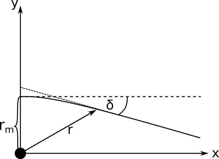
This equation can only be solved by perturbation theory. For this purpose, we propose a solution of the form
| (19) | |||||
This method brings up a number of equations of the form:
| (20) |
or,
| (21) |
and so on. For this part, we stuck to the general solutions to the differential equation as in [2],
to be
for and
for . The approximate solution is:
| (22) | |||||
The closest approach occurs when , so:
| (23) | |||||
The deflection angle can be found using the condition , that is:
| (24) | |||||
This result agrees with the result expected from the Schwarzschild metric,
up to second order in mass [2]. The evaluation of some these terms for a ray of light grazing the solar limb is presented in Table 3
| Stellar Object | First Order: Mass (as) | Rotation (as) | Second Order: Mass (as) | Quadrupole (as) |
|---|---|---|---|---|
| Sun | 7.224014 | 9.627369 | ||
| Mercury | - | |||
| Venus | - | |||
| Earth | ||||
| Mars | ||||
| Jupiter | ||||
| Saturn | ||||
| Uranus | ||||
| Neptune |
7 Precession of the Perihelion
The effect is represented in Figure 2. First, we use the geodesic equation (11) to find the conserved quantities, and the equations (15) and (16). Using these new identities, it is possible to calculate setting in (10) and imposing a planar orbit . After this, the well known variable change is used, so it is possible to find by means of:
| (25) |
After taking the second derivative with respect to , we found up to order , the result is:

| (26) | |||||
We can consider a perturbation , where is the wobble function we want to find. As such, given that , it satisfies the harmonic equation:
| (27) | |||||
It provides an angular frequency value for which . The orbit perihelion occurs when is a minimum, i.e. when the argument of the cosine function is . can be found using the condition . Although other methods can be used [6], by using the common substitution
along the Schwarzschild circular orbit approximation
this implies:
| (28) | |||||
This result agrees with the result expected from the Schwarzschild metric, , up to first order in mass. For the perihelion precession of Mercury some of the contributions can be computed as is shown in Table 4. The gravitational periastron precession in the orbit of the star S2 are also included, and they agree whit the reported value in literature of 12 arcmin per orbit ( 75 arcsec per century) near the pericentre [13].
| Body | First Order: Mass (as/cent) | Second Order: Mass (as/cent) | Quadrupole (as/cent) |
|---|---|---|---|
| S2 | 73.8075 | 0.00101207 | - |
| Mercury | 41.162 | 4.7230110-6 | 4.7230110-6 |
8 Time Delay
The effect is represented in Figure 3, as the path of rays of light are turned away from their classical trajectories. The curvature induced in the spacetime surrounding a massive body increases the travel time of light rays relative to what would be the case in flat space. Let be the maximum approach distance of a ray of light traveling near a massive body. If the beam traveled in a straight line, then . This means that

By using , it is possible to extract from , so we obtain:
| (29) | |||||
Performing an integration to go from a planet at position , to another planet at , to find the time delay:
| (30) | |||||
where , , , and .
This result agrees with the result expected from the Schwarzschild metric, up to first order in mass [21]. Some of the contributions of the gravitational delay of light grazing the solar limb and the planets as predicted by our model are presented in Table 5.
| Stellar Object | Second Order: PN (ns) | Rotation (ns) | Fourth Order: PPN (ns) | Quadrupole: PN (ns) |
|---|---|---|---|---|
| Sun | ||||
| Mercury | - | |||
| Venus | - | |||
| Mars | ||||
| Jupiter | ||||
| Saturn | ||||
| Uranus | ||||
| Neptune |
9 Gravitational Redshift
The effect is represented in Figure 4. It is possible to calculate a redshift factor by comparing the proper time for observers located at two different values of , assuming a planar orbit, .
| (31) | |||||

This result agrees with the result expected from the Schwarzschild metric, up to first order in mass [22]. The gravitational redshift in the orbit of the star S2 agrees with the reported value in literature of 103 km s-1/c near the pericentre [13, 38], as it is shown in Table 6.
| First Order: Mass (km s-1/c) | Second Order: Mass (km s-1/c) |
|---|---|
| 103.24 | 0.0532923 |
10 Conclusions
We reviewed the calculations of the classical experiments in GR with an approximative metric and taking in account all second order terms of mass, angular momentum and mass quadrupole. If we neglect these terms our results agree with the ones in the literature. By using our results, it could now be possible to estimate the value of second order terms of mass, quadrupole and angular momentum and determine how well they adapt to the predicted phenomena in the classical tests.
In PPN theory these results were obtained, but in this theory the quadrupole moment is introduced in the expansion of the mass potential. Here, this effect is introduced by the metric in a straightforward way. Our calculations were done in a simple manner using Mathematica. Moreover, we developed a Mathematica notebook, which is available upon request. The notebook is divided in sections, each one correspoding to a classical test. These calculations in the PPN method are rather complicated, but it would be interesting to expand them using the PPN methods.
As future work, it is planned to include the spin octupole and the mass hexadecapole, because now, these relativistic multipoles are currently considered in neutron stars calculations. For instance, to determine the innermost stable circular orbit or the precession frequencies, these relativistic multipole moment play an important role [30, 31]. Moreover, it would be interesting to investigate the effect of the quadrupole moment in the gravitational lens effect. To do it, one has to employ the PPN formalism. The results of this research can also serve as a basis for predicting the effects of rotation when better MBH spin measurements have been made.
References
- [1] Bini, D., De Paolis, F., Geralico, A., Ingrosso, G., and Nucita, A. Periastron shift in Weyl class spacetimes. General Relativity and Gravitation, 37(7): 1263–1276, 2005. https://doi.org/10.1007/s10714-005-0109-9
- [2] Bodenner, J., and Will, C. M. Deflection of light to second order: A tool for illustrating principles of general relativity. American Journal of Physics, 71(8), 770–773, 2003. https://doi.org/10.1119/1.1570416
- [3] Carmeli, M. Classical Fields: General Relativity and Gauge Theory. World Scientific Publishing Company, Singapore, 2001.
- [4] Crosta, M. T., and Mignard F. Microarcsecond light bending by Jupiter. Classical and Quantum Gravity, 23(15), 4853, 2006. https://doi.org/10.1088/0264-9381/23/15/006
- [5]
Crosta, M. T., Gardiol, D., Lattanzi, M. G., and
Morbidelli, R. The restoration of the quadrupole light bending.
Proceedings of the International Astronomical Union,
3(S248), 395–396, 2007.
https://doi.org/10.1051/eas:0830067 - [6] D’Inverno, R. Introducing Einstein’s Relativity, Clarendon Press, Oxford, 1992.
- [7] Doroshkevich, A. G., Zel’Dovich, Ya. B., and Novikov, I. D. Gravitational collapse of nonsymmetric and rotating masses. JETP, 22, 122–130, 1966. http://www.jetp.ac.ru/cgi-bin/dn/e_022_01_0122.pdf
- [8] Epstein, R., and Shapiro, I. I. Post-post-Newtonian deflection of light by the Sun, Physical Review D, 22(12), 2947–2949, 1980. https://doi.org/10.1103/PhysRevD.22.2947
- [9] Erez, G., and Rosen, N. The gravitational field of a particle possessing a multipole moment. Bull. Res. Council Israel, 8F, 47–50, 1959.
- [10] Frutos-Alfaro, F., Retana-Montenegro, E., Cordero-García, I., and Javier Bonatti-González, J. Metric of a slow rotating body with quadrupole moment from the Erez-Rosen metric. International Journal of Astronomy and Astrophysics, 3(4), 431–437, 2013. https://doi.org/10.4236/ijaa.2013.34051
- [11] Frutos-Alfaro, F. Approximate Kerr-Like Metric with Quadrupole. International Journal of Astronomy and Astrophysics, 6, 334–345, 2016. https://doi.org/10.4236/ijaa.2016.63028
- [12] Frutos-Alfaro, F., Soffel, M., On the Post-linear Quadrupole-Quadrupole Metric, Revista de Matematica: Teoria y Aplicaciones, 24(2), 239–255, 2017. https://doi.org/10.4236/10.15517/rmta.v24i2.29856
- [13] Gravity Collaboration, Detection of the gravitational redshift in the orbit of the star S2 near the Galactic centre massive black hole, Astronomy and Astrophysics, 615, L15, 2018. https://doi.org/10.1051/0004-6361/201833718
- [14] Kerr, R. P. Gravitational field of a spinning mass as an example of algebraically special metrics. Physical Review Letters, 11(5), 237–238, 1963. https://doi.org/10.1103/PhysRevLett.11.237
- [15] Klioner, S. A. A practical relativistic model for microarcsecond astrometry in space The Astronomical Journal, 125, 1580–1597, 2003. https://doi.org/10.1086/367593
- [16]
Kopeikin, S. M., and Makarov, V. V.
Gravitational bending of light by planetary multipoles and its measurement
with microarcsecond astronomical interferometers
Physical Review D 75, 062002, 2007.
https://doi.org/10.1103/PhysRevD.75.062002 - [17] Lo, K. H., and Young, K. Advance of perihelion American journal of physics, 81(9), 695–702, 2013. https://doi.org/10.1119/1.4813067
- [18] Ludl, A. A. Investigating Mono-and Quadrupole Gravitational Light Deflection by Jupiter. Lund Observatory Examensarbeten, 2011. http://lup.lub.lu.se/student-papers/record/2158511
- [19]
Manko, V. S., and Novikov, I. D.
Generalizations of the Kerr and Kerr-Newman Metrics Possessing an
Arbitrary Set of Mass-Multipole Moments.
Classical and Quantum Gravity, 9, 2477–2487. 1992.
http://dx.doi.org/10.1088/0264-9381/9/11/013 - [20] Mathematica. Wolfram Research, Inc., Version 11.3, Champaign, 2018.
- [21] McMahon, D. Relativity Demystified, McGraw-Hill, 2006.
- [22] Moore, T. A. A General Relativity Workbook. http://pages.pomona.edu/ tmoore/grw/, 2009.
- [23]
Páez, J., and Frutos, F.
Astrtometry in the Kerr Field PPN Approximation, 214, 71–87, 1994.
https://doi.org/10.1007/BF00982325 - [24] Park, R. S., Folkner, W. M., Konopliv, A. S., Williams, J. G., Smith, D. E., and Zuber, M. T. Precession of Mercury’s Perihelion from Ranging to the MESSENGER Spacecraft. The Astronomical Journal , 153(3), 121, 2017. https://doi.org/10.3847/1538-3881/aa5be2
- [25] Quevedo, H., and Mashhoon, B. Generalization of Kerr Spacetime. Physical Review D, 43, 3902–3906,1991. http://dx.doi.org/10.1103/PhysRevD.43.3902
- [26] Richter, G. W., and Matzner, R. A. Gravitational deflection of light at 1 1/2 PPN order. Astrophysics and Space Science, 79(1), 119–127, 1981. https://doi.org/10.1007/BF00655909
- [27] Richter, G. W., and Matzner,R. A. Second-order contributions to gravitational deflection of light formalism, Physical Review D, 26(6), 1219–1224, 1982. https://doi.org/10.1103/PhysRevD.26.1219
- [28] Richter, G. W., and Matzner,R. A. Second-order contributions to gravitational deflection of light in the parametrized post-Newtonian formalism. II. Photon orbits and deflections in three dimensions. Physical Review D, 26(10), 2549–2546, 1982. https://doi.org/10.1103/PhysRevD.26.2549
- [29] Richter, G. W., and Matzner,R. A. Second-order contributions to relativistic time delay in the parametrized past-Newtonian formalism. Physical Review D, 28(12), 3007–3012, 1983. https://doi.org/10.1103/PhysRevD.28.3007
- [30]
Ryan, F.
Gravitational waves from the inspiral of a compact object into a massive,
axisymmetric body with arbitrary multipole moments.
Physical Review D, 52(10): 5707–5718, 1995.
https://doi.org/10.1103/PhysRevD.52.5707 - [31] Shibata, M., and Sasaki, M. Innermost stable circular orbits around relativistic rotating stars. Physical Review D, 58, 104011, 1998. https://doi.org/10.1103/PhysRevD.58.104011
- [32]
Schwarzschild, K.
On the gravitational field of a mass point according to Einstein’s theory.
ArXiv:physics/9905030v1, 1999. - [33] Tamburini, F., Thide, B., and Della Valle M. Measurement of the Spin of the M87 Black Hole from its Observed Twisted Light., 2019. arxiv.org/abs/1904.07923
- [34] Will, C. M. New General Relativistic Contribution to Mercury’s Perihelion Advance. Physical Review Letters, 120(19), 191101, 2018. https://doi.org/10.1103/PhysRevLett.120.191101
- [35] Will, C. M. Theory and experiment in gravitational physics, Cambridge University Press, 2018.
- [36] Winicour, J., Janis, A. I., and Newman, E. T. Static, axially symmetric point horizons. Physical Review, 176, 1507–1513, 1968. https://doi.org/10.1103/PhysRev.176.1507
- [37] Young, J. H., and Coulter, C. A. Exact metric for a nonrotating mass with a quadrupole moment. Physical Review, 184, 1313–1315, 1969. https://doi.org/10.1103/PhysRev.184.1313
- [38] Zucker, S., Alexander, T., Gillessen, S., Eisenhauer, F., and Genzel, R. Probing post-newtonian gravity near the black hole with stellar Doppler measurements. The Astrophysical Journal Letters, 639: L21–L24, 2006. https://doi.org/10.1086/501436